Neural Network Predicts Ion Concentration Profiles under Nanoconfinement

Abstract

Modeling the ion concentration profile in nanochannel plays an important role in understanding the electrical double layer and electroosmotic flow. Due to the non-negligible surface interaction and the effect of discrete solvent molecules, molecular dynamics (MD) simulation is often used as an essential tool to study the behavior of ions under nanoconfinement. Despite the accuracy of MD simulation in modeling nanoconfinement systems, it is computationally expensive. In this work, we propose neural network to predict ion concentration profiles in nanochannels with different configurations, including channel widths, ion molarity, and ion types. By modeling the ion concentration profile as a probability distribution, our neural network can serve as a much faster surrogate model for MD simulation with high accuracy. We further demonstrate the superior prediction accuracy of neural network over XGBoost. Lastly, we demonstrated that neural network is flexible in predicting ion concentration profiles with different bin sizes. Overall, our deep learning model is a fast, flexible, and accurate surrogate model to predict ion concentration profiles in nanoconfinement.

I Introduction

Nanoconfinement defines a state when fluid is confined in nanoscale spaces such as nanotube and nanochannelSun et al. (2020). Compared with bulk condition, nanoconfined fluid such as water exhibit anomalous viscosityThomas and McGaughey (2008); Wu et al. (2017), diffusion coefficientBarati Farimani and Aluru (2011); Wang and Hadjiconstantinou (2018); Cao and Farimani (2022), phaseBarati Farimani and Aluru (2016); Giovambattista, Rossky, and Debenedetti (2009), dynamicsMondal and Bagchi (2020), and densityHu et al. (2010); Barati Farimani and Aluru (2011); Pan et al. (2020). These behaviors become more exotic once we add ions to water. When ionic solution is confined by charged nanochannel walls, electrical double layer (EDL) is formed by the ions at the solid-liquid interfaceRojano et al. (2022); Qiu, Ma, and Chen (2016). EDL is the basis for the development of advanced energy storage devices such as capacitors and batteriesTan et al. (2022). EDL can be engineered by surface modification to achieve the maximum charge storage capacity. Ions in EDL move with the solvent molecules when external electrical field is applied, resulting in electro-osmotic flow in the nanochannelQiao and Aluru (2004). Electro-osmotic flow is a widely-used fluidic transport mechanism as it is easily controllable and scalableQiao and Aluru (2004); Alizadeh et al. (2021). Moreover, nanoconfinement of the ionic solution is highly associated with the design and engineering of water treatment and transport systemsQian, Gao, and Pan (2020); Cao, Liu, and Barati Farimani (2019); Wang, Cao, and Barati Farimani (2021). By forcing the ionic solution through nanoconfined space, ions can be filtered out when fresh water is producedMei et al. (2022); Cao, Liu, and Barati Farimani (2020). Ion concentration distribution in nanoconfined space and EDL is related to the performance and efficiency of the water treatment device or plantsQian, Gao, and Pan (2020); Cao, Markey, and Barati Farimani (2021); Zhu et al. (2019); Kong et al. (2017). Given the connection between nanoconfined ionic solution and various aforementioned applications, understanding the ion concentration distribution in nanospace is essential for the future development of energy storage, nanofluidic device, and water treatment technologies.

Classical continuum models such as Poisson-Boltzmann equation have underwhelming accuracy in predicting ion concentration distribution under nanoconfinementFreund (2002); Kékicheff et al. (1993) because nanoscale physical properties such as the effect of discrete solvent molecules and surface-ion interactions are not incorporated in those modelsQiao and Aluru (2004). In the past two decades, molecular dynamics (MD) simulation has been the major tool for studying the ionic solutions in nanoconfinement as it models the physical interactions at molecular scale. MD simulation has significantly improved prediction accuracy on many properties of nanoconfined ionic solution such as ion and solvent concentration profileSendner et al. (2009); Freund (2002); Qiao and Aluru (2003a); Qiu, Ma, and Chen (2016); Robin et al. (2023); Meidani, Cao, and Barati Farimani (2021), ion transport and velocityQiao and Aluru (2003b); Zhou and Xu (2020), and charge inversionQiao and Aluru (2004); Rojano et al. (2022) over continuum models. Despite its high accuracy, MD simulation has the disadvantage of being computationally expensive and resource-demanding. Additionally, to study the ionic distribution in nanochannel, a unique molecular system needs to be created and simulated for each combination of channel width and ion concentration. The trajectories from MD simulation have to be stored (occupying disk storage) and post-processed for the calculation of the desired properties. Therefore, building a surrogate model that makes instantaneous inference on specific physical properties of the ionic solution under different nanoconfinement configurations is of great value.

Machine learning and deep learning methods have seen astonishing development in the past decade due to the exponential growth in computational resources and data repositories. They are proven competent in modeling physical phenomena. For example, machine learning is used in identifying and modeling fluid mechanicsBrunton, Noack, and Koumoutsakos (2020) and dynamical systemsBrunton, Proctor, and Kutz (2016); Cranmer et al. (2020); Meidani and Farimani (2023), and solving mathematical problemsDavies et al. (2021). In the field of nanofluidics, graph neural network has been used to accelerate MD simulationLi et al. (2022) and identify the phase of waterMoradzadeh, Oliaei, and Aluru , while convolutional neural network is used for predicting nanoconfined water density profileWu and Aluru (2022); Santos et al. (2020); Lubbers et al. (2020) and self-diffusionLeverant et al. (2021) of Lennard-Jones fluids.

In this work, we propose to use neural network (NN) as a surrogate model for the fast prediction of ion concentration profiles in nanochannels. There are several challenges in developing a surrogate NN model for this problem. Firstly, the ion concentration profile has a high-dimensional correlation with many properties of the nanochannel including the channel width, ion molarity, and ion type. Also, the shape of the ion concentration profile varies based on the bin size during data sampling. With those challenges, training an NN for end-to-end prediction of the entire concentration profile can be difficult and inflexible. To solve these issues, we treat the ion concentration profile in nanochannel as a probability distribution with respect to ion coordinates (details in the Method section) conditioned on nanochannel properties. We then train the NN as a parameterized approximator of the conditional cumulative density distribution of the ions in the nanochannel. Such a method is inspired by the fact that NNs are universal function approximatorsHanin (2019); Scarselli and Tsoi (1998), and it has achieved success in learning probability and cumulative distributionsLu and Lu (2020); Magdon-Ismail and Atiya (1998); Liu et al. (2021); Rothfuss et al. (2019). NN trained in this manner learns a continuous distribution of ions in the nanochannel, which enables it to predict ion concentration profiles with arbitrary bin sizes. Results show that the NN can serve as a much faster surrogate model of MD simulation to accurately predict ion concentration profiles in nanochannels.

II Method

The framework of this work (Fig. 1) consists of three sections. Firstly, we perform molecular dynamics (MD) simulations of different ion-nanochannel systems. Secondly, data points are sampled based on the cumulative density function of ions in nanochannel to form a training dataset and an interpolation test dataset. Lastly, different machine learning models including NN are trained and further evaluated for their accuracy in predicting the ion concentration profile.

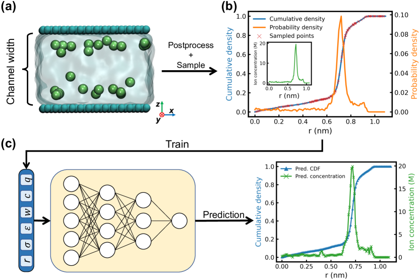
Figure 1: Framework of predicting ion profiles in nanochannels via NN. (a) Data is generated by running MD simulation of nanoconfined ionic solution. Channel width, $w$, is the surface-to-surface distance between the two charged graphene walls (colored teal). In the shown system, the ions are Na^+ (colored green) with molarity of 2 M and $w$ is 2 nm. (b) shows the probability and cumulative density of ion distribution in the nanochannel. $r$ is the distance from the $z$-direction center of the nanochannel. It is noticeable that the ion concentration distribution shown by the inset is just a linear transformation of the probability distribution. Data points are sampled from the cumulative density and used for the training of NN. (c) The NN model takes 6 inputs and predicts the cumulative density of ion within $r$ nm of the channel center. The predicted cumulative density is then translated to ion concentration profile.

II.1 Molecular dynamics simulation

The initial configurations of the ion-nanochannel systems are created using VMDHumphrey, Dalke, and Schulten (1996) and GROMACSBekker et al. (1993). Each system (Fig. 1a) contains a water box with ions sandwiched by two layers of graphene, which serve as the nanochannel walls. All systems have dimensions of 3.19 and 3.40 nm in the $x$ and $y$ direction, respectively. There are 832 carbon atoms in the simulation system. The surface-to-surface distance between the two graphene layers is the channel width denoted as $w$, ranging from 0.8 to 3.0 nm with the spacing of 0.1 nm ($w\in\{0.8,0.9,\cdots,3.0\}$, 23 variations). The number of water molecules in the nanochannel size of $3.19\times 3.40\times w$ is controlled such that the water density is at 1 g/cm^-3. Ions of different molarity, $c$, are added to the system, where $c$ ranges from 0.8 to 3.6 M changing by 0.2 M ($c\in\{0.8,1.0,\cdots,3.6\}$, 15 variations). Five types of ions are simulated including Na^+, Cl^-, K^+, Li^+, and Mg^2+. Each simulation system contains only one type of ion. To maintain charge neutrality, the same amount of opposite charges are evenly distributed to each carbon atom in the system, balancing the charge carried by the ions. In total, 1,725 simulations are run.

Table 1: The Lennard-Jones potentials and the charge of ions simulated in this work.

	NaJoung and Cheatham III (2008)	ClJoung and Cheatham III (2008)	MgCallahan et al. (2010)	LiJoung and Cheatham III (2008)	KJoung and Cheatham III (2008)	CBarati Farimani and Aluru (2011)
$\sigma$ ($\mathrm{\text{\r{A}}}$)	2.1600	4.8305	2.1200	1.4094	2.8384	3.3900
$\epsilon$ (kcal/mol)	0.3526	0.0128	0.8750	0.3367	0.4297	0.0692
$q$ (e)	+1	-1	+2	+1	+1	-

MD simulations are carried out using the LAMMPSPlimpton (1995) software. SPC/EMark and Nilsson (2001) water model is used to simulate water molecules. The interatomic potentials consist of the Lennard-Jones (LJ) potentials and long-range Coulombic interaction, both with a cutoff distance of 10 $\mathrm{\text{\r{A}}}$. The LJ potentials (Table 1) of ions and graphene are adopted from the ref Joung and Cheatham III (2008); Callahan et al. (2010); Chan and Hill (2010) and refBarati Farimani and Aluru (2011), respectively. Other interatomic potentials are calculated by the arithmetic rule. Nosé–Hoover thermostatNosé (1984); Hoover (1985) is used to maintain the temperature of the simulation system at 300 K. In each simulation, the system is firstly run under canonical (NVT) ensemble for 1 ns for the ions to reach equilibration positions. With the ensemble remains unchanged, the simulation is then run for another 1 ns while the trajectories are recorded every 5 ps. Periodic boundary condition is applied to all three dimensions. Post-processing of MD trajectories is conducted using the MDTrajMcGibbon et al. (2015) package.

II.2 Ion concentration profile as probability distribution

In this work, the ion concentration profile is regarded as the linear transformation of a conditional probability distribution (Fig. 1b). Namely, the ion concentration is the conditional probability multiplied with molar concentration. When the material of nanochannel wall and the solvent molecule remains unchanged (graphene and water in our case), the probability of the $z$-coordinate of a nanoconfined ion is at $r$ nm away from the channel center follows the conditional probability density function (PDF):

$$P(|z-o|=r\mid\sigma,\epsilon,w,c,q),$$ (1)

where $o$ is the $z$-coordinate of nanochannel center, $\sigma$ and $\epsilon$ are the LJ potentials of the ion, $w$ is the nanochannel width, $c$ is the molarity of ion in channel, and $q$ is the charge of the ion. If we denote the set including all conditions as $W=\{\sigma,\epsilon,w,c,q\}$, we get the conditional cumulative density function (CDF) as:

$$F(|z-o|=r\mid W)=P(|z-o|\leq r\mid W)=\frac{N_{|z-o|\leq r}}{N_{\mathrm{total}}},$$ (2)

where $N_{|z-o|\leq r}$ is the number of ions having $z$-coordinate within $r$ nm from the nanochannel center, and $N_{\mathrm{total}}$ is the total number of ions in the system. If the conditional CDF is known, then the ion concentration in any interval $r_{1}<|z-o|\leq r_{2}$ can be obtained simply by first calculating the conditional PDF:

$$P(r_{1}<|z-o|\leq r_{2}\mid W)=\\ F(|z-o|=r_{2}\mid W)-F(|z-o|=r_{1}\mid W)$$ (3)

and then multiplying it by the molar concentration.

Since acquiring true conditional CDF shown by Eq.2 is challenging, we propose to use a neural network parameterized by $\theta$, denoted as $F_{\theta}(\cdot)$, to approximate it:

$$F_{\theta}(|z-o|=r\mid W)\approx F(|z-o|=r\mid W).$$ (4)

Enough training data points should be sampled based on the true conditional CDF to ensure the expressivity of the neural networkGühring, Raslan, and Kutyniok (2020); Poole et al. (2016). In practice, we sample 2,000 data points using Eq.2 from each simulation (Fig. 1b). Among the 2,000 data points, half of them is sampled with uniformly chosen $r\in\{0,\frac{w}{2}+0.1\}$ nm, which ensures the model learns that no ion should be present outside of the nanochannel. The other half is sampled with uniformly chosen $r\in\{\mathrm{max}(0,\frac{w}{2}-0.5),\frac{w}{2}\}$ nm. Such a choice of interval includes more data points within 5 $\mathrm{\text{\r{A}}}$ of the nanochannel wall, thus helping the model to better learn the interfacial ion distribution. 3,450,000 data points are sampled in total from the 1,725 simulations. Each data point has features as $\{r,\sigma,\epsilon,w,c,q\}$ and labels as the conditional cumulative density $F(r\mid\sigma,\epsilon,w,c,q)$. Data points sampled from simulations with channel width $w\in\{1.6,2.4,2.8\}$ nm or with molarity $c\in\{1.4,2.2,3.0\}$ M are deposited into the test set, while the other ones into the training set. Overall, the training set contains 2,400,000 data points and the test set contains 1,050,000 data points.

II.3 Machine learning models and training

In our work, we use NN to model the conditional CDF, $F(|z-o|=r\mid W)$. Each sample $i$ in $N$ training data is denoted as $\{r_{i},W_{i},F_{i}\}$ representing the descriptor $W_{i}$ and its corresponding density function value $F_{i}$ at position $r_{i}$. The input to the machine learning models is thus a six-dimensional list $\{r_{i},W_{i}\}=\{r_{i},\sigma_{i},\epsilon_{i},w_{i},c_{i},q_{i}\}$, which describes the conditions and position to predict (Fig. 1). The output is $\tilde{F}_{i}$ which approximates the ground truth CDF $F_{i}$. An NN is developed as a surrogate model for ion concentration profile prediction. NN is based on fully-connected layers Rumelhart, Hinton, and Williams (1986); Hinton and Salakhutdinov (2006) and each layer is given:

$$y=a(W^{(l)}x),$$ (5)

where $x$ and $y$ are the input and output for each layer respectively, $W^{(l)}$ is the weight matrix at $l$-th layer, and $a$ is the element-wise nonlinear activation function. In our case, we used ReLUMaas et al. (2013) function for $a$ in all hidden layers and apply sigmoid in the output layer to guarantee the predicted cumulative density value is between 0 and 1. By stacking multiple fully-connected layers, NN can work as a universal function approximator LeCun, Bengio, and Hinton (2015) which is expected to accurately predict the conditional ion profiles. The objective of the NN is to minimize the MSE between the predictions $\{\tilde{F}_{i}\}_{i\in N}$ and the ground truth $\{{F}_{i}\}_{i\in N}$. The NN is implemented with five hidden layers and the number of units in each hidden layer is $\{1024,512,256,128,32\}$. We train the NN using Adam optimizer Kingma and Ba (2014) with a learning rate of 0.005 for 100 epochs.

To demonstrate the superior performance of NN, we benchmarked the prediction of ion profiles using another machine learning model, extreme gradient boosting (XGBoost). XGBoost is a gradient-boosted decision tree (GBDT) machine learning method and has demonstrated superior and robust performance in many applications Chen and Guestrin (2016). Unlike the NN, XGBoost is a non-parametric machine learning model without strong assumptions about the form of the mapping function from input to output. The model is based on decision trees which predict the labels via a series of if-then-else questions (levels) to the input features. An optimal decision tree estimates the minimum number of levels required to make a prediction during training. GBDT is an ensemble method for decision trees that combines multiple models to boost performance Mason et al. (1999); Ke et al. (2017). Specifically, GDBT leverages the error residual of the previous decision tree to train the next and ensembles all the decision trees by a weighted summation of the outputs of the models. For a GBDT $\tilde{F}_{M}$ with $M$ decision trees, the ensembled result is given:

$$\tilde{F}_{M}(z,W)=\sum_{m}^{M}\gamma_{m}T_{m}(r,W),$$ (6)

where $T_{m}$ denotes a single decision tree. And the weighted term $\gamma_{m}$ is calculated by:

$$\gamma_{m}=\operatorname*{arg\,min}_{\gamma}\sum_{i}^{N}\ell(F_{i},\tilde{F}_{m-1}(r_{i},W_{i})+\gamma T_{m}(r_{i},W_{i})),$$ (7)

where $\ell$ is a mean square error (MSE) loss $\ell(y,\tilde{y})=(y-\tilde{y})^{2}$ that measures the prediction accuracy. XGBoost is a scalable and distributed implementation of GDBT, which builds and trains decision trees in parallel. In our case, we set the level of decision trees as 15 and the $L_{2}$ regularization coefficient as 5 to mitigate overfitting. Other hyperparameters follow the default settings in the XGBoost packageChen and Guestrin (2016).

III Result and Discussion

III.1 Prediction of ion concentration profile

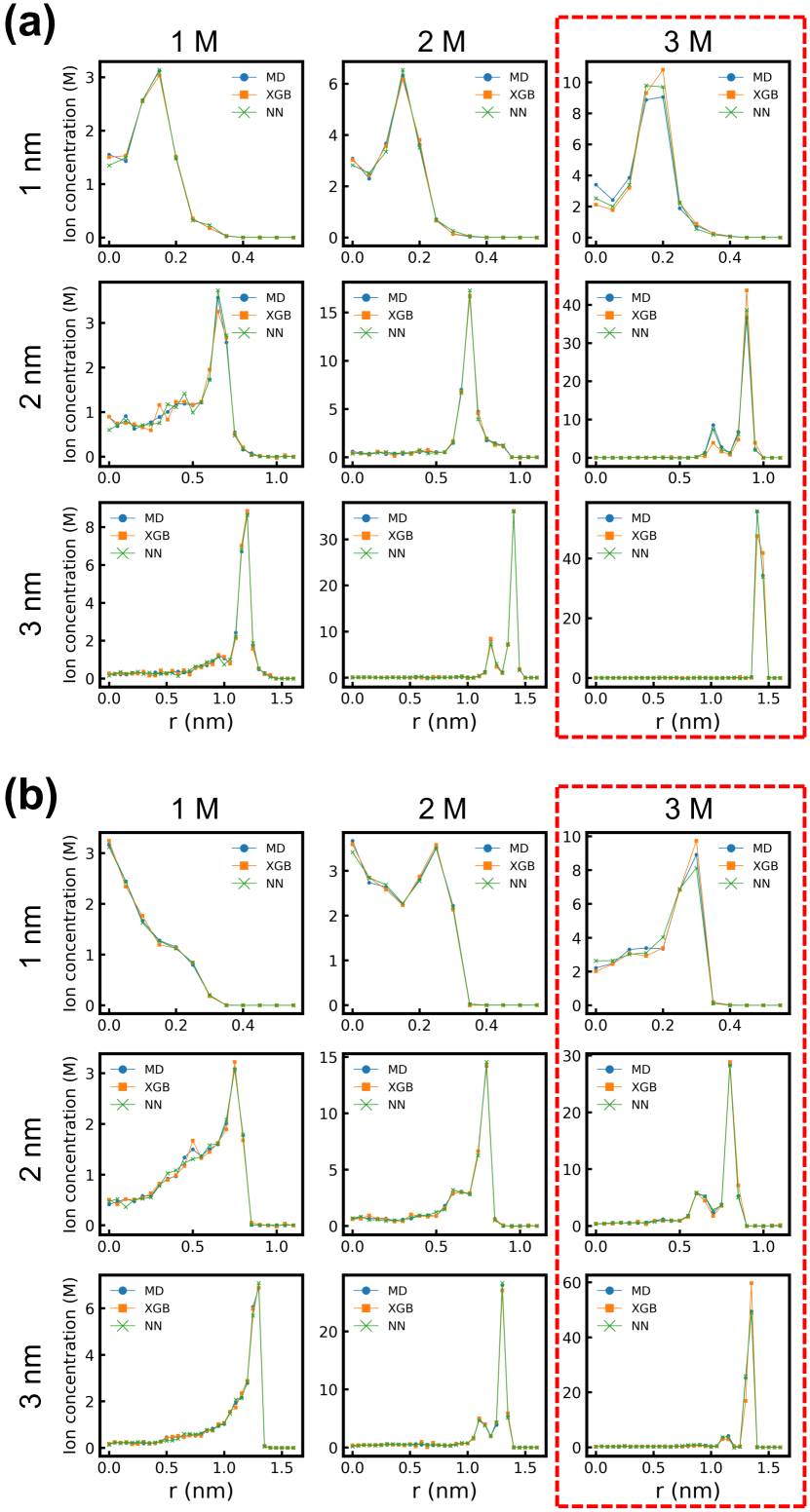
Figure 2: The comparison between ion concentration profiles predicted by MD simulation, neural network, and XGBoost model when channel width ranges from 1 to 3 nm and molarity ranges from 1 to 3 M. (a) shows the results of Na^+ and (b) shows the results of Cl^-. Results enclosed by the red dashed lines are included in the interpolation test set, while the others are included in the training set. $r$ represents the distance to the center of nanochannel.

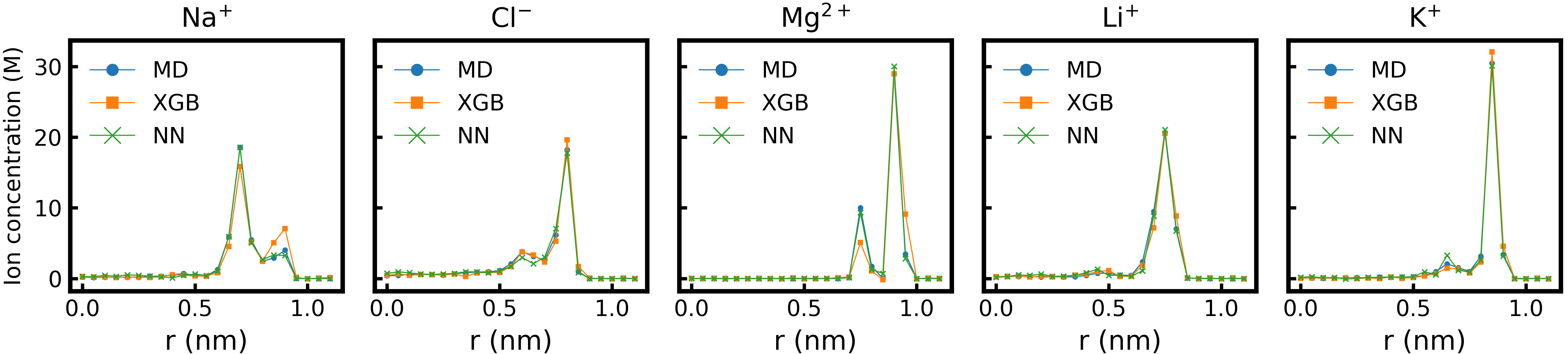
Figure 3: Comparison between model predicted ion concentration profile and MD simulation results for five different ions. The channel width is 2 nm and molarity is 2.2 M, which is a configuration included in the interpolation test set. Bin size is set as 0.05 nm.

To examine the performance of the NN and XGBoost models, we compare their predicted ion concentration profiles with the MD simulation results. Fig. 2 shows the ion concentration profile predicted using the three methods with different system configurations (combination of channel width and molarity), where the bin size is set as 0.05 nm. Plots enclosed by the red dashed lines have either channel width or molarity in the interpolation test set, while the other plots are results from the training set. For Na^+ (Fig. 2a), both models achieve close to perfect prediction for configurations in the training set. The location of the model-predicted concentration peaks fits perfectly with the MD simulation results. NN demonstrates more accurate interpolation capability than XGBoost as XGBoost has higher errors in predicting the peak concentration when molarity is 3 M. For Cl^- (Fig. 2b), XGBoost shows a tendency of overpredicting the peak concentration when the molarity is at 3 M. A single layer of Cl^- occurs in the configuration [1 nm, 1 M], which is different from the other configurations where ion concentration peak occurs closer to the nanoconfinement wall. Both models accurately capture such a physical phenomenon. One small error made by NN is that it fails to predict the secondary concentration peak located at 0.5 nm from the channel center in the configuration [2 nm, 1 M]. In general, Fig. 2 demonstrates that NN is capable of accurately predicting the ion concentration profile by learning the CDF of ion in nanochannel, and NN interpolates better on unseen configurations compared with XGBoost.

Another variable besides channel width and molarity is the ion type. Fig. 3 shows the comparison between model-predicted ion concentration profiles and MD simulation results for five different ions. The channel width is 2 nm, the molarity is 2.2 M, and the bin size is 0.05 nm for all subplots in Fig. 3. It can be observed that the location of peaks predicted by both NN and XGBoost is correct compared with MD results. For Na^+, XGBoost underpredicts the concentration of the primary peak while largely overpredicting the secondary peak. XGBoost also significantly underpredicts the concentration of the secondary peak of Mg^2+. Despite minor prediction error found on the secondary peaks of Cl^- and K^+ profiles, NN is shown to be a more accurate model than XGBoost in this task. Ion concentration profiles of all configurations are available on the GitHub page of this work. Fig. 3 shows that NN bears the potential as a generalizable predictor of ion concentration profile regardless of the type and charge of the ions.

III.2 Error analysis and inference time

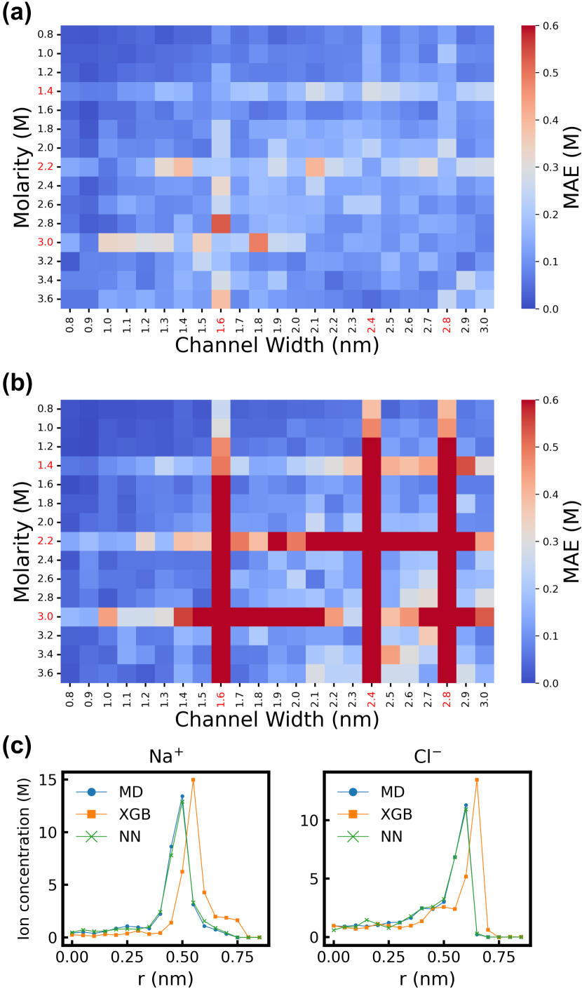
Figure 4: Mean absolute error of (a) NN and (b) XGBoost predicted Na^+ concentration profile in all system configurations. MAE is calculated based on the profiles with bin size of 0.05 nm. The highest MAE of XGBoost in the dark red blocks is 4.92 M. The maximum value of the color bar is truncated such that the MAE of NN can be distinguished. The tick labels of channel width and molarity in the test set are colored red. (c) shows examples of failed interpolation of XGBoost for the configuration [1.6 nm, 2.2 M] due to overfitting.

To thoroughly evaluate NN and XGBoost as a surrogate model to MD simulation, we benchmarked both models on their prediction accuracy and inference time. The mean absolute error (MAE) of Na^+ concentration profile prediction is the first metric of accuracy. Fig. 4a and 4b visualize the MAE heatmap of NN and XGBoost, respectively, for all simulated configurations. The MAE is calculated based on concentration profiles with bin size of 0.05 nm. The tick labels of the channel width and molarity included in the interpolation test set are colored red. Despite a slight increase of MAE when interpolating, NN achieves high prediction accuracy for all configurations. The highest MAE of NN is 0.53 M in the configuration [1.6 nm, 2.8 M]. On the other hand, the prediction accuracy of XGBoost suffers from overfitting. When interpolating Na^+ concentration profile for 1.6, 2.4, 3.0 nm channel width and 1.4, 2.2, 3.0 M molarity, MAE of XGBoost drastically increases. The highest MAE of XGBoost is 4.92 M, which occurs in the configuration [1.6 nm, 3.6 M]. The maximum value of the color bar of the heatmap is truncated at 0.6 M so that low MAE is more visible. Examples of XGBoost overfitting Na^+ and Cl^- concentration profiles in configuration [1.6 nm, 2 M] are shown in Fig. 4c. For both Na^+ and Cl^-, the concentration peaks are mispredicted by XGBoost to be 0.05 nm away from the MD simulation results, leading to exceptionally high MAE. On the other hand, overfitting has a trivial effect on the prediction accuracy of NN. When channel width is 2.4 nm, no obvious MAE increase is shown in Fig. 4a.

Table 2: Evaluation of the interpolation error and inference time of NN and XGBoost. All metrics are calculated given the bin size of 0.05 nm. Both MAE and peak deviation are averaged over all configurations in the interpolation set. Inference time measures the total time to generate ion concentration profiles for all 1,725 configurations (5 ions, 23 channel width, 15 molarity). The inference time of MD does not include the time used to load molecular trajectories. The inference time reported is averaged over 6 runs, with the standard deviation in parentheses. The lower value of each metric is the better model.

	NN	XGBoost	MD
Interp. MAE (M)	0.1899	1.2764	-
Interp. peak deviation (nm)	0.0019	0.0314	-
Inference time (s)	0.80(0.10)	2.56(0.11)	11.72(0.42)

Two metrics, MAE and peak deviation are calculated to quantitatively evaluate the advantage of NN in interpolation (Table 2). MAE measures the prediction error of the whole ion concentration profile. Peak deviation measures how well the shape of the predicted ion concentration profile is aligned with the MD simulation result. The lower the value for each metric, the better the model is expected in interpolation. The interpolation MAE of NN is only 14.9% of that of XGBoost. Moreover, the interpolation peak deviation of NN is 0.0019 nm, which is only 6.1% of that of XGBoost. Both metrics prove that NN does not suffer from overfitting as XGBoost does, and is capable of accurately interpolating ion concentration profiles under different nanoconfinement conditions.

Using machine learning as a fast surrogate model for MD simulation is the major motivation for this work. To evaluate the improvement in computation speed, we benchmark the inference time of NN, XGBoost, and MD simulation. Here, we define the inference time to be the total time taken to predict the ion concentration profiles of all 1,725 system configurations (5 ions, 23 channel widths, 15 molarities) with bin size as 0.05 nm. For MD simulation, we only consider the postprocessing time of the molecular trajectories using MDTrajMcGibbon et al. (2015) and NumPyHarris et al. (2020); Van Der Walt, Colbert, and Varoquaux (2011). The time of loading molecular trajectories is not included for a fair comparison. The benchmark is conducted with an Intel Core i7-8086K CPU for all models (Table 2). Averaged over 6 runs, NN can predict all 1,725 ion concentration profiles in 0.8 s, whereas XGBoost takes 2.56 s and processing MD trajectories takes 11.72 s. NN is approximately 3.2$\times$ faster than XGBoost and 14.7$\times$ faster than processing MD simulation trajectories. The inference time benchmark demonstrates that NN is a fast surrogate model for MD simulation. It is noteworthy that running a single MD simulation takes about 8 hours on average using 6 CPU cores, indicating that running all 1,725 simulations takes approximately 82,800 core-hours. If we compare the inference time of NN to the time required to run MD simulation, NN is orders of magnitude faster. Considering the size of NN model is 2.8 MB, which is much smaller than XGBoost model (71.1 MB) and MD simulation trajectories (32.1 GB), NN is also more storage-efficient than the other two.

III.3 Sampling with different bin sizes

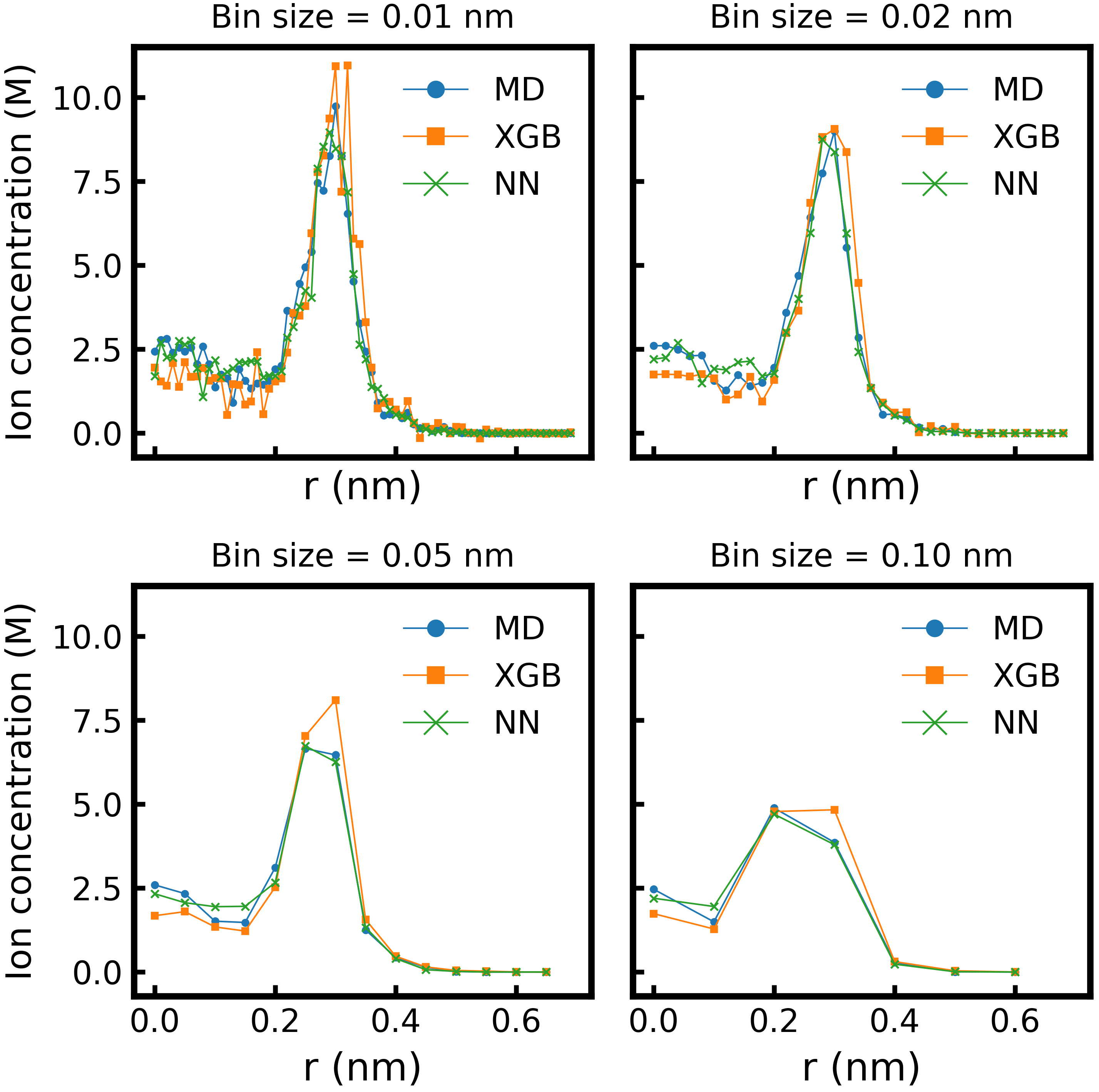
Figure 5: Predicted Na^+ concentration profile with bin size ranging from 0.01 to 0.1 nm. The shown configuration is [1.2 nm, 2.2 M], which is included in the interpolation set.

One advantage of training a NN to learn the CDF instead of the whole ion concentration profile is the flexibility of sampling. By sampling on the CDF and converting probability to ion concentration, the NN can predict ion concentration profiles with arbitrary bin sizes. Fig. 5 shows the prediction of Na^+ concentration profile in the configuration [1.2 nm, 2.2 M] with bin size ranging from 0.01 to 0.1 nm. Both NN and XGBoost successfully model the shape of the profile regardless of the bin size: a primary peak near the confinement wall and a secondary peak at the channel center. When bin size is as fine as 0.01 nm, the concentration profile near the channel center is noisy because of less ion presence. Given the stochastic nature of MD simulation, which is used to generate the training data, the minor prediction error near the channel center with such a fine bin size is expected. The effect of stochasticity reduces as the bin size increases, resulting in more accurate predictions by NN and XGBoost.

IV Conclusion

In this work, we show the viability of using a neural network (NN) as a surrogate model for MD simulation in predicting the ion concentration profile in the nanochannel. We first model the ion concentration profile in nanochannel as a probability distribution conditioned on the configuration of nanochannel systems, such as LJ potentials of the ion, channel width, and molarity of ion. A NN is then trained to predict the conditional cumulative density probability (CDF) distribution of ions given the system configuration. The predicted CDF can be linearly transformed back to the concentration profile as the final output of the NN model. 1,725 MD simulations (5 types of ions, 23 variations of channel width, 15 variations of molarity) are run to generate training and test data for the NN model.

We benchmark NN against another machine learning model, XGBoost, to compare their interpolation ability. The two metrics we used are the mean absolute error (MAE) of the whole interpolated ion concentration profile, and the peak deviation from the MD simulation concentration profile. On average, NN achieves 85.1% lower mean absolute error and 93.9% lower peak deviation when interpolating Na^+ concentration profiles compared with the XGBoost model. Such a benchmark demonstrates the superior ability of NN to interpolate ion concentration profiles given unseen system configurations. Further, we record the inference time taken by the NN and XGBoost models and compared that to the time taken to post-process MD simulation trajectories. To predict 1,725 ion concentration profiles, NN takes an inference time of 0.80 s, which is approximately 3.2$\times$ and 14.7$\times$ faster than the XGBoost and processing MD trajectories, respectively. At last, we show that NN can flexibly predict ion concentration profile with any bin size. The accuracy of NN prediction increases with larger bin sizes because of the reduced effect of stochasticity. In conclusion, NN is a fast, flexible, and most importantly, accurate surrogate model to predict ion concentration profiles under nanoconfinement.

Data Availability Statement

The training data used for machine learning model training are openly available on GitHub (https://github.com/zcao0420/IonNet).

References

- Sun et al. (2020) C. Sun, R. Zhou, Z. Zhao, and B. Bai, “Nanoconfined fluids: What can we expect from them?” The Journal of Physical Chemistry Letters 11, 4678–4692 (2020).
- Thomas and McGaughey (2008) J. A. Thomas and A. J. McGaughey, “Reassessing fast water transport through carbon nanotubes,” Nano letters 8, 2788–2793 (2008).
- Wu et al. (2017) K. Wu, Z. Chen, J. Li, X. Li, J. Xu, and X. Dong, “Wettability effect on nanoconfined water flow,” Proceedings of the National Academy of Sciences 114, 3358–3363 (2017).
- Barati Farimani and Aluru (2011) A. Barati Farimani and N. R. Aluru, “Spatial diffusion of water in carbon nanotubes: from fickian to ballistic motion,” The Journal of Physical Chemistry B 115, 12145–12149 (2011).
- Wang and Hadjiconstantinou (2018) G. J. Wang and N. G. Hadjiconstantinou, “Layered fluid structure and anomalous diffusion under nanoconfinement,” Langmuir 34, 6976–6982 (2018).
- Cao and Farimani (2022) Z. Cao and A. B. Farimani, “The diffusion mechanism of water in conductive metal–organic frameworks,” Physical Chemistry Chemical Physics 24, 24852–24859 (2022).
- Barati Farimani and Aluru (2016) A. Barati Farimani and N. R. Aluru, “Existence of multiple phases of water at nanotube interfaces,” The Journal of Physical Chemistry C 120, 23763–23771 (2016).
- Giovambattista, Rossky, and Debenedetti (2009) N. Giovambattista, P. J. Rossky, and P. G. Debenedetti, “Phase transitions induced by nanoconfinement in liquid water,” Physical review letters 102, 050603 (2009).
- Mondal and Bagchi (2020) S. Mondal and B. Bagchi, “How different are the dynamics of nanoconfined water?” The Journal of Chemical Physics 152, 224707 (2020).
- Hu et al. (2010) M. Hu, J. V. Goicochea, B. Michel, and D. Poulikakos, “Water nanoconfinement induced thermal enhancement at hydrophilic quartz interfaces,” Nano letters 10, 279–285 (2010).
- Pan et al. (2020) J. Pan, S. Xiao, Z. Zhang, N. Wei, J. He, and J. Zhao, “Nanoconfined water dynamics in multilayer graphene nanopores,” The Journal of Physical Chemistry C 124, 17819–17828 (2020).
- Rojano et al. (2022) A. Rojano, A. Córdoba, J. H. Walther, and H. A. Zambrano, “Effect of charge inversion on nanoconfined flow of multivalent ionic solutions,” Physical Chemistry Chemical Physics 24, 4935–4943 (2022).
- Qiu, Ma, and Chen (2016) Y. Qiu, J. Ma, and Y. Chen, “Ionic behavior in highly concentrated aqueous solutions nanoconfined between discretely charged silicon surfaces,” Langmuir 32, 4806–4814 (2016).
- Tan et al. (2022) J. Tan, Z. Li, M. Ye, and J. Shen, “Nanoconfined space: Revisiting the charge storage mechanism of electric double layer capacitors,” ACS Applied Materials & Interfaces 14, 37259–37269 (2022).
- Qiao and Aluru (2004) R. Qiao and N. R. Aluru, “Charge inversion and flow reversal in a nanochannel electro-osmotic flow,” Physical review letters 92, 198301 (2004).
- Alizadeh et al. (2021) A. Alizadeh, W.-L. Hsu, M. Wang, and H. Daiguji, “Electroosmotic flow: From microfluidics to nanofluidics,” Electrophoresis 42, 834–868 (2021).
- Qian, Gao, and Pan (2020) J. Qian, X. Gao, and B. Pan, “Nanoconfinement-mediated water treatment: from fundamental to application,” Environmental Science & Technology 54, 8509–8526 (2020).
- Cao, Liu, and Barati Farimani (2019) Z. Cao, V. Liu, and A. Barati Farimani, “Water desalination with two-dimensional metal–organic framework membranes,” Nano letters 19, 8638–8643 (2019).
- Wang, Cao, and Barati Farimani (2021) Y. Wang, Z. Cao, and A. Barati Farimani, “Efficient water desalination with graphene nanopores obtained using artificial intelligence,” npj 2D Materials and Applications 5, 66 (2021).
- Mei et al. (2022) L. Mei, Z. Cao, T. Ying, R. Yang, H. Peng, G. Wang, L. Zheng, Y. Chen, C. Y. Tang, D. Voiry, et al., “Simultaneous electrochemical exfoliation and covalent functionalization of mos2 membrane for ion sieving,” Advanced Materials 34, 2201416 (2022).
- Cao, Liu, and Barati Farimani (2020) Z. Cao, V. Liu, and A. Barati Farimani, “Why is single-layer mos2 a more energy efficient membrane for water desalination?” ACS Energy Letters 5, 2217–2222 (2020).
- Cao, Markey, and Barati Farimani (2021) Z. Cao, G. Markey, and A. Barati Farimani, “Ozark graphene nanopore for efficient water desalination,” The Journal of Physical Chemistry B 125, 11256–11263 (2021).
- Zhu et al. (2019) H. Zhu, Y. Wang, Y. Fan, J. Xu, and C. Yang, “Structure and transport properties of water and hydrated ions in nano-confined channels,” Advanced Theory and Simulations 2, 1900016 (2019).
- Kong et al. (2017) J. Kong, Z. Bo, H. Yang, J. Yang, X. Shuai, J. Yan, and K. Cen, “Temperature dependence of ion diffusion coefficients in nacl electrolyte confined within graphene nanochannels,” Physical Chemistry Chemical Physics 19, 7678–7688 (2017).
- Freund (2002) J. B. Freund, “Electro-osmosis in a nanometer-scale channel studied by atomistic simulation,” The Journal of Chemical Physics 116, 2194–2200 (2002).
- Kékicheff et al. (1993) P. Kékicheff, S. Marcelja, T. Senden, and V. Shubin, “Charge reversal seen in electrical double layer interaction of surfaces immersed in 2: 1 calcium electrolyte,” The Journal of chemical physics 99, 6098–6113 (1993).
- Sendner et al. (2009) C. Sendner, D. Horinek, L. Bocquet, and R. R. Netz, “Interfacial water at hydrophobic and hydrophilic surfaces: Slip, viscosity, and diffusion,” Langmuir 25, 10768–10781 (2009).
- Qiao and Aluru (2003a) R. Qiao and N. Aluru, “Atypical dependence of electroosmotic transport on surface charge in a single-wall carbon nanotube,” Nano letters 3, 1013–1017 (2003a).
- Robin et al. (2023) P. Robin, A. Delahais, L. Bocquet, and N. Kavokine, “Ion filling of a one-dimensional nanofluidic channel in the interaction confinement regime,” arXiv preprint arXiv:2301.04622 (2023).
- Meidani, Cao, and Barati Farimani (2021) K. Meidani, Z. Cao, and A. Barati Farimani, “Titanium carbide mxene for water desalination: a molecular dynamics study,” ACS Applied Nano Materials 4, 6145–6151 (2021).
- Qiao and Aluru (2003b) R. Qiao and N. R. Aluru, “Ion concentrations and velocity profiles in nanochannel electroosmotic flows,” The Journal of chemical physics 118, 4692–4701 (2003b).
- Zhou and Xu (2020) K. Zhou and Z. Xu, “Field-enhanced selectivity in nanoconfined ionic transport,” Nanoscale 12, 6512–6521 (2020).
- Brunton, Noack, and Koumoutsakos (2020) S. L. Brunton, B. R. Noack, and P. Koumoutsakos, “Machine learning for fluid mechanics,” Annual review of fluid mechanics 52, 477–508 (2020).
- Brunton, Proctor, and Kutz (2016) S. L. Brunton, J. L. Proctor, and J. N. Kutz, “Discovering governing equations from data by sparse identification of nonlinear dynamical systems,” Proceedings of the national academy of sciences 113, 3932–3937 (2016).
- Cranmer et al. (2020) M. Cranmer, A. Sanchez Gonzalez, P. Battaglia, R. Xu, K. Cranmer, D. Spergel, and S. Ho, “Discovering symbolic models from deep learning with inductive biases,” Advances in Neural Information Processing Systems 33, 17429–17442 (2020).
- Meidani and Farimani (2023) K. Meidani and A. B. Farimani, “Identification of parametric dynamical systems using integer programming,” Expert Systems with Applications , 119622 (2023).
- Davies et al. (2021) A. Davies, P. Veličković, L. Buesing, S. Blackwell, D. Zheng, N. Tomašev, R. Tanburn, P. Battaglia, C. Blundell, A. Juhász, et al., “Advancing mathematics by guiding human intuition with ai,” Nature 600, 70–74 (2021).
- Li et al. (2022) Z. Li, K. Meidani, P. Yadav, and A. Barati Farimani, “Graph neural networks accelerated molecular dynamics,” The Journal of Chemical Physics 156, 144103 (2022).
- Moradzadeh, Oliaei, and Aluru (0) A. Moradzadeh, H. Oliaei, and N. R. Aluru, “Topology-based phase identification of bulk, interface, and confined water using an edge-conditioned convolutional graph neural network,” The Journal of Physical Chemistry C 0, null (0), https://doi.org/10.1021/acs.jpcc.2c07423 .
- Wu and Aluru (2022) H. Wu and N. Aluru, “Deep learning-based quasi-continuum theory for structure of confined fluids,” The Journal of Chemical Physics 157, 084121 (2022).
- Santos et al. (2020) J. E. Santos, M. Mehana, H. Wu, M. Prodanovic, Q. Kang, N. Lubbers, H. Viswanathan, and M. J. Pyrcz, “Modeling nanoconfinement effects using active learning,” The Journal of Physical Chemistry C 124, 22200–22211 (2020).
- Lubbers et al. (2020) N. Lubbers, A. Agarwal, Y. Chen, S. Son, M. Mehana, Q. Kang, S. Karra, C. Junghans, T. C. Germann, and H. S. Viswanathan, “Modeling and scale-bridging using machine learning: nanoconfinement effects in porous media,” Scientific Reports 10, 13312 (2020).
- Leverant et al. (2021) C. J. Leverant, J. A. Harvey, T. M. Alam, and J. A. Greathouse, “Machine learning self-diffusion prediction for lennard-jones fluids in pores,” The Journal of Physical Chemistry C 125, 25898–25906 (2021).
- Hanin (2019) B. Hanin, “Universal function approximation by deep neural nets with bounded width and relu activations,” Mathematics 7, 992 (2019).
- Scarselli and Tsoi (1998) F. Scarselli and A. C. Tsoi, “Universal approximation using feedforward neural networks: A survey of some existing methods, and some new results,” Neural networks 11, 15–37 (1998).
- Lu and Lu (2020) Y. Lu and J. Lu, “A universal approximation theorem of deep neural networks for expressing probability distributions,” Advances in neural information processing systems 33, 3094–3105 (2020).
- Magdon-Ismail and Atiya (1998) M. Magdon-Ismail and A. Atiya, “Neural networks for density estimation,” Advances in Neural Information Processing Systems 11 (1998).
- Liu et al. (2021) Q. Liu, J. Xu, R. Jiang, and W. H. Wong, “Density estimation using deep generative neural networks,” Proceedings of the National Academy of Sciences 118, e2101344118 (2021).
- Rothfuss et al. (2019) J. Rothfuss, F. Ferreira, S. Walther, and M. Ulrich, “Conditional density estimation with neural networks: Best practices and benchmarks,” arXiv preprint arXiv:1903.00954 (2019).
- Humphrey, Dalke, and Schulten (1996) W. Humphrey, A. Dalke, and K. Schulten, “Vmd: visual molecular dynamics,” Journal of molecular graphics 14, 33–38 (1996).
- Bekker et al. (1993) H. Bekker, H. Berendsen, E. Dijkstra, S. Achterop, R. Vondrumen, D. Vanderspoel, A. Sijbers, H. Keegstra, and M. Renardus, “Gromacs-a parallel computer for molecular-dynamics simulations,” in 4th international conference on computational physics (PC 92) (World Scientific Publishing, 1993) pp. 252–256.
- Joung and Cheatham III (2008) I. S. Joung and T. E. Cheatham III, “Determination of alkali and halide monovalent ion parameters for use in explicitly solvated biomolecular simulations,” The journal of physical chemistry B 112, 9020–9041 (2008).
- Callahan et al. (2010) K. M. Callahan, N. N. Casillas-Ituarte, M. Roeselová, H. C. Allen, and D. J. Tobias, “Solvation of magnesium dication: molecular dynamics simulation and vibrational spectroscopic study of magnesium chloride in aqueous solutions,” The Journal of Physical Chemistry A 114, 5141–5148 (2010).
- Plimpton (1995) S. Plimpton, “Fast parallel algorithms for short-range molecular dynamics,” Journal of computational physics 117, 1–19 (1995).
- Mark and Nilsson (2001) P. Mark and L. Nilsson, “Structure and dynamics of the tip3p, spc, and spc/e water models at 298 k,” The Journal of Physical Chemistry A 105, 9954–9960 (2001).
- Chan and Hill (2010) Y. Chan and J. Hill, “Modelling interaction of atoms and ions with graphene,” Micro & Nano Letters 5, 247–250 (2010).
- Nosé (1984) S. Nosé, “A Unified Formulation of the Constant Temperature Molecular Dynamics Methods,” J. Chem. Phys. 81, 511–519 (1984).
- Hoover (1985) W. G. Hoover, “Canonical Dynamics: Equilibrium Phase-Space Distributions,” Phys. Rev. A 31, 1695 (1985).
- McGibbon et al. (2015) R. T. McGibbon, K. A. Beauchamp, M. P. Harrigan, C. Klein, J. M. Swails, C. X. Hernández, C. R. Schwantes, L.-P. Wang, T. J. Lane, and V. S. Pande, “Mdtraj: A modern open library for the analysis of molecular dynamics trajectories,” Biophysical Journal 109, 1528 – 1532 (2015).
- Gühring, Raslan, and Kutyniok (2020) I. Gühring, M. Raslan, and G. Kutyniok, “Expressivity of deep neural networks,” arXiv preprint arXiv:2007.04759 (2020).
- Poole et al. (2016) B. Poole, S. Lahiri, M. Raghu, J. Sohl-Dickstein, and S. Ganguli, “Exponential expressivity in deep neural networks through transient chaos,” Advances in neural information processing systems 29 (2016).
- Rumelhart, Hinton, and Williams (1986) D. E. Rumelhart, G. E. Hinton, and R. J. Williams, “Learning representations by back-propagating errors,” nature 323, 533–536 (1986).
- Hinton and Salakhutdinov (2006) G. E. Hinton and R. R. Salakhutdinov, “Reducing the dimensionality of data with neural networks,” science 313, 504–507 (2006).
- Maas et al. (2013) A. L. Maas, A. Y. Hannun, A. Y. Ng, et al., “Rectifier nonlinearities improve neural network acoustic models,” in Proc. icml, Vol. 30 (Atlanta, Georgia, USA, 2013) p. 3.
- LeCun, Bengio, and Hinton (2015) Y. LeCun, Y. Bengio, and G. Hinton, “Deep learning,” nature 521, 436–444 (2015).
- Kingma and Ba (2014) D. P. Kingma and J. Ba, “Adam: A method for stochastic optimization,” arXiv preprint arXiv:1412.6980 (2014).
- Chen and Guestrin (2016) T. Chen and C. Guestrin, “Xgboost: A scalable tree boosting system,” in Proceedings of the 22nd acm sigkdd international conference on knowledge discovery and data mining (2016) pp. 785–794.
- Mason et al. (1999) L. Mason, J. Baxter, P. Bartlett, and M. Frean, “Boosting algorithms as gradient descent,” Advances in neural information processing systems 12 (1999).
- Ke et al. (2017) G. Ke, Q. Meng, T. Finley, T. Wang, W. Chen, W. Ma, Q. Ye, and T.-Y. Liu, “Lightgbm: A highly efficient gradient boosting decision tree,” Advances in neural information processing systems 30 (2017).
- Harris et al. (2020) C. R. Harris, K. J. Millman, S. J. Van Der Walt, R. Gommers, P. Virtanen, D. Cournapeau, E. Wieser, J. Taylor, S. Berg, N. J. Smith, et al., “Array programming with numpy,” Nature 585, 357–362 (2020).
- Van Der Walt, Colbert, and Varoquaux (2011) S. Van Der Walt, S. C. Colbert, and G. Varoquaux, “The numpy array: a structure for efficient numerical computation,” Computing in science & engineering 13, 22–30 (2011).