An Experimental Study of Two-Level Schwarz Domain Decomposition Preconditioners on GPUs

Abstract

The generalized Dryja–Smith–Widlund (GDSW) preconditioner is a two-level overlapping Schwarz domain decomposition (DD) preconditioner that couples a classical one-level overlapping Schwarz preconditioner with an energy-minimizing coarse space. When used to accelerate the convergence rate of Krylov subspace iterative methods, the GDSW preconditioner provides robustness and scalability for the solution of sparse linear systems arising from the discretization of a wide range of partial different equations. In this paper, we present FROSch (Fast and Robust Schwarz), a domain decomposition solver package which implements GDSW-type preconditioners for both CPU and GPU clusters. To improve the solver performance on GPUs, we use a novel decomposition to run multiple MPI processes on each GPU, reducing both solver’s computational and storage costs and potentially improving the convergence rate. This allowed us to obtain competitive or faster performance using GPUs compared to using CPUs alone. We demonstrate the performance of FROSch on the Summit supercomputer with NVIDIA V100 GPUs, where we used NVIDIA Multi-Process Service (MPS) to implement our decomposition strategy.

The solver has a wide variety of algorithmic and implementation choices, which poses both opportunities and challenges for its GPU implementation. We conduct a thorough experimental study with different solver options including the exact or inexact solution of the local overlapping subdomain problems on a GPU. We also discuss the effect of using the iterative variant of the incomplete LU factorization and sparse-triangular solve as the approximate local solver, and using lower precision for computing the whole FROSch preconditioner. Overall, the solve time was reduced by factors of about $2\times$ using GPUs, while the GPU acceleration of the numerical setup time depend on the solver options and the local matrix sizes.

I Introduction

Domain decomposition methods (DDMs) [26, 13] may be used to build a class of effective parallel solvers for sparse linear systems arising from the discretization of partial differential equations. In DDMs, the global problem is decomposed into smaller local subproblems, which can be processed in parallel. As a result, DDM preconditioners are well-suited for solving large-scale linear systems on distributed-memory computers. However, for one-level DDMs, the number of iterations required for the solution convergence typically increases with an increasing number of subdomains. As a remedy, a second-level coarse system, which is determined by carefully-designed coarse basis functions, is introduced. As a results the condition number of the preconditioned matrix, and thus the required number of iterations, becomes asymptotically independent of the number of subdomains. In this paper, we consider the generalized Dryja–Smith–Widlund (GDSW) [11] two-level Schwarz DDM, which combines classical one-level overlapping additive Schwarz preconditioner with energy-minimizing coarse basis functions and has been shown to be robust and scalable for solving many challenging problems.

Our focus is on the GPU performance of the GDSW preconditioner. Several algorithmic and software options are possible for the GDSW algorithm. Each of these options has multiple tunable parameters, and a good choice of the parameters can be architecture and problem specific. Some of these options also have algorithmic implications in addition to the implementation choices. For example, the computational complexity of the local sparse solver increases more than linearly to the local matrix size. Since there are typically more CPU cores than the GPUs, decomposing the global domain to one subdomain per GPU instead of one subdomain per CPU core may increase the complexity of the local subdomain solver. Moreover, a fewer subdomains lead to a smaller coarse space, which could degrade the convergence behavior. Finally, many of the kernels, which DDM solvers depend on, such as sparse direct solver, incomplete factorization, sparse triangular solver, and sparse matrix-matrix multiply, are difficult to optimize on GPUs. All of these properties pose challenges when implementing the solver and tuning its performance for the GPU architectures. As a result, the comprehensive GPU performance study of two-level DDM solver has been lacking, especially at scale, to the best of our knowledge.

	used	effects	other options available
Krylov solver	single-reduce GMRES	improve data access	standard, pipelined, comm-avoid
GDSW	two-level rGDSW	reduce coarse space size	standard, multi-level
Direct solver	GPU-enabled Tacho	allows use of GPU	CPU-only, e.g., SuperLU
Sparse triangular solve	supernode-based Kokkos-Kernels	improve GPU utilization	element-based, partitioned inverse
Inexact solver	iterative variants FastILU/FastSpTRSV	expose more parallelism	standard on CPU/GPU
Precision	single precision HalfPrecisionOp	reduce data volume	uniform double precision
# of subdomains	# of CPU cores	reduce solver costs	# of GPUs
		& improve convergence

TABLE I: Solver options used in this paper: each solver option has multiple tunable parameters, e.g., GMRES with restart length, orthogonalization scheme, rGDSW with size of overlap, Tacho with matrix ordering scheme, FastILU with number of levels, and Jacobi iteration count and damping factor, just to name a few main parameters.

To fill this gap, we study the GPU performance of FROSch (Fast and Robust Schwarz), a solver package, which implements GDSW preconditioners within Trilinos software framework; cf. [18]. Our implementation is also portable to different hardware architectures with a single code base. As architectures change rapidly, it is critical to design the software stack such that the solver is portable to different hardware architectures (e.g., isolating the hardware-specific codes and optimizations from the high-level solver design and implementation). Though this avoids the need of re-writing the solver for each new architecture, in order to obtain high performance on a specific architecture, including on a GPU cluster, the software stack must be carefully designed and new variants of the algorithms may be needed. We evaluate many of the algorithmic and software choices that are critical for the GPU performance of the GDSW preconditioners including new solver capabilities added for this purpose, e.g.,

• single-reduce variant [30] of the Krylov solver, which performs only one global-reduce for each iteration,

• the exact solution of the local overlapping subdomain and coarse space problems based on the direct sparse LU factorization on a GPU [21],

• a supernodal-based sparse triangular solver [28], which reduces the number of kernel launches and exploit the hierarchical parallelism available on a GPU, and

• iterative variants of ILU factorization and sparse-triangular solver [8], which have much higher costs of computation but expose more parallelism than the standard substitution-based algorithm.

Table I lists some of the main solver options, which we will evaluate in this paper, and other parameters we selected based on our experience and past results.

Experimental results on the Summit supercomputer with NVIDIA V100 GPUs demonstrate the potential of the two-level DD solvers on the GPU clusters. We compare the GPU performance with the CPU performance using all the CPU cores on each node. We believe this provides a conservative but fair performance comparison that an application is expected to see. Using GPUs, the solve time for 3D elasticity problems was reduced by factors of around $2\times$, while the effects on the numerical solver setup time depends on the solver options and the local matrix sizes. In cases of using local direct solvers, the total solution time (the total of the numerical setup and solve time) for a single linear system was reduced by a factor of about $1.1\times$ to $1.7\times$. If the application requires to solve a sequence of the linear systems with different right-hand-sides, the cost of the numerical setup can be amortized over multiple solves and the speedups closer to $2\times$ can be obtained.

The main contributions of this work are:

• A GPU implementation and large-scale GPU performance study of a two-level DDM solver;

• A novel decomposition strategy that allows the use of NVIDIA Multi-Process Service (MPS) to run multiple MPI processes on each GPU, and significantly reduces both the computational and storage cost of the DDM solver, and potentially improves convergence (Section VI). We are not aware of other studies, which use MPS with a production-ready linear solver. In our performance studies of using MPS on Summit, both the numerical setup and solve time of FROSch was reduced by the factors of up to $3\times$.

• A detailed experimental study of several solver options for the two-level DDM including direct, incomplete, and approximate factorizations, with multiple parameter choices for each of them.

• Numerical and GPU performance studies with inexact or approximate local linear solver or with DDM preconditioner in a lower precision, enabling the solution of larger-scale linear systems than the linear system that the typical DDM solvers can (the exact solution with local direct solvers in double precision, which typical GDSW in practice, and its theory, is based on).

II Related Work

As GPUs became a critical part in scientific computing, there have been several works to optimize the computational kernels, which are also needed for DDM solvers. On the other hand, a GPU implementation of a two-level DDM solver that uses these kernels in addition to other kernels has not been demonstrated at scale. Luo et al. [22] investigated the GPU performance of a one-level DDM, and the number of MPI processes was limited by the number of GPUs. We will show that this is sub-optimal in terms of performance and convergence. Solver performance can be improved by using a decomposition that maps one MPI process on each CPU core, and multiple MPI processes on each GPU. In addition, they used the GPU to only accelerate the local subdomain solver, which was based on smooth-aggregate multi-grid with dense coarse solver. Hence, the GPU performed only sparse-matrix vector multiply, dense vector update, and dense triangular solve, which are relatively easy to parallelize on a GPU (the paper avoided using ILU since it is difficult to parallelize on a GPU).

In parallel to our work, Šístek and Oberhuber employed GPUs to speed up the local solves in the two-level balancing domain decomposition by constraints (BDDC) method in [31]; in particular, they perform the factorization and forward and backward solves of dense local Schur complement matrices on the GPUs. For time-dependent simulations, where the factorizations can be reused between different time steps, they observed a speedup of up to $5\times$, compared to using CPUs only, by simply storing the dense matrix on GPUs.

In this paper, we will study the GPU performance of the two-level DDM solver using the kernels that are more commonly used for the DDM solvers – sparse direct and incomplete factorizations.

III The GDSW Algorithm

We consider the solution of the linear system of equations,

$$Ax=b.$$

The DDM solvers have been extensively studied for the matrices arising from the discretization of an elliptic partial differential equation, in both theory and practice, but they have been successfully applied to many other problems [26, 13].

The two-level overlapping additive Schwarz preconditioner is based on a decomposition of the global domain $\Omega$ into $n_{p}$ nonoverlapping subdomains $\Omega_{1},\dots,\Omega_{n_{p}}$. These subdomains are then extended by $\ell$ layers of mesh elements (alternatively mesh nodes) to obtain corresponding overlapping subdomains $\Omega_{1}^{\prime},\dots,\Omega_{n_{p}}^{\prime}$. The preconditioner is then given by

$$M^{-1}=\Phi A_{0}^{-1}\Phi^{T}+\sum_{i=1}^{n_{p}}R_{i}^{T}A_{i}^{-1}R_{i},$$ (1)

where $R_{i}$ is the restriction operator from the global domain $\Omega$ to the $i$th overlapping subdomain $\Omega_{i}^{\prime}$ and $A_{i}=R_{i}AR_{i}^{T}$. To construct a robust and efficient preconditioner, the critical component is the coarse basis functions, the columns of the matrix $\Phi$, that yields the coarse matrix $A_{0}=\Phi A\Phi^{T}$.

(a) Original problem.

(b) Nonoverlapping partition.

Figure 1: Domain decomposition with local $4$-by-$4$ problem. In Fig.1(b), interior and interface are represented by circle and square markers, respectively.

The coarse basis functions $\Phi$ of GDSW [11] type preconditioners are constructed as energy-minimizing extensions from the interface $\Gamma$ of the nonoverlapping DD to the interior $I$ of the subdomains; see Fig. 1 for an illustration of the decomposition and see [18] for a discussion of the implementation in FROSch. For our discussion, we reorder and partition the global matrix $A$ into a $2$-by-$2$ block structure

$$\left[\begin{array}[]{cc}A_{II}&A_{I\Gamma}\\ A_{\Gamma I}&A_{\Gamma\Gamma}\end{array}\right],$$

such that the indices $I$ and $\Gamma$ correspond interior and the interface degrees of freedom (dofs), respectively.

Let $R_{\Gamma}$ be the restriction operator from the global to the interface dofs, such that $A_{\Gamma\Gamma}=R_{\Gamma}AR_{\Gamma}^{T}$, and $n_{I}$ and $n_{\Gamma}$ denote the numbers of the interior and interface dofs, respectively. Then, the GDSW coarse basis functions are defined as follows:

1) The interface $\Gamma$ is partitioned into $n_{c}$ connected components, $\Gamma_{1},\dots,\Gamma_{n_{c}}$, potentially with overlaps, and $R_{\Gamma_{i}}$ is the restriction operator from the global interface $\Gamma$ to $\Gamma_{i}$.

2) To obtain a partition of unity on the interface while accounting for the overlapping portions of the interface decomposition, we introduce diagonal scaling matrices $D_{\Gamma_{i}}$,

$$\sum_{i=1}^{n_{c}}R_{\Gamma_{i}}^{T}D_{\Gamma_{i}}R_{\Gamma_{i}}=I_{\Gamma},$$

where $I_{\Gamma}$ is the identity matrix on $\Gamma$.

3) Now, to obtain a robust and efficient preconditioner $M^{-1}$, the critical component of GDSW type preconditioners is the $n$-by-$n_{n}$ matrix $Z$, which contains the null space of the global Neumann matrix corresponding to $A$ as columns. This matrix may be computed “algebraically” for some cases (e.g., just one constant column for a Laplace problem), while in some applications, the null space may be explicitly available.

In Section VIII, we present performance results for a 3D linear elasticity problem, for which, the null space consists of the (linearized) rigid body motions, i.e., translations and linearized rotations. As discussed in [16], the linearized rotations cannot simply be obtained algebraically, however, the method might still perform well when only the translations are used.

4) Finally, given the null space matrix $Z$, the energy-minimizing coarse basis functions are computed as

$$\Phi=\left[\begin{array}[]{c}-A_{II}^{-1}A_{I\Gamma}\\ I\end{array}\right]\Phi_{\Gamma},$$ (2)

where $\Phi_{\Gamma}$ is an $n_{I}$-by-$(n_{c}n_{n})$ matrix given by

$$\Phi_{\Gamma}=[R_{\Gamma_{1}}^{T}\Phi_{\Gamma_{1}},\;\dots,\;R_{\Gamma_{n_{c}}}^{T}\Phi_{\Gamma_{n_{c}}}]$$

and each $n_{I}$-by-$n_{n}$ matrix $\Phi_{\Gamma_{i}}$ spans the null space restricted to the $i$th interface, $D_{\Gamma_{i}}R_{\Gamma_{i}}(R_{\Gamma}Z)$. Hence, $\Phi_{\Gamma}$ has dimension $n_{I}$-by-$(n_{n}n_{c})$, while the dimension of $\Phi$ is $n$-by-$(n_{n}n_{c})$.

The computation of the subdomain problems in (1) parallelizes well since, in a distributed-memory implementation with MPI, the $i$th subdomain $A_{i}$ is assigned to the $i$th MPI process and can be processed in parallel. The extensions (2) can be parallelized similarly since $A_{II}$ has a block diagonal structure, $A_{II}=\text{diag}(A_{I_{1}I_{1}},\ldots,A_{I_{n_{p}},I_{n_{p}}})$, where $A_{I_{i}I_{i}}$ corresponds to the interior part of the $i$th nonoverlapping subdomain. The GDSW coarse space can keep the condition number of the preconditioned matrix $AM^{-1}$, and hence the number of iterations, asymptotically constant with an increasing number of subdomains; see, e.g., [11].

There are several variants of GDSW including:

• As the number of subdomains and MPI processes increases, the solution of the coarse problem $A_{0}^{-1}$ eventually becomes a parallel performance bottleneck. To alleviate this bottleneck a “reduced” variant of GDSW (rGDSW) only uses only coarse basis functions corresponding to vertices, but not to faces or edges; see [12, 15]. Moreover, multi-level approaches have been proposed to recursively apply GDSW on the coarse problem; cf. [19].

• To enhance the coarse space for problems with a highly heterogeneous coefficient, potentially with high jumps, “adaptive” GDSW (AGDSW) enriches the coarse space by additional components that are computed by solving local generalized eigenvalue problems; see, e.g., [17].

We do not use the adaptive or multi-level variants in this paper, however several of our results from this study apply to these variants as well. In addition, the behavior of GDSW has been extensively compared to other two-level DDMs, and many of the DDM solvers use similar underlying kernels. Hence our experimental study may provide insights to other methods.

IV FROSch software

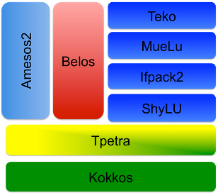
(a) Trilinos solver software stack.

Flexible Solver Interface
ShyLU	Distributed DD preconditioner (FROSch) and
	on-node factorization-based local solvers (Basker, Tacho)
MuLue	Algebraic multigrid solver
Amesos2	Direct solver interfaces (e.g., KLU, PaRDISO, SuperLU, Tacho)
Belos	Krylov solvers (e.g., CG, GMRES, BiCG, and
	their communication-avoiding or pipelined variants)
Ifpack2	Algebraic preconditioners (ILU, relaxation, one-level Schwarz)
Portable Performance
Tpetra	Distributed sparse/dense matrix-vector operations
Kokkos-Kernels	Performance portable on-node graph and sparse/dense matrix operations
Kokkos	C++ programming model for performance portable applications
	on different node architectures (e.g., CPUs, NVIDIA/AMD GPUs)

(b) Linear solver package descriptions.

Figure 2: Trilinos linear solver packages

FROSch [18] implements GDSW type preconditioners within the Trilinos software framework [2], a collection of open-source software packages that can be used as building blocks for developing large-scale scientific applications. Fig. 2 shows the core Trilinos packages for solving linear systems of equations. These packages can be combined to develop a flexible and adaptable solver for large-scale scientific applications. For instance, FROSch has interfaces to these solver packages for solving its local overlapping subdomain and coarse problems: direct solvers (Amesos2 [5]), inexact and preconditioned Krylov solvers (Ifpack2 [23] and Belos [5]), and even a local algebraic multigrid solver or Schwarz methods (MueLu [6] and FROSch [18]). In addition, FROSch can be used as a preconditioner for Belos, which implements Krylov solvers, including variants which can be optimized for the GPU architectures, such as single-reduce, communication-avoiding, and pipelined variants [29].

Furthermore, FROSch builds on the Trilinos software stack, specifically packages that provide the portable performance on different hardware architectures: In particular,

• Kokkos [27] is a C++ performance-portable programming ecosystem. It provides the memory abstraction and functionality to dispatch particular functions for parallel-operations on a specific execution space on a CPU or GPU. This enables portable thread performance on different manycore architectures using a single code base (assuming algorithms are performance portable).

• Kokkos-Kernels [24] is a collection of Kokkos-based kernels for on-node sparse or dense matrix, or graph operations on CPUs and GPU.

• Tpetra [1] implements distributed graph, matrix, and vector operations for CPU and GPU clusters.

Though we focus on the FROSch software stack, this is not the only option for the portable performance stack. For instance, previous studies have compared the performance of the on-node portable layers and individual kernels [27].

V GPU Acceleration

Many of the current high-performance computers are composed of the heterogeneous compute node architectures, i.e., each node consists of multicore CPUs and multiple GPU accelerators. A GPU with a large number of compute cores and a high memory bandwidth is suited for a highly-parallel computation with a regular memory access pattern, while some operations are better suited for CPUs.

This poses both challenges and opportunities for designing high performance sparse linear solvers, including FROSch, where most of the required computational kernels have irregular memory accesses and a small ratio of the computation to the data accesses. As a result, their performance is often bounded not by the computation but by the memory bandwidth, if not by memory latency. In order for the solver to utilize the GPUs well, both the solver and its underlying computational kernels must be carefully designed, and new variants of the algorithms may need to be developed. In this section, we discuss some of the specific approaches taken to improve the performance of FROSch on GPU clusters.

V-A Software Considerations

V-A1 Software Structure

In many scientific and engineering simulations, we often perform the numerical factorization multiple times for a given mesh with the same sparsity structure or need to solve a sequence of linear systems with different right-hand-side vectors. Hence, all the linear solvers in Trilinos have three distinct phases:

1. Symbolic Factorization, given a sparsity structure or a graph, performs all the symbolic analysis and factorization and allocate required GPU memories. Operations such as the symbolic analysis for an LU factorization, computing the level sets for a triangular solve, are done here. This is typically done on a CPU.

2. Numerical Factorization, given numerical values of the input matrix, performs the numerical factorization; in FROSch, this part includes the computation of the coarse basis functions, computing the coarse space matrix, and factoring the overlapping local subdomain and coarse matrices. Steps such as the sparse matrix - sparse matrix multiplication for computing $A_{0}$, numerical factorization of the LU factorization or incomplete factorization are also part of this step. We compute these on the GPUs, when appropriate.

3. Solve Phase, given right-hand-side vector(s), compute the solution to the linear system. The sparse triangular solve for the direct or incomplete factorization of local matrix is done on the GPU as part of this phase.

These distinct phases are critical, especially for GPUs since large parts of the symbolic analysis are difficult to parallelize, and the GPU memory allocations can take a significant amount of time.

V-A2 Lower Precision Preconditioning

Within Trilinos, the software package Belos implements Krylov solvers. It uses the Operator class for applying a preconditioner, including algebraic multigrid (AMG) and domain decomposition (DD) preconditioners, which are implemented in the MueLu and FROSch packages, respectively. These preconditioners are typically constructed from a sparse matrix class, called CrsMatrix.

A new utility function that converts a CrsMatrix object into a new object in half the precision was developed (e.g., if the original matrix is in double precision, then the new matrix will be in single precision), allowing users to construct the preconditioner also in half the precision. The new HalfPrecisionOperator class, which inherits the base Operator class in the working precision and internally holds the operator in half the precision as its member variable, is also implemented. When this new operator is applied to vectors, it internally type-casts the input vectors into half the precision, applies the operator (e.g., preconditioner) in half the precision, and then type-casts the resulting output vector back into the working precision. Though it has the overhead of type-casting, these new capabilities allow users to apply many of the preexisting Trilinos preconditioners in half the precision within the current Trilinos framework. Currently, MueLu and FROSch (whose cost of applying is typically much higher than that of type-casting vectors) have been extended to utilize these new capabilities

V-B Algorithmic Consideration

V-B1 Sparse Direct Matrix Factorization

Most of the theoretical results for DD solvers (including the condition number estimates for the preconditioned matrix) assume the exact solution of the overlapping subdomain and coarse problems. As a result, in practice, DD solver typically use sparse direct solvers.

Sparse direct solvers are a critical component in many scientific applications, and there have been extensive efforts to develop high performance sparse direct solvers [9]. For our experiments, we used SuperLU and Tacho software packages that provide two different approaches to the sparse direct solvers:

• SuperLU [10] implements left-looking sparse LU factorization with partial pivoting. It mainly targets a single CPU core, though it could be linked to threaded BLAS or LAPACK for runing on multicore CPUs. It uses the supernodal block structures of the LU factors in order to exploit the memory hierarchy.

• Tacho [21] is based on multifrontal factorization with pivoting only inside the frontal matrices. The original Tacho used the task programming model of Kokkos. Though the current implementation still uses Kokkos, it exploits the hierarchical parallelism available on a GPU through the combination of level-set scheduling and team-level BLAS/LAPACK like kernels. It also has interface to the vendor-optimized kernels (i.e., NVIDIA’s CuBLAS/cuSolver and AMD’s rocBLAS/rocSolver) to factorize large frontal matrices with GPU streams. Tacho currently supports Cholesky, LDL^T, or LU factorization of a symmetric positive definite, symmetric indefinite, or numerically nonsymmetric matrix but with symmetric pattern, respectively.

V-B2 Sparse Triangular Solve

When a direct sparse matrix factorization is used, the resulting sparse triangular matrix typically has the dense blocks called supernodes. It is possible to exploit this supernodal structure to accelerate the triangular solves. For instance, Kokkos-Kernels implements sparse-triangular solver based on level-set scheduling of supernodal blocks [28]. Working with blocks instead of matrix elements may give several performance advantages on a GPU. For instance, it reduces the height of the level-set trees and the length of the critical path in the parallel execution (e.g., number of kernel launches) of the sparse triangular solve. In addition, it allows the hierarchical parallelization, which fits well to the hierarchical parallelism available on a GPU and can be exposed using team-based kernels in Kokkos-Kernels.

The sparse-triangular solver in Kokkos-Kernels also has an option to perform the partitioned inverse [3] that transforms the sparse triangular solve into a sequence of sparse-matrix vector multiply which provides more parallelism than the standard substitution-based algorithm [28].

V-B3 Incomplete Local Solver

Though DD theory is based on exact solution of the local subdomain and coarse problems, an inexact local solver may work well in practice, in particular, if its application is somewhat spectrally equivalent to applying an exact solver. In this paper, we explore inexact local solver based on level-based incomplete sparse LU factorization. Though several parallel ILU implementations have been proposed, the standard paralelization scheme for the ILU and spares-triangular solve is based on the level-set scheduling [4]. In Trilinos, these are implemented as SpILU and SpTRSV in Kokkos Kernels [24].

Though incomplete factorization leads to a fewer fills and may expose more parallelism, it may still not provide enough parallelism to utilize a GPU. To expose more parallelism, iterative variants of sparse approximate factorization and of sparse triangular solver are proposed [8]. It uses Jacobi iterations to approximate each entries of the LU factors or to approximately solve the linear system with a sparse triangular matrix. Though each iteration requires the about same number of floating point operations as the standard algorithms, this variant has significantly more parallelism. As a result, when the solver needs a small number of iterations to obtain the solution of the desired approximation accuracy (our default is five iterations for both), it may obtain much shorter time to solution on a GPU. In Trilinos, these are implemented as FastILU and FastSpTRSV [7].

VI Discussion

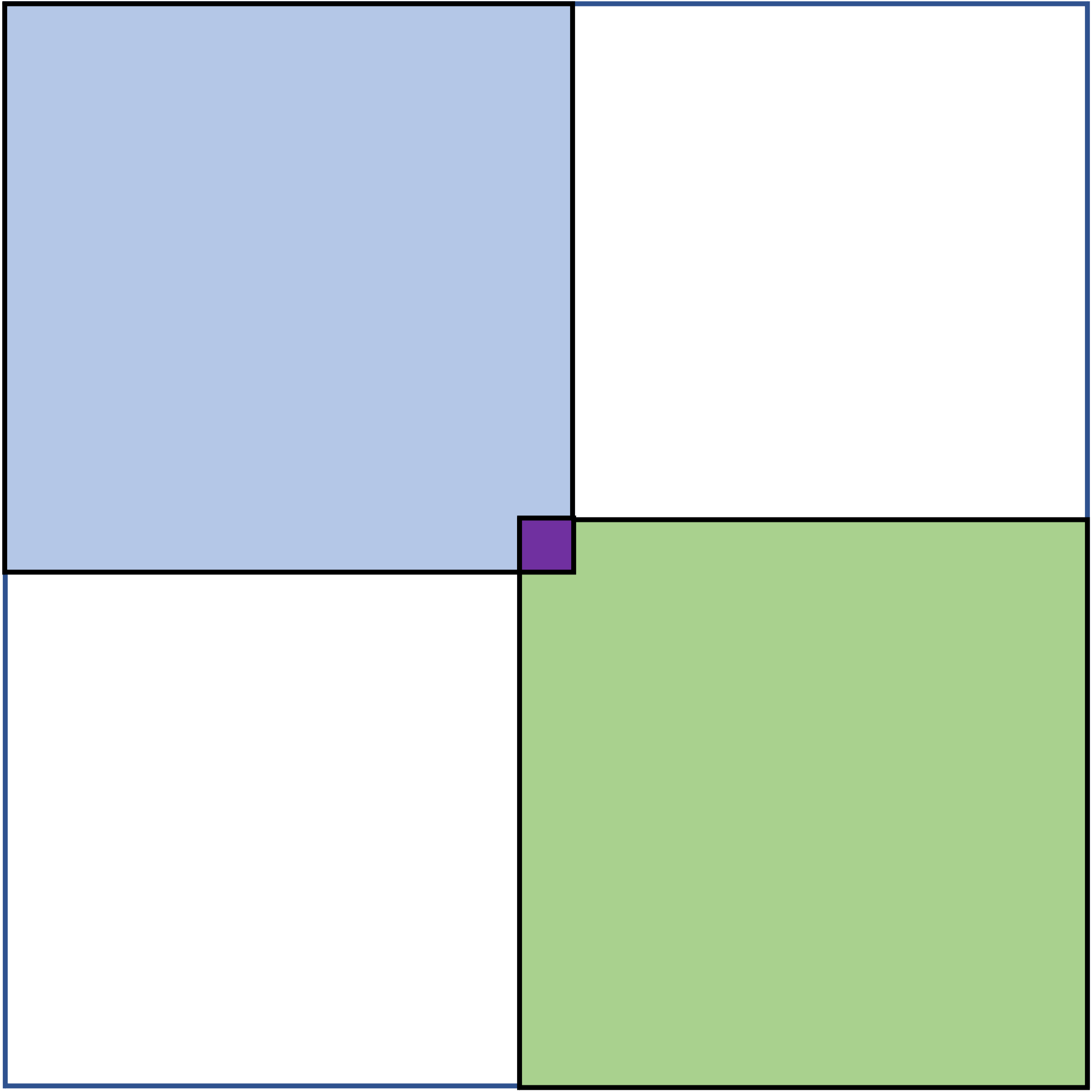
(a) two subdomains.

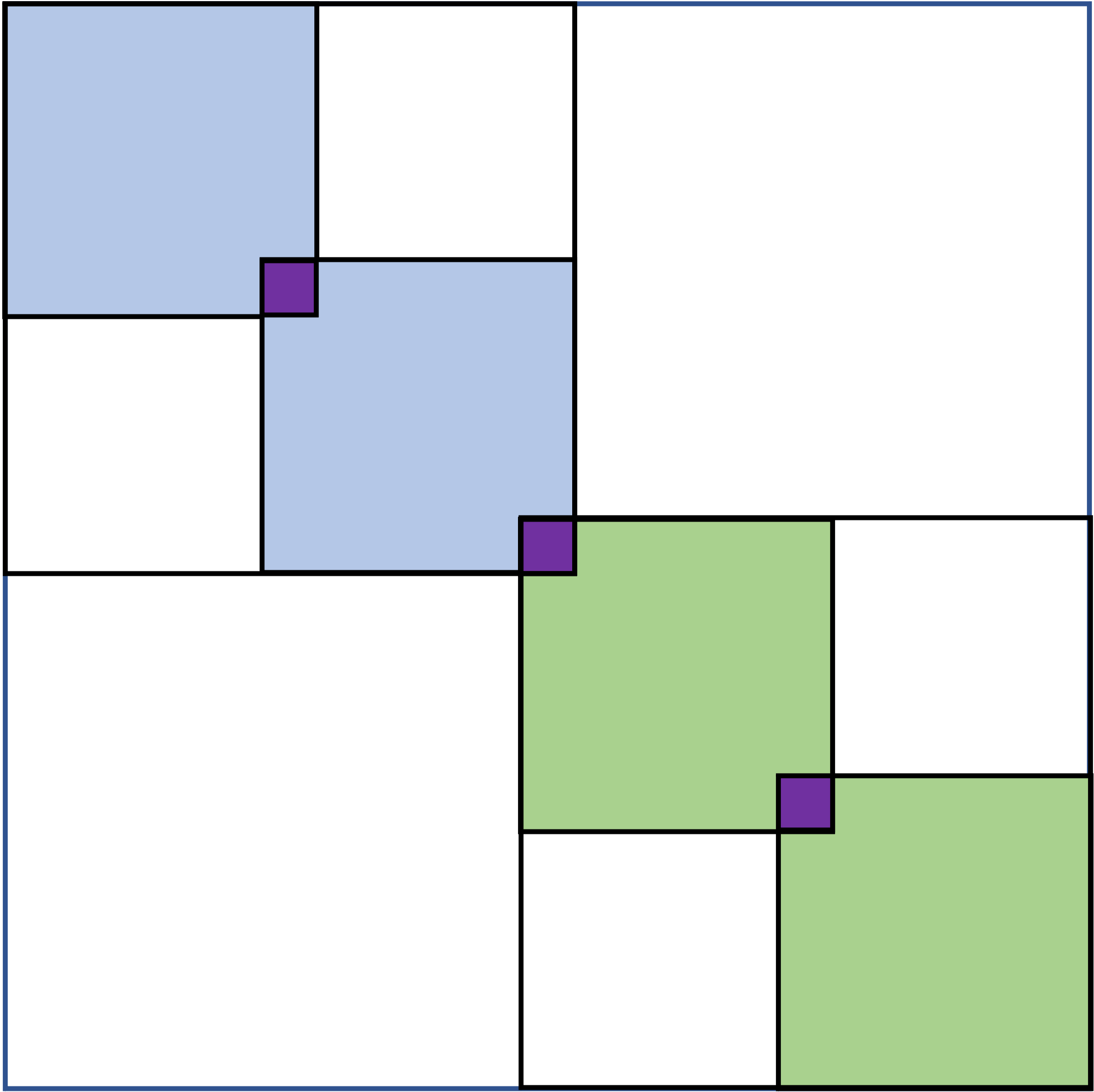
(b) Four subdomains.

Figure 3: Overlapping domain decomposition into two or four subdomains (e.g., one or two MPIs on each of two GPUs). Instead of assigning two large subdomains to two GPUs (left), we assign four small subdomains to two GPUs (right).

Current heterogeneous node architectures typically have more CPU cores than GPUs on each node (e.g., each node of the Summit supercomputer has 42 IBM Power9 CPU cores and 6 NVIDIA V100 GPUs). Such a heterogeneous node architecture poses challenges for a node-to-node performance comparison of the DD solver on CPUs and with GPUs. This is because, in most cases, the computational complexity of the local sparse solver increases more than linearly to the local matrix size. For example, for a 3D problem, when the nested dissection [14] is used to permute the local matrix with dimension of $n_{i}$, the sparse direct factorization and corresponding sparse-triangular solve of the local problem typically have the computational complexities of $\mathcal{O}(n_{i}^{2})$ and $\mathcal{O}(n_{i}^{4/3})$, respectively. As a result, for our strong parallel-scale studies, the computational cost of the DD solver decreases superlinearly with the number of MPI processes. Since each node typically has fewer GPUs than CPU cores, if we launch one MPI process on each CPU core for CPU runs and one MPI process on each GPU for GPU runs (these are the most common setups in practice), each process has a much smaller computational cost for the CPU runs than for the GPU runs.

Moreover, the condition number of the matrix preconditioned with a GDSW preconditioner is bounded as follows:

$$\kappa\left(M_{\rm GDSW}^{-1}A\right)\leq C\left(1+\frac{H}{\delta}\right)\left(1+\log\left(\frac{H}{h}\right)\right)^{2};$$

where $H$ is the maximum diameter of the subdomains and $\delta$ is the width of the overlap cf. [11]. Hence, the condition number will decrease with a smaller subdomain size ($H/h$), e.g., as the number of subdomains increases with a fixed problem size.

For our experiments, we used NVIDIA Multi-Process Service (MPS) to run multiple MPI processes on each GPU (see Fig. 3). Compared to having just one process on each GPU, this not only reduces the computational and storage costs of the DD solver, but it may also improve the condition number of the preconditioned matrix, and hence the convergence rate of the Krylov solver. It is possible to obtain the same decomposition by having multiple subdomains per MPI and using GPU streams. However, this will require significant algorithmic innovations and software efforts for a two-level solver. Though it may not be optimal, MPS allows us to run the existing code without these code changes and can provide significant performance gain running multiple subdomains per GPU.

VII Experimental Setup

For all of our performance results presented in this paper, we used the “reduced” GDSW coarse space with an algebraic overlap of one . Then, as our Krylov solver, the single-reduce variant [30] of the Generalized Minimum Residual (GMRES) method [25] was used, which is a popular Krylov method for solving nonsymmetric linear systems of equations. We used the restart length of 30, and considered GMRES to be converged when the residual norm is reduced by a factor of $10^{-7}$. Finally, we focused on solving 3D elasticity problems in this paper. Though there are several other preconditioning options in FROSch, since our focus is on the performance comparison, and not on the numerical study of GDSW, these setups provide representative performance of FROSch.

We present performance results on the Summit Supercomputer at Oak Ridge Leadership Computing Facility. Each node of Summit has 42 IBM Power9 CPU cores and 6 NVIDIA V100 GPUs. Unless specified otherwise, for our CPU runs, we launched 42 MPI processes on each node (one MPI per CPU core), while for our GPU runs, we used NVIDIA Multi-Process Service (MPS) to run up to 7 MPI processes on each GPU (up to 42 MPI processes per node). The codes were compiled using CUDA 10.2.89 and GCC 7.5.0, and linked to the vendor-optimized libraries, NVIDIA’s CUBLAS, CuSparse on GPUs, and IBM’s Engineering and Scientific Subroutine Library (ESSL) 6.3.

VIII Performance Results

# comp. nodes		1	2	4	8	16
matrix size		375K	750K	1.5M	3M	6M
CPU		2.03 (75)	2.07 (69)	1.87 (61)	1.95 (58)	2.48 (69)
GPU	$n_{p}$/gpu = 1	1.43 (47)	1.52 (53)	2.82 (77)	2.44 (68)	2.61 (75)
	2	1.03 (46)	1.36 (65)	1.37 (60)	1.52 (65)	1.98 (86)
	4	0.93 (59)	0.91 (53)	0.98 (59)	1.33 (77)	1.21 (66)
	6	0.67 (46)	0.99 (65)	0.92 (57)	0.91 (57)	0.95 (57)
	7	1.03 (75)	1.04 (69)	0.90 (61)	0.97 (58)	1.18 (69)
speedup		$\mathbf{2.0\times}$	$\mathbf{2.0\times}$	$\mathbf{2.1\times}$	$\mathbf{2.0\times}$	$\mathbf{2.1\times}$

(a) SuperLU.
 

# comp. nodes		1	2	4	8	16
matrix size		375K	750K	1.5M	3M	6M
CPU		1.60 (75)	1.63 (69)	1.49 (61)	1.51 (58)	1.90 (69)
GPU	$n_{p}$/gpu = 1	1.17 (47)	1.37 (53)	1.92 (77)	1.78 (68)	2.21 (75)
	2	0.79 (46)	1.14 (65)	1.05 (60)	1.18 (65)	1.70 (86)
	4	0.85 (59)	0.81 (53)	0.78 (59)	1.22 (77)	1.19 (66)
	6	0.60 (46)	0.86 (65)	0.75 (57)	0.84 (57)	0.91 (57)
	7	0.99 (75)	0.93 (69)	0.82 (61)	0.93 (58)	1.22 (69)
speedup		$\mathbf{1.6\times}$	$\mathbf{1.8\times}$	$\mathbf{1.8\times}$	$\mathbf{1.6\times}$	$\mathbf{1.6\times}$

(b) Tacho.

TABLE II: Total iteration time in seconds and Iteration count for Weak-scale 3D elasticity problems on Summit.

VIII-A Exact Local Solvers

In this section, we study the performance of FROSch using exact solution of the local overlapping subdomain and coarse space problems. The nested dissection ordering from Metis [20] was used to reduce the number of fills in the LU factors, and also to expose more parallelism. We used either SuperLU or Tacho to factor our local and coarse matrices on CPUs or GPUs, respectively. To apply the preconditioner on a GPU with the LU factors computed by SuperLU, the supernodal sparse-triangular solver [28] from Kokkos-Kernels was used, while on CPU, we used the SuperLU’s internal triangular solver since Kokkos-Kernels solver is designed to exploit the manycore architectures and is not suited on a single CPU core. With Tacho, we used its internal sparse-triangular solver for both CPU and GPU runs. We did not use the partitioned inverse, and all the sparse-triangular solvers, either on a CPU or on a GPU, are numerically equivalent.

Table II shows the the weak-parallel scaling of the total iteration time required for the solution convergence, where the local problem size on each compute node is fixed and the global matrix size grows linearly to the number of the compute nodes. We used MPS to run multiple MPI processes on each GPU. As we discussed in Section VII, with the direct factorization of of the local overlapping subdomain matrix, the resulting sparse-triangular solve has the computational cost that scales superlinearly to the size of the local matrix. Hence, as we map more MPI processes on each GPU using MPS, the local subdomain becomes smaller, and the iterative solution time is reduced, significantly (with speedups of $1.3\sim 2.7\times$). Overall, using GPUs, the solution time was reduced by a factor of around $2\times$, compared to the CPU runs.

In some applications, the setup time can also take a significant share of the total simulation time. Hence, we now study the numerical setup time of FROSch. Fig. 5 shows the breakdown of the numerical setup time on a single compute node of Summit. As we expect, especially on CPUs, a significant part of the numerical setup time is spent by the sparse direct solver. For both CPU and GPU runs with SuperLU, the local overlapping and coarse matrices are factored on CPU, and the factorization time are the same on CPUs and with GPUs. On the other hand, Tacho can exploit the GPU, and the local factorization time was reduced for the GPU run by $2.4\times$. This is the first benefit of using GPUs. Unfortunately, we also see that some of the setup time beside the sparse direct solver is running slower with GPUs (“black” part of the bar), and a significant amount of time is spent setting up the Kokkos-Kernels sparse-triangular solve with SuperLU:

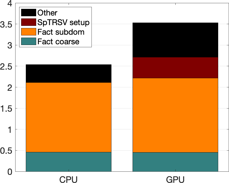
(a) SuperLU

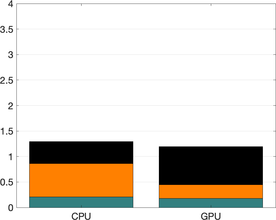
(b) Tacho

Figure 5: Breakdown of the numerical setup time on one node of Summit ($n=375$K on 42 MPI processes).

# comp. nodes		1	2	4	8	16
matrix size		375K	750K	1.5M	3M	6M
CPU		2.5	3.0	3.3	3.8	3.6
GPU	$n_{p}$/gpu = 1	60.0	71.5	70.9	85.6	85.1
	2	22.9	22.3	26.1	26.9	25.8
	4	8.4	9.4	9.1	9.8	10.2
	6	5.5	5.2	5.2	6.2	6.3
	7	3.5	4.2	4.8	5.4	5.4
slowdown		$\mathbf{1.4\times}$	$\mathbf{1.4\times}$	$\mathbf{1.5\times}$	$\mathbf{1.4\times}$	$\mathbf{1.5\times}$

(a) SuperLU.
 

# comp. nodes		1	2	4	8	16
matrix size		375K	750K	1.5M	3M	6M
CPU		1.3	1.6	1.7	1.8	1.9
GPU	$n_{p}$/gpu = 1	3.2	3.5	3.9	5.4	5.6
	2	2.1	2.3	2.9	3.3	3.4
	4	1.4	1.8	2.1	2.2	2.3
	6	1.5	1.6	1.7	2.0	2.3
	7	1.2	1.6	1.7	2.0	2.2
slowdown		$\mathbf{0.9\times}$	$\mathbf{1.0\times}$	$\mathbf{1.0\times}$	$\mathbf{1.1\times}$	$\mathbf{1.1\times}$

(b) Tacho.

TABLE III: Numerical Setup Time in seconds for Weak-scale 3D elasticity problems on Summit. Number of MPI process per GPU changes between every GPU row from 1 to 7. This improves the numerical setup time up to 17x and 3x for SuperLU and Tacho on GPU runs. The GPU runs are slightly slower than CPU runs in this phase.

• SuperLU performs partial pivoting during its numerical factorization. This ensures the numerical stability of the solver, but the sparsity structures of the LU factors depend on the numerical values. As a result there is very little work that can be reused from the symbolic factorization. For instance, with SuperLU, both the symbolic and numerical setups for the Kokkos-Kernels sparse-triangular solver need to be performed after each numerical factorization, which takes up significant part of the difference between the setup times on CPUs and with GPUs in the plot.

• On the other hand, Tacho performs the pivoting only within its frontal matrices and given the same sparsity structure of the input matrices, the sparsity structures of the LU factors stay the same, allowing us to reuse the symbolic setup for the numerical factorization of different matrices. In addition, Tacho can utilize the GPU. Overall, we see similar numerical setup times of Tacho on CPUs and with GPUs.

Table III compares the the weak-scaling numerical setup time of FROSch using up to 672 CPU cores and 96 GPUs. As we discussed in Section VII, the computational cost for factoring the local overlapping subdomain scales superlinearly to the size of the local matrix. Hence, similar to the iterative solution time, the numerical setup time was reduced significantly using MPS (obtaining speedups of $15\sim 17\times$ with SuperLU and $2\sim 3\times$ with Tacho). Running multiple MPI processes on each GPU also reduced the memory required to store the LU factors, enabling the solution of a larger linear system.

Overall, using Tacho, the total solution time (the sum of setup and solve time for solving a single linear system) was $1.1\sim 1.8\times$ faster with GPUs. If the application requires to solve a sequence of linear systems (the same matrix $A$ but with different right-hand-side $b$ in sequence), then the cost of the numerical factorization can be amortized over the multiple solves, and speedups closer to $2\times$ can be obtained.

(a) Numerical setup time.

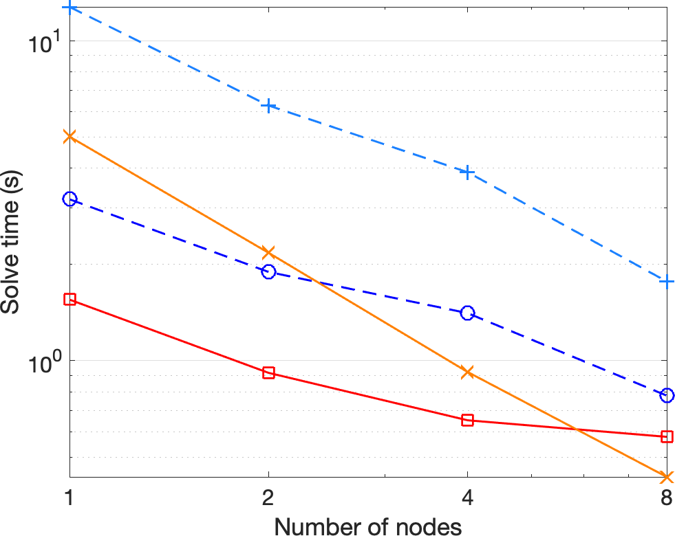
(b) Solve time.

Figure 7: Strong parallel scaling with 3D elasticity ($n=1$M).

To summarize our studies with the exact solver, Fig. 7 shows the strong parallel-scaling results, where either 6 or 42 MPI processes were used on each node. For our CPU runs with 6 MPI processes per node, we linked Tacho with the threaded version of ESSL and used 7 threads for each MPI process. We clearly see the advantage of having 42 MPI processes on each node for both CPU and GPU runs. Overall, the GPUs can provide speedups for both setup and solve time as long as the local matrix sizes are large enough.

VIII-B Approximate Local Solvers

VIII-B1 Incomplete LU Factorization

ILU level 0 1 2 3 CPU No 1.5 1.9 3.0 4.8 ND 1.6 2.6 4.4 7.4 GPU KK(No) 1.4 1.5 1.8 2.4 KK(ND) 1.7 2.0 2.9 5.2 Fast(No) 1.5 1.6 2.1 3.2 Fast(ND) 1.5 1.7 2.5 4.5 speedup $\mathbf{1.0\times}$ $\mathbf{1.2\times}$ $\mathbf{1.4\times}$ $\mathbf{1.5\times}$

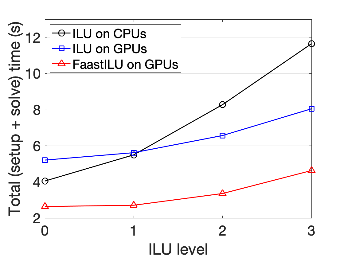
(a) Setup (table on left) and total time (figure on right).
 

ILU level		0	1	2	3
CPU	No	2.55 (158)	3.60 (112)	5.28   (99)	6.85   (88)
	ND	4.17 (227)	5.36 (134)	6.61 (105)	7.68   (88)
GPU	KK(No)	3.81 (158)	4.12 (112)	4.77   (99)	5.65   (88)
	KK(ND)	2.89 (227)	4.27 (134)	5.57 (105)	6.36   (88)
	Fast(No)	1.14 (173)	1.11 (141)	1.26 (134)	1.43 (126)
	Fast(ND)	1.49 (227)	1.15 (137)	1.10 (109)	1.22 (100)
speedup		$\mathbf{2.2\times}$	$\mathbf{3.2\times}$	$\mathbf{4.3\times}$	$\mathbf{4.8\times}$

(b) Solve time (iteration count).

TABLE IV: Performance of FROSch for 3D elasticity problems on one Summit node ($n=648$K on 42 MPI processes) using local Kokkos-Kernels ILU (KK) or FastILU (Fast) and no reordering (No) or nested dissection (ND).

We now study the effects of using an incomplete LU (ILU) factorization as our local solver on the performance of FROSch. For these experiments, we used level-based ILU($k$) as local solver only for solving the local overlapping subdomain problems, while Tacho was used for computing the basis function and for solving the coarse problem. The inexact solvers reduce the required storage cost, and hence, we are solving larger linear systems in this section, compared to those solved in Section VIII-A.

Table 8(a) shows the effects of the number of ILU levels, $k$, on the numerical setup time. Besides SpILU and SpTRSV (based on level-set scheduling), we also show the performance of their iterative variants, FastILU and FastSpTRSV, where we performed three and five Jacobi iterations, respectively. As we increase the level (and the computation required to compute ILU factors increases), the speedup gained using the GPUs for the numerical setup time increased.

Table 8(b) shows the total iteration time with increasing levels for ILU. FastILU computes approximation to the ILU factors, and FastSpTRSV solves the triangular system, approximately. As a result, compared to SpILU, GMRES required more iterations to converge using FastILU. However, they provide more parallelism, which the GPU can exploit. Overall, GMRES had the fastest time to solution using the iterative variants with the speedups of $2.8\sim 4.4\times$.

# comp. nodes		1	2	4	8	16
matrix size		648K	1.2M	2.6M	5.2M	10.3M
CPU		1.9	2.2	2.4	2.4	2.6
GPU	KK	1.4	2.0	2.2	2.4	2.8
	Fast	1.5	2.2	2.3	2.5	2.8
speedup		$\mathbf{1.3\times}$	$\mathbf{1.0\times}$	$\mathbf{1.0\times}$	$\mathbf{1.0\times}$	$\mathbf{0.9\times}$

(a) Setup time (s).
 

# comp. nodes		1	2	4	8	16
matrix size		648K	1.2M	2.6M	5.2M	10.3M
CPU		4.0 (119)	3.8 (110)	3.7 (105)	3.3   (97)	4.1 (109)
GPU	KK	4.3 (119)	3.9 (110)	4.8 (105)	4.3   (97)	4.9 (109)
	Fast	1.2 (154)	1.0 (133)	1.1 (130)	1.3 (117)	1.6 (131)
speedup		$\mathbf{3.3\times}$	$\mathbf{3.8\times}$	$\mathbf{3.4\times}$	$\mathbf{2.5\times}$	$\mathbf{2.6\times}$

(b) Solve time (s) (iteration count).

TABLE V: Weak scaling Parallel Performance (42 MPIs on each node) of 3D elasticity problems on Summit, using ILU(1) as local subdomain solvers.

Finally, Table V shows weak-scaling results using the inexact ILU(1) local solver on up to 672 CPU cores and 96 GPUs. For all these experiments, we used the original matrix ordering since the matrix reordering did not improve the performance significantly, while it could increase the iteration count. Even with the inexact local solver, the iteration counts were almost independent of the number of subdomains. It can be seen in Table V that even with the higher iteration count, the inexact (Fast) option is faster than the exact triangular solve (KK). We see $3.1\sim 4.4\times$ speedups using the iterative variants on GPUs. We also observe $2.5\sim 3.8\times$ speedup using GPUs. The setup times are nearly the same on CPUs and GPUs with ILU(1) on multiple nodes.

VIII-B2 Single-precision FROSch

# comp. nodes		1	2	4	8	16
matrix size		375K	750K	1.5M	3M	6M
CPU	double	2.5	3.0	3.3	3.8	3.6
	single	1.8	2.2	2.3	2.6	2.6
	speedup	$1.4\times$	$1.4\times$	$1.4\times$	$1.5\times$	$1.4\times$
GPU	double	3.5	4.2	4.8	5.6	5.4
	single	2.6	3.2	3.4	4.0	4.0
	speedup	$1.3\times$	$1.3\times$	$1.4\times$	$1.4\times$	$1.4\times$

(a) SuperLU.
 

# comp. nodes		1	2	4	8	16
matrix size		375K	750K	1.5M	3M	6M
CPU	double	1.3	1.6	1.7	1.8	1.9
	single	1.0	1.2	1.3	1.4	1.4
	speedup	$1.3\times$	$1.3\times$	$1.3\times$	$1.3\times$	$1.4\times$
GPU	double	1.2	1.6	1.7	2.0	2.2
	single	1.0	1.3	1.4	1.7	2.0
	speedup	$1.2\times$	$1.2\times$	$1.2\times$	$1.2\times$	$1.1\times$

(b) Tacho.

TABLE VI: Numerical Setup Time in seconds, using single or double precision FROSch: for Weak-scale 3D elasticity problems on Summit.

# comp. nodes		1	2	4	8	16
matrix size		375K	750K	1.5M	3M	6M
CPU	double	2.03 (75)	2.07 (69)	1.87 (61)	1.95 (58)	2.48 (69)
	single	1.89 (76)	1.60 (69)	1.71 (62)	1.75 (58)	2.37 (69)
	speedup	$1.0\times$	$1.3\times$	$1.1\times$	$1.1\times$	$1.0\times$
GPU	double	1.03 (75)	1.04 (69)	0.90 (61)	0.97 (58)	1.18 (69)
	single	1.01 (75)	1.03 (69)	0.98 (62)	1.10 (58)	1.28 (69)
	speedup	$1.0\times$	$1.0\times$	$0.9\times$	$0.9\times$	$0.9\times$

(a) SuperLU.
 

# comp. nodes		1	2	4	8	16
matrix size		375K	750K	1.5M	3M	6M
CPU	double	1.60 (75)	1.63 (69)	1.49 (61)	1.51 (58)	1.90 (69)
	single	1.11 (76)	1.13 (69)	1.02 (62)	1.04 (58)	1.30 (69)
	speedup	$1.4\times$	$1.4\times$	$1.4\times$	$1.4\times$	$1.5\times$
GPU	double	0.99 (75)	0.93 (69)	0.82 (61)	0.93 (58)	1.22 (69)
	single	1.00 (75)	0.92 (69)	0.84 (62)	0.93 (58)	1.21 (69)
	speedup	$1.0\times$	$1.0\times$	$1.0\times$	$1.0\times$	$1.0\times$

(b) Tacho.

TABLE VII: Total iteration time and Iteration count, using double or single precision FROSch for Weak-scale 3D elasticity problems on Summit.

Even though typical scientific applications require double precision accuracy, some emerging hardware delivers lower-precision arithmetic at higher performance. There are other machines that provide the same performance for double and single precision arithmetic. However, even in that case, using a lower-precision arithmetic reduces the required amount of data transfer. Since the performance of the sparse solver is often limited by the memory bandwidth, reducing the required communication volume alone could reduce the solver time.

Table VII shows the performance results, where FROSch in single precision is used to precondition GMRES in double precision. For these particular problems, the setup time was reduced using single-precision FROSch, while the number of iterations required for the convergence to same accuracy as double precision use cases is maintained. Specifically, using single precision, both on 672 CPU cores and 96 GPUs, we observe $1.3\sim 1.5\times$ speedup in SuperLU based setup, while we observe $1.1\sim 1.4\times$ speedup in Tacho based setup. We do not see a benefit in solve times when using single precision (Table VII). Nevertheless, GMRES converges in similar number of iterations when using single or double precision preconditioner.

VIII-C Summary of Key Results

Using multiple subdomains per GPU improves the performance considerably. In terms of the setup time using a direct factorization for the subdomain solver, GPU-based factorization in Tacho provides a distinct advantage over CPU-based SuperLU. There is no distinct advantage in the solve time on the GPUs when using SuperLU and Kokkos Kernels combination or using Tacho. Incomplete factorizations allow us to solve larger problems. Though we do not see noticeable difference in performance over direct factorization due to the trade-off between number of iterations and setup/solve times, the solve time was reduced using GPUs. Iterative incomplete factorizations and triangular solve result in significant speedup compared to the standard incomplete factorizations even with increased number of iterations. Using lower precision computations allows us to solve a larger linear system, and improved the setup time though not the solve time.

IX Conclusion

We presented FROSch, which implements the GDSW algorithm for GPU cluster within Trilinos software framework. Our performance results on Summit supercomputer with NVIDIA V100 GPUs demonstrated the potential of FROSch: with GPUs, the numerical setup times remain about the same as that on CPUs, while the solve time can be reduced by factors of around $2\times$. We presented a thorough experimental study varying several solver options from two direct solvers, incomplete factorization techniques with different level of fill and different orderings, inexact factorizations and the use of lower precision arithmetic. Though we only showed the performance results with NVIDIA GPUs, our implementation is portable to other GPUs through the use of Kokkos. We plan to study performance of FROSch with AMD GPUs.

References

- [1] Tpetra parallel linear algebra. https://trilinos.github.io/tpetra.html.
- [2] The Trilinos Project Website. https://trilinos.github.io.
- [3] F. L. Alvarado, A. Pothen, and R. Schreiber. Highly parallel sparse triangular solution. In Graph Theory and Sparse Matrix Computation. The IMA Volumes in Mathematics and its Applications, chapter 56, pages 141–157. Springer, New York, NY, 1993.
- [4] E. Anderson and Y. Saad. Solving sparse triangular linear systems on parallel computers. Int. J. High Speed Comput., 1:73–95, 1989.
- [5] E. Bavier, M. Hoemmen, S. Rajamanickam, and H. Thornquist. Amesos2 and Belos: Direct and iterative solvers for large sparse linear systems. Scientific Programming, 20, 2012.
- [6] L. Berger-Vergiat, C. A. Glusa, J. J. Hu, M. Mayr, A. Prokopenko, C. M. Siefert, R. S. Tuminaro, and T. A. Wiesner. MueLu user’s guide. Technical Report SAND2019-0537, Sandia National Laboratories, 2019.
- [7] E. G. Boman, A. Patel, E. Chow, and S. Rajamanickam. FastILU: Finegrained asynchronous iterative ILU. Technical Report 2016-12066C 649521, Sandia National Labs, 2016. presentation at the SIAM Applied Linear Algebra 2016.
- [8] E. Chow and A. Patel. Fine-grained parallel incomplete LU factorization. SIAM J. Sci. Comput., 37(2):C169–C193, 2015.
- [9] T. A. Davis, S. Rajamanickam, and W. M. Sid-Lakhdar. A survey of direct methods for sparse linear systems. Acta Numerica, 25:383–566, 2016.
- [10] J. W. Demmel, S. C. Eisenstat, J. R. Gilbert, X. S. Li, and J. W. H. Liu. A supernodal approach to sparse partial pivoting. SIAM J. Matrix Anal. Appl., 20(3):720–755, 1999.
- [11] C. R. Dohrmann, A. Klawonn, and O. B. Widlund. A family of energy minimizing coarse spaces for overlapping Schwarz preconditioners. In Domain Decomposition Methods in Science and Engineering XVII, pages 247–254. Springer Berlin Heidelberg, 2008.
- [12] C. R. Dohrmann and O. B. Widlund. On the design of small coarse spaces for domain decomposition algorithms. SIAM J. Sci. Comput., 39(4):A1466–A1488, 2017.
- [13] V. Dolean, P. Jolivet, and F. Nataf. An Introduction to Domain Decomposition Methods: Algorithms, Theory, and Parallel Implementation. Society for Industrial and Applied Mathematics, 2015.
- [14] A. George. Nested dissection of a regular finite element mesh. SIAM J. Numer. Anal., 10(2):345–363, 1973.
- [15] A. Heinlein, C. Hochmuth, and A. Klawonn. Reduced dimension GDSW coarse spaces for monolithic Schwarz domain decomposition methods for incompressible fluid flow problems. Int. J. Numer. Methods Eng., 121(6):1101–1119, 2020.
- [16] A. Heinlein, C. Hochmuth, and A. Klawonn. Fully algebraic two-level overlapping Schwarz preconditioners for elasticity problems. In Numerical Mathematics and Advanced Applications ENUMATH 2019, pages 531–539. Springer International Publishing, 2021.
- [17] A. Heinlein, A. Klawonn, J. Knepper, and O. Rheinbach. Adaptive GDSW coarse spaces for overlapping Schwarz methods in three dimensions. SIAM J. Sci. Comput., 41(5):A3045–A3072, 2019.
- [18] A. Heinlein, A. Klawonn, S. Rajamanickam, and O. Rheinbach. FROSch: A Fast and Robust Overlapping Schwarz domain decomposition preconditioner based on Xpetra in Trilinos. In Domain Decomposition Methods in Science and Engineering XXV, pages 176–184, 2020.
- [19] A. Heinlein, O. Rheinbach, and F. Röver. Parallel scalability of three-level FROSch preconditioners to 220000 cores using the Theta supercomputer. SIAM J. Sci. Comput. (Copper Mountain Conference on Iterative and Multigrid Methods), pages S173–S198, 2021.
- [20] G. Karypis. METIS: A software package for partitioning unstructured graphs, partitioning meshes, and computing fill-reducing orderings of sparse matrices. Technical report, 2013.
- [21] K. Kim, H. C. Edwards, and S. Rajamanickam. Tacho: Memory-scalable task parallel sparse cholesky factorization. In IEEE International Parallel and Distributed Processing Symposium Workshops, 2018.
- [22] L. Luo, C. Yang, Y. Zhao, and X. C. Cai. A scalable hybrid algorithm based on domain decomposition and algebraic multigrid for solving partial differential equations on a cluster of CPU/GPUs. In international workshop on GPUs and scientific applications, 2011.
- [23] A. Prokopenko, C. M. Siefert, J. J. Hu, M. Hoemmen, and A. Klinvex. Ifpack2 User’s Guide 1.0. Technical Report SAND2016-5338, Sandia National Labs, 2016.
- [24] S. Rajamanickam, S. Acer, L. Berger-Vergiat, V. Q. Dang, N. D. Ellingwood, E. Harvey, B. Kelley, C. R. Trott, J. J. Wilke, and I. Yamazaki. Kokkos Kernels: Performance portable sparse/dense linear algebra and graph kernels. CoRR, abs/2103.11991, 2021.
- [25] Y. Saad and M. Schultz. GMRES: A generalized minimal residual algorithm for solving nonsymmetric linear systems. SIAM J. Sci. Comput., 7:856–869, 1986.
- [26] B. F. Smith, P. E. Bjørstad, and W. D. Gropp. Domain decomposition: parallel multilevel methods for elliptic partial differential equations. Cambridge University Press, 1996.
- [27] C. Trott, L. B.-Vergiat, D. Poliakoff, S. Rajamanickam, D. L.-Grandie, J. Madsen, N. Awar, M. Gligoric, G. Shipman, and G. Womeldorff. The Kokkos ecosystem: Comprehensive performance portability for high performance computing. Comput Sci Eng, 23(5):10–18, 2021.
- [28] I. Yamazaki, S. Rajamanickam, and N. Ellingwood. Performance portable supernode-based sparse triangular solver for manycore architectures. In International Conference on Parallel Processing, 2020.
- [29] I. Yamazaki, S. Thomas, M. Hoemmen, E. Boman, K. Świrydowicz, and J. Elliott. Low-synchronization orthogonalization schemes for s-step and pipelined Krylov solvers in Trilinos. In Proceedings of SIAM Conference on Parallel Processing for Scientific Computing, pages 118–128, 2020.
- [30] K. Świrydowicz, J. Langou, S. Ananthan, U. Yang, and S. Thomas. Low synchronization Gram–Schmidt and generalized minimal residual algorithms. Num. Lin. Alg. Appl., 28(2):e2343, 2021.
- [31] Jakub Šístek and Tomáš Oberhuber. Acceleration of a parallel BDDC solver by using graphics processing units on subdomains. The International Journal of High Performance Computing Applications, page 10943420221136873, November 2022. Publisher: SAGE Publications Ltd STM.