Abstract

Mediation analysis is widely used in health science research to evaluate the extent to which an intermediate variable explains an observed exposure-outcome relationship. However, the validity of analysis can be compromised when the exposure is measured with error. Motivated by the Health Professionals Follow-up Study (HPFS), we investigate the impact of exposure measurement error on assessing mediation with a survival outcome, based on the Cox proportional hazards outcome model. When the outcome is rare and there is no exposure-mediator interaction, we show that the uncorrected estimators of the natural indirect and direct effects can be biased into either direction, but the uncorrected estimator of the mediation proportion is approximately unbiased as long as the measurement error is not large or the mediator-exposure association is not strong. We develop ordinary regression calibration and risk set regression calibration approaches to correct the exposure measurement error-induced bias when estimating mediation effects and allowing for an exposure-mediator interaction in the Cox outcome model. The proposed approaches require a validation study to characterize the measurement error process. We apply the proposed approaches to the HPFS (1986–2016) to evaluate extent to which reduced body mass index mediates the protective effect of vigorous physical activity on the risk of cardiovascular diseases, and compare the finite-sample properties of the proposed estimators via simulations.

Key words: Bias analysis; mediation proportion; natural indirect effect; regression calibration; time-to-event data

1 Introduction

Mediation analysis is a popular statistical tool to disentangle the role of an intermediate variable, otherwise known as a mediator, in explaining the causal mechanism from an exposure to an outcome. It requires the decomposition of the total effect (TE) from the exposure on the outcome into a natural indirect effect (NIE) that works through the mediator and a natural direct effect (NDE) that works around the mediator (Baron and Kenny, 1986). Oftentimes, the mediation proportion (MP), defined as the ratio of NIE and TE, is employed to measure the extent to which the mediator explains the underlying exposure-outcome relationship. The NIE, NDE, TE, and MP are four effect measures of primary interest in mediation analysis (Cheng et al., 2022). In health sciences, mediation analysis is often used to analyze cross-sectional data with a continuous or a binary outcome. Recent advances have extended mediation analysis to accommodate survival or time-to-event outcomes subject to right censoring (e.g., Lange and Hansen, 2011; VanderWeele, 2011; Wang and Albert, 2017).

Health science data are usually measured with error, which may compromise the validity of statistical analyses. The problem of measurement error in mediation analysis with a continuous/binary outcome has been previously studied, and a literature review on methods that correct for the bias due to an error-prone exposure, mediator, or outcome can be found in Cheng et al. (2023). These previous studies, however, have not fully addressed challenges due to measurement error in mediation analysis with a survival outcome. One exception is Zhao and Prentice (2014), who developed regression calibration approaches to address estimation bias due to measurement error in the mediator, under the strong assumption that the measurement error process is known or can be accurately informed by prior information.

In this article, we investigate the implications of exposure measurement error in mediation analysis with a survival outcome, under a linear measurement error model for the mediator and a Cox proportional hazards regression for the survival outcome. Our methods are motivated by the need to address mismeasured exposure in evaluating the effect of vigorous physical activity through body mass index (BMI) on the risk of cardiovascular diseases in the Health Professionals Follow-up Study (HPFS) (Chomistek et al., 2012). In HPFS, physical activity data was assessed through a self-administered physical activity questionnaire, whose accuracy was validated by physical activity diaries in the HPFS validation study. The measurement based on a physical activity diary is expensive but much more accurate, which is considered as gold-standard for assessing physical activity (Chasan-Taber et al., 1996). As is shown in Figure 1, the questionnaire-based measurements are different from the gold-standard diary-based measurements based on the HPFS validation study. The correlation between diary-based and questionnaire-based activity was estimated as 0.62 for vigorous activity, suggesting the questionnaire-based data used in the HPFS is error-prone and therefore may lead to bias for estimating the mediation effect measures.

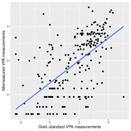
Figure 1: A scatter plot of the logarithm of the vigorous physical activity (VPA) measurements (METs$\cdot$h$\cdot$wk^-1) in the HPFS validation study, where the $x$-axis is the gold-standard measurements based on physical activity diaries and the $y$-axis is the error-prone measurements based on questionnaires. A linear regression line is added in blue color.

Our contributions to the literature are two-folded. First, in the typical scenario with a rare outcome and no exposure-mediator interaction, we derive new asymptotic bias expressions of the uncorrected estimators for all mediation effect measures under a Berkson-like measurement error model (Carroll et al., 2006). Second, we propose bias-correction strategies to permit valid estimation and inference for the mediation effect measures with an error-prone continuous exposure, allowing for exposure-mediator interactions and accommodating both common as well as rare outcomes. Our work differs from Zhao and Prentice (2014) in two distinct ways: (i) Zhao and Prentice (2014) assumes that parameters for characterizing the measurement error process are known or can be elicited from prior information. Relaxing that strong assumption, we leverage a validation study to estimate the measurement error process and account for the uncertainty in estimating the measurement error model parameters in inference about the mediation effect measures. (ii) Zhao and Prentice (2014) only considers mediation analysis with a rare outcome in the absence of exposure-mediator interaction in the outcome model, which can be restrictive in certain applications. Our work allows for exposure-mediator interactions and can be applied to either a rare or common outcome.

The paper is organized as follows. Section 2 reviews causal mediation analysis for a survival outcome without exposure measurement error. In Section 3, we describe the assumed measurement error model and derive explicit bias expressions for the uncorrected estimators of the mediation effect measures. The bias-correction methods are developed in Section 4 and 5, followed by a simulation study in Section 6 to evaluate their empirical performance. In Section 7, we apply the methods to the HPFS. Section 8 concludes.

2 Preliminaries on mediation analysis with a survival outcome

Let $A$ denote an exposure of interest, $M$ a mediator, $\widetilde{T}$ a time-to-event outcome, $\bm{W}$ a set of covariates. A diagram capturing the causal relationships among those variables is presented in Figure 2. In large prospective cohort studies like HPFS, $\widetilde{T}$ is right-censored due to loss to follow-up. Therefore, we only observe $(T,\delta)$, where $\delta=\mathbb{I}(T\leq C)$ is the failure indicator and $T=\widetilde{T}\wedge C\wedge t^{*}$ is the observed failure time, $C$ is the censoring time and $t^{*}$ is the maximum follow-up time. The observed data consists of $n_{1}$ copies of $\{T_{i},\delta_{i},M_{i},A_{i},\bm{W}_{i}\}$.

Figure 2: Mediation directed acyclic graph, where $\bm{W}$, $A$, $M$, $\widetilde{T}$ are the baseline covariates, the exposure, the mediator, the survival outcome, respectively. Here, the $A\rightarrow M\rightarrow\widetilde{T}$ pathway denotes the natural indirect and the $A\rightarrow\widetilde{T}$ pathway denotes the natural direct effect.

Under the counterfactual outcomes framework, several definitions for the mediation effect measures for a survival outcome have been proposed as functions of the survival function, hazard ratio, and mean survival times (Lange and Hansen, 2011; VanderWeele, 2011). Here we pursue the mediation effect measures on the log-hazard ratio scale as they are widely used in health science studies. To define the mediation effect measures, we let $M_{a}$ be the counterfactual mediator that would have been observed if the exposure $A$ has been set to level $a$. Similarly, let $\widetilde{T}_{am}$ be the counterfactual outcome that would be observed if $A$ and $M$ has been set to levels $a$ and $m$, respectively. Given these counterfactual variables, we can decompose the TE for contrasting $a^{*}$ to $a$ on the log-hazard ratio scale as

$$\underbrace{\log\{\lambda_{\widetilde{T}_{aM_{a}}}\!(t|\bm{w})\}\!-\!\log\{\lambda_{\widetilde{T}_{a^{*}M_{a^{*}}}}\!(t|\bm{w})\}}_{\text{TE}_{a,a^{*}|\bm{w}}(t)}$$

$$= \underbrace{\log\{\lambda_{\widetilde{T}_{aM_{a}}}(t|\bm{w})\}\!-\!\log\{\lambda_{\widetilde{T}_{aM_{a^{*}}}}(t|\bm{w})\}}_{\text{NIE}_{a,a^{*}|\bm{w}}(t)}+\underbrace{\log\{\lambda_{\widetilde{T}_{aM_{a^{*}}}}(t|\bm{w})\}\!-\!\log\{\lambda_{\widetilde{T}_{a^{*}M_{a^{*}}}}(t|\bm{w})\}}_{\text{NDE}_{a,a^{*}|\bm{w}}(t)},$$

where $\lambda_{\widetilde{T}_{aM_{a^{*}}}}(t|\bm{w})$ is the hazard of the counterfactual outcome $\widetilde{T}_{aM_{a^{*}}}$ conditional on the covariates $\bm{W}=\bm{w}$. The NIE measures that, at time $t$, the extent to which the log-hazard of the outcome would change if the mediator were to change from the level that would be observed under $a^{*}$ versus $a$ but the exposure is fixed at level $a$. The NDE measures how much the log-hazard of the outcome at time $t$ would change if the exposure is set to be level $a$ versus $a^{*}$ but the mediator is fixed at the value it would have take under exposure level $a^{*}$. Given the TE and NIE, the MP is defined as $\text{MP}_{a,a^{*}|\bm{w}}(t)=\text{NIE}_{a,a^{*}|\bm{w}}(t)/\text{TE}_{a,a^{*}|\bm{w}}(t)$. Notice that in the survival data context all of the mediation effect measures are functions of the follow-up time $t$. Our primary interest is to estimate $\tau_{a,a^{*}|\bm{w}}(t)$, where $\tau$ can be NIE, NDE, TE, or MP. We require the following assumptions to identify the causal mediation effect measures, including consistency, positivity, composition and a set of no unmeasured confounding assumptions; details of these assumptions are given in Web Appendix A. In addition, we assume the censoring time is conditionally independent from the survival time given covariates such that $C\perp\widetilde{T}|\{A,M,\bm{W}\}$.

To assess mediation, we consider the following semiparametric structural models for the mediator and outcome introduced in VanderWeele (2011) :

$$M=\alpha_{0}+\alpha_{1}A+\bm{\alpha}_{2}^{T}\bm{W}+\epsilon_{M},$$ (1)

$$\lambda_{\widetilde{T}}(t|A,M,\bm{W})=\lambda_{0}(t)e^{\beta_{1}A+\beta_{2}M+\beta_{3}AM+\bm{\beta}_{4}^{T}\bm{W}},$$ (2)

where $\epsilon_{M}\sim N(0,\sigma_{M}^{2})$, $\lambda_{\widetilde{T}}(t|A,M,\bm{W})$ is the hazard of the survival time conditional on levels of $[A,M,\bm{W}]$, $\lambda_{0}(t)$ is the unspecified baseline hazard, and $\beta_{3}$ is the exposure-mediator interaction on outcome. Let $\bm{\theta}=\left[\bm{\alpha}^{T},\bm{\beta}^{T}\right]^{T}$ be all the parameters in the mediator and outcome models, where $\bm{\alpha}=[\alpha_{0},\alpha_{1},\bm{\alpha}_{2}^{T},\sigma_{M}^{2}]^{T}$ and $\bm{\beta}=[\beta_{1},\beta_{2},\beta_{3},\bm{\beta}_{4}^{T}]^{T}$. From (1) and (2) and under the aforementioned identifiability assumptions, VanderWeele (2011) showed that

$$\text{NIE}_{a,a^{*}|\bm{w}}(t) =\delta_{a,a|\bm{w}}\left(\Lambda_{0}(t),\bm{\theta}\right)-\delta_{a,a^{*}|\bm{w}}\left(\Lambda_{0}(t),\bm{\theta}\right),$$ (3)

$$\text{NDE}_{a,a^{*}|\bm{w}}(t) =\delta_{a,a^{*}|\bm{w}}\left(\Lambda_{0}(t),\bm{\theta}\right)-\delta_{a^{*},a^{*}|\bm{w}}\left(\Lambda_{0}(t),\bm{\theta}\right),$$

where $\Lambda_{0}(t)=\int_{0}^{t}\lambda_{0}(u)du$ is the cumulative baseline hazard,

$$\delta_{a,a^{*}|\bm{w}}\left(\Lambda_{0}(t),\bm{\theta}\right)= \log\left\{r_{a,a^{*}|\bm{w}}(t)\right\}+(\beta_{1}a+\bm{\beta}_{4}^{T}\bm{w})+(\beta_{2}+\beta_{3}a)(\alpha_{0}+\alpha_{1}a^{*}+\bm{\alpha}_{2}^{T}\bm{w})$$

$$+0.5(\beta_{2}+\beta_{3}a)^{2}\sigma_{M}^{2},$$

and

$$r_{a,a^{*}|\bm{w}}(t)\!=\!\frac{\int_{m}\exp\left(\!-\!\Lambda_{0}(t)e^{(\beta_{2}+\beta_{3}a)^{2}+\beta_{1}a+\beta_{2}m+\beta_{3}am+\bm{\beta}_{4}^{T}\bm{w}}\right)\exp\left(-0.5(m\!-\!\alpha_{0}\!-\!\alpha_{1}a^{*}-\!\bm{\alpha}_{2}^{T}\bm{w})^{2}\right)dm}{\int_{m}\exp\left(-\Lambda_{0}(t)e^{\beta_{1}a+\beta_{2}m+\beta_{3}am+\bm{\beta}_{4}^{T}\bm{w}}\right)\exp\left(-0.5(m\!-\!\alpha_{0}\!-\!\alpha_{1}a^{*}\!-\!\bm{\alpha}_{2}^{T}\bm{w})^{2}\right)dm}.$$

Expressions for the $\text{TE}_{a,a^{*}|\bm{w}}(t)$ and $\text{MP}_{a,a^{*}|\bm{w}}(t)$ can be obtained by summing the NIE and NDE expressions and taking the ratio of the NIE and TE expressions, respectively. Therefore, once estimates of $\bm{\theta}$ and $\Lambda_{0}(t)$ are obtained, one can substitute them into (3) to obtain the estimates for mediation effect measures.

While the exact expressions (3) is appealing to calculate the mediation effect measures, it can be computationally complex because the expressions involve integrals that typically do not have a closed-form solution. In health science studies, the survival outcome is oftentimes rare (for example, the cumulative event rate is below 10%, or $\Lambda_{0}(t)\approx 0$), in which case the mediation effect measure expressions can be substantially simplified (VanderWeele, 2011). Specifically, because $r_{a,a^{*}|\bm{w}}(t)\approx 1$ when $\Lambda_{0}(t)\approx 0$, we arrive at the following approximate expressions:

$$\text{NIE}_{a,a^{*}|\bm{w}}(t) \approx(\beta_{2}\alpha_{1}+\beta_{3}\alpha_{1}a)(a-a^{*}),$$

$$\text{NDE}_{a,a^{*}|\bm{w}}(t) \approx\left\{\beta_{1}+\beta_{3}(\alpha_{0}+\alpha_{1}a^{*}+\bm{\alpha}_{2}^{T}\bm{w}+\beta_{2}\sigma_{M}^{2})\right\}(a-a^{*})+0.5\beta_{3}^{2}\sigma_{M}^{2}(a^{2}-{a^{*}}^{2}).$$

which are free of the baseline hazard and therefore are constant over time. Approximate expressions of TE and MP can be obtained accordingly. If we further assume no mediator-exposure interaction in the Cox model ($\beta_{3}=0$), we obtain $\text{NIE}_{a,a^{*}|\bm{w}}(t)\approx\beta_{2}\alpha_{1}(a-a^{*})$ and $\text{NDE}_{a,a^{*}|\bm{w}}(t)\approx\beta_{1}(a-a^{*})$. In what follows, we primarily discuss the mediation effect measures based upon the approximate expressions under a rare outcome assumption. Since the approximate mediation effect measures are constant over $t$, we shall rewrite $\tau_{a,a^{*}|\bm{w}}(t)$ to $\tau_{a,a^{*}|\bm{w}}$ without ambiguity. Extensions to a common outcome are provided in Section 5.

3 Implications of exposure measurement error on assessing mediation

The exposure variable variable in health science research is usually measured with error due to technology or budget limitations. In the HPFS, vigorous physical activity (the exposure of interest in our application study) was assessed through self-administrative questionnaires. While it is known to be error-prone, using self-administrative questionnaires is a more cost-effective and practical option, comparing to the gold-standard measurement of physical activity through diaries. In the presence of exposure measurement error, only a mismeasured version of exposure, $A^{*}$, is available so that we only observe $\{T_{i},\delta_{i},M_{i},A_{i}^{*},\bm{W}_{i}\}$, $i=1,\dots,n_{1}$. We denote this data sample as the main study to distinguish it from the validation study that will be introduced later. We assume the relationship between $A$ and $A^{*}$ can be characterized by the following Berkson-like measurement error model (Carroll et al., 2006; Rosner et al., 1990):

$$A=\gamma_{0}+\gamma_{1}A^{*}+\bm{\gamma}_{2}^{T}\bm{W}+\epsilon_{A},$$ (4)

where $\epsilon_{A}$ is a mean-zero error term with a constant variance $\sigma_{A}^{2}$. We call $\gamma_{1}$ the calibration coefficient that represents the association between $A$ and $A^{*}$ conditional on $\bm{W}$. Throughout, we employ the standard surrogacy assumption to ensure that $P(\widetilde{T}|A,A^{*},M,\bm{W})=P(\widetilde{T}|A,M,\bm{W})$ and $P(M|A,A^{*},\bm{W})=P(M|A,\bm{W})$ such that the error-prone measurement $A^{*}$ is not informative for the outcome and mediator given the true exposure $A$.

If the true exposure $A$ is replaced by the error-prone exposure $A^{*}$ in models (1) and (2), then estimators of the regression parameters $\bm{\theta}$ may be biased; and hence estimates for the mediation effect measures will also be subject to bias. Let $\widehat{\tau}_{a,a^{*}|\bm{w}}^{*}$ be the uncorrected estimator of $\tau_{a,a^{*}|\bm{w}}$ when $A$ is not available in models (1) and (2) and $A^{*}$ is used instead. The following result presents the bias of the uncorrected estimators under the rare outcome scenario and in the absence of exposure-mediator interaction ($\beta_{3}=0$ in model (2)).

Theorem 1

Define $RelBias(\widehat{\tau}_{a,a^{*}|\bm{w}}^{*})=\underset{n\rightarrow\infty}{\text{lim}}(\widehat{\tau}_{a,a^{*}|\bm{w}}^{*}-\tau_{a,a^{*}|\bm{w}})/{\tau_{a,a^{*}|\bm{w}}}$ as the relative bias of the uncorrected estimator $\widehat{\tau}_{a,a^{*}|\bm{w}}^{*}$ and

$$\rho={\sigma_{A}^{2}}/(\sigma_{A}^{2}+\sigma_{M}^{2}/\alpha_{1}^{2}).$$

Suppose the outcome is rare and $\beta_{3}=0$ in model (2). Then, if the error term in model (4) is normally distributed such that $\epsilon_{A}\sim N(0,\sigma_{A}^{2})$, the asymptotic relative bias for each uncorrected estimator of the mediation effect measures are given by

$$RelBias(\widehat{\text{NIE}}_{a,a^{*}|\bm{w}}^{*}) \approx\gamma_{1}-1+\gamma_{1}\rho\left({1}/{\text{MP}_{a,a^{*}|\bm{w}}}-1\right)$$

$$RelBias(\widehat{\text{NDE}}_{a,a^{*}|\bm{w}}^{*}) \approx(\gamma_{1}-1)(1-\rho)-\rho,$$

$$RelBias(\widehat{\text{TE}}_{a,a^{*}|\bm{w}}^{*}) \approx\gamma_{1}-1$$

$$RelBias(\widehat{\text{MP}}_{a,a^{*}|\bm{w}}^{*}) \approx\rho\left({1}/{\text{MP}_{a,a^{*}|\bm{w}}}-1\right).$$

The proof of Theorem 1 is presented in Web Appendix B. Theorem 1 indicates that, as long as the outcome is rare with no exposure-mediator interaction, the relative bias of the uncorrected estimators only depends on two parameters, $\gamma_{1}$ and $\rho$, where $\gamma_{1}$ is the calibration coefficient and $\rho$, as is defined in Theorem 1, is a proportion that takes values from 0 to 1. In this paper, we name $\rho$ the MP reliability index as it fully determine the relative bias of the uncorrected estimator of MP as suggested in Theorem 1. Evidently, all uncorrected estimators will be unbiased when $\gamma_{1}=1$ and $\rho=0$, otherwise the uncorrected estimators tend to have a specific direction of bias. Specifically, the NIE estimator will be biased away or toward the null when $\gamma_{1}$ is larger or smaller than

$${1}\Big{/}\left(1+\rho(1/\text{MP}_{a,a^{*}|\bm{w}}^{*}-1)\right),$$

respectively. The NDE estimator will only have a positive relative bias when $\gamma_{1}>1/(1-\rho)$. The direction of relative bias of the TE estimator only depends on $\gamma_{1}$, with $\gamma_{1}>1$ and $<1$ corresponding to a positive and negative bias, respectively. The MP estimator will always have a positive relative bias since $\rho\geq 0$, suggesting the uncorrected estimator will always exaggerate the true MP.

Below we give the intuition on the MP reliability index, $\rho$, under the scenario with no covariates. Let $\rho_{AA^{*}}=\text{Corr}(A,A^{*})$ and $\rho_{AM}=\text{Corr}(A,M)$ be the correlation coefficients between $A$ and $A^{*}$ and between $A$ and $M$, respectively. When $\bm{W}=\emptyset$, Web Appendix B.2 shows that

$$\rho=\frac{1-\rho_{AA^{*}}^{2}}{1/\rho_{AM}^{2}-\rho_{AA^{*}}^{2}},$$

which is bounded within $\rho\in[0,\rho_{AM}^{2}]$ regardless of the value of $\rho_{AA^{*}}$. Therefore, $\rho$ will be close to 0 if either the exposure measurement error is small (i.e., $|\rho_{AA^{*}}|$ is large) or the exposure-mediator association is weak (i.e., $\rho_{AM}$ is small). Under either condition, the uncorrected NIE, NDE, and TE estimators will share the same asymptotic relative bias, $\gamma_{1}-1$, and the MP estimator will be approximately unbiased as $\rho\approx 0$. Figure 3 provides a visualization on the value of $\rho$ in terms of $\rho_{AA^{*}}$ and $\rho_{AM}$, and indicates that $\rho$ is below 0.1 when either (i) $\rho_{AM}\leq 0.3$ or (ii) $\rho_{AM}\leq 0.4$ and $\rho_{AA^{*}}\geq 0.65$. Therefore, the uncorrected MP estimator usually presents relatively small biases, because it is relatively uncommon to simultaneously find a strong exposure-mediator association alongside a medium to large exposure measurement error.

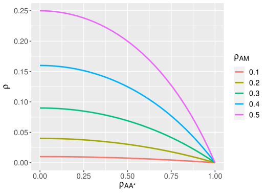
Figure 3: A visualization of the MP reliability index ($\rho$) in terms of the correlation coefficient between exposure and mediator ($\rho_{AM}$) and the correlation coefficient between the exposure and its mismeasured surrogate ($\rho_{AA^{*}}$).

In Web Appendix B.3, we present an interesting observation that all bias formulas in Theorem 1 coincide with the exposure measurement error-induced bias in mediation analysis with a binary outcome in Cheng et al. (2023), although the mediation effect measures are defined differently and also assessed by different approaches. Specifically, the present work defines the mediation effect measures at a log-hazard ratio scale and considers using one outcome model and one mediator model for purpose of estimation. The mediation effect measures in Cheng et al. (2023) are defined at a log-risk ratio scale and are estimated using the difference method with two log-binomial regression models on the outcome. Although the settings between these two work are different, their bias formulas happen to be identical.

Theorem 1 is derived under the assumption with a rare outcome with no exposure-mediator interaction. In the presence of an exposure-mediator interaction, the bias will have a more complex form and dependent on all of regression parameters $\bm{\theta}$, and thus analytically intractable. Next, we develop bias correction approaches to ensure valid estimation for mediation effect measures with a mismeasured exposure, in more general settings that permit an exposure-mediator interaction and even a common outcome.

4 Correcting for exposure measurement error-induced bias

We now propose methods to correct for the exposure measurement error in estimating mediation effect measures. In addition to the main study, $\{T_{i},\delta_{i},M_{i},A_{i}^{*},\bm{W}_{i}\}$, $i=1,\dots,n_{1}$, we require a validation study to identify the parameters in the measurement error model (4). As is suggested by our application study, we assume the true exposure measurements are available among the validation study participants. Specifically, the validation study consists of data $\{T_{i},M_{i},A_{i}^{*},A_{i},\bm{W}_{i}\}$, $i=n_{1}+1,\dots,n$. We consider an external validation study where failure indicator $\delta_{i}$ is not available (Liao et al., 2011). To ensure that the parameters estimated in the validation study can be validly transported to the main study, we require the transportability assumption such that the joint distribution of $P(A,M,T,C|A^{*},\bm{W})$ in the validation study is identical to its counterpart in the main study (Yi et al., 2015). The transportability assumption is plausible in our application analysis, because (i) both the main and validition study in the HPFS share the same way for assessing the mismeasured version of exposure $A^{*}$ through self-adminstrated questionnaires and (ii) study participants in the validation study are draw from the same target population with the HPFS main study.

The parameters in the measurement error model (4), $\bm{\gamma}=[\gamma_{0},\gamma_{1},\bm{\gamma}_{2},\sigma_{A}^{2}]$, can be estimated by regressing $A$ on $\{A^{*},\bm{W}\}$ in the validation study; i.e., $\widehat{\bm{\gamma}}$ solves

$$\sum_{i=1}^{n}(1-R_{i})\left\{\begin{matrix}(1,A_{i}^{*},\bm{W}_{i}^{T})^{T}(A_{i}-\gamma_{0}-\gamma_{1}A_{i}^{*}-\bm{\gamma}_{2}^{T}\bm{W}_{i})\\ \sigma_{A}^{2}-(A_{i}-\gamma_{0}-\gamma_{1}A_{i}^{*}-\bm{\gamma}_{2}^{T}\bm{W}_{i})^{2}\end{matrix}\right\}=\bm{0},$$ (5)

where $R_{i}$ is an indicator with $R_{i}=0$ if the individual is in the validation study (i.e., $i>n_{1}$) and $R_{i}=1$ if the individual is in the main study (i.e., $i\leq n_{1}$). One can verify that $[\widehat{\gamma}_{0},\widehat{\gamma}_{1},\widehat{\bm{\gamma}}_{2}]$ is the ordinary least squares (OLS) estimator of the regression coefficients in model (4) and $\widehat{\sigma}_{A}^{2}$ is the empirical variance of the residuals of model (4) in the validation study. Notice that $\widehat{\bm{\gamma}}$ is consistent if (4) is correctly specified, regardless of whether $\epsilon_{A}$ is normally distributed. In what follows, we discuss estimation of parameters in the mediator and outcome models, separately.

4.1 Estimation of the mediator model parameters

The mediator model (1) involves variables $\{M_{i},A_{i},\bm{W}_{i}\}$, which are fully observed in the validation study. A convenient approach for estimating $\bm{\alpha}$ is to regress $M$ on $A$ and $\bm{W}$ in the validation study alone but this dispenses with any information from the main study. Below we pursue an approach to estimate the mediator model that efficiently uses the information from both studies. Combining the measurement error model (4) and mediator model (1), we can show the first two moments of the mediator given the mismeasured exposure and covariates are $E[M|A^{*},\bm{W}]=\alpha_{0}+\alpha_{1}\mu_{A}(\bm{\gamma})+\bm{\alpha}_{2}^{T}\bm{W}$ and $\text{Var}(M|A^{*},\bm{W})=\sigma_{M}^{2}+\alpha_{1}^{2}\sigma_{A}^{2}$, where $\mu_{A}(\bm{\gamma})=\gamma_{0}+\gamma_{1}A^{*}+\bm{\gamma}_{2}^{T}\bm{W}$ is the conditional mean of the $A|A^{*},\bm{W}$ implied by model (4). Comparing $E[M|A^{*},\bm{W}]$ to $E[M|A,\bm{W}]$ in (1), one can observe that fitting (1) with $A$ replaced by $\mu_{A}(\bm{\gamma})$ leads to valid estimates of the regression coeffcients in the mediator model, $[\alpha_{0},\alpha_{1},\bm{\alpha}_{2}^{T}]$. This suggests the following estimating equations for $[\alpha_{0},\alpha_{1},\bm{\alpha}_{2}^{T}]$:

$$\sum_{i=1}^{n}R_{i}\left(1,\mu_{A_{i}}(\widehat{\bm{\gamma}}),\bm{W}_{i}^{T}\right)^{T}(M_{i}\!-\!\alpha_{0}\!-\!\alpha_{1}\mu_{A_{i}}(\widehat{\bm{\gamma}})\!-\!\bm{\alpha}_{2}^{T}\bm{W}_{i})$$

$$\quad\quad+(1-R_{i})\left(1,A_{i},\bm{W}_{i}^{T}\right)^{T}(M_{i}\!-\!\alpha_{0}\!-\!\alpha_{1}A_{i}\!-\!\bm{\alpha}_{2}^{T}\bm{W}_{i})=\bm{0}$$ (6)

where $\mu_{A_{i}}(\widehat{\bm{\gamma}})=\widehat{\gamma}_{0}+\widehat{\gamma}_{1}A^{*}+\widehat{\bm{\gamma}}_{2}^{T}\bm{W}$ is obtained by fitting model (4) in the validation study. The estimating equation (6) utilizes data from both the main and the validation studies. Specifically, for observations in the validation study ($R_{i}=0$), equation (6) uses the true likelihood score for $[\alpha_{0},\alpha_{1},\bm{\alpha}_{2}^{T}]$; for observations in the main study ($R_{i}=1$), equation (6) uses a pseudo likelihood score that replaces $A_{i}$ in the original likelihood score by its predicted value $\mu_{A_{i}}(\widehat{\bm{\gamma}})$ based on the measurement error model fit.

Similarly to (6), we can construct the following estimating equation for $\sigma_{M}^{2}$:

$$\sum_{i=1}^{n}R_{i}\Big{(}\sigma_{M}^{2}+\widehat{\alpha}_{1}^{2}\widehat{\sigma}_{A}^{2}-(M_{i}-\widehat{\alpha}_{0}-\widehat{\alpha}_{1}\mu_{A}(\widehat{\bm{\gamma}})-\widehat{\bm{\alpha}}_{2}^{T}\bm{W}_{i})^{2}\Big{)}$$

$$\quad\quad\quad+(1-R_{i})\Big{(}\sigma_{M}^{2}-(M_{i}-\widehat{\alpha}_{0}-\widehat{\alpha}_{1}A_{i}-\widehat{\bm{\alpha}}_{2}^{T}\bm{W}_{i})^{2}\Big{)}=0,$$ (7)

where $[\widehat{\alpha}_{0},\widehat{\alpha}_{1},\widehat{\bm{\alpha}}_{2}^{T}]$ is obtained by (6). Equation (7) has a explicit solution such that

$$\widehat{\sigma}_{M}^{2}=\frac{1}{n}\sum_{i=1}^{n}\left[M_{i}-\widehat{\alpha}_{0}-\widehat{\alpha}_{1}\Big{(}R_{i}\mu_{A}(\widehat{\bm{\gamma}})+(1-R_{i})A_{i}\Big{)}-\widehat{\bm{\alpha}}_{2}^{T}\bm{W}_{i}\right]^{2}-\frac{n_{1}}{n}\widehat{\alpha}_{1}^{2}\widehat{\sigma}_{A}^{2}.$$

4.2 Estimation of the outcome model parameters via ORC

Given the true hazard function (2), the induced hazard function of $\widetilde{T}$ given the mismeasured exposure $A^{*}$ instead of $A$ is

$$\lambda_{\widetilde{T}}(t|A^{*},M,\bm{W}) =\lambda_{0}(t)e^{\beta_{2}M+\bm{\beta}_{4}^{T}\bm{W}}E[e^{(\beta_{1}+\beta_{3}M)A}|A^{*},M,\bm{W},T\geq t].$$ (8)

From (8), we see the critical quantity is $E[e^{(\beta_{1}+\beta_{3}M)A}|A^{*},M,\bm{W},T\geq t]$, which does not have an explicit expression. The ordinary regression calibration (ORC) approach uses the rare outcome assumption to approximate the critical quantity. Prentice (1982) shows that $E[e^{(\beta_{1}+\beta_{3}M)A}|A^{*},M,\bm{W},T\geq t]\approx E[e^{(\beta_{1}+\beta_{3}M)A}|A^{*},M,\bm{W}]$ if the the outcome is rare. Then, we can further use a first-order Taylor expansion to approximate $E[e^{(\beta_{1}+\beta_{3}M)A}|A^{*},M,\bm{W}]$ by $e^{(\beta_{1}+\beta_{3}M)E[A|A^{*},M,\bm{W}]}$. The Taylor approximation is exact when $A|\{A^{*},M,\bm{W}\}$ is normally distributed with a constant variance and in the absence of any exposure-mediator interaction. Otherwise, the approximation is valid when either (i) $A|\{A^{*},M,\bm{W}\}$ is normal and $(\beta_{1}+\beta_{3}M)^{2}\text{Var}(A|A^{*},M,\bm{W})$ is small, or (ii) $|\beta_{1}|+|\beta_{3}|$ and $(\beta_{1}+\beta_{3}M)^{2}\text{Var}(A|A^{*},M,\bm{W})$ are small, or (iii) $|\beta_{1}|$ is small with no exposure-mediator interaction and $\text{Var}(A|A^{*},M,\bm{W})=\sigma^{2}$ is constant (see Web Appendix C.1 for detail discussion about the approximation). Based on this approximation, we can rewrite the induced hazard (8) as the following Cox model

$$\lambda_{\widetilde{T}}(t|A^{*},M,\bm{W})\approx\lambda_{0}(t)e^{\beta_{1}E[A|A^{*},M,\bm{W}]+\beta_{2}M+\beta_{3}ME[A|A^{*},M,\bm{W}]+\bm{\beta}_{4}^{T}\bm{W}}.$$ (9)

This indicates that, with an appropriate estimator $\widehat{E}[A|A^{*},M,\bm{W}]$, we can obtain $\widehat{\bm{\beta}}$ by simply implementing Cox model (2) based on the main study with $A$ imputed by $\widehat{E}[A|A^{*},M,\bm{W}]$.

We provide two strategies to calculate $\widehat{E}[A|A^{*},M,\bm{W}]$. First, observing that all of the variables used in $E[A|A^{*},M,\bm{W}]$ are fully observed in the validation study, one can specify a model for $E[A|A^{*},M,\bm{W}]$ based on the validation study directly. For example, we can first specify the following regression for $E[A|A^{*},M,\bm{W}]$:

$$E[A|A^{*},M,\bm{W}]=\eta_{0}+\eta_{1}A^{*}+\eta_{2}M+\bm{\eta}_{3}^{T}\bm{W},$$ (10)

with coefficients $\bm{\eta}=[\eta_{0},\eta_{1},\eta_{2},\bm{\eta}_{3}]$. Next, we calculate the OLS estimator, $\widehat{\bm{\eta}}$, by solving

$$\sum_{i=1}^{n}(1-R_{i})\left(1,A_{i}^{*},M_{i},\bm{W}_{i}^{T}\right)^{T}\left(A_{i}-\eta_{0}-\eta_{1}A_{i}^{*}-\eta_{2}M_{i}-\bm{\eta}_{3}^{T}\bm{W}_{i}\right)=\bm{0},$$ (11)

and then obtain $\widehat{E}[A|A^{*},\bm{M},\bm{W}]=m_{A}^{(O1)}(\widehat{\bm{\eta}})$, where $m_{A}^{(O1)}(\widehat{\bm{\eta}})=\widehat{\eta}_{0}+\widehat{\eta}_{1}A^{*}+\widehat{\eta}_{2}M+\widehat{\bm{\eta}}_{3}^{T}\bm{W}$ is the estimated conditional mean of (10). An alternative approach to calculate $\widehat{E}[A|A^{*},\bm{M},\bm{W}]$ is deriving its analytic form based on the measurement error model (4) and the mediator model (1). This approach requires the distributional assumption of the error term in model (4), $\epsilon_{A}$. If $\epsilon_{A}$ is normally distributed, we show that $E[A|A^{*},M,\bm{W}]=m_{A}^{(O2)}({\bm{\alpha}},{\bm{\eta}})$, where

$$m_{A}^{(O2)}({\bm{\alpha}},{\bm{\gamma}})=\frac{\gamma_{0}\sigma_{M}^{2}-\alpha_{0}\alpha_{1}\sigma_{A}^{2}}{\alpha_{1}^{2}\sigma_{A}^{2}+\sigma_{M}^{2}}+\frac{\gamma_{1}\sigma_{M}^{2}}{\alpha_{1}^{2}\sigma_{A}^{2}+\sigma_{M}^{2}}A^{*}+\frac{\alpha_{1}\sigma_{A}^{2}}{\alpha_{1}^{2}\sigma_{A}^{2}+\sigma_{M}^{2}}M+\frac{\sigma_{M}^{2}\bm{\gamma}_{2}^{T}-\alpha_{1}\sigma_{A}^{2}\bm{\alpha}_{2}^{T}}{\alpha_{1}^{2}\sigma_{A}^{2}+\sigma_{M}^{2}}\bm{W}$$ (12)

by applying the Bayes formula on (4) and (1) (See Lemma 1 in the Supplementary Material for the proof). Therefore, the second strategy is to obtain $\widehat{E}[A|A^{*},\bm{M},\bm{W}]=m_{A}^{(O2)}(\widehat{\bm{\alpha}},\widehat{\bm{\gamma}})$ by replacing $(\bm{\alpha},\bm{\gamma})$ in (12) with their corresponding point estimators.

Denote $\widehat{\bm{\beta}}^{(O1)}$ and $\widehat{\bm{\beta}}^{(O2)}$ as the ORC estimators of $\bm{\beta}$ by using the strategies (10) and (12), respectively. Comparing both estimators, $\widehat{\bm{\beta}}^{(O1)}$ requires fitting an additional model for $E[A|A^{*},\bm{M},\bm{W}]$, whereas $\widehat{\bm{\beta}}^{(O2)}$ more effectively use the information from the measurement error model and mediator model to derive an analytic form of $E[A|A^{*},\bm{M},\bm{W}]$. Validity of $\widehat{\bm{\beta}}^{(O2)}$ depends on a correctly specified measurement error model (4) with a normal error term, where $\widehat{\bm{\beta}}^{(O1)}$ only requires that the model (10) is correctly specified.

4.3 Estimation of the outcome model parameters via RRC

Performance of the ORC may be compromised under departure from the rare outcome assumption. Following Xie et al. (2001) and Liao et al. (2011), we further consider a risk set calibration (RRC) approach to estimate $\bm{\beta}$, which uses a closer approximation to the induced hazard (8) without the rare outcome assumption. Specifically, we propose to use a first order Taylor expansion to approximate the critical quantity $E[e^{(\beta_{1}+\beta_{3}M)A}|A^{*},M,\bm{W},T\geq t]$ by $e^{(\beta_{1}+\beta_{3}M)E[A|A^{*},M,\bm{W},T\geq t]}$ and then the induced hazard (8) becomes

$$\lambda_{\widetilde{T}}(t|A^{*},M,\bm{W})\approx\lambda_{0}(t)e^{\beta_{1}E[A|A^{*},M,\bm{W},T\geq t]+\beta_{2}M+\beta_{3}ME[A|A^{*},M,\bm{W},T\geq t]+\bm{\beta}_{4}^{T}\bm{W}},$$ (13)

where the approximation is exact when $A|\{A^{*},M,\bm{W},T\geq t\}$ is normal, the variance $\text{Var}(A|A^{*},M,\bm{W},T\geq t)$ is only a function of $t$, and there is no exposure-mediator interaction ($\beta_{3}=0$). The approximation is also valid when (i) $A|\{A^{*},M,\bm{W},T\geq t\}$ is normal and $(\beta_{1}+\beta_{3}M)^{2}\text{Var}(A|A^{*},M,\bm{W},T\geq t)$ is small, or (ii) $|\beta_{1}|+|\beta_{3}|$ and $(\beta_{1}+\beta_{3}M)^{2}\text{Var}(A|A^{*},M,\bm{W},T\geq t)$ are small, or (iii) $|\beta_{1}|$ is small with no exposure-mediator interaction and $\text{Var}(A|A^{*},M,\bm{W},T\geq t)$ only depends on $t$ (see Web Appendix C.2 for detail discussion of the approximations). We propose the following regression model for $E[A|A^{*},M,\bm{W},T\geq t]$:

$$E[A|A^{*},M,\bm{W},T\geq t]=\xi_{0}(t)+\xi_{1}(t)A^{*}+\xi_{2}(t)M+\bm{\xi}_{3}^{T}(t)\bm{W},$$ (14)

where $\bm{\xi}(t)=[\xi_{0}(t),\xi_{1}(t),\xi_{2}(t),\bm{\xi}_{0}^{T}(t)]^{T}$ are time-dependent coefficients. The basic idea underlying the RRC is re-estimating model (14) from the validation study at each main study failure time and then running the Cox model (2) among the main study samples with $A_{i}$ estimated as its predicted value from (14). However, this may be computationally burdensome when the number of unique failure time is large. More importantly, because precise measurement of the exposure is often expensive in health sciences research, the validation study is usually small to accurately estimate model (14) at each main study failure time. For example, the HPFS validation study in our applications involves a total of 238 participants, which is disproportionately small comparing to the main study sample size ($n_{1}=43,573$). Observing the small validation study sample size in our application study, we propose to group the risk sets to stabilize the results and facilitate computation, with a similar spirit to Zhao and Prentice (2014) and Liao et al. (2018).

The proposed RRC estimation procedure is as follows: Step 1, divide the main study follow-up duration $[0,t^{*}]$ in to $K$ intervals, $[t_{1},t_{2})$, $[t_{2},t_{3})$, $\dots$, $[t_{K},t^{*}]$, where $t_{1}=0$. Step 2, find the $K$ risk sets in the validation study, $R_{v}(t_{k})$, $k=1,\dots,K$, such that $R_{v}(t_{k})$ includes all individuals with $(1\!-\!R_{i})Y_{i}(t_{k})=1$, where $Y_{i}(t)=\mathbb{I}(T_{i}\geq t)$ is the risk process indicator. Step 3, for each $t_{k}$, obtain $\widehat{\bm{\xi}}(t_{k})$ by regressing $A$ on $(A^{*},M,\bm{W})$ among individuals in the risk set $R_{v}(t_{k})$; i.e., obtain $\widehat{\bm{\xi}}(t_{k})$ by solving

$$\sum_{i=1}^{n}(1\!-\!R_{i})Y_{i}(t_{k})\left(1,A_{i}^{*},M_{i},\bm{W}_{i}^{T}\right)^{T}\Big{(}A_{i}-\xi_{0}(t_{k})-\xi_{1}(t_{k})A_{i}^{*}-\xi_{2}(t_{k})M_{i}-\bm{\xi}_{3}^{T}(t_{k})\bm{W}_{i}\Big{)}=\bm{0}.$$ (15)

Step 4, let $m_{A_{i}}^{(R)}(\widehat{\bm{\xi}})=\widehat{\xi}_{0}(T_{i}^{*})+\widehat{\xi}_{1}(T_{i}^{*})A_{i}^{*}+\widehat{\xi}_{2}(T_{i}^{*})M_{i}+\widehat{\bm{\xi}}_{3}^{T}(T_{i}^{*})\bm{W}_{i}$, where $T_{i}^{*}$ is the most recent available $t_{k}$ that is at or prior to $T_{i}$. Step 5, finally, run the Cox model (2) in the main study with $A_{i}$ in replacement by $m_{A_{i}}^{(R)}(\widehat{\bm{\xi}})$ to get the point estimator of $\bm{\beta}$, denoted by $\widehat{\bm{\beta}}^{(R)}$.

The choice of the split points $t_{k}$, $k=1,\dots,K$, can be flexible. For example, following Zhao and Prentice (2014), one can equally divide the time scale into $K$ intervals such that $t_{k}=\frac{(k-1)t_{v}^{*}}{K}$, where $t_{v}^{*}$ is the maximum observed failure time in the validation study. Notice that $\widehat{\bm{\beta}}^{(R)}$ coincides with $\widehat{\bm{\beta}}^{(O1)}$ for $K=1$ since there are no split points between $[0,t^{*}]$. Performance of RRC with different number of $K$ is evaluated in Section 6. To determine the optimal number of risk sets ($K$), one can consider a range of candidate values of $K$, e.g., $K\in\{1,\dots,10\}$, and then use a cross-validation approach in the validation study samples to select the one with smallest mean-squared error or mean absolute error.

4.4 Asymptotic properties and variance estimation

We have proposed one estimator for the mediator model, $\widehat{\bm{\alpha}}$, and three estimators for the Cox outcome model, the ORC1 ($\widehat{\bm{\beta}}^{(O1)}$), the ORC2 ($\widehat{\bm{\beta}}^{(O2)}$), and the RRC ($\widehat{\bm{\beta}}^{(R)}$). These three estimators of $\bm{\beta}$ are the solution of the following score equation induced from model (2), but with different choice of $m_{A_{i}}$:

$$\sum_{i=1}^{n}R_{i}\int_{0}^{t^{*}}\left\{\bm{Z}_{i}-\frac{\sum_{i=1}^{n_{1}}Y_{i}(t)\exp\{\bm{\beta}^{T}\bm{Z}_{i}\}\bm{Z}_{i}}{\sum_{i=1}^{n_{1}}Y_{i}(t)\exp\{\bm{\beta}^{T}\bm{Z}_{i}\}}\right\}dN_{i}(t)=\bm{0},$$ (16)

where $\bm{Z}_{i}=\left[m_{A_{i}},M_{i},m_{A_{i}}M_{i},\bm{W}_{i}^{T}\right]^{T}$, $N_{i}(t)=\mathbb{I}(T_{i}\leq t,\delta_{i}=1)$ is the counting process, and $Y_{i}(t)=\mathbb{I}(T_{i}\geq t)$ is the risk process. Here, $m_{A_{i}}$ is the estimated value of $A_{i}$, which is set as $m_{A_{i}}^{(O1)}(\widehat{\bm{\eta}})$, $m_{A_{i}}^{(O2)}(\widehat{\bm{\alpha}},\widehat{\bm{\gamma}})$, and $m_{A_{i}}^{(R)}(\widehat{\bm{\xi}})$ by the ORC1, ORC2, and RRC methods, respectively. To summarize, we have three estimators for $\bm{\theta}$ characterized by their outcome model estimation approach, the ORC1, $\widehat{\bm{\theta}}^{(O1)}=\left[\widehat{\bm{\alpha}}^{T},\widehat{\bm{\beta}}^{(O1)^{T}}\right]^{T}$, the ORC2, $\widehat{\bm{\theta}}^{(O2)}=\left[\widehat{\bm{\alpha}}^{T},\widehat{\bm{\beta}}^{(O2)^{T}}\right]^{T}$, and the RRC, $\widehat{\bm{\theta}}^{(R)}=\left[\widehat{\bm{\alpha}}^{T},\widehat{\bm{\beta}}^{(R)^{T}}\right]^{T}$.

Theorem 2 states that $\widehat{\bm{\theta}}^{(O1)}$ is approximately consistent and asymptotically normal, where the proof is given in Web Appendix D:

Theorem 2

Under regularity conditions in Web Appendix D.1, $\widehat{\bm{\theta}}^{(O1)}\overset{p}{\to}\bm{\theta}_{0}^{(O1)}$, where $\bm{\theta}_{0}^{(O1)}=\left[\bm{\alpha}_{0}^{T},{\bm{\beta}_{0}^{(O1)}}^{T}\right]^{T}$, $\bm{\alpha}_{0}$ is the true value of $\bm{\alpha}$ in the mediator model (1), and $\bm{\beta}_{0}^{(O1)}$ is the true value of $\bm{\beta}$ in the approximate hazard model (9) with $E[A|A^{*},M,\bm{W}]$ defined in (10). In addition, we have $\sqrt{n}\left(\widehat{\bm{\theta}}^{(O1)}-\bm{\theta}_{0}^{(O1)}\right)\overset{D}{\to}N\left(\bm{0},\bm{V}^{(O1)}\right)$, where $\bm{V}^{(O1)}$ is provided in Web Appendix D.2.

This result shows that $\widehat{\bm{\alpha}}$ converges to the true value of $\bm{\alpha}$ but $\widehat{\bm{\beta}}^{(O1)}$ converges to $\bm{\beta}_{0}^{(O1)}$ that is close to but generally different from $\bm{\beta}$ in the true Cox model (2). Also, Theorem 2 suggests the following sandwich variance estimator of $\bm{V}^{(O1)}$:

$$\widehat{\bm{V}}^{(O1)}=\left[\widehat{\bm{I}}_{\bm{\theta}}^{(O1)}\right]^{-1}\widehat{\bm{M}}_{\bm{\theta}}^{(O1)}\left[\widehat{\bm{I}}_{\bm{\theta}}^{(O1)}\right]^{-T},$$

where $\widehat{\bm{M}}_{\bm{\theta}}^{(O1)}\!=\!\frac{1}{n}\displaystyle\sum_{i=1}^{n}\left\{\mathbb{U}_{\bm{\theta},i}^{(O1)}(\widehat{\bm{\theta}}^{(O1)},\widehat{\bm{\gamma}},\widehat{\bm{\eta}})-\widehat{\bm{I}}_{\bm{\theta},\bm{\gamma}}^{(O1)}\widehat{\bm{I}}_{\bm{\gamma}}^{-1}\mathbb{U}_{\bm{\gamma},i}(\widehat{\bm{\gamma}})-\widehat{\bm{I}}_{\bm{\theta},\bm{\eta}}^{(O1)}\widehat{\bm{I}}_{\bm{\eta}}^{-1}\mathbb{U}_{\bm{\eta},i}(\widehat{\bm{\eta}})\right\}^{\otimes 2}$ and $\widehat{\bm{I}}_{\bm{\theta}}^{(O1)}=\frac{1}{n}\frac{\partial}{\partial\bm{\theta}}\mathbb{U}_{\bm{\theta}}^{(O1)}(\widehat{\bm{\theta}}^{(O1)},\widehat{\bm{\gamma}},\widehat{\bm{\eta}})$ and $\bm{v}^{\otimes 2}=\bm{v}\bm{v}^{T}$ for a vector $\bm{v}$. Here, we use $\mathbb{U}_{\bm{\omega}}(\bm{\omega},\bm{\omega}^{*})$ and $\mathbb{U}_{\bm{\omega},i}(\bm{\omega},\bm{\omega}^{*})$ to denote the estimating equation and its $i$-th component of some unknown parameter $\bm{\omega}$, which are functions of $\bm{\omega}$ and may also depend on some nuisance parameters $\bm{\omega}^{*}$. Therefore, $\mathbb{U}_{\bm{\theta}}^{(O1)}(\bm{\theta},\bm{\gamma},\bm{\eta})=\left[\begin{matrix}\mathbb{U}_{\bm{\alpha}}(\bm{\alpha},\bm{\gamma})\\ \mathbb{U}_{\bm{\beta}}^{(O1)}(\bm{\beta},\bm{\eta})\end{matrix}\right]$, where $\mathbb{U}_{\bm{\alpha}}(\bm{\alpha},\bm{\gamma})$ is obtained by stacking the left side of (6) and (7), $\mathbb{U}_{\bm{\beta}}^{(O1)}(\bm{\beta},\bm{\eta})$ is the left side of (16) with $m_{A_{i}}=m_{A_{i}}^{(O1)}(\bm{\eta})$, $\mathbb{U}_{\bm{\gamma}}(\bm{\gamma})$ is the left side of (5), $\mathbb{U}_{\bm{\eta}}(\bm{\eta})$ is the left side of (11), $\widehat{\bm{I}}_{\bm{\theta},\bm{\gamma}}^{(O1)}=\frac{1}{n}\frac{\partial}{\partial\bm{\gamma}}\mathbb{U}_{\bm{\theta}}^{(O1)}(\widehat{\bm{\theta}}^{(O1)},\widehat{\bm{\gamma}},\widehat{\bm{\eta}})$, $\widehat{\bm{I}}_{\bm{\theta},\bm{\eta}}^{(O1)}=\frac{1}{n}\frac{\partial}{\partial\bm{\eta}}\mathbb{U}_{\bm{\theta}}^{(O1)}(\widehat{\bm{\theta}}^{(O1)},\widehat{\bm{\gamma}},\widehat{\bm{\eta}})$, $\widehat{\bm{I}}_{\bm{\gamma}}=\frac{1}{n}\frac{\partial}{\partial\bm{\gamma}}\mathbb{U}_{\bm{\gamma}}(\widehat{\bm{\gamma}})$, and $\widehat{\bm{I}}_{\bm{\eta}}=\frac{1}{n}\frac{\partial}{\partial\bm{\eta}}\mathbb{U}_{\bm{\eta}}(\widehat{\bm{\eta}})$.

Similarly, we have Theorem 3 and 4 for the asymptotic properties of $\widehat{\bm{\theta}}^{(O2)}$ and $\widehat{\bm{\theta}}^{(R)}$, where the proofs are given in Web Appendices D.3 and E, respectively.

Theorem 3

Under regularity conditions outlined in Web Appendix D.3, $\widehat{\bm{\theta}}^{(O2)}\overset{p}{\to}\bm{\theta}_{0}^{(O2)}$, where $\bm{\theta}_{0}^{(O2)}=\left[\bm{\alpha}_{0}^{T},{\bm{\beta}_{0}^{(O2)}}^{T}\right]^{T}$ and $\bm{\beta}_{0}^{(O2)}$ is the true value of $\bm{\beta}$ in the approximate hazard model (9) with $E[A|A^{*},M,\bm{W}]$ defined in (12). In addition, we have that $\sqrt{n}\left(\widehat{\bm{\theta}}^{(O2)}-\bm{\theta}_{0}^{(O2)}\right)\overset{D}{\to}N\left(\bm{0},\bm{V}^{(O2)}\right)$, where $\bm{V}^{(O2)}$ is provided in Web Appendix D.3.

Theorem 4

Under regularity conditions outlined in Web Appendix E, $\widehat{\bm{\theta}}^{(R)}\overset{p}{\to}\bm{\theta}_{0}^{(R)}$, where $\bm{\theta}_{0}^{(R)}=\left[\bm{\alpha}_{0}^{T},{\bm{\beta}_{0}^{(R)}}^{T}\right]^{T}$ and $\bm{\beta}_{0}^{(R)}$ is the true value of $\bm{\beta}$ in the approximate hazard model (13) with $E[A|A^{*},M,\bm{W},T\geq t]$ defined in (14). In addition, we have that $\sqrt{n}\left(\widehat{\bm{\theta}}^{(R)}-\bm{\theta}_{0}^{(R)}\right)\overset{D}{\to}N\left(\bm{0},\bm{V}^{(R)}\right)$, where $\bm{V}^{(R)}$ is provided in Web Appendix E.

We derived consistent estimators of $\bm{V}^{(O2)}$ and $\bm{V}^{(R)}$ in Web Appendices D.3 and E. To summarize, three point estimators of $\widehat{\bm{\theta}}^{(m)}$ and their corresponding variance estimator $\widehat{\bm{V}}^{(m)}$ were developed, where $m$ can be $O1$, $O2$, and $R$. Then, one can substitute $\widehat{\bm{\theta}}^{(m)}$ into the expressions for the approximate mediation effect measures to obtain their corresponding estimators, $\widehat{\tau}_{a,a^{*}|\bm{w}}^{(m)}$. The asymptotic variance of $\widehat{\tau}_{a,a^{*}|\bm{w}}^{(m)}$ can be estimated by the multivariate delta method such that $\widehat{\text{Var}}\left(\widehat{\tau}_{a,a^{*}|\bm{w}}^{(m)}\right)=\frac{1}{n}\left[\widehat{\bm{I}}_{\tau,\bm{\theta}}^{(m)}\right]\widehat{\bm{V}}^{(m)}\left[\widehat{\bm{I}}_{\tau,\bm{\theta}}^{(m)}\right]^{T}$, where $\widehat{\bm{I}}_{\tau,\bm{\theta}}^{(m)}=\frac{\partial\tau_{a,a^{*}|\bm{w}}^{(m)}}{\partial\bm{\theta}}\big{|}_{\bm{\theta}=\widehat{\bm{\theta}}^{(m)}}$ and its explicit expressions are given in Appendix F. Finally, a Wald-type 95% confidence interval can constructed as $\Big{(}\widehat{\tau}_{a,a^{*}|\bm{w}}^{(m)}-1.96\times\sqrt{\widehat{\text{Var}}(\widehat{\tau}_{a,a^{*}|\bm{w}}^{(m)})},\widehat{\tau}_{a,a^{*}|\bm{w}}^{(m)}+1.96\times\sqrt{\widehat{\text{Var}}(\widehat{\tau}_{a,a^{*}|\bm{w}}^{(m)})}\Big{)}$.

Alternatively, we can also employ the non-parametric bootstrap to obtain the variance and interval estimations by re-sampling the data for $B$ iterations (for example, $B=1000$). For each iteration, a bootstrap dataset can be generated by re-sampling individuals with replacement in the main and validation studies, separately. Then, we re-estimate $\widehat{\tau}_{a,a^{*}|\bm{w}}^{(m)}$ across each bootstrap dataset. Finally, the empirical variance of $\widehat{\tau}_{a,a^{*}|\bm{w}}^{(m)}$ among the the $B$ bootstrap datasets can be a consistent estimator of $\text{Var}\left(\widehat{\tau}_{a,a^{*}|\bm{w}}^{(m)}\right)$, from which the confidence interval can be constructed. Alternatively, the 2.5% and 97.5% percentiles of empirical distribution of $\widehat{\tau}_{a,a^{*}|\bm{w}}^{(m)}$ among the $B$ bootstrap datasets can determine its 95% confidence interval. Comparing to estimators based on the asymptotic variance, the bootstrap is easier to implement but it can be computationally intensive when the sample size is moderate to large.

Finally, it should be noted that validity of the three proposed estimators, $\widehat{\tau}_{a,a^{*}|\bm{w}}^{(O1)}$, $\widehat{\tau}_{a,a^{*}|\bm{w}}^{(O2)}$, and $\widehat{\tau}_{a,a^{*}|\bm{w}}^{(R)}$, requires not only the regularity conditions mentioned in Theorem 4.1–4.3, but also a set of assumptions for identifying the mediation effect measures and additional assumptions characterizing the measurement error process. A detailed clarification of the requisite assumptions are provided in Table 1.

Table 1: A clarification of the assumptions used in the ORC1, ORC2, and RRC approaches for correcting exposure measurement error-induced bias in survival causal mediation analysis. A check mark indicates that this approach uses this assumption.

Groups1	Assumptions	ORC1	ORC2	RRC
Group I	Identification assumptions2	✓	✓	✓
	Independent censoring3	✓	✓	✓
Group II	Surrogacy assumption4	✓	✓	✓
	Transportability assumption5	✓	✓	✓
	Rare outcome assumption6	✓	✓
Group III	Measurement error model (4)7	✓	✓	✓
	Measurement error model (10)8	✓	✓
	Measurement error model (14)8			✓

• We divide the assumptions into three groups, where Group I includes assumptions for survival mediation effects in the absence of measurement error, Group II includes assumptions characterizing for the exposure measurement error process, and Group III includes the modelling assumptions of the specified measurement error models.

• The identification assumptions are used to identify the mediation measure effects in the absence of measurement error, which include the consistency, positivity, composition, and four no unmeasured confounding assumptions. More details are given in Web Appendix A.

• It assumes $T\perp C|A,M,\bm{W}$.

• The surrogacy assumption, also known as nondifferential measurement error assumption, assumes that the error-prone measurement $A^{*}$ is not informative for the outcome and mediator given the true exposure $A$.

• It requires $P(T,C,M,A|A^{*},W,R)=P(T,C,M,A|A^{*},W)$, where $R$ is the indicator for being in the main study. This assumption ensures that regression parameters in the measurement error models (4), (10), and (14) are identical for individuals in the main and validation studies. See Remarks 1 and 2 in Web Appendix D.1 for further discussion of the transportability assumption.

• The rare outcome assumption is used in ORC1 and ORC2, which assumes that the cumulative baseline hazard in the Cox outcome model (2) is small ($\Lambda_{0}(t)\approx 0$).

• All ORC1, ORC2, and RRC assumes measurement error model (4) for correcting the bias in the mediator model (1), where ORC1 and RRC only assume the conditional mean and variance in measurement error model (4) are correctly specified, and the ORC2 additionally requires the the error term in measurement error model (4) is normally distributed.

• Only the conditional mean in measurement error models (10) and (14) are required to be correctly specified, where no distributional assumptions are made in (10) and (14).

5 Extensions to accommodate a common outcome

The approximate mediation effect measure expressions used in the previous sections are derived under a rare outcome assumption such that the cumulative baseline hazard $\Lambda_{0}(t)$ in (2) is small. In health science studies, some outcomes are not rare, which might bias the analysis if outcome prevalence is not taken into consideration even in the absence of measurement error. In our application study to the HPFS, for example, the cumulative event rate of cardiovascular diseases is 14.5% during 30 years of follow-up, which is slightly above the 10% suggestive threshold for a rare/common outcome in health sciences research (McNutt et al., 2003). In this section, we seek to proceed with assessing mediation without invoking a rare outcome assumption.

If the outcome is common, the baseline hazard function $\Lambda_{0}(t)$ in the outcome model (2) must be estimated, since the exact mediation effect measures are functions of both $\bm{\theta}$ and $\Lambda_{0}(t)$. Corresponding to each $\widehat{\bm{\beta}}^{(m)}$ ($m$ can be $O1$, $O2$, $R$), we consider the Breslow estimator for $\Lambda_{0}(t)$ based on the main study data:

$$\widehat{\Lambda}_{0}^{(m)}(t)=\sum_{j=1}^{n}R_{i}\int_{0}^{t^{*}}\frac{1}{\sum_{i=1}^{n}R_{i}Y_{i}(t)\exp\left(\widehat{\bm{\beta}}^{(m)^{T}}\bm{Z}_{i}\right)}dN_{j}(t),$$

where $\bm{Z}_{i}$ is defined below (16). Once we obtain $\widehat{\bm{\theta}}^{(m)}$ and $\widehat{\Lambda}_{0}^{(m)}(t)$, we substitute them to (3) to calculate the mediation effect measure estimators, $\widehat{\tau}_{a,a^{*}|\bm{w}}^{(m)}(t)$. The integrals in (3) can be approximated by numerical integration (for example, the Gauss–Hermite Quadrature approach in Liu and Pierce (1994)). In principle, a plug-in estimator of the asymptotic variance can be developed to construct the standard error and confidence interval, but the implementation is generally cumbersome due to complexity of the exact mediation effect expressions. Instead, we recommend the nonparametric bootstrap approach (as in Section 4.4) to estimate the standard error and confidence interval with a common outcome.

6 Simulation Study

6.1 Simulation setup and main results

We studied the empirical performance of the proposed methods via simulation studies. We considered a main study with $n_{1}=10,000$ and a validation study with $n_{2}=250$ and 1000 to represent a moderate and large validation study size. We considered a continuous baseline covariate $W$ and generated the mediator $M$, true exposure $A$, and $W$ from a multivariate normal distribution with mean $\bm{0}$ and variance-covariance matrix $0.5\times\left[\begin{matrix}1&0.2&0.2\\ \cdot&1&0.2\\ \cdot&\cdot&1\end{matrix}\right]$ such that the marginal variance for each variable is 0.5 and the mutual correlation between any two of the three variables are 0.2. Then, given the true exposure $A$, the mismeasured exposure $A^{*}$ was generated by $N(\rho_{AA^{*}}A,0.5(1-\rho_{AA^{*}}^{2}))$ to ensure that the correlation coefficient between $A$ and $A^{*}$ is $\rho_{AA^{*}}$ and that $A^{*}$, $A$ have the same marginal distribution. We chose $\rho_{AA^{*}}\in(0.4,0.6,0.8)$ to reflect a large, medium, and small measurement error. The true failure time was generated by the Cox model $\lambda_{\widetilde{T}}(t|A,M,\bm{W})=\lambda_{0}(t)e^{\beta_{1}A+\beta_{2}M+\beta_{3}AM+\beta_{4}W}$, where $\beta_{3}=\beta_{4}=\log(1.1)$ and $(\beta_{1},\beta_{2})$ were selected such that TE and MP, defined for $A$ in change from 0 to 1 conditional on $W=0$ under a rare outcome assumption, are $\log(1.5)$ and 30%, respectively. Similar to Liao et al. (2011), the baseline hazard was set to be of the Weibull form $\lambda_{0}(t)=\theta v(vt)^{\theta-1}$ with $\theta=6$ and $v$ was selected to achieve a relative rare cumulative event rate at 5% for 50-year follow-up. The censoring time $C$ was assumed to be exponentially distributed with a rate of 1% per year. The observed failure time $T_{i}$ was set to $\text{min}\{\widetilde{T}_{i},C_{i},t^{*}\}$, where $t^{*}=50$ is the maximum follow-up time.

For each scenario, we conducted 2,000 simulations and compared the bias, empirical standard error, and 95% confidence interval coverage rate among the ORC1 ($\widehat{\tau}^{(O1)}$), ORC2 ($\widehat{\tau}^{(O2)}$), RRC ($\widehat{\tau}^{(R)}$), the uncorrected approach ($\widehat{\tau}^{(U)}$), and a gold standard approach ($\widehat{\tau}^{(G)}$). The uncorrected approach ignored exposure measurement error by treating $A^{*}$ as the true exposure. The gold standard approach had access to $A$ in the main study and is expected to provide high-quality estimates without the impact of measurement error. The RRC grouped the risk sets by equally dividing the time scale into $K=4$ intervals to ensure that the results are numerically stable.

The simulation results are summarized in Table 2. The uncorrected method provided notable bias with substantially attenuated coverage rate for estimating NIE and NDE. However, the uncorrected MP estimator exhibited small bias because, as implied from Theorem 1, the uncorrected MP estimator should be nearly unbiased when the MP reliability index $\rho$ is small (here, $\rho=0.03,0.02,0.01$ for $\rho_{AA^{*}}=0.4,0.6,0.8$, respectively) and the exposure-mediator interaction effect is weak ($\beta_{3}\approx 0.09$ in the simulation). Overall, all of the three proposed correction approaches, ORC1, ORC2, and RRC, performed well with minimal bias across different levels of validation study sample size and exposure measurement error. The interval estimators based on estimated asymptotic variance formula also provided close to nominal coverage rates, although the coverage rate for MP was slightly attenuated when the exposure measurement error is large ($\rho_{AA^{*}}=0.4$). The bootstrap confidence interval always exhibited nominal coverage rates among all the levels of exposure measurement error considered. Among the three proposed estimators, ORC2 had the smallest Monte Carlo standard error, followed by the ORC1 and then the RRC. However, the differences in the Monte Carlo standard errors were usually minimal when the exposure measurement error was moderate or small ($\rho_{AA^{*}}=0.6$ or 0.8).

Table 2: Simulation results for a rare outcome with a 5% cumulative event rate among 50 years follow-up. Here, $\widehat{\tau}^{(U)}$, $\widehat{\tau}^{(G)}$, $\widehat{\tau}^{(O1)}$, $\widehat{\tau}^{(O2)}$, and $\widehat{\tau}^{(R)}$ denote the estimators given by the uncorrected, gold-standard, ORC1, ORC2, RRC approach, respectively. Upper panel: performance of the NIE estimates; middle panel: performance of the NDE estimates; lower panel: performance of the MP estimates.

		Percent Bias (SE$\times$100)					Empirical Coverage Rate v1/v2
$n_{2}$	$\rho_{AA^{*}}$	$\widehat{\text{NIE}}^{(U)}$	$\widehat{\text{NIE}}^{(G)}$	$\widehat{\text{NIE}}^{(O1)}$	$\widehat{\text{NIE}}^{(O2)}$	$\widehat{\text{NIE}}^{(R)}$	$\widehat{\text{NIE}}^{(U)}$	$\widehat{\text{NIE}}^{(G)}$	$\widehat{\text{NIE}}^{(O1)}$	$\widehat{\text{NIE}}^{(O2)}$	$\widehat{\text{NIE}}^{(R)}$
250	0.4	-62.2 (1.1)	-0.4 (2.1)	-2.8 (4.5)	-2.3 (4.3)	-3.0 (4.6)	0.1/0.1	93.8/93.8	92.7/95.0	92.5/95.0	92.5/95.8
	0.6	-41.9 (1.4)	-0.3 (2.0)	-1.5 (3.2)	-1.4 (3.2)	-1.4 (3.3)	7.2/13.3	95.0/95.8	94.5/95.4	94.3/95.4	94.7/95.2
	0.8	-21.3 (1.7)	-1.3 (2.0)	-1.4 (2.5)	-1.2 (2.5)	-1.6 (2.5)	65.8/71.6	95.3/95.5	95.5/95.5	95.2/95.4	95.0/95.1
1000	0.4	-61.7 (1.1)	-0.3 (2.1)	-1.3 (3.9)	-1.8 (3.9)	-0.9 (3.9)	0.0/0.1	95.2/95.1	95.4/95.0	95.3/95.1	95.7/95.3
	0.6	-41.6 (1.4)	0.1 (2.1)	-0.2 (3.0)	-0.3 (2.9)	-0.1 (3.0)	8.2/14.6	94.8/94.8	95.9/95.0	95.7/95.2	95.6/95.1
	0.8	-21.4 (1.7)	-1.0 (2.0)	-0.9 (2.4)	-0.8 (2.4)	-0.7 (2.4)	64.5/71.0	95.3/95.8	95.5/94.8	95.5/94.9	95.4/94.8
		Percent Bias (SE$\times$100)					Empirical Coverage Rate v1/v2
$n_{2}$	$\rho_{AA^{*}}$	$\widehat{\text{NDE}}^{(U)}$	$\widehat{\text{NDE}}^{(G)}$	$\widehat{\text{NDE}}^{(O1)}$	$\widehat{\text{NDE}}^{(O2)}$	$\widehat{\text{NDE}}^{(R)}$	$\widehat{\text{NDE}}^{(U)}$	$\widehat{\text{NDE}}^{(G)}$	$\widehat{\text{NDE}}^{(O1)}$	$\widehat{\text{NDE}}^{(O2)}$	$\widehat{\text{NDE}}^{(R)}$
250	0.4	-62.2 (7.6)	1.9 (7.9)	1.9 (21.7)	2.2 (21.7)	0.9 (23.4)	36.6/45.0	94.6/94.9	94.6/96.0	94.5/95.8	93.7/95.5
	0.6	-42.0 (7.8)	-0.1 (7.9)	2.1 (14.0)	2.2 (14.0)	1.4 (14.6)	65.2/70.8	95.0/95.5	94.0/94.8	94.0/95.0	93.5/94.5
	0.8	-22.1 (7.7)	-0.6 (8.0)	-0.5 (10.0)	-0.5 (10.0)	-1.0 (10.1)	87.8/89.0	94.0/94.1	94.9/94.7	95.0/94.7	94.9/94.8
1000	0.4	-62.2 (7.8)	0.4 (7.8)	1.0 (20.9)	1.0 (20.9)	2.0 (21.2)	36.1/44.4	95.2/95.8	94.2/94.5	94.3/94.4	94.2/94.8
	0.6	-42.8 (7.8)	0.2 (8.0)	0.2 (13.7)	0.3 (13.7)	0.1 (13.8)	65.0/70.7	94.2/94.8	95.0/95.0	95.0/95.2	94.8/95.0
	0.8	-20.4 (7.6)	1.1 (7.9)	2.2 (9.8)	2.2 (9.8)	2.3 (9.8)	88.5/90.2	94.8/94.9	95.7/95.7	95.8/95.8	95.4/95.8
		Percent Bias (SE$\times$100)					Empirical Coverage Rate v1/v2
$n_{2}$	$\rho_{AA^{*}}$	$\widehat{\text{MP}}^{(U)}$	$\widehat{\text{MP}}^{(G)}$	$\widehat{\text{MP}}^{(O1)}$	$\widehat{\text{MP}}^{(O2)}$	$\widehat{\text{MP}}^{(R)}$	$\widehat{\text{MP}}^{(U)}$	$\widehat{\text{MP}}^{(G)}$	$\widehat{\text{MP}}^{(O1)}$	$\widehat{\text{MP}}^{(O2)}$	$\widehat{\text{MP}}^{(R)}$
250	0.4	-2.6 (253.0)	-1.3 (7.9)	-5.5 (266.9)	-5.2 (148.3)	-5.8 (278.6)	90.1/97.6	93.8/94.8	89.9/97.2	89.7/97.0	88.8/97.1
	0.6	0.7 (24.6)	-0.8 (8.0)	-1.4 (24.1)	-0.9 (23.9)	-1.3 (34.5)	92.9/97.2	94.5/96.4	92.3/96.8	92.4/96.8	91.4/96.9
	0.8	0.9 (10.7)	0.4 (8.3)	-0.7 (11.0)	-0.7 (11.0)	-0.2 (11.0)	93.8/95.9	94.2/94.7	94.0/95.8	94.0/95.6	94.0/95.7
1000	0.4	-0.3 (289.8)	-0.6 (8.1)	-2.8 (141.9)	-3.4 (121.5)	-3.0 (179.5)	89.8/97.0	94.3/95.7	90.1/97.0	90.0/96.9	89.3/97.2
	0.6	1.9 (51.4)	-0.0 (8.2)	0.3 (54.5)	0.4 (47.1)	0.5 (42.8)	92.2/97.1	94.0/94.9	92.6/96.8	92.2/96.7	92.2/96.7
	0.8	-0.5 (10.8)	-1.1 (8.2)	-1.9 (11.1)	-1.8 (11.1)	-1.8 (11.1)	93.9/96.6	94.0/95.7	93.8/96.2	93.8/96.0	93.8/96.3

• The data generation process is given in Section 6, where the mediator follows a linear regression (1) and outcome follows the Cox model (2), with a linear measurement error process characterized in (4). $n_{2}$ is the validation study sample size and $\rho_{AA^{*}}$ is the correlation coefficient between the true exposure $A$ and its surrogate value $A^{*}$. The percent bias is defined as the mean of the ratio of bias to the true value over 2,000 replications, i.e., $mean(\frac{\widehat{\tau}-\tau}{\tau})\times 100\%$. The standard error (SE) is defined as the square root of empirical variance of mediation effect measure estimates from the 2,000 replications. The empirical coverage rate v1 is obtained by a Wald-type 95% confidence interval using the derived asymptotic variance formula. The empirical coverage rate v2 is obtained by a non-parametric bootstrapping as described in Section 4.4.

We also explored the impact of increasing the number of split points ($K$) for risk set formation on the RRC estimator in Table 3, which showed the empirical performance of the RRC with equally-spaced split points and $K$ ranging from 2 to 8. For a moderate or small measurement error ($\rho_{AA^{*}}=0.6$ or 0.4), the RRC performed well and the results were robust to the choice of $K$. For a large measurement error ($\rho_{AA^{*}}=0.4$), the RRC exhibited satisfactory performance when $K<5$ but had increasing bias when $K\geq 5$, especially when the validation study size was small. For example, when $n_{2}=250$, the percent bias of the NDE estimates increased from 3.9% to 10.4% as $K$ increased from 5 to 8.

Table 3: Simulation results of the RRC approach with different numbers of split points ($K$) for a rare outcome with a 5% cumulative event rate among 50 years follow-up. Here, $\widehat{\tau}^{(R8)}$, $\widehat{\tau}^{(R5)}$, $\widehat{\tau}^{(R4)}$, $\widehat{\tau}^{(R3)}$, $\widehat{\tau}^{(R2)}$ denote the RRC estimators with equally-spaced split points for $K=$8, 5, 4, 3, and 2, respectively. Upper panel: performance of the NIE estimates; middle panel: performance of the NDE estimates; lower panel: performance of the MP estimates.

		Percent Bias (SE$\times$100)					Empirical Coverage Rate v1/v2
$n_{2}$	$\rho_{AA^{*}}$	$\widehat{\text{NIE}}^{(R8)}$	$\widehat{\text{NIE}}^{(R5)}$	$\widehat{\text{NIE}}^{(R4)}$	$\widehat{\text{NIE}}^{(R3)}$	$\widehat{\text{NIE}}^{(R2)}$	$\widehat{\text{NIE}}^{(R8)}$	$\widehat{\text{NIE}}^{(R5)}$	$\widehat{\text{NIE}}^{(R4)}$	$\widehat{\text{NIE}}^{(R3)}$	$\widehat{\text{NIE}}^{(R2)}$
250	0.4	-1.9 (4.8)	-2.4 (4.7)	-3.0 (4.6)	-2.9 (4.5)	-2.9 (4.5)	92.2/96.3	92.7/96.3	92.5/95.8	92.8/95.5	92.7/95.5
	0.6	-1.0 (3.4)	-1.2 (3.3)	-1.4 (3.3)	-1.4 (3.3)	-1.8 (3.2)	94.0/95.1	94.3/95.2	94.7/95.2	94.5/94.8	94.7/95.0
	0.8	-1.4 (2.5)	-1.6 (2.5)	-1.6 (2.5)	-1.6 (2.5)	-1.5 (2.5)	95.0/95.2	95.0/95.2	95.0/95.1	95.3/95.5	95.2/95.7
1000	0.4	-0.9 (4.0)	-1.3 (3.9)	-0.9 (3.9)	-1.3 (3.9)	-1.4 (3.9)	95.8/95.4	95.7/95.5	95.7/95.3	95.5/95.0	95.5/95.2
	0.6	0.1 (3.0)	-0.0 (3.0)	-0.1 (3.0)	-0.2 (3.0)	-0.3 (3.0)	95.5/95.0	95.6/95.1	95.6/95.1	95.7/95.0	95.7/95.0
	0.8	-0.6 (2.4)	-0.8 (2.4)	-0.7 (2.4)	-0.7 (2.4)	-0.7 (2.4)	95.5/94.5	95.3/94.6	95.4/94.8	95.5/94.8	95.5/94.8
		Percent Bias (SE$\times$100)					Empirical Coverage Rate v1/v2
$n_{2}$	$\rho_{AA^{*}}$	$\widehat{\text{NDE}}^{(R8)}$	$\widehat{\text{NDE}}^{(R5)}$	$\widehat{\text{NDE}}^{(R4)}$	$\widehat{\text{NDE}}^{(R3)}$	$\widehat{\text{NDE}}^{(R2)}$	$\widehat{\text{NDE}}^{(R8)}$	$\widehat{\text{NDE}}^{(R5)}$	$\widehat{\text{NDE}}^{(R4)}$	$\widehat{\text{NDE}}^{(R3)}$	$\widehat{\text{NDE}}^{(R2)}$
250	0.4	10.4 (26.8)	3.9 (24.2)	0.9 (23.4)	2.8 (22.5)	2.6 (21.9)	90.3/95.5	92.5/95.7	93.7/95.5	94.2/96.3	94.5/96.0
	0.6	3.3 (15.3)	1.2 (14.7)	1.4 (14.6)	1.8 (14.4)	1.9 (14.2)	92.2/94.8	93.0/94.5	93.5/94.5	93.5/94.5	93.8/94.3
	0.8	-0.6 (10.3)	-1.2 (10.2)	-1.0 (10.1)	-0.7 (10.1)	-0.3 (10.0)	94.0/94.8	94.8/94.8	94.9/94.8	94.7/94.7	95.1/94.6
1000	0.4	6.0 (22.0)	3.7 (21.5)	2.0 (21.2)	1.0 (21.1)	0.8 (21.1)	93.3/94.9	93.8/94.7	94.2/94.8	94.1/94.3	94.3/94.3
	0.6	2.3 (14.0)	0.6 (13.8)	0.1 (13.8)	0.2 (13.8)	-0.1 (13.7)	94.2/95.5	94.6/95.2	94.8/95.0	95.0/95.0	94.8/95.2
	0.8	2.9 (9.9)	2.4 (9.8)	2.3 (9.8)	2.5 (9.8)	2.4 (9.8)	95.5/95.8	95.3/95.8	95.4/95.8	95.4/95.9	95.7/95.8
		Percent Bias (SE$\times$100)					Empirical Coverage Rate v1/v2
$n_{2}$	$\rho_{AA^{*}}$	$\widehat{\text{MP}}^{(R8)}$	$\widehat{\text{MP}}^{(R5)}$	$\widehat{\text{MP}}^{(R4)}$	$\widehat{\text{MP}}^{(R3)}$	$\widehat{\text{MP}}^{(R2)}$	$\widehat{\text{MP}}^{(R8)}$	$\widehat{\text{MP}}^{(R5)}$	$\widehat{\text{MP}}^{(R4)}$	$\widehat{\text{MP}}^{(R3)}$	$\widehat{\text{MP}}^{(R2)}$
250	0.4	-10.4 (441.9)	-7.3 (701.0)	-5.8 (278.6)	-5.4 (539.7)	-5.3 (921.4)	86.8/97.2	87.7/97.3	88.8/97.1	89.0/97.3	89.3/97.4
	0.6	-2.1 (40.2)	-1.1 (29.3)	-1.3 (34.5)	-0.9 (414.9)	-1.3 (24.8)	91.3/96.5	91.5/96.8	91.4/96.9	92.0/96.7	91.9/96.8
	0.8	-0.1 (11.3)	-0.6 (11.2)	-0.2 (11.0)	-0.1 (11.0)	-0.3 (11.0)	92.9/95.8	93.7/95.8	94.0/95.7	93.8/95.5	93.8/95.8
1000	0.4	-6.2 (222.7)	-4.0 (223.4)	-3.0 (179.5)	-2.9 (198.5)	-2.6 (628.2)	87.8/96.6	89.0/97.0	89.3/97.2	90.0/97.3	90.0/97.0
	0.6	-0.7 (54.7)	0.0 (239.4)	0.5 (42.8)	0.4 (34.6)	0.5 (45.4)	91.7/96.5	92.2/96.8	92.2/96.7	92.2/96.8	92.5/96.8
	0.8	-2.1 (10.9)	-2.0 (11.1)	-1.8 (11.1)	-1.7 (11.1)	-1.9 (11.1)	93.4/96.0	93.8/96.1	93.8/96.3	93.8/96.1	93.8/96.1

• The data generation process is given in Section 6, where the mediator follows a linear regression (1) and outcome follows the Cox model (2), with a linear measurement error process characterized in (4). $n_{2}$ is the validation study sample size and $\rho_{AA^{*}}$ is the correlation coefficient between the true exposure $A$ and its surrogate value $A^{*}$. The percent bias is defined as the mean of the ratio of bias to the true value over 2,000 replications, i.e., $mean(\frac{\widehat{\tau}-\tau}{\tau})\times 100\%$. The standard error (SE) is defined as the square root of empirical variance of mediation effect measure estimates from the 2,000 replications. The empirical coverage rate v1 is obtained by a Wald-type 95% confidence interval using the derived asymptotic variance formula. The empirical coverage rate v2 is obtained by a non-parametric bootstrapping as described in Section 4.4.

6.2 When the outcome is common

We also conducted simulations under the common outcome scenario, where the data generation process was identical to the above except that the parameter, $v$, controlling the baseline hazard $\lambda_{0}(t)=\theta v(vt)^{\theta-1}$, was selected to achieve a cumulative event rate of around 50%. We evaluated the performance based on the exact mediation effect measures (3) at different times $t$, ranging from 10 to 45. From Web Table 1, satisfactory performance was observed among all proposed bias-correction approaches. The ORC approaches still provided robust performance under this common outcome scenario, which agrees with previous research in Xie et al. (2001) that the ORC approach is insensitive to the rare outcome assumption as long as the exposure effect on Cox model is small ($\beta_{1}=0.25$ in our simulation). We further assessed the performance of the proposed methods with a relatively larger $\beta_{1}$ in Web Table 2 ($\beta_{1}=1$) and Web Table 3 ($\beta_{1}=1.5$), while retaining all other aspects of the data generation process considered for Web Table 1. The results indicated that, as expected, the ORC1 and ORC2 provided excessive bias with attenuated coverage as the exposure effect increases. In contrast, the RRC approach provided small bias and maintained closer to normal coverage rates.

6.3 When measurement error is not normally distributed

As is shown in Table 1, the ORC2 approach assumes the error term $\epsilon_{A}$ in the measurement error model (4) is normally distributed, although ORC1 and RRC do not place distributional assumptions on measurement error models. In previous simulations, we generated $\epsilon_{A}$ based on a normal distribution. Here, we conducted additional simulations to examine the sensitivity of performance of ORC2 under departures from the normality assumption. The data generation process for this additional simulation analysis is detailed in Web Appendix G, where we generated $\epsilon_{A}$ based on a skew normal distribution (Fernández and Steel, 1998), while maintaining distributions of all other variables identical to them based on the data generation process in Section 6.1. Specifically, when generating $\epsilon_{A}$, we set the skew parameter, $\xi$, at 5 such that $\epsilon_{A}$ presents a coefficient of skewness at approximately 1. Web Figure 1 provides an illustrative comparison of the skew normal distribution used here to the normal distribution used in previous simulations.

Web Table 4 presents the simulation results for $\epsilon_{A}$ following a skew normal distribution, with validation study sample size set to 250. It is shown that all of the ORC1, ORC2, and RRC approaches provided small percent bias with desirable coverage rates. In particular, the ORC2 approach also provided satisfactory performance and its percent bias always fell below 4% for all mediation effect measures, although it employed the normality assumption in measurement error model (4) to derive $m_{A}^{(O2)}(\bm{\alpha},\bm{\gamma})$.

7 Application to the Health Professionals Follow-up Study

We apply our proposed methods in an analysis of the Health Professionals Follow-up Study (HPFS), an ongoing prospective cohort study of the causes of cancer and heart disease. The HPFS began enrollment in 1986 and included 51,929 male health professionals aged 40 to 75 years at baseline. Every two years since baseline, study participants complete a follow-up questionnaire reporting information about disease, diet, medications, and lifestyle conditions. Further details on HPFS has been given in Choi et al. (2005).

Previous work suggested that vigorous-intensity physical activity (VPA) was associated with lowering the risk of cardiovascular diseases (CVD) in HPFS (Chomistek et al., 2012). The goal of this analysis is to explore the role of body mass index (BMI) in mediating the causal effect of VPA on CVD. To improve the normality of the variables, we considered the exposure and mediator as the log-transformation of the VPA (MET$\cdot$h$\cdot$wk^-1) and log-transformation of the BMI ($\text{kg}/\text{m}^{2}$), both evaluated at the baseline (1986). The time to CVD incidence was considered as the outcome, which was subject to right censoring. Here, we used age as the time scale, as a typical choice in analyses of prospective cohort studies of chronic disease. After excluding participants with a history of CVD at baseline and who did not report their physical activity and BMI data at baseline, we included 43,547 participants in the main study. A total of 1,040,567 person-years were observed in the main study, where 6,308 participants developed CVD between 1986 to 2016. In our mediation analysis, we adjusted for all baseline characteristics considered in Chomistek et al. (2012) that may have been confounders of the exposure-mediator relationship, exposure-outcome relationship, and mediator-outcome relationship. Full details of the baseline characteristics in the analysis are shown in Table 4.

In HPFS, physical activity were assessed via physical activity questionnaires. As previously reported, the questionnaire measurements of physical activity are known to be error-prone, and a more reliable assessment of VPA is through physical activity diaries. In the HPFS validation study, physical activity diaries were observed in 238 person-years among 238 study participants (Chasan-Taber et al., 1996). As a preliminary step, we carried out an empirical assessment of the normality assumption of the error term in the measurement error model (4) and the mediator model (1), where the first is required in ORC2 approach and the second serves as a key assumption for derivation of the expressions of the mediation effect measures. We fit the measurement error model and mediator model in the HPFS validation study and the diagnostic plots for the normality of their residuals are presented in Figure 4. The results did not suggest strong evidence against normality. We further investigated the potential bias of the uncorrected estimator. Based on the HPFS validation study, we observed that $\widehat{\gamma}_{1}$ and $\widehat{\rho}$, the two key quantities to determine the bias in Theorem 1, were 0.58 and $0.015$, respectively. We therefore expect that the uncorrected MP estimator may be relatively less biased since $\widehat{\rho}$ is small, but the uncorrected estimator for other three mediation effect measures will be biased towards the null, if exposure-mediator interaction effect is weak in the Cox outcome model.

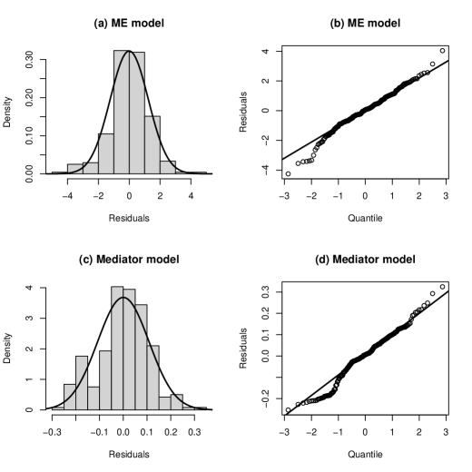
Figure 4: Normality diagnostic plots for the residuals in the measurement error model (4) and mediator model (1). Panel (a): histogram of residuals in the measurement error model (4); Panel (b): QQ plot of residuals in the measurement error model (4); Panel (c): histogram of residuals in the mediator model (1); Panel (d): QQ plot of residuals in the mediator model (1).

We considered the mediation effect measures on the log-hazard ratio scale for a change in physical activity from the lower quartile to the upper quartile of the diary-based METs$\cdot$h$\cdot$wk^-1, conditional on the median levels of the confounding variables. Table 4 (Panel A) presents the estimated mediation effect measures from ORC1, ORC2, RRC, and the uncorrected approaches, based on the approximate mediation effect measure expressions with allowing for an exposure-mediator interaction. The RRC estimator used two equally spaced split points to form the risk sets in the validation study. When $K\geq 3$, the sample size in the last risk set was smaller than 42, which may not be sufficient for providing a stable estimate for the measurement error model (14) given the large number of confounders that need to be considered in the analysis. All methods suggested a negative NIE, NDE, and TE, indicating that VGA leads to a lower risk of cardiovascular diseases. However, the NIE and NDE estimates of the uncorrected method were attenuated towards 0 as compared to the proposed methods, due to exposure measurement error ($\rho_{AA^{*}}=0.62$). The uncorrected approach provided a similar MP estimate to the measurement error corrected approaches, all indicating that about 40% of the total effect from the VGA to CVD was due to BMI. This is not surprising given the bias analysis in Theorem 1 and the observation that the exposure-mediator interaction effect was weak as compared the main effects of the exposure and mediator in outcome model (e.g., ORC1 gives $\widehat{\beta}_{1}^{(O1)}=-0.22$ (S.E: 0.21), $\widehat{\beta}_{2}^{(O1)}=1.31$ (S.E: 0.10), and $\widehat{\beta}_{3}^{(O1)}=0.06$ (S.E: 0.07); ORC2 and RRC also give similar coefficient estimates). Observing that the interaction effect was weak and statistically insignificant, we also included an additional analysis without considering the exposure-mediator interaction effect (See Panel B in Table 4). We found that point estimates without considering interaction were close to their counterparts in Table 4 (Panel A), but the standard errors were smaller.

Table 4: Mediation of the effect of physical activity on cardiovasular diseases incidence by body mass index, with and without considering the exposure-mediator interaction effects, HPFS ($n_{1}=43,547$, $n_{2}=238$), 1986–2016. The mediation effect measures were estimated based on the approximate expressions and were defined on the a log-hazard ratio scale for physical activity increasing from the lower quartile to the upper quartile of the diary-based METs$\cdot$h$\cdot$wk^-1, conditional on the most frequent level/median of the confounding variables.

Method	NIE	NDE	TE	MP
Penal A: with exposure-mediator interaction
Uncorrected	-0.026 (0.003)	-0.038 (0.015)	-0.064 (0.015)	0.401 (0.099)
ORC1	-0.046 (0.006)	-0.066 (0.026)	-0.112 (0.025)	0.412 (0.106)
ORC2	-0.047 (0.006)	-0.065 (0.025)	-0.112 (0.026)	0.421 (0.102)
RRC	-0.047 (0.006)	-0.073 (0.027)	-0.120 (0.027)	0.395 (0.097)
Panel B: without exposure-mediator interaction
Uncorrected	-0.024 (0.002)	-0.038 (0.015)	-0.063 (0.015)	0.389 (0.096)
ORC1	-0.041 (0.004)	-0.068 (0.026)	-0.108 (0.025)	0.377 (0.097)
ORC2	-0.043 (0.004)	-0.066 (0.025)	-0.109 (0.026)	0.391 (0.094)
RRC	-0.042 (0.004)	-0.074 (0.027)	-0.117 (0.027)	0.363 (0.089)

• Numbers in the brackets are the standard errors of the point estimates given by the plug-in estimator of the derived asymptotic variance. The analysis considered the following baseline variables as potential confounders: alcohol intake (yes/no), smoking status (past only/never/current), aspirin use (yes/no), vitamin E supplement use (yes/no), parental history of myocardial infarction at or before 60 years old (yes/no), parental history of cancer at or before 60 years old (yes/no), intake of polyunsaturated fat, trans fat, eicosapentaenoic acid and docosahexaenic acid (g/day), diabetes (yes/no), and hypertension (yes/no).

The cumulative event rate for the CVD is 14.5% in the HPFS, which is technically not a rare outcome. Therefore, the mediation effect measures may be non-constant over time. As a sensitivity analysis, we repeated the mediation analysis in Table 4 (Panel A) using the exact mediation effect measure expressions. Result of $\widehat{\text{NIE}}_{a,a^{*}|\bm{w}}(t)$ is provided in Figure 5. We observed that the estimates given by all approaches were nearly constant with respect to the time ($t$, here, age in months) and were nearly identical to the NIE estimates given in Table 4 (Panel A). Similar results has been observed for the NDE estimates (See Web Figure 2). Therefore, the approximate mediation effect measures we derived served as an adequate approximation to the true mediation effect measures, possibly due to that the cumulative event rate in HPFS (14.5%) was close to 10%, a suggestive threshold for a rare/common outcome.

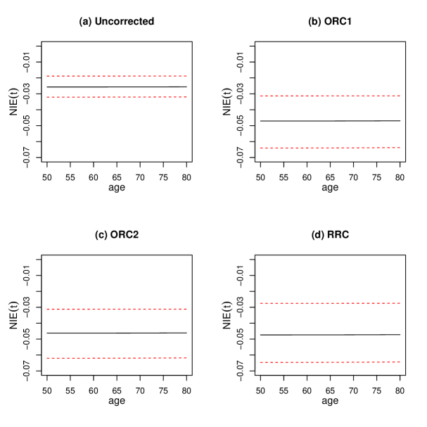
Figure 5: NIE estimates based on the exact mediation effect measure expressions for the HPFS, 1986–2016. The black solid line is the point estimates and the red dotted lines are the 95% confidence interval obtained via bootstrapping.

8 Conclusion

Motivated by the need to account for exposure measurement error in analysis of the HPFS, this article developed correction methods for addressing exposure measurement error-inducted bias in survival mediation analysis. Under a main study/external validation study design, we proposed three approaches, the ORC1, ORC2, and RRC, to provide approximately consistent estimates of the mediation effect measures. Asymptotic properties of these approaches were derived. Simulation studies have confirmed that all of the proposed approaches can effectively remove the bias due to exposure measurement error. Example R code for implementing the proposed methods is available at the Supplementary Material.

As is commonly seen in the literature of measurement error correction in epidemiological studies, this paper considers using linear measurement error models to describe the exposure measurement error process. Sometimes, a linear measurement error model may be not adequate to address the measurement error process. In future work, we plan to consider using more flexible methods (for example, nonparametric and spline approaches) to estimate the measurement error process, and compare its performance to the current methods under correct specification and misspecification of the linear measurement error models.

Since the exact expressions of the mediation effect measures have complex forms that depend on time, we mainly focus on mediation analysis with a rare outcome, where simpler approximate mediation effect measures will be sufficient. Although there is an informal rule of thumb in epidemiology suggesting that events below 10% can be considered rare, there has not been any work published to date that investigates the relative performance of the approximate mediation effect measures under a rare disease assumption when the outcome is common. As in our application study to the HPFS, when the outcome is less rare, we recommend using the exact mediation effect measures, which vary with $t$, to check the robustness of the estimates based on the approximate expressions derived assuming rare disease. If the mediation effect estimates are observed to be nearly constant over time based on the exact expression, one it’s likely that the approximate expressions would be sufficient. Otherwise, one should report the exact mediation effect estimates as defined in (3) and interpret the potentially different results at pre-specified time points of interest.

Supplementary Material

The supplementary material is available at https://sites.google.com/view/chaocheng, which includes web appendices, figures, and tables unshown in the manuscript and example R code for implementing the proposed correction approaches.

References

- Baron and Kenny (1986) Baron, R. M. and Kenny, D. A. (1986), “The moderator–mediator variable distinction in social psychological research: Conceptual, strategic, and statistical considerations.” Journal of Personality and Social Psychology, 51, 1173.
- Carroll et al. (2006) Carroll, R. J., Ruppert, D., Stefanski, L. A., and Crainiceanu, C. M. (2006), Measurement error in nonlinear models: a modern perspective, Chapman and Hall/CRC.
- Chasan-Taber et al. (1996) Chasan-Taber, S., Rimm, E. B., Stampfer, M. J., Spiegelman, D., and et al (1996), “Reproducibility and validity of a self-administered physical activity questionnaire for male health professionals,” Epidemiology, 81–86.
- Cheng et al. (2022) Cheng, C., Spiegelman, D., and Li, F. (2022), “Is the product method more efficient than the difference method for assessing mediation?” American Journal of Epidemiology.
- Cheng et al. (2023) — (2023), “Mediation analysis in the presence of continuous exposure measurement error,” Statistics in Medicine.
- Choi et al. (2005) Choi, H. K., Atkinson, K., Karlson, E. W., and Curhan, G. (2005), “Obesity, weight change, hypertension, diuretic use, and risk of gout in men: the health professionals follow-up study,” Archives of Internal Medicine, 165, 742–748.
- Chomistek et al. (2012) Chomistek, A. K., Cook, N. R., Flint, A. J., and Rimm, E. B. (2012), “Vigorous-intensity leisure-time physical activity and risk of major chronic disease in men,” Medicine and Science in Sports and Exercise, 44, 1898.
- Fernández and Steel (1998) Fernández, C. and Steel, M. F. (1998), “On Bayesian modeling of fat tails and skewness,” Journal of the American Statistical Association, 93, 359–371.
- Lange and Hansen (2011) Lange, T. and Hansen, J. V. (2011), “Direct and indirect effects in a survival context,” Epidemiology, 575–581.
- Liao et al. (2018) Liao, X., Zhou, X., Wang, M., Hart, J. E., Laden, F., and Spiegelman, D. (2018), “Survival analysis with functions of mismeasured covariate histories: the case of chronic air pollution exposure in relation to mortality in the nurses’ health study,” Journal of the Royal Statistical Society: Series C (Applied Statistics), 67, 307–327.
- Liao et al. (2011) Liao, X., Zucker, D., Li, Y., and Spiegelman, D. (2011), “Survival analysis with error-prone time-varying covariates: A risk set calibration approach,” Biometrics, 67, 50–58.
- Liu and Pierce (1994) Liu, Q. and Pierce, D. A. (1994), “A note on Gauss—Hermite quadrature,” Biometrika, 81, 624–629.
- McNutt et al. (2003) McNutt, L.-A., Wu, C., Xue, X., and Hafner, J. P. (2003), “Estimating the relative risk in cohort studies and clinical trials of common outcomes,” American journal of epidemiology, 157, 940–943.
- Prentice (1982) Prentice, R. L. (1982), “Covariate measurement errors and parameter estimation in a failure time regression model,” Biometrika, 69, 331–342.
- Rosner et al. (1990) Rosner, B., Spiegelman, D., and Willett, W. C. (1990), “Correction of logistic regression relative risk estimates and confidence intervals for measurement error: the case of multiple covariates measured with error,” American Journal of Epidemiology, 132, 734–745.
- VanderWeele (2011) VanderWeele, T. J. (2011), “Causal mediation analysis with survival data,” Epidemiology (Cambridge, Mass.), 22, 582.
- Wang and Albert (2017) Wang, W. and Albert, J. M. (2017), “Causal mediation analysis for the Cox proportional hazards model with a smooth baseline hazard estimator,” Journal of the Royal Statistical Society. Series C, Applied statistics, 66, 741.
- Xie et al. (2001) Xie, S. X., Wang, C., and Prentice, R. L. (2001), “A risk set calibration method for failure time regression by using a covariate reliability sample,” Journal of the Royal Statistical Society: Series B (Statistical Methodology), 63, 855–870.
- Yi et al. (2015) Yi, G. Y., Ma, Y., Spiegelman, D., and Carroll, R. J. (2015), “Functional and structural methods with mixed measurement error and misclassification in covariates,” Journal of the American Statistical Association, 110, 681–696.
- Zhao and Prentice (2014) Zhao, S. and Prentice, R. L. (2014), “Covariate measurement error correction methods in mediation analysis with failure time data,” Biometrics, 70, 835–844.