Graph Convex Hull Bounds
as generalized Jensen Inequalities

Abstract

Abstract. Jensen’s inequality is ubiquitous in measure and probability theory, statistics, machine learning, information theory and many other areas of mathematics and data science. It states that, for any convex function $f\colon K\to\mathbb{R}$ on a convex domain $K\subseteq\mathbb{R}^{d}$ and any random variable $X$ taking values in $K$, $\mathbb{E}[f(X)]\geq f(\mathbb{E}[X])$. In this paper, sharp upper and lower bounds on $\mathbb{E}[f(X)]$, termed “graph convex hull bounds”, are derived for arbitrary functions $f$ on arbitrary domains $K$, thereby strongly generalizing Jensen’s inequality. Establishing these bounds requires the investigation of the convex hull of the graph of $f$, which can be difficult for complicated $f$. On the other hand, once these inequalities are established, they hold, just like Jensen’s inequality, for any random variable $X$. Hence, these bounds are of particular interest in cases where $f$ is fairly simple and $X$ is complicated or unknown. Both finite- and infinite-dimensional domains and codomains of $f$ are covered, as well as analogous bounds for conditional expectations and Markov operators.

Keywords. Jensen’s inequality $\bullet$ Convex Hull $\bullet$ non-convex functions $\bullet$ Markov operators $\bullet$ conditional expectation $\bullet$ Hahn–Banach separation theorem

2020 Mathematics Subject Classification. 26D15 $\bullet$ 28B05 $\bullet$ 46A55 $\bullet$ 52A40 $\bullet$ 60B11 $\bullet$ 37A30

FUBFreie Universität Berlin, Arnimallee 6, 14195 Berlin, Germany ()

1 Introduction

In many theoretical and practical derivations, it is often not possible to exactly compute the mean $\mathbb{E}[f(X)]$ of a function $f\colon K\to\mathbb{R}$, $K\subseteq\mathbb{R}^{d}$, $d\in\mathbb{N}$, applied to a $K$-valued random variable $X$, so one has to rely on bounds on $\mathbb{E}[f(X)]$. This is particularly the case when $X$ is only known in terms of its mean $\mathbb{E}[X]$ and one has to rely solely on the knowledge of $\mathbb{E}[X]$ and $f$, leading to the following general problem formulation addressed in this paper:

Problem 1.1.

Establish (sharp) bounds on the mean $\mathbb{E}[f(X)]$ given $\mathbb{E}[X]$ and $f$.

In this finite-dimensional setup, Jensen’s inequality (Jensen, 1906) provides partial answers for convex functions $f$ on convex domains $K$, in which case it states that

$$\mathbb{E}[f(X)]\geq f(\mathbb{E}[X])$$ (1.1)

(note that no upper bound is given). While Jensen’s inequality is one of the fundamental results in measure theory and is used ubiquitously in probability theory, statistics, information theory, statistical physics and many other research areas, it still has some crucial limitations and restrictions. The aim of this paper is to derive new bounds on $\mathbb{E}[f(X)]$, termed graph convex hull bounds, that remedy these shortcomings, in particular:

• Jensen’s inequality says nothing about functions $f$ that are neither convex nor concave, while the graph convex hull bounds hold for arbitrary functions.

• While Jensen’s inequality requires a convex domain $K$ of $f$, the graph convex hull bounds have no restrictions on the domain — it may even be disconnected, cf.  Example 3.9 and Figure 3.1.

• Jensen’s inequality provides no “reverse” bounds of the forms $\mathbb{E}[f(X)]\leq s+f(\mathbb{E}[X])$ or $\mathbb{E}[f(X)]\leq cf(\mathbb{E}[X])$ for some $s=s(X)\geq 0$, $c=c(X)\geq 1$, even though this is relevant in numerous situations and can certainly be obtained for specific functions or function classes (Wunder et al., 2021; Dragomir, 2013; Khan et al., 2020b; Budimir et al., 2001). The minimal value $s=s(X)\geq 0$ which satisfies above property is called the Jensen gap (Abramovich and Persson, 2016; Ullah et al., 2021; Khan et al., 2020a). The graph convex hull bounds provide sharp bounds on $\mathbb{E}[f(X)]$ both from above and below. However, unlike the Jensen gap, our bounds depend on $X$ only through $\mathbb{E}[X]$ (cf. 1.1), hence they are more generally applicable but can only be sharp in a weaker sense.

• If $K$ is a subset of an infinite-dimensional topological vector space $\mathcal{X}$, then some form of continuity assumption on $f$ is necessary for Jensen’s inequality to hold (Perlman, 1974), while the graph convex hull bounds do not require any continuity assumptions.

The graph convex hull bounds are obtained by exploiting the basic fact that the mean of the pair $(X,f(X))$ lies in the closure $\overline{\operatorname{Conv}(\mathcal{G}(f))}$ of the convex hull of the graph $\mathcal{G}(f)$ of $f$, cf. Corollary 3.3 and Figure 3.1 below, and the proof is a simple application of the Hahn–Banach separation theorem — characterize $\overline{\operatorname{Conv}(\mathcal{G}(f))}$ as an intersection of half-spaces and note that the expected value $\mathbb{E}$ as an operator “respects” each half-space, since it is linear, positive and $\mathbb{E}[Z]=Z$ for constant $Z$. While the graph convex hull bounds in concrete applications require some investigation of $\overline{\operatorname{Conv}(\mathcal{G}(f))}$ (note that Jensen’s inequality also requires some analysis of $f$, namely the verification of its convexity), all inequalities are derived solely from the properties of $f$ and hold, just like Jensen’s inequality, for any random variable $X$ no matter its probability distribution. This property is crucial since, in practice, the function $f$ is often sufficiently simple to analyze (at least numerically), while the random variable $X$ might not be simple or even well known; or one requires a statement that holds for all such random variables simultaneously.

Note that the three properties of $\mathbb{E}$ mentioned above for the derivation of $(\mathbb{E}[X],\mathbb{E}[f(X)])\in\overline{\operatorname{Conv}(\mathcal{G}(f))}$ are of algebraic nature and have little to do with measure or integration theory. Hence, the graph convex hull bounds can be extended to a larger class of linear operators in place of $\mathbb{E}$, so-called Markov operators, as well as to conditional expectations, which are well-known facts in the case of Jensen’s inequality, see e.g. (Bakry et al., 2014, Equation (1.2.1)) and (Dudley, 2002, Theorem 10.2.7). Once these three versions of the graph convex hull bounds are proven, the corresponding versions of Jensen’s inequality follow as simple corollaries, providing a novel and considerably simpler proof of this famous result (cf. Remark 3.12). By working in a more general setup than is typical for Markov operators (Remark 4.2), we also strongly generalize the corresponding version of Jensen’s inequality.

The paper is structured as follows. After introducing the general setup and notation in Section 2, the graph convex hull bounds for expected values are derived in Section 3, the ones for Markov operators in Section 4 and the ones for conditional expectations in Section 5. The corresponding versions of Jensen’s inequality are derived as Corollaries 3.11, 4.11, and 5.7 in each of the three sections separately.

2 Preliminaries

In order to formulate the results in the most general setting possible, we assume that $\mathcal{X}$ and $\mathcal{Y}$ are real, Hausdorff, locally convex topological vector spaces and $f\colon K\to\mathcal{Y}$, $K\subseteq\mathcal{X}$, but the reader is welcome to think of $\mathcal{X}=\mathbb{R}^{d}$ and $\mathcal{Y}=\mathbb{R}$. Further, $(\Omega,\Sigma,\mathbb{P})$ will denote a probability space and $X\colon\Omega\to\mathcal{X}$ be such that $(X,f(X))$ is weakly integrable; and all expected values are to be understood in the weak sense (in particular, $X$ does not necessarily have to be measurable, i.e. a random variable). Recall that a map $X\colon\Omega\to\mathcal{X}$ is called weakly integrable if there exists $e\in\mathcal{X}$ such that, for any $\ell\in\mathcal{X}^{\prime}$, $\ell(X)\in L^{1}(\mathbb{P})$ and $\ell(e)=\int_{\Omega}\ell(X)\,\mathrm{d}\mathbb{P}$, in which case the expected value of $X$ is defined by $\mathbb{E}[X]\coloneqq\int_{\Omega}X\,\mathrm{d}\mathbb{P}\coloneqq e$ (Rudin, 1991, Definition 3.26). Here, $\mathcal{X}^{\prime}$ denotes the continuous dual of $\mathcal{X}$. In particular, each Pettis or Bochner integrable map is weakly integrable and the reader is welcome to think of Bochner integrable random variables $X$. When working with Markov operators in Section 4, no measurability or integrability assumptions will be imposed on $(X,f(X))$, while for conditional expectations in Section 5 we will assume $\mathcal{X}$ and $\mathcal{Y}$ to be Banach spaces and $(X,f(X))$ to be Bochner integrable. Recall that a random variable $X\colon(\Omega,\Sigma,\mathbb{P})\to\mathcal{X}$ is Bochner or strongly integrable if and only if $X$ is measurable and $\int_{\mathcal{X}}\lVert X\rVert_{\mathcal{X}}\,\mathrm{d}\mathbb{P}<\infty$ (Diestel and Uhl, 1977, Theorem II.2.2), in which case we write $X\in L^{1}(\mathbb{P};\mathcal{X})$. The specific assumptions will be introduced in each section separately, see Assumptions 3.1, 4.5, and 5.1.

Throughout the paper, we use the following notation. We denote the closure of a subset $A$ of a real topological vector space by $\overline{A}$ and the convex hull of $A$ by

$$\operatorname{Conv}(A)\coloneqq\bigcap\{C\supset A\mid C\text{ convex}\}=\left\{\textstyle\sum_{j=1}^{J}w_{j}a_{j}\,\middle|\,J\in\mathbb{N},\,a_{j}\in A,\,w_{j}\geq 0,\,\textstyle\sum_{j=1}^{J}w_{j}=1\right\}.$$ (2.1)

Further, $\mathcal{G}(f)=\{(x,f(x))\mid x\in K\}$ denotes the graph of a function $f\colon K\to\mathcal{Y}$ and, for $M\subseteq\mathcal{X}\times\mathcal{Y}$ and $x\in\mathcal{X}$,

$$M|_{x}\coloneqq\{y\in\mathcal{Y}\mid(x,y)\in M\}$$

(note that $\overline{M}|_{x}$ and $\overline{M|_{x}}$ might not coincide). Finally, while we clearly have in mind inequalities with respect to some total or partial order or preorder on $\mathcal{Y}$, most statements are formulated for arbitrary binary relations on $\mathcal{Y}$, which we still denote by $\leq$ for readability reasons. However, in the case $\mathcal{Y}=\mathbb{R}$ we always assume the canonical total order. In certain situations, we will extend the space $\mathcal{Y}$ by adding the elements $\pm\infty$, which we assume to satisfy $-\infty\leq y\leq\infty$ for each $y\in\mathcal{Y}$, and write $\overline{\mathcal{Y}}\coloneqq\mathcal{Y}\cup\{\pm\infty\}$, as is typical for the extended real number line $\overline{\mathbb{R}}=[-\infty,\infty]=\mathbb{R}\cup\{\pm\infty\}$. Closed intervals in $\overline{\mathcal{Y}}$ are defined by $[a,b]\coloneqq\{y\in\overline{\mathcal{Y}}\mid a\leq y\leq b\},\ a,b\in\overline{\mathcal{Y}}.$ We now state a simple preliminary lemma that we will use to derive Jensen’s inequality from the graph convex hull bounds:

Lemma 2.1.

Let $f\colon K\to\mathbb{R}$ be a convex function on a convex domain $K\subseteq\mathbb{R}^{d}$. Then its epigraph $\operatorname{epi}(f)\coloneqq\{(x,y)\in K\times\mathbb{R}\mid y\geq f(x)\}\supseteq\mathcal{G}(f)$ is convex and, consequently, $\operatorname{Conv}(\mathcal{G}(f))|_{x}\subseteq[f(x),\infty)$ for each $x\in K$. If $K=\mathbb{R}^{d}$, then $\overline{\operatorname{Conv}(\mathcal{G}(f))}|_{x}\subseteq[f(x),\infty)$ for each $x\in K$.

Proof. Let $(x_{1},y_{1}),(x_{2},y_{2})\in\operatorname{epi}(f)$ and $\lambda\in[0,1]$ be arbitrary. Then, since $K$ is convex by assumption, $x_{\ast}\coloneqq\lambda x_{1}+(1-\lambda)x_{2}\in K$. Further, by definition of the epigraph and by convexity of $f$,

$$y_{\ast}\coloneqq\lambda y_{1}+(1-\lambda)y_{2}\geq\lambda f(x_{1})+(1-\lambda)f(x_{2})\geq f(\lambda x_{1}+(1-\lambda)x_{2})=f(x_{\ast}).$$

Hence, $(x_{\ast},y_{\ast})=\lambda(x_{1},y_{1})+(1-\lambda)(x_{2},y_{2})\in\operatorname{epi}(f)$, proving convexity of $\operatorname{epi}(f)$. It follows that $\operatorname{Conv}(\mathcal{G}(f))\subseteq\operatorname{epi}(f)$ by (2.1) and $\operatorname{Conv}(\mathcal{G}(f))|_{x}\subseteq\operatorname{epi}(f)|_{x}=[f(x),\infty)$ for each $x\in K$. If $K=\mathbb{R}^{d}$, then $f$ is continuous (Borwein and Lewis, 2006, Theorem 4.1.3) and $\operatorname{epi}(f)$ is closed. Hence, $\overline{\operatorname{Conv}(\mathcal{G}(f))}|_{x}\subseteq\overline{\operatorname{epi}(f)}|_{x}=\operatorname{epi}(f)|_{x}=[f(x),\infty)$ for each $x\in K$. $\blacksquare$

3 Graph Convex Hull Bounds for Expected Values

Throughout this section, we make the following general assumptions:

Assumption 3.1.

$(\Omega,\Sigma,\mathbb{P})$ is a probability space, $\mathcal{X},\mathcal{Y},\mathcal{Z}$ are real, Hausdorff, locally convex topological vector spaces (equipped with their Borel $\sigma$-algebras). Further, $\leq$ is any binary relation on $\mathcal{Y}$, which we assume to be the canonical total order in the case $\mathcal{Y}=\mathbb{R}$ (hence the notation). Finally, $K\subseteq\mathcal{X}$, $f\colon K\to\mathcal{Y}$ and $X\colon\Omega\to K$ such that the pair $(X,f(X))$ is weakly integrable.

The following theorem is a well-known and intuitive result that the mean $\mathbb{E}[Z]$ of a random variable $Z$ taking values in a closed convex subset $C$ of $\mathcal{Z}$ lies within this set: $\mathbb{E}[Z]\in C$. If $\mathcal{Z}=\mathbb{R}^{d}$, the closedness assumption can be dropped. Its proof is based on the Hahn–Banach separation theorem.

Theorem 3.2 (mean/barycenter of convex set lies within its closure).

Let Assumption 3.1 hold and let $Z\colon\Omega\to A$ be a weakly integrable map taking values in a subset $A\subseteq\mathcal{Z}$. Then $\mathbb{E}[Z]\in\operatorname{Conv}(A)$ if $\mathcal{Z}=\mathbb{R}^{d}$, $d\in\mathbb{N}$, and $\mathbb{E}[Z]\in\overline{\operatorname{Conv}(A)}$ in general. Further, for any $z\in\operatorname{Conv}(A)$ there exist a probability space $(\tilde{\Omega},\tilde{\Sigma},\tilde{\mathbb{P}})$ and a weakly integrable map $\tilde{Z}\colon\tilde{\Omega}\to A$ such that $\mathbb{E}[\tilde{Z}]=z$.

Proof. See (Perlman, 1974, Theorem 3.1) for the general statement $\mathbb{E}[Z]\in\overline{\operatorname{Conv}(A)}$ and (Dudley, 2002, Theorem 10.2.6.) for the proof of $\mathbb{E}[Z]\in\operatorname{Conv}(A)$ in the case $\mathcal{Z}=\mathbb{R}^{d}$ (though our setup is slightly more general, the proof goes similarly). Now let $z\in\operatorname{Conv}(A)$. Then it can be written as a convex combination of elements of $A$, i.e. $z=\sum_{j=1}^{J}w_{j}a_{j},$ for some $J\in\mathbb{N}$, $a_{j}\in A$, $w_{j}\geq 0$, $j=1,\dots,J$, with $\sum_{j=1}^{J}w_{j}=1$. Choose $\tilde{\Omega}=\{1,\dots,J\}$ with distribution $\tilde{\mathbb{P}}$ given by the probability vector $(w_{1},\dots,w_{J})$ and let $\tilde{Z}(j)=a_{j}$. Then $\mathbb{E}[\tilde{Z}]=\sum_{j=1}^{J}w_{j}a_{j}=z$. $\blacksquare$

An application of above theorem to the convex hull of the graph of a function $f$ yields:

Corollary 3.3.

Under Assumption 3.1, $\mathbb{E}[(X,f(X))]\in\operatorname{Conv}(\mathcal{G}(f))$ if $\mathcal{X}=\mathbb{R}^{m},\,\mathcal{Y}=\mathbb{R}^{n},\ m,n\in\mathbb{N}$, and $\mathbb{E}[(X,f(X))]\in\overline{\operatorname{Conv}(\mathcal{G}(f))}$ in general. Further, for any $(x,y)\in\operatorname{Conv}(\mathcal{G}(f))$ there exist a probability space $(\tilde{\Omega},\tilde{\Sigma},\tilde{\mathbb{P}})$ and $\tilde{X}\colon\tilde{\Omega}\to K$ such that the pair $(\tilde{X},f(\tilde{X}))$ is weakly integrable and $\mathbb{E}[(\tilde{X},f(\tilde{X}))]=(x,y)$.

Proof. This follows from Theorem 3.2 for $Z\coloneqq(X,f(X))$ and $A\coloneqq\mathcal{G}(f)\subseteq\mathcal{X}\times\mathcal{Y}\eqqcolon\mathcal{Z}$ (note that any map $\tilde{Z}$ taking values in $\mathcal{G}(f)$ is of the form $(\tilde{X},f(\tilde{X}))$). $\blacksquare$

The following result is basically a restatement of Corollary 3.3. Since it is the main result of this section, we state it as a theorem:

Theorem 3.4 (graph convex hull bounds on $\mathbb{E}[f(X)]$).

Under Assumption 3.1, let the convex hull of the graph of $f$ be “enclosed” by two “envelope” functions $g_{l},g_{u}\colon\overline{\operatorname{Conv}(K)}\to\overline{\mathcal{Y}}$ in the following way:

$$\begin{split}\overline{\operatorname{Conv}(\mathcal{G}(f))}&\subseteq\{(x,y)\in\overline{\operatorname{Conv}(K)}\times\mathcal{Y}\mid g_{l}(x)\leq y\leq g_{u}(x)\},\\[4.30554pt] \text{i.e.}\qquad\overline{\operatorname{Conv}(\mathcal{G}(f))}|_{x}&\subseteq[g_{l}(x),g_{u}(x)]\qquad\text{for each }x\in\overline{\operatorname{Conv}(K)}.\end{split}$$ (3.1)

Then

$$g_{l}(\mathbb{E}[X])\leq\mathbb{E}[f(X)]\leq g_{u}(\mathbb{E}[X]).$$ (3.2)

If $\mathcal{X}=\mathbb{R}^{m},\,\mathcal{Y}=\mathbb{R}^{n},\ m,n\in\mathbb{N}$, then $\overline{\operatorname{Conv}(K)}$ and $\overline{\operatorname{Conv}(\mathcal{G}(f))}$ can be replaced by $\operatorname{Conv}(K)$ and $\operatorname{Conv}(\mathcal{G}(f))$, respectively. Further, for $\mathcal{Y}=\mathbb{R}$, (3.2) is sharp in the following sense:

• If $\mathcal{X}=\mathbb{R}^{m}$ and $g_{l}(x)=\inf(\operatorname{Conv}(\mathcal{G}(f))|_{x})$ and $g_{u}(x)=\sup(\operatorname{Conv}(\mathcal{G}(f))|_{x})$ for each $x\in\operatorname{Conv}(K)$, then, for every $x\in\operatorname{Conv}(K)$ and $y\in(g_{l}(x),g_{u}(x))$, there exist a probability space $(\tilde{\Omega},\tilde{\Sigma},\tilde{\mathbb{P}})$ and $\tilde{X}\colon\tilde{\Omega}\to K$ such that the pair $(\tilde{X},f(\tilde{X}))$ is weakly integrable and $(\mathbb{E}[\tilde{X}],\mathbb{E}[f(\tilde{X})])=(x,y)$.

• In general, if $g_{l}(x)=\inf(\overline{\operatorname{Conv}(\mathcal{G}(f))}|_{x})$ and $g_{u}(x)=\sup(\overline{\operatorname{Conv}(\mathcal{G}(f))}|_{x})$ for each $x\in\overline{\operatorname{Conv}(K)}$, then, for every $x\in\overline{\operatorname{Conv}(K)}$ and $y\in(g_{l}(x),g_{u}(x))$ and for any neighborhood $U$ of $(x,y)$, there exist a probability space $(\tilde{\Omega},\tilde{\Sigma},\tilde{\mathbb{P}})$ and $\tilde{X}\colon\tilde{\Omega}\to K$ such that the pair $(\tilde{X},f(\tilde{X}))$ is weakly integrable and $(\mathbb{E}[\tilde{X}],\mathbb{E}[f(\tilde{X})])\in U$.

Proof. Since $\mathbb{E}[X]\in\overline{\operatorname{Conv}(K)}$ and $(\mathbb{E}[X],\mathbb{E}[f(X)])\in\overline{\operatorname{Conv}(\mathcal{G}(f))}$ by Theorems 3.2 and 3.3,

$$\mathbb{E}[f(X)]\in\overline{\operatorname{Conv}(\mathcal{G}(f))}|_{\mathbb{E}[X]}\subseteq[g_{l}(\mathbb{E}[X]),g_{u}(\mathbb{E}[X])],$$

cf. Figure 3.1. In the finite-dimensional case $\mathcal{X}=\mathbb{R}^{m},\,\mathcal{Y}=\mathbb{R}^{n}$, we can omit all the closures by Theorems 3.2 and 3.3. The claim on the sharpness of the bounds also follows directly from Corollary 3.3. $\blacksquare$

Remark 3.5.

Again we wish to stress that, just like Jensen’s inequality, the bounds $g_{l}$ and $g_{u}$ depend solely on the function $f$ and hold for any $K$-valued map $X$ satisfying the minimal integrability assumptions.

Note that the lower bound $f(\mathbb{E}[X])$ on $\mathbb{E}[f(X)]$ in Jensen’s inequality (1.1) is superfluous in our setup and may not even be well defined (note that $\mathbb{E}[X]\notin K$ is possible, cf. Example 3.9). However, if a comparison between $\mathbb{E}[f(X)]$ and $f(\mathbb{E}[X])$ is of the essence, the above result has the following consequences whenever $f(\mathbb{E}[X])$ exists:

Corollary 3.6.

Let the assumptions of Theorem 3.4 hold and let $\mathcal{Y}=\mathbb{R}$. Then

1. $c_{l}(\mathbb{E}[X])\,f(\mathbb{E}[X])\leq\mathbb{E}[f(X)]\leq c_{u}(\mathbb{E}[X])\,f(\mathbb{E}[X])$,

2. $\max\big{(}\inf_{x\in K}f(x)\,,\,f(\mathbb{E}[X])-s_{u}\big{)}\leq\mathbb{E}[f(X)]\leq\min\big{(}\sup_{x\in K}f(x)\,,\,f(\mathbb{E}[X])+s_{l}\big{)},$

3. $\hat{c}_{l}\,f(\mathbb{E}[X])\leq\mathbb{E}[f(X)]\leq\hat{c}_{u}\,f(\mathbb{E}[X])$,

whenever the quantities

$$c_{l}(x) \coloneqq\tfrac{g_{l}(x)}{f(x)}, s_{l} \coloneqq\lVert f-g_{l}\rVert_{\infty}, \hat{c}_{l} \coloneqq\inf_{x\in\overline{\operatorname{Conv}(K)}}\tfrac{g_{l}(x)}{f(x)},$$

$$c_{u}(x) \coloneqq\tfrac{g_{u}(x)}{f(x)}, s_{u} \coloneqq\lVert f-g_{u}\rVert_{\infty}, \hat{c}_{u} \coloneqq\sup_{x\in\overline{\operatorname{Conv}(K)}}\tfrac{g_{u}(x)}{f(x)},$$

as well as $f(\mathbb{E}[X])$ are well defined. If $\mathcal{X}=\mathbb{R}^{m},\,\mathcal{Y}=\mathbb{R}^{n},\ m,n\in\mathbb{N}$, $\overline{\operatorname{Conv}(K)}$ can be replaced by $\operatorname{Conv}(K)$ in the definition of $\hat{c}_{l}$ and $\hat{c}_{u}$.

Proof. (a) and (b) follow directly from Theorem 3.4, while (c) follows from (a). $\blacksquare$

Remark 3.7.

While the bounds in Theorem 3.4 and Corollary 3.6 (a) require the knowledge of $\mathbb{E}[X]$ (cf. 1.1), the weaker statements (b) and (c) compare $\mathbb{E}[f(X)]$ with $f(\mathbb{E}[X])$ without using this information. However, they still provide sharper bounds than the obvious inequalities (whenever well defined)

$$\inf_{x\in K}f(x)\leq\mathbb{E}[f(X)]\leq\sup_{x\in K}f(x),\qquad f(\mathbb{E}[X])\inf_{x,y\in\overline{K}}\tfrac{f(x)}{f(y)}\leq\mathbb{E}[f(X)]\leq f(\mathbb{E}[X])\sup_{x,y\in\overline{K}}\tfrac{f(x)}{f(y)}.$$

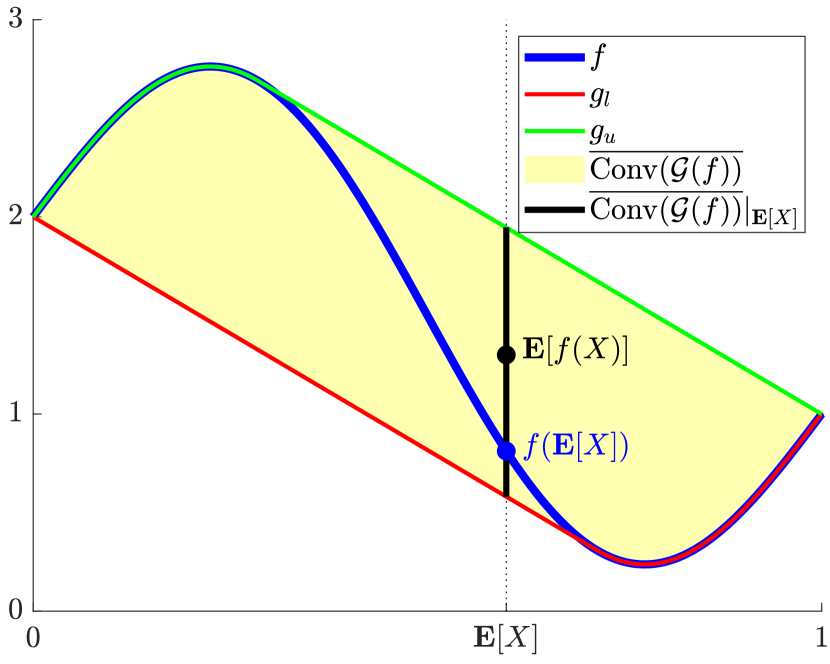
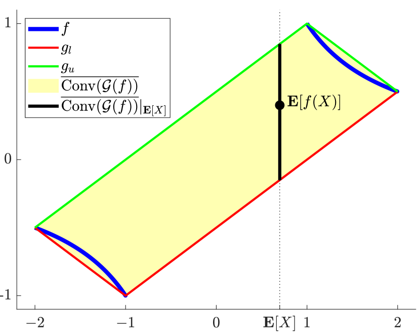
Figure 3.1: Illustration of Examples 3.8 and 3.9. Since the mean $\mathbb{E}[(X,f(X))]=(\mathbb{E}[X],\mathbb{E}[f(X)])$ (black dot) of the pair $(X,f(X))$ lies in the closure $\overline{\operatorname{Conv}(\mathcal{G}(f))}$ of the convex hull of the graph of $f$, the value $\mathbb{E}[f(X)]$ is restricted to the thick black line $\overline{\operatorname{Conv}}_{\mathbb{E}[X]}$, providing the bounds in Theorem 3.4. Note that, in the second example, the domain $K=[-2,-1]\cup[1,2]$ of $f$ is disconnected and $f(\mathbb{E}[X])$ is not even defined whenever $\mathbb{E}[X]\in(-1,1)$, which has no influence on Theorem 3.4.

Example 3.8.

Let $K=[0,1]$ and $f\colon K\to\mathbb{R}$, $f(x)=2-x+\sin(2\pi x)$, visualized in Figure 3.1 (left), which is neither convex nor concave. Then the “envelope” functions of $\operatorname{Conv}(\mathcal{G}(f))$ are given by

$$g_{l}(x)=\begin{cases}2-ax&\text{if }x\leq x_{\ast},\\ f(x)&\text{otherwise},\end{cases}\qquad g_{u}(x)=\begin{cases}f(x)&\text{if }x\leq x_{\ast},\\ 1+a-ax&\text{otherwise},\end{cases}$$

where $x_{\ast}\approx 0.715$ is the solution of $2\pi\cos(2\pi x)\,x=\sin(2\pi x)$ and $a=1-2\pi\cos(2\pi x_{\ast})$. Note that the constants $\hat{c}_{l}\approx 0.5$ and $\hat{c}_{u}\approx 6.5$ from Corollary 3.6 compare favorably with the obvious bounds $\inf_{x,y\in K}\tfrac{f(x)}{f(y)}\approx 0.09$ and $\sup_{x,y\in K}\tfrac{f(x)}{f(y)}\approx 11.6.$ from Remark 3.5 (it is easy to see how the function $f$ can be modified to make the improvements over these bounds as large as desired).

Example 3.9.

Let $K=[-2,-1]\cup[1,2]$ be the disconnected domain of the function $f\colon K\to\mathbb{R}$, $f(x)=x^{-1}$, visualized in Figure 3.1 (right), which again is neither convex nor concave. Again, the “envelope” functions of $\operatorname{Conv}(\mathcal{G}(f))$ from Theorem 3.4, given by the piecewise linear functions

$$g_{l}(x)=\begin{cases}(-3-x)/2&\text{if }x\in[-2,-1],\\ (x-1)/2&\text{if }x\in[-1,-2],\end{cases}\qquad g_{u}(x)=\begin{cases}(3-x)/2&\text{if }x\in[-2,1],\\ (x-1)/2&\text{if }x\in[1,2],\end{cases}$$

provide sharp bounds on $\mathbb{E}[f(X)]$. In this case, it might be impossible to compare $\mathbb{E}[f(X)]$ with $f(\mathbb{E}[X])$, since the latter is not defined whenever $\mathbb{E}[X]\in(-1,1)$.

Remark 3.10.

While in the above examples the envelope functions $g_{l}$ and $g_{u}$ were established analytically (up to the approximation of $x_{\ast}$), they usually can be computed numerically with high precision and little computational effort even for a complicated function $f$, as long as its domain $K$ is bounded.

We end this section by showing that the graph convex hull bounds from Theorem 3.4 imply Jensen’s inequality:

Corollary 3.11 (Jensen’s inequality).

Let Assumption 3.1 hold and $f\colon K\to\mathbb{R}$ be a convex function on a convex domain $K\subseteq\mathbb{R}^{d}$. Then $\mathbb{E}[f(X)]\geq f(\mathbb{E}[X])$.

Proof. This follows directly from Theorem 3.4 and Lemma 2.1. $\blacksquare$

Remark 3.12.

Note that this novel proof strategy of Jensen’s inequality is considerably simpler than the conventional one: In the proof of e.g. (Dudley, 2002, Theorem 10.2.6.), the author provides

• a first argument showing $\mathbb{E}[X]\in K$, similar to Theorem 3.2, so $f(\mathbb{E}[X])$ is well defined,

• a second simple argument similar to Lemma 2.1 and

• a third, lengthy argument proving the inequality itself.

However, the third argument can be avoided completely by applying the first argument a second time, this time to the pair $(X,f(X))$, yielding $(\mathbb{E}[X],\mathbb{E}[f(X)])\in\operatorname{Conv}(\mathcal{G}(f))$ and almost immediately proving Jensen’s inequality. This simple line of argumentation seems to have been overlooked in the past, as well as its generalization to non-convex functions and domains as in Theorem 3.4.

4 Graph Convex Hull Bounds for Markov Operators

Note that the only properties of the expected value $\mathbb{E}$ used to prove $\mathbb{E}[Z]\in\overline{\operatorname{Conv}(A)}$ in Theorem 3.2 are linearity, positivity of $\ell(Z)$ for each $\ell\in\mathcal{Z}^{\prime}$ (i.e. $\ell(Z)\geq 0$ implies $\mathbb{E}[\ell(Z)]\geq 0$) as well as $\mathbb{E}[Z]=Z$ for each constant random variable $Z\in\mathcal{Z}$ (and the same is true for Jensen’s inequality). Therefore, Jensen’s inequality and the graph convex hull bounds can be seen as algebraic results rather than measure theoretic ones, and can be extended to operators that do not necessarily involve integration, but simply satisfy the three properties above. Such a generalization is the purpose of this section and it will also allow us to cover conditional expectations in the subsequent section. Such operators are known as Markov operators and play a crucial role in the analysis of time evolution phenomena and dynamical systems (Bakry et al., 2014). It is well-known that they satisfy Jensen’s inequality (Bakry et al., 2014, Equation (1.2.1)).

Definition 4.1.

Let $\Omega_{1},\Omega_{2}$ be sets and $\mathcal{S}_{1},\mathcal{S}_{2}$ be vector spaces of functions on $\Omega_{1}$ and $\Omega_{2}$ that contain the unit constant functions $\mathds{1}_{\Omega_{1}}\colon\Omega_{1}\to\mathbb{R}$, $t\mapsto 1$ and $\mathds{1}_{\Omega_{2}}$, respectively, e.g. $\mathcal{S}_{1}=L^{1}(\mathbb{P}_{1})$, if $(\Omega_{1},\Sigma_{1},\mathbb{P}_{1})$ is a probability space. A linear operator $\mathcal{E}\colon\mathcal{S}_{1}\to\mathcal{S}_{2}$ is called a Markov operator if

1. $\mathcal{E}(\mathds{1}_{\Omega_{1}})=\mathds{1}_{\Omega_{2}}$,

2. $\mathcal{E}(\varphi)\geq 0$ for each $\varphi\in\mathcal{S}_{1}$ with $f\geq 0$.

Further, let $\mathcal{Z}$ be a real topological vector space and

$$\mathcal{S}^{\mathcal{Z}}_{1}\subseteq\{Z_{1}\colon\Omega_{1}\to\mathcal{Z}\mid\ell\in\mathcal{Z}^{\prime}\colon\ell(Z_{1})\in\mathcal{S}_{1}\},\quad\mathcal{S}^{\mathcal{Z}}_{2}\subseteq\{Z_{2}\colon\Omega_{2}\to\mathcal{Z}\mid\ell\in\mathcal{Z}^{\prime}\colon\ell(Z_{2})\in\mathcal{S}_{2}\},$$

e.g. $\mathcal{S}^{\mathcal{Z}}_{1}=L^{1}(\mathbb{P}_{1};\mathcal{Z})$ in the case $\mathcal{S}_{1}=L^{1}(\mathbb{P}_{1})$. We call $\mathcal{E}^{\mathcal{Z}}\colon\mathcal{S}^{\mathcal{Z}}_{1}\to\mathcal{S}^{\mathcal{Z}}_{2}$ a $\mathcal{Z}$-valued Markov operator associated with the Markov operator $\mathcal{E}$ if $\ell(\mathcal{E}^{\mathcal{Z}}(Z_{1}))=\mathcal{E}(\ell(Z_{1}))$ for each $\ell\in\mathcal{Z}^{\prime}$ and $Z_{1}\in\mathcal{S}^{\mathcal{Z}}_{1}$, i.e.  if the following diagram commutes for each $\ell\in\mathcal{Z}^{\prime}$.

Remark 4.2.

Typically, $\Omega_{1},\Omega_{2}$ are assumed to be measurable spaces or measure spaces, and the elements in $\mathcal{S}_{1},\mathcal{S}_{2}$ to be measurable or to lie in $L^{1}$ with respect to certain measures (Bakry et al., 2014; Eisner et al., 2015). Further, some authors require Markov operators to be endomorphisms, i.e. $\mathcal{S}_{1}=\mathcal{S}_{2}$ (Bakry et al., 2014), to be $L^{1}$-contractions (Lin, 1979; Rudnicki, 2000) or to be $L^{1}$-norm preserving (Eisner et al., 2015). By working under the minimal requirements in Definition 4.1 and by introducing the entirely new notion of a $\mathcal{Z}$-valued Markov operator, we therefore strongly generalize the presently known version of Jensen’s inequality for Markov operators (Bakry et al., 2014, Equation (1.2.1)).

Example 4.3 (cf. Section 3).

Let $(\Omega_{1},\Sigma_{1},\mathbb{P}_{1})=(\Omega_{2},\Sigma_{2},\mathbb{P}_{2})$ be a probability space and $\mathcal{S}_{1}=L^{1}(\mathbb{P}_{1})$ and $\mathcal{S}_{2}=\operatorname{span}(\mathds{1}_{\Omega_{2}})$. Further, let $\mathcal{Z}$ be a real, Hausdorff, locally convex topological vector space and $\mathcal{S}^{\mathcal{Z}}_{1}=\{Z_{1}\colon\Omega_{1}\to\mathcal{Z}\mid Z_{1}\text{ weakly integrable}\}$, $\mathcal{S}^{\mathcal{Z}}_{2}=\{Z_{2}\colon\Omega_{2}\to\mathcal{Z}\mid Z_{2}\text{ constant}\}$. Then the expected value $\mathbb{E}\colon\mathcal{S}^{\mathcal{Z}}_{1}\to\mathcal{S}^{\mathcal{Z}}_{2}$ is a $\mathcal{Z}$-valued Markov operator associated with the Markov operator $\mathbb{E}\colon\mathcal{S}_{1}\to\mathcal{S}_{2}$, where $\mathcal{S}^{\mathcal{Z}}_{2}$ is identified with $\mathcal{Z}$ and $\mathcal{S}_{2}$ with $\mathbb{R}$. Note that the same notation $\mathbb{E}$ is used for both operators as is the standard in probability theory.

Example 4.4 (cf. Section 5).

Let $(\Omega_{1},\Sigma_{1},\mathbb{P}_{1})=(\Omega_{2},\Sigma_{2},\mathbb{P}_{2})$ be a probability space and $\mathcal{F}\subseteq\Sigma_{1}$ be a sub-$\sigma$-algebra of $\Sigma_{1}$. Let $\mathcal{S}_{1}=L^{1}(\Sigma_{1},\mathbb{P}_{1})$ and $\mathcal{S}_{2}=L^{1}(\mathcal{F},\mathbb{P}_{1}|_{\mathcal{F}})$. Further, let $\mathcal{Z}$ be a Banach space, $\mathcal{S}^{\mathcal{Z}}_{1}=L^{1}(\Sigma_{1},\mathbb{P}_{1};\mathcal{Z})$ and $\mathcal{S}^{\mathcal{Z}}_{2}=L^{1}(\mathcal{F},\mathbb{P}|_{\mathcal{F}};\mathcal{Z})$. Then the conditional expectation $\mathbb{E}[\mathchoice{\mathbin{\vbox{\hbox{\scalebox{0.5}{$\;\displaystyle\bullet\;$}}}}}{\mathbin{\vbox{\hbox{\scalebox{0.5}{$\;\textstyle\bullet\;$}}}}}{\mathbin{\vbox{\hbox{\scalebox{0.5}{$\;\scriptstyle\bullet\;$}}}}}{\mathbin{\vbox{\hbox{\scalebox{0.5}{$\;\scriptscriptstyle\bullet\;$}}}}}|\mathcal{F}]\colon\mathcal{S}^{\mathcal{Z}}_{1}\to\mathcal{S}^{\mathcal{Z}}_{2}$ is a $\mathcal{Z}$-valued Markov operator associated with the Markov operator $\mathbb{E}[\mathchoice{\mathbin{\vbox{\hbox{\scalebox{0.5}{$\;\displaystyle\bullet\;$}}}}}{\mathbin{\vbox{\hbox{\scalebox{0.5}{$\;\textstyle\bullet\;$}}}}}{\mathbin{\vbox{\hbox{\scalebox{0.5}{$\;\scriptstyle\bullet\;$}}}}}{\mathbin{\vbox{\hbox{\scalebox{0.5}{$\;\scriptscriptstyle\bullet\;$}}}}}|\mathcal{F}]\colon\mathcal{S}_{1}\to\mathcal{S}_{2}$ (this follows easily from e.g. (Diestel and Uhl, 1977, Theorem II.2.6)). Again, the same notation $\mathbb{E}[\mathchoice{\mathbin{\vbox{\hbox{\scalebox{0.5}{$\;\displaystyle\bullet\;$}}}}}{\mathbin{\vbox{\hbox{\scalebox{0.5}{$\;\textstyle\bullet\;$}}}}}{\mathbin{\vbox{\hbox{\scalebox{0.5}{$\;\scriptstyle\bullet\;$}}}}}{\mathbin{\vbox{\hbox{\scalebox{0.5}{$\;\scriptscriptstyle\bullet\;$}}}}}|\mathcal{F}]$ is used for both operators as is common practice.

In order to generalize the results in Section 3 to Markov operators, we introduce the following assumptions for this section:

Assumption 4.5.

$\mathcal{X},\mathcal{Y}$ are two real, Hausdorff, locally convex topological vector spaces and $\Omega_{1},\,\Omega_{2},\,\mathcal{S}_{1},\,\mathcal{S}_{2},\,\mathcal{S}^{\mathcal{X}}_{1},\,\mathcal{S}^{\mathcal{X}}_{2},\,\mathcal{S}^{\mathcal{Y}}_{1},\,\mathcal{S}^{\mathcal{Y}}_{2}$ are as in Definition 4.1, with $\mathcal{Z}$ replaced by $\mathcal{X}$ and $\mathcal{Y}$, respectively. Further, $\mathcal{E}^{\mathcal{X}}\colon\mathcal{S}^{\mathcal{X}}_{1}\to\mathcal{S}^{\mathcal{X}}_{2}$ and $\mathcal{E}^{\mathcal{Y}}\colon\mathcal{S}^{\mathcal{Y}}_{1}\to\mathcal{S}^{\mathcal{Y}}_{2}$ are $\mathcal{X}$-valued and $\mathcal{Y}$-valued Markov operators, respectively, associated with the same Markov operator $\mathcal{E}\colon\mathcal{S}_{1}\to\mathcal{S}_{2}$. $\leq$ is any binary relation on $\mathcal{Y}$, which we assume to be the canonical total order in the case $\mathcal{Y}=\mathbb{R}$. Finally $K\subseteq\mathcal{X}$, $f\colon K\to\mathcal{Y}$ and $X\colon\Omega_{1}\to K$ such that the pair $(X,f(X))\in\mathcal{S}^{\mathcal{X}}_{1}\times\mathcal{S}^{\mathcal{Y}}_{1}$.

Lemma 4.6.

Under Assumption 4.5, the operator $\mathcal{E}^{\mathcal{X}\times\mathcal{Y}}\colon\mathcal{S}^{\mathcal{X}}_{1}\times\mathcal{S}^{\mathcal{Y}}_{1}\to\mathcal{S}^{\mathcal{X}}_{2}\times\mathcal{S}^{\mathcal{Y}}_{2},\ (\tilde{X},\tilde{Y})\mapsto(\mathcal{E}^{\mathcal{X}}(\tilde{X}),\mathcal{E}^{\mathcal{Y}}(\tilde{Y}))$ is an $(\mathcal{X}\times\mathcal{Y})$-valued Markov operator associated with the same Markov operator $\mathcal{E}$.

Proof. Let $\tilde{Z}=(\tilde{X},\tilde{Y})\in\mathcal{S}^{\mathcal{X}}_{1}\times\mathcal{S}^{\mathcal{Y}}_{1}$ and $\ell\in(\mathcal{X}\times\mathcal{Y})^{\prime}$. Then $\ell$ is of the form $\ell(x,y)=\ell^{\mathcal{X}}(x)+\ell^{\mathcal{Y}}(y)$ for some $\ell^{\mathcal{X}}\in\mathcal{X}^{\prime},\,\ell^{\mathcal{Y}}\in\mathcal{Y}^{\prime}$. Hence, $\ell(\tilde{Z})=\ell^{\mathcal{X}}(\tilde{X})+\ell^{\mathcal{Y}}(\tilde{Y})\in\mathcal{S}$ (since $\mathcal{S}$ is a vector space), as required (and similarly for $\mathcal{S}^{\mathcal{X}}_{2}\times\mathcal{S}^{\mathcal{Y}}_{2}$). Further,

$$\ell(\mathcal{E}^{\mathcal{X}\times\mathcal{Y}}(\tilde{Z}))=\ell^{\mathcal{X}}(\mathcal{E}^{\mathcal{X}}(\tilde{X})+\ell^{\mathcal{Y}}(\mathcal{E}^{\mathcal{Y}}(\tilde{Y})=\mathcal{E}(\ell^{\mathcal{X}}(\tilde{X}))+\mathcal{E}(\ell^{\mathcal{Y}}(\tilde{Y}))=\mathcal{E}(\ell(\tilde{Z})).$$

$\blacksquare$

Let us now formulate the analogue of Theorem 3.2 for Markov operators:

Theorem 4.7 (Markov operators respect closed convex set constraints).

Let $\Omega_{1},\,\Omega_{2},\,\mathcal{S}_{1},\,\mathcal{S}_{2},\,\mathcal{E}$, $\mathcal{Z},\ \mathcal{S}^{\mathcal{Z}}_{1},\,\mathcal{S}^{\mathcal{Z}}_{2},\,\mathcal{E}^{\mathcal{Z}}$ be as in Definition 4.1 and assume that $\mathcal{Z}$ is Hausdorff and locally convex. Further, let $Z\in\mathcal{S}_{1}$ with $Z(\Omega_{1})\subseteq A$ for some subset $A\subseteq\mathcal{Z}$. Then $(\mathcal{E}^{\mathcal{Z}}(Z))(\Omega_{2})\subseteq\overline{\operatorname{Conv}(A)}$.

Proof. By the Hahn–Banach separation theorem, since $\overline{\operatorname{Conv}(A)}$ is convex, it coincides with the intersection of all closed half-spaces $\mathcal{H}_{\ell,s}\coloneqq\{z\in\mathcal{Z}\mid\ell(z)\geq s\}\supseteq\overline{\operatorname{Conv}(A)}$ including it, where $\ell\in\mathcal{Z}^{\prime}\setminus\{0\}$ and $s\in\mathbb{R}$. Since, for $\omega\in\Omega$,

$$Z(\Omega_{1})\subseteq\mathcal{H}_{\ell,s} \implies\ell(Z)\geq s$$

$$\implies\mathcal{E}(\ell(Z))\geq s$$

$$\implies\ell(\mathcal{E}^{\mathcal{Z}}(Z)\geq s$$

$$\implies\mathcal{E}^{\mathcal{Z}}(Z)(\Omega_{2})\subseteq\mathcal{H}_{\ell,s},$$

$(\mathcal{E}^{\mathcal{Z}}(Z))(\Omega_{2})$ lies in each half-space $\mathcal{H}_{\ell,s}$ including $\overline{\operatorname{Conv}(A)}$, proving the claim. $\blacksquare$

An application of above theorem to the convex hull of the graph of a function $f$ yields:

Corollary 4.8.

Under Assumption 5.1, $(\mathcal{E}^{\mathcal{X}}(X),\mathcal{E}^{\mathcal{Y}}(f(X)))(\Omega_{2})\subseteq\overline{\operatorname{Conv}(\mathcal{G}(f))}$.

Proof. Using Lemma 4.6, this follows from Theorem 4.7 for $Z\coloneqq(X,f(X))$ and $A\coloneqq\mathcal{G}(f)\subseteq\mathcal{X}\times\mathcal{Y}\eqqcolon\mathcal{Z}$. $\blacksquare$

As in Section 3, a reformulation of above corollary results in graph convex hull bounds for Markov operators in place of expected values:

Theorem 4.9 (graph convex hull bounds on $\mathcal{E}^{\mathcal{Y}}(f(X))$).

Under Assumption 5.1, let the convex hull of the graph of $f$ be “enclosed” by two “envelope” functions $g_{l},g_{u}\colon\overline{\operatorname{Conv}(K)}\to\overline{\mathcal{Y}}$ satisfying (3.1). Then

$$g_{l}(\mathcal{E}^{\mathcal{X}}(X))\leq\mathcal{E}^{\mathcal{Y}}(f(X))\leq g_{u}(\mathcal{E}^{\mathcal{X}}(X)).$$ (4.1)

Note that, in contrast to Theorem 3.4, all objects in (4.1) are functions on $\Omega_{2}$.

Proof. Since $(\mathcal{E}^{\mathcal{X}}(X))(\Omega_{2})\subseteq\overline{\operatorname{Conv}(K)}$ and $(\mathcal{E}^{\mathcal{X}}(X),\mathcal{E}^{\mathcal{Y}}(f(X)))(\Omega_{2})\subseteq\overline{\operatorname{Conv}(\mathcal{G}(f))}$ by Theorems 4.7 and 4.8,

$$(\mathcal{E}^{\mathcal{Y}}(f(X)))(\Omega_{2})\subseteq\overline{\operatorname{Conv}(\mathcal{G}(f))}|_{\mathcal{E}^{\mathcal{X}}(X)}\subseteq[g_{l}(\mathcal{E}^{\mathcal{X}}(X)),g_{u}(\mathcal{E}^{\mathcal{X}}(X))].$$

$\blacksquare$

Corollary 4.10.

Let the assumptions of Theorem 4.9 hold and let $\mathcal{Y}=\mathbb{R}$. Then, using the notation from Corollary 3.6,

1. $c_{l}(\mathcal{E}^{\mathcal{X}}(X))\,f(\mathcal{E}^{\mathcal{X}}(X))\leq\mathcal{E}^{\mathcal{Y}}(f(X))\leq c_{u}(\mathcal{E}^{\mathcal{X}}(X))\,f(\mathcal{E}^{\mathcal{X}}(X))$,

2. $\max\big{(}\inf_{x\in K}f(x)\,,\,f(\mathcal{E}^{\mathcal{X}}(X))-s_{u}\big{)}\leq\mathcal{E}^{\mathcal{Y}}(f(X))\leq\min\big{(}\sup_{x\in K}f(x)\,,\,f(\mathcal{E}^{\mathcal{X}}(X))+s_{l}\big{)},$

3. $\hat{c}_{l}\,f(\mathcal{E}^{\mathcal{X}}(X))\leq\mathcal{E}^{\mathcal{Y}}(f(X))\leq\hat{c}_{u}\,f(\mathcal{E}^{\mathcal{X}}(X))$,

whenever these quantities are well defined.

Proof. (a) and (b) follow directly from Theorem 4.9, while (c) follows from (a). $\blacksquare$

Again, we end this section by obtaining Jensen’s inequality as a simple corollary of Theorem 4.9. To the best of the author’s knowledge, Jensen’s inequality for Markov operators has not yet been derived in this generality, cf. Remark 4.2.

Corollary 4.11 (Jensen’s inequality for Markov operators).

Let Assumption 4.5 hold and $f\colon\mathbb{R}^{d}\to\mathbb{R}$ be a convex function. Then $\mathcal{E}^{\mathcal{Y}}(f(X))\geq f(\mathcal{E}^{\mathcal{X}}(X))$.

Proof. This follows directly from Theorem 4.9 and Lemma 2.1. $\blacksquare$

5 Graph Convex Hull Bounds for Conditional Expectations

It is well-known that Jensen’s inequality also holds for conditional expectations (Dudley, 2002, Theorem 10.2.7). In this section, we derive graph convex hull bounds for conditional expectations, which is a special case of the general setup in Section 4 (cf. Example 4.4) and will follow from the results therein. Since conditional expectations are typically defined over Banach spaces and for Bochner integrable random variables (Diestel and Uhl, 1977, Section V.1), this will require slightly stronger assumptions:

Assumption 5.1.

$(\Omega,\Sigma,\mathbb{P})$ is a probability space, $\mathcal{X},\mathcal{Y},\mathcal{Z}$ are real Banach spaces and $K\subseteq\mathcal{X}$ a subset of $\mathcal{X}$. Further, $\leq$ is any binary relation on $\mathcal{Y}$, which we assume to be the canonical total order in the case $\mathcal{Y}=\mathbb{R}$ and $\mathcal{F}\subseteq\Sigma$ is a sub-$\sigma$-algebra with $\mathbb{E}[\mathchoice{\mathbin{\vbox{\hbox{\scalebox{0.5}{$\;\displaystyle\bullet\;$}}}}}{\mathbin{\vbox{\hbox{\scalebox{0.5}{$\;\textstyle\bullet\;$}}}}}{\mathbin{\vbox{\hbox{\scalebox{0.5}{$\;\scriptstyle\bullet\;$}}}}}{\mathbin{\vbox{\hbox{\scalebox{0.5}{$\;\scriptscriptstyle\bullet\;$}}}}}|\mathcal{F}]$ denoting the corresponding conditional expectation. Finally, $K\subseteq\mathcal{X}$, $f\colon K\to\mathbb{R}$ and $X\colon\Omega\to K$ is a random variable such that the pair $(X,f(X))$ is Bochner integrable.

Theorem 5.2 (conditional expectations respect closed convex set constraints).

Let $Z\colon(\Omega,\Sigma,\mathbb{P})\to A$ be a Bochner integrable random variable taking values in a subset $A\subseteq\mathcal{Z}$ of a real Banach space $\mathcal{Z}$ and let $\mathcal{F}\subseteq\Sigma$ be a sub-$\sigma$-algebra. Then $\mathbb{E}[Z|\mathcal{F}]\in\overline{\operatorname{Conv}(A)}$ $\mathbb{P}$-almost surely.

Proof. Note that, as is typical for conditional expectations, no difference is made in the notation between $\mathbb{E}[\mathchoice{\mathbin{\vbox{\hbox{\scalebox{0.5}{$\;\displaystyle\bullet\;$}}}}}{\mathbin{\vbox{\hbox{\scalebox{0.5}{$\;\textstyle\bullet\;$}}}}}{\mathbin{\vbox{\hbox{\scalebox{0.5}{$\;\scriptstyle\bullet\;$}}}}}{\mathbin{\vbox{\hbox{\scalebox{0.5}{$\;\scriptscriptstyle\bullet\;$}}}}}|\mathcal{F}]\colon L^{1}(\Sigma,\mathbb{P})\to L^{1}(\mathcal{F},\mathbb{P}|_{\mathcal{F}})$ and $\mathbb{E}[\mathchoice{\mathbin{\vbox{\hbox{\scalebox{0.5}{$\;\displaystyle\bullet\;$}}}}}{\mathbin{\vbox{\hbox{\scalebox{0.5}{$\;\textstyle\bullet\;$}}}}}{\mathbin{\vbox{\hbox{\scalebox{0.5}{$\;\scriptstyle\bullet\;$}}}}}{\mathbin{\vbox{\hbox{\scalebox{0.5}{$\;\scriptscriptstyle\bullet\;$}}}}}|\mathcal{F}]\colon L^{1}(\Sigma,\mathbb{P};\mathcal{Z})\to L^{1}(\mathcal{F},\mathbb{P}|_{\mathcal{F}};\mathcal{Z})$ (corresponding to $\mathcal{E}$ and $\mathcal{E}_{\mathcal{Z}}$ in Definition 4.1). Since $\mathbb{E}[\ell(Z)|\mathcal{F}]=\ell(\mathbb{E}[Z|\mathcal{F}])$ for each $\ell\in\mathcal{Z}^{\prime}$ (this follows easily from e.g. (Diestel and Uhl, 1977, Theorem II.2.6)), and that $W\geq s$ implies $\mathbb{E}[W|\mathcal{F}]\geq s$ $\mathbb{P}$-almost surely for each real-valued random variable $W\colon(\Omega,\Sigma,\mathbb{P})\to\mathbb{R}$ by (Kallenberg, 2021, Theorem 8.1(ii)), the claim follows directly from Theorem 4.7. $\blacksquare$

Remark 5.3.

In contrast to Section 4, all statements in $L^{1}$ can only hold $\mathbb{P}$-almost surely. Hence, when drawing the transferring the final conclusion from the proof of Theorem 4.7 to the one of Theorem 5.2, we have to be slightly careful when taking the intersection over all (possibly uncountably many) half-spaces including $\overline{\operatorname{Conv}(A)}$. However, following the construction of conditional expectations (Diestel and Uhl, 1977, Theorem V.1.4), there exists a representative of $\mathbb{E}[Z|\mathcal{F}]$ which lies in all these half-spaces simultaneously.

An application of above theorem to the convex hull of the graph of a function $f$ yields:

Corollary 5.4.

Under Assumption 5.1, $\mathbb{E}[(X,f(X))|\mathcal{F}]\in\overline{\operatorname{Conv}(\mathcal{G}(f))}$ $\mathbb{P}$-almost surely.

Proof. This follows from Theorem 5.2 for $Z\coloneqq(X,f(X))$ and $A\coloneqq\mathcal{G}(f)\subseteq\mathcal{X}\times\mathcal{Y}\eqqcolon\mathcal{Z}$. $\blacksquare$

Theorem 5.5 (graph convex hull bounds on $\mathbb{E}[f(X)|\mathcal{F}]$).

Under Assumption 5.1, let the convex hull of the graph of $f$ be “enclosed” by two “envelope” functions $g_{l},g_{u}\colon\overline{\operatorname{Conv}(K)}\to\overline{\mathcal{Y}}$ satisfying (3.1). Then

$$g_{l}(\mathbb{E}[X|\mathcal{F}])\leq\mathbb{E}[f(X)|\mathcal{F}]\leq g_{u}(\mathbb{E}[X|\mathcal{F}])\text{ $\mathbb{P}$-almost surely}.$$ (5.1)

Note that, in contrast to Theorem 3.4, all objects in (5.1) are random variables.

Proof. Since $\mathbb{E}[X|\mathcal{F}]\in\overline{\operatorname{Conv}(K)}$ $\mathbb{P}$-almost surely and $(\mathbb{E}[X|\mathcal{F}],\mathbb{E}[f(X)|\mathcal{F}])\in\overline{\operatorname{Conv}(\mathcal{G}(f))}$ $\mathbb{P}$-almost surely by Theorems 5.2 and 5.4,

$$\mathbb{E}[f(X)|\mathcal{F}]\subseteq\overline{\operatorname{Conv}(\mathcal{G}(f))}|_{\mathbb{E}[X|\mathcal{F}]}\subseteq[g_{l}(\mathbb{E}[X|\mathcal{F}]),g_{u}(\mathbb{E}[X|\mathcal{F}])]\text{ $\mathbb{P}$-almost surely}.$$

$\blacksquare$

Corollary 5.6.

Let the assumptions of Theorem 5.5 hold and let $\mathcal{Y}=\mathbb{R}$. Then, using the notation from Corollary 3.6,

1. $c_{l}(\mathbb{E}[X|\mathcal{F}])\,f(\mathbb{E}[X|\mathcal{F}])\leq\mathbb{E}[f(X)]\leq c_{u}(\mathbb{E}[X|\mathcal{F}])\,f(\mathbb{E}[X|\mathcal{F}])$,

2. $\max\big{(}\inf_{x\in K}f(x)\,,\,f(\mathbb{E}[X|\mathcal{F}])-s_{u}\big{)}\leq\mathbb{E}[f(X)]\leq\min\big{(}\sup_{x\in K}f(x)\,,\,f(\mathbb{E}[X|\mathcal{F}])+s_{l}\big{)},$

3. $\hat{c}_{l}\,f(\mathbb{E}[X|\mathcal{F}])\leq\mathbb{E}[f(X)]\leq\hat{c}_{u}\,f(\mathbb{E}[X|\mathcal{F}])$,

$\mathbb{P}$-almost surely, whenever these quantities are well defined.

Proof. (a) and (b) follow directly from Theorem 5.5, while (c) follows from (a). $\blacksquare$

Again, conditional Jensen’s inequality follows almost directly from Theorem 5.5:

Corollary 5.7 (conditional Jensen’s inequality).

Let Assumption 5.1 hold and $f\colon\mathbb{R}^{d}\to\mathbb{R}$ be a convex function. Then $\mathbb{E}[f(X)|\mathcal{F}]\geq f(\mathbb{E}[X|\mathcal{F}])$ $\mathbb{P}$-almost surely.

Proof. This follows directly from Theorem 5.5 and Lemma 2.1. $\blacksquare$

References

- Abramovich and Persson (2016) S. Abramovich and L.-E. Persson. Some new estimates of the ‘Jensen gap’. J. Inequal. Appl., pages Paper No. 39, 9, 2016. 10.1186/s13660-016-0985-4.
- Bakry et al. (2014) D. Bakry, I. Gentil, and M. Ledoux. Analysis and geometry of Markov diffusion operators, volume 348 of Grundlehren der mathematischen Wissenschaften [Fundamental Principles of Mathematical Sciences]. Springer, Cham, 2014. 10.1007/978-3-319-00227-9.
- Borwein and Lewis (2006) J. M. Borwein and A. S. Lewis. Convex analysis and nonlinear optimization, volume 3 of CMS Books in Mathematics/Ouvrages de Mathématiques de la SMC. Springer, New York, second edition, 2006. 10.1007/978-0-387-31256-9. Theory and examples.
- Budimir et al. (2001) I. Budimir, S. S. Dragomir, and J. Pečarić. Further reverse results for Jensen’s discrete inequality and applications in information theory. JIPAM. J. Inequal. Pure Appl. Math., 2(1):Article 5, 14, 2001.
- Diestel and Uhl (1977) J. Diestel and J. J. Uhl. Vector Measures, volume 15 of Mathematical Surveys. American Mathematical Society, Providence, RI, 1977. 10.1090/surv/015.
- Dragomir (2013) S. S. Dragomir. Some reverses of the Jensen inequality with applications. Bull. Aust. Math. Soc., 87(2):177–194, 2013. 10.1017/S0004972712001098.
- Dudley (2002) R. M. Dudley. Real analysis and probability, volume 74 of Cambridge Studies in Advanced Mathematics. Cambridge University Press, Cambridge, 2002. 10.1017/CBO9780511755347. Revised reprint of the 1989 original.
- Eisner et al. (2015) T. Eisner, B. Farkas, M. Haase, and R. Nagel. Operator theoretic aspects of ergodic theory, volume 272 of Graduate Texts in Mathematics. Springer, Cham, 2015. 10.1007/978-3-319-16898-2.
- Jensen (1906) J. L. W. V. Jensen. Sur les fonctions convexes et les inégalités entre les valeurs moyennes. Acta Math., 30(1):175–193, 1906. 10.1007/BF02418571.
- Kallenberg (2021) O. Kallenberg. Foundations of modern probability, volume 99 of Probability Theory and Stochastic Modelling. Springer, Cham, 2021. 10.1007/978-3-030-61871-1. Third edition.
- Khan et al. (2020a) S. Khan, M. Adil Khan, S. I. Butt, and Y.-M. Chu. A new bound for the Jensen gap pertaining twice differentiable functions with applications. Adv. Difference Equ., pages Paper No. 333, 11, 2020a. 10.1186/s13662-020-02794-8.
- Khan et al. (2020b) S. Khan, M. Adil Khan, and Y.-M. Chu. Converses of the Jensen inequality derived from the Green functions with applications in information theory. Math. Methods Appl. Sci., 43(5):2577–2587, 2020b. 10.1002/mma.6066.
- Lin (1979) M. Lin. Weak mixing for semigroups of Markov operators without finite invariant measures. In Ergodic theory (Proc. Conf., Math. Forschungsinst., Oberwolfach, 1978), volume 729 of Lecture Notes in Math., pages 89–92. Springer, Berlin, 1979. 10.1007/BFb0063286.
- Perlman (1974) M. D. Perlman. Jensen’s inequality for a convex vector-valued function on an infinite-dimensional space. J. Multivariate Anal., 4:52–65, 1974. 10.1016/0047-259X(74)90005-0.
- Phelps (2001) R. R. Phelps. Lectures on Choquet’s theorem, volume 1757 of Lecture Notes in Mathematics. Springer-Verlag, Berlin, second edition, 2001. 10.1007/b76887.
- Rudin (1991) W. Rudin. Functional analysis. International Series in Pure and Applied Mathematics. McGraw-Hill, Inc., New York, second edition, 1991.
- Rudnicki (2000) R. Rudnicki. Markov operators: applications to diffusion processes and population dynamics. volume 27, pages 67–79. 2000. 10.4064/am-27-1-67-79. Dedicated to the memory of Wiesław Szlenk.
- Ullah et al. (2021) H. Ullah, M. Adil Khan, and T. Saeed. Determination of bounds for the jensen gap and its applications. Mathematics, 9(23), 2021. 10.3390/math9233132.
- Wunder et al. (2021) G. Wunder, B. Groß, R. Fritschek, and R. F. Schaefer. A reverse Jensen inequality result with application to mutual information estimation. In 2021 IEEE Information Theory Workshop (ITW), pages 1–6, 2021. 10.1109/ITW48936.2021.9611449.