Detection Transformer with Stable Matching

Abstract

This paper is concerned with the matching stability problem across different decoder layers in DEtection TRansformers (DETR). We point out that the unstable matching in DETR is caused by a multi-optimization path problem, which is highlighted by the one-to-one matching design in DETR. To address this problem, we show that the most important design is to use and only use positional metrics (like IOU) to supervise classification scores of positive examples. Under the principle, we propose two simple yet effective modifications by integrating positional metrics to DETR’s classification loss and matching cost, named position-supervised loss and position-modulated cost. We verify our methods on several DETR variants. Our methods show consistent improvements over baselines. By integrating our methods with DINO, we achieve $50.4$ and $51.5$ AP on the COCO detection benchmark using ResNet-50 backbones under $1\times$ (12 epochs) and $2\times$ (24 epochs) training settings, achieving a new record under the same setting. We achieve 63.8 AP on COCO detection test-dev with a Swin-Large backbone. Our code will be made available at https://github.com/IDEA-Research/Stable-DINO.

1 Introduction

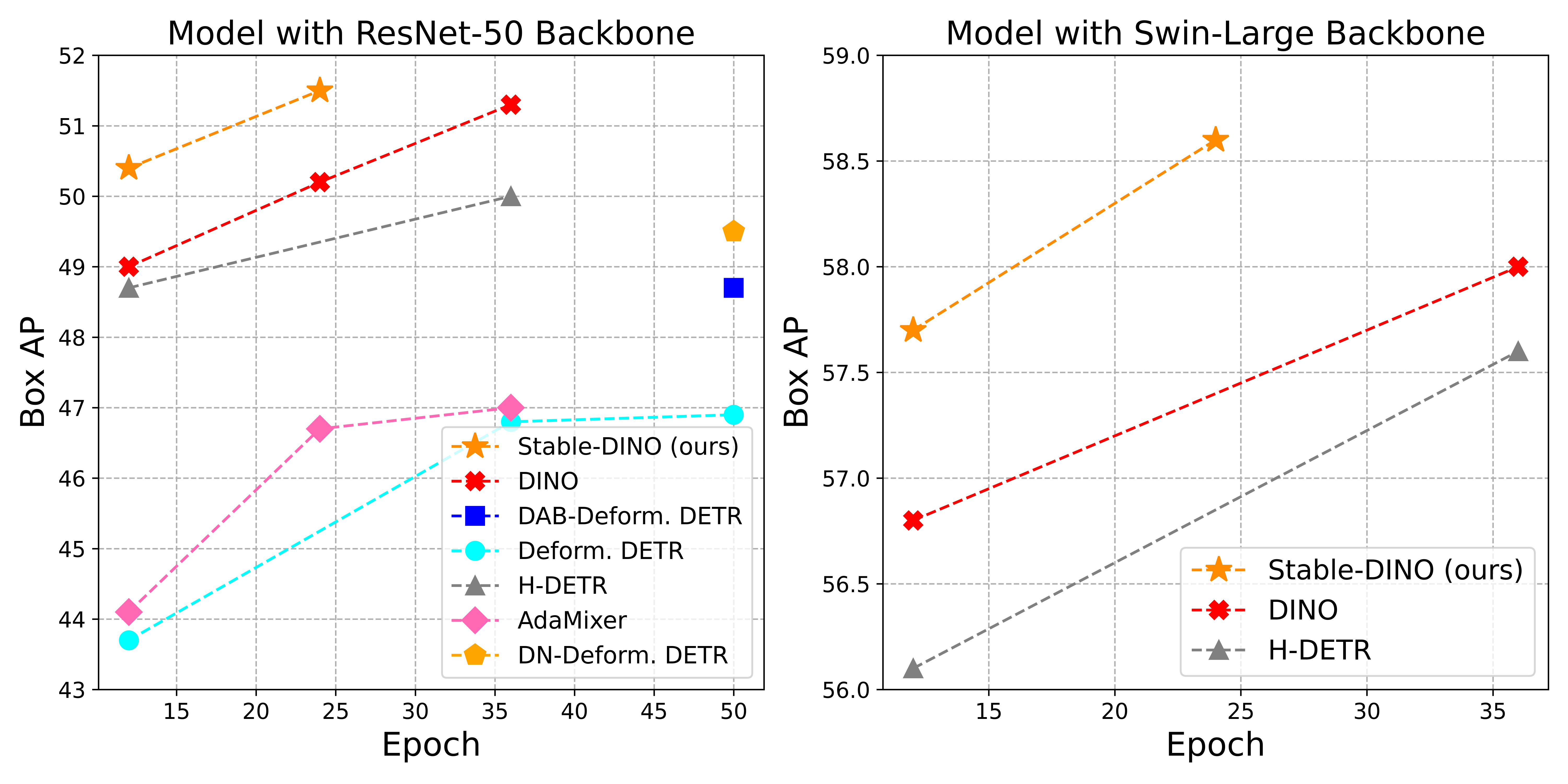
Figure 1: Comparison of our methods (named Stable-DINO in figures) and baselines. We compare models with ResNet-50 backbones in the left figure and models with Swin-Transformer Large backbones in the right figure. All models use a maximum $1/8$ resolution feature map from a backbone, except AdaMixer uses a maximum $1/4$ resolution feature map.

Object detection is a fundamental task in vision with wide applications. Great progress has been made in the last decades with the development of deep learning, especially the convolutional neural network (CNN) [36, 14, 16, 7].

Detection Transformer (DETR) [3] proposed a novel Transformer-based object detector, which attracted a lot of interest in the research community. It gets rid of the need for all hand-crafted modules and enables end-to-end training. One key design in DETR is the matching strategy, which uses Hungarian matching to one-to-one assign predictions to ground truth labels. Despite its novel designs, DETR also has certain limitations associated with this innovative approach, including slow convergence and inferior performance. Many follow-ups tried to improve DETR from many perspectives, like introducing positional prior [32, 41, 28, 14], extra positive examples [22, 4, 5], and efficient operators [47, 34]. With many optimizations, DINO [46] set a new record on the COCO detection leaderboard, making the Transformer-based method become a main-stream detector for large-scale training.

Although DETR-like detectors achieve impressive performance, one critical issue that has received insufficient attention to date, which may potentially compromise the model training stability. This issue pertains to the unstable matching problem across different decoder layers. DETR-like models stack multiple decoder layers in the Transformer decoder. The models assign predictions and calculate losses after each decoder layer. However, the labels assigned to these predictions may differ across different layers. This discrepancy may lead to conflict optimization targets under the one-to-one matching strategy of DETR variants, where each ground truth label is matched with only one prediction.

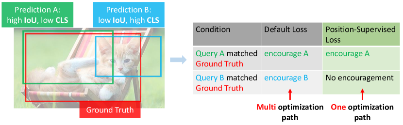
Figure 2: Explanation of the multi-optimization path problem. We use the term “CLS” as classification scores. Each prediction has a probability to be assigned as the positive example in bipartite matching and be encouraged towards ground truth during training, which can be different optimization paths. With the position-supervised loss, only one optimization path will have in the training, which can stabilize the matching.

To the best of our knowledge, only one work [22] has attempted to address the issue of unstable matching problem to date. DN-DETR [22] proposed a novel de-noising training approach by introducing extra hard-assigned queries to avoid mismatching. Some other work [19, 5] added extra queries for faster convergence but did not focus on the unstable matching problem. In contrast, we solve this problem by focusing on the matching and loss calculation process.

We present that the key to the unstable matching problem is the multi-optimization path problem. As shown in Fig. 2, there are two imperfect predictions during training. Prediction A has a higher Intersection over Union (IoU) score but a lower classification score, while prediction B is the opposite. This is the simplest but most common case during training. The model will assign one of them to the ground truth, resulting in two optimization preferences: one that encourages A, which means encouraging predictions with high positional metrics to get better classification results, and the other is to encourage B, which means encouraging predictions with high semantic metrics (classification scores here) to get better IOU scores. We refer to these preferences as different optimization paths. Due to the randomness during training, each prediction has a probability of being assigned as a positive example, with the other being viewed as a negative example. Given the default loss designs, whether A or B is selected as the positive example, the model will optimize it towards its alignment with the ground truth bounding box, which means the model has multi-optimization paths, as shown in the right table in Fig. 2. This issue is less significant in traditional detectors, as multiple queries will be selected as positive examples. However, the one-to-one matching in DETR-like models magnifies the optimization gap between predictions A and B, which makes model training less efficient.

To solve the problem, we find the most critical design is to use and only use positional metrics (e.g., IOU) to supervise the classification scores of positive examples. More formal presentations are available in Sec. 2.2. If we use position information to constrain classification scores, the prediction B will not be encouraged if it is matched since it has a low IoU score. As a result, only one optimization path will be available, mitigating the multi-optimization paths issue. If extra classification score-related supervision is introduced, the multi-optimization path will still impair the model performance, since the prediction B has a better classification score. With this principle, we propose two simple but effective modifications to the loss and matching cost: position-supervised loss and position-modulated cost. Both of them enable faster convergence and better performance of models. Our proposed approach also establishes a link between DETR-like models and traditional detectors, as both encourage predictions with high positional scores to have better classification scores. More detailed analyses are available in Sec. 2.4.

Moreover, we have observed that fusing the backbone and encoder features of models can facilitate the utilization of the pre-trained backbone features, leading to faster convergence, especially in early training iterations, and better performance of models with nearly no extra costs. We propose three fusion ways and empirically select the dense memory fusion for the experiments. See Sec. 3 for more details.

We verify our methods on several different DETR variants. Our methods show consistent improvement in all experiments. We then build a strong detector named Stable-DINO by combining our methods with DINO. Stable-DINO presents impressive results on the COCO detection benchmark. The comparison between our model and other DETR variants is shown in Fig. 1. Stable-DINO achieves $50.4$ and $51.5$ AP with four feature scales from a ResNet-50 backbone under $1\times$ and $2\times$ training schedulers, with $+1.4$ and $+1.1$ AP gains compared with DINO baselines. With a stronger backbone Swin Transformer Large, Stable-DINO can achieve $57.7$ and $58.6$ AP with $1\times$ and $2\times$ training schedulers. To the best of our knowledge, these are the best results among DETR variants under the same settings.

2 Stable Matching

This section presents our solution to the unstable matching problem in DETR-like models. We first review the loss functions and matching strategies in previous work (Sec. 2.1). To solve the unstable matching problem, we demonstrate our modifications on losses and matching costs in Sec. 2.2 and Sec. 2.3, respectively.

2.1 Revisit DETR Losses and Matching Costs

Most DETR variants [3, 32, 41, 28, 22, 46, 47] have a similar loss and matching design. We use the state-of-the-art model DINO as an example. It inherits loss and matching from Deformable DETR [47] and the design is commonly used in DETR-like detectors [47, 32, 28, 22, 15]. Some other DETR-like models [3] may use a different design but with only minor modifications.

The final losses in DINO are composed of three parts, a classification loss $\mathcal{L}_{cls}$, a box L1 loss $\mathcal{L}_{bbox}$, and a GIOU loss $\mathcal{L}_{GIOU}$ [37]. The box L1 loss and GIOU loss are used for object localization, which will not be modified in our model. We focus on the classification loss in the paper. DINO uses the focal loss [26] as the classification loss:

$$\mathcal{L}_{cls}=\sum_{i=1}^{N_{pos}}{|1-p_{i}|^{\gamma}\mathrm{BCE}(p_{i},1)}+\sum_{i=1}^{N_{neg}}p_{i}^{\gamma}\mathrm{BCE}(p_{i},0),$$ (1)

where $N_{pos}$ and $N_{neg}$ are the number of positive and negative examples, $\mathrm{BCE}$ means binary cross-entropy loss, the $p_{i}$ is the predicted probability of the $i$^th example, the $\gamma$ is a hyperparameter for focal losses, and the notation $|\cdot|$ is used for absolute value.

A matching process determines the positive and negative examples. Typically, a ground truth will be assigned only one prediction as the positive example. Predictions with no ground truths assigned will be viewed as negative examples.

To assign predictions with ground truths, we first calculate a cost matrix $\mathcal{C}\in\mathbb{R}^{N_{pred}\times N_{gt}}$ between them. The $N_{pred}$ and $N_{gt}$ are the number for predictions and ground truths. Then a Hungarian matching algorithm will perform on the cost matrix to assign each ground truth a prediction by minimizing sum costs.

Similar to the loss functions, the final cost includes three items, a classification cost $\mathcal{C}_{cls}$, a box L1 cost $\mathcal{C}_{bbox}$, and a GIOU cost $\mathcal{C}_{GIOU}$ [37]. We focus only on the classification cost as well. For the $i$^th prediction and the $j$^th ground truth, the classification cost is:

$$\mathcal{C}_{cls}(i,j)={|1-p_{i}|^{\gamma}\mathrm{BCE}(p_{i},1)}-p_{i}^{\gamma}\mathrm{BCE}(1-p_{i},1).$$ (2)

The formulation is similar to the focal cost but has a litter modification. The focal loss only encourages positive examples to predict $1$, while the classification cost adds an additional penalty term to avoid it to $0$.

2.2 Position-Supervised Loss

To solve the multi-optimization problem, we only use a positional score to supervise the training probabilities of positive examples. Inspiring by previous work [13, 25], we can simply modify the classification loss Eq. 1 as:

$$\mathcal{L}_{cls}^{\text{(new)}}= \sum_{i=1}^{N_{pos}}{(|{\color[rgb]{1,0,0}f_{1}(s_{i})}-p_{i}|^{\gamma}\mathrm{BCE}(p_{i},{\color[rgb]{1,0,0}f_{1}(s_{i})})}$$ (3)

$$+\sum_{i=1}^{N_{neg}}p_{i}^{\gamma}\mathrm{BCE}(p_{i},0),$$

where we mark the difference with Eq. 1 in red. We use the $s_{i}$ as a positional metric like IOU between the $i$^th ground truth and its corresponding prediction. As some examples, we can use $f_{1}(s_{i})$ as $s_{i}$, $s_{i}^{2}$, and $e^{s_{i}}$ in implementations.

In our experiments, We found that $f_{1}(s_{i})=\varepsilon(s_{i}^{2})$ works best in our implementations, where $\varepsilon$ is a transformation to rescale numbers to avoid some degenerated solutions, as $IOU$ values may be very small sometimes. We tried two rescale strategies, first is to ensure the highest $s_{i}^{2}$ is equal to the max $IOU$ value among all possible pairs in a training example, which is inspired by [13], and the other is to ensure the highest $s_{i}^{2}$ is equal to $1.0$, which is a simpler way. We find the former works better for detectors with more queries like DINO ($900$ queries), and the latter works better for detectors with $300$ queries.

The design tries to supervise classification scores with positional metrics like IOU. It encourages predictions with low classification scores and high IOU scores, while penalizing predictions with high classification scores but low IOU scores.

2.3 Position-Modulated Matching

The position-supervised classification loss aims to encourage predictions with high IOU scores but low classification scores. Following the spirit of the new loss, we would like to make some modifications to the matching costs. We rewrite Eq. 2 as follows:

$$\mathcal{C}_{cls}^{\text{(new)}}(i,j)= {|1-p_{i}{\color[rgb]{1,0,0}f_{2}(s_{i}^{\prime})}|^{\gamma}\mathrm{BCE}(p_{i}{\color[rgb]{1,0,0}f_{2}(s_{i}^{\prime})},1)}$$ (4)

$$-(p_{i}{\color[rgb]{1,0,0}f_{2}(s_{i}^{\prime})})^{\gamma}\mathrm{BCE}(1-p_{i}{\color[rgb]{1,0,0}f_{2}(s_{i}^{\prime})},1),$$

where we mark the difference with Eq. 2 in red. $s_{i}^{\prime}$ is another positional metric, which we use a rescaled GIOU in our implementations. As GIOU ranges from [-1,1], we shift and rescale it to the range [0,1] as a new metric. $f_{2}$ is another function to tune. We empirically use $f_{2}(s_{i}^{\prime})=(s_{i}^{\prime})^{0.5}$ in our implementations.

Intuitively, the $f_{2}(s_{i}^{\prime})$ is used as a modulated function to down-weight the predictions with inaccurate prediction boxes. It helps to align classification scores and bounding box predictions better as well.

One interesting question is why we do not directly use the new classification loss (Eq. 3) as a new classification cost. The matching is calculated between all predictions and ground truths, under which there will be many low-quality predictions. Ideally, we hope a prediction with a high IOU score and a high classification score will be selected as a positive example for its low matching cost. However, a prediction with a low IOU score and a low classification score will also have a low matching cost, making the model degenerative.

2.4 Analyses

2.4.1 Why Supervise Classification with Positional Scores only?

We argue that the source of unstable matching is the multi-optimization path problem. Discuss the simplest scenario: We have two imperfect predictions, A and B. As shown in Fig. 2, prediction A has a higher IOU score, but a lower classification score since its center locates in the background. In contrast, prediction B has a larger classification score but a lower IOU score. The two predictions will compete for the ground truth object. If anyone is assigned a positive example, the other will be set as a negative one. A ground truth with two imperfect candidates is common during training, especially in the early steps.

Due to the randomness during training, Each one of the two predictions has a probability of being assigned as a positive example. Under the default DETR variants loss designs, each possibility will be amplified since the default loss design will encourage positive and restrain negative examples, as shown in table 1. Detection models have two different optimization paths: models prefer high IOU samples or high classification score samples. The different optimization paths can confuse the model during training. A good question is if the model can encourage both predictions. Unfortunately, it will violate the requirements of one-to-one matching. The problem is not significant in traditional detectors, which assign multiple predictions to each ground truth. The one-to-one matching strategy in DETR-like models will amplify the conflicts.

In contrast, if we supervise classification scores with positional metrics (like IOU), the problem will be eliminated, as shown in the last row of Table 1. Only Prediction A will be encouraged toward the target. If prediction B is matched, it will not be optimized continuously since it has a low IOU score. There will be only one optimization path for the model, which will stable the training.

How about using classification information to supervise classification scores? Some previous work in traditional detectors tried to align classification and IOU scores by using a quality score [13, 25], which is a combination of both classification and IOU scores. Unluckily, the design is not suitable for DETR-like models, which will be shown in Sec. 4.4, as it cannot solve the root of the unstable matching, multi-optimization path problem. Suppose both classification and IOU scores are included in the targets. In that case, prediction B will also be encouraged if matched since it has a high classification score. The multi-optimization path problem also exists, which damages the model training.

	Prediction A Matched	Prediction B Matched
Default Matching	encourage A	restrain A
	restrain B	encourage B
Stable Matching	encourage A	restrain A slightly
	restrain B	No encourage

Table 1: Detailed explanation of the multi-optimization path problem. Suppose we have two imperfect predictions: A with a higher IOU score and lower classification score, while B is on the opposite. An example is shown in Fig.2.

Another direct question is whether we can optimize the model toward another path. If we would like to guide models to prefer a high classification score, i.e., encourage matching prediction B in the example. There will be ambiguity if there are two objects of the same category. For example, there are two cats in an image. The classification score is determined by semantic information, which means that a box near any cat will have a high classification score, which can damage the model training.

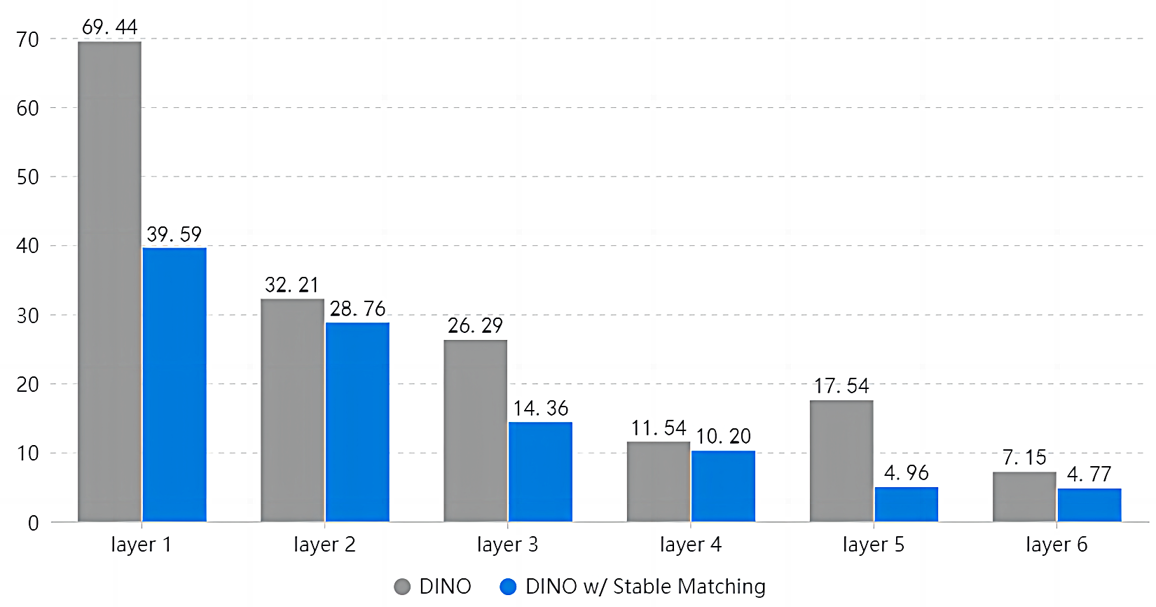
Figure 3: Comparisons of the unstable scores of DINO and DINO with stable matching.

2.4.2 Rethink the Role of Classification Scores in Detection Transformers

The new matching loss connects the DETR-like models to traditional detectors as well. Our new loss design shares a similar optimization path as traditional detectors.

An object detector has two optimization paths: one is to find a good predicted box and optimize its classification score; the other is to optimize a prediction with a high classification score to the ground truth box. Most traditional detectors assign predictions by checking their positional accuracy only. The models encourage anchor boxes that are near the ground truth. It means that most traditional detectors select the first optimization way. Differently, DETR-like matching additionally considers classification scores and uses the weighted sum of classification and localization scores as the final cost matrix. The new matching way results in conflicts between the two ways.

Since then, why still DETR-like models used classification scores during Training? We argue that it is more like a reluctant design for one-to-one matching. Previous work [40] has shown that introducing classification cost is the key to one-to-one matching. It can ensure only one positive example of the ground truth. As the localization losses (box L1 loss and GIOU loss) do not restrain negative examples, all predictions near a ground truth will be optimized toward the ground truth. There will be unstable results if only position information is considered during matching. With the classification scores in the matching, the classification scores are used as marks to denote which prediction should be used as positive examples, which can promise a stable matching during training compared with position-only matching.

However, as the classification scores are optimized independently, without any interaction with positional information, it sometimes leads the model to another optimization path, i.e., encourage the box with a larger classification score but a worse IOU score. Our position-supervised loss can help to align the classification and localization, which not only ensures a one-to-one matching, but also solves the multi-optimization problem.

With our new loss, the DETR-like models work more like traditional detectors as they both encourage predictions with larger IOU scores but a worse classification score.

2.4.3 Comparisons of Unstable Scores

To present the effectiveness of our methods. We compare the unstable scores between vanilla DINO and DINO with stable matching in Fig. 3. The unstable scores are the inconsistent matching results between adjacent decoder layers. For example, if we have $10$ ground truth boxes in an image, and only one box has a different prediction indexed matched in the $(i-1)$^th and $i$^th layers, then the unstable score of the layer $i$ is $1/10\times 100.00=10.00\%$. Typically, a model has six decoder layers. The unstable score of layer $1$ is calculated by comparing the matching results of the encoder and the first decoder layer.

We use model checkpoints at the 5000th step and evaluate models on the first 20 images in the COCO val2017 dataset. The results show that our model is more stable than DINO. There are two interesting observations in Fig. 3. First, the unstable score generally decreases from the first decoder layer to the last decoder layer, which means the higher decoder layers (with larger indexes) may have more stable predictions. Moreover, there is a strange peak in layer $5$ of DINO’s unstable scores, while DINO with stable matching does not. We suspect some randomness causes the peak.

3 Memory Fusion

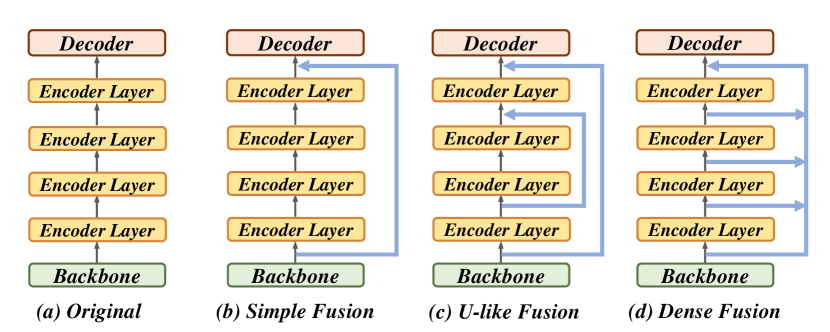
Figure 4: Comparison of our methods and baselines. We compare the (a) original memory feature with our proposed three memory fusion ways: (b) simple memory fusion, (c) U-like memory fusion, and (d) dense memory fusion.

To further enhance the model convergence speed at the early training stage. We proposed a straightforward feature fusion technique termed memory fusion, which involves merging the encoder output features at different levels with the multi-scale backbone features. We propose three different memory fusion ways, named simple fusion, U-like fusion, and dense fusion, which are shown in Fig. 4 (b), (c), and (d). For multiple features to fuse, we first concatenate them along the feature dimension and then project the concatenated feature to the original dimensions. More implementation details of memory fusion are available in Appendix Sec. B.

The dense fusion achieves better performance in our experiments, which is used as our default feature fusion. We compare the training curves of DINO and DINO with dense fusion in Fig.5. It shows that the fusion enables a faster convergence, especially in the early steps.

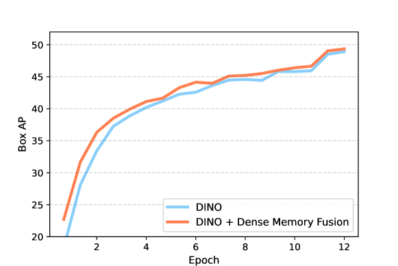
Figure 5: Comparison of the convergence speed of DINO and DINO with our dense memory fusion.

Model	Backbone	#epochs	AP	AP50	AP75	APS	APM	APL
Conditional-DETR [32]	R$50$	$108$	$43.0$	$64.0$	$45.7$	$22.7$	$46.7$	$61.5$
SAM-DETR [45]	R$50$	$50$	$39.8$	$61.8$	$41.6$	$20.5$	$43.4$	$59.6$
SAM-DETR + SMCA [45]	R$50$	$50$	$41.8$	$63.2$	$43.9$	$22.1$	$45.9$	$60.9$
Anchor-DETR [41]	R$50$	$50$	$42.1$	$63.1$	$44.9$	$22.3$	$46.2$	$60.0$
Dynamic-DETR [8]	R$50$	$12$	$42.9$	$61.0$	$46.3$	$24.6$	$44.9$	$54.4$
SMCA-DETR [14]	R$50$	$108$	$45.6$	$65.5$	$49.1$	$25.9$	$49.3$	$62.6$
AdaMixer [15]	R$50$	$36$	$47.0$	$66.0$	$51.1$	$30.1$	$50.2$	$61.8$
CF-DETR [2]	R$50$	$36$	$47.8$	$66.5$	$52.4$	$31.2$	$50.6$	$62.8$
Sparse-DETR [38]	R$50$	$50$	$46.3$	$66.0$	$50.1$	$29.0$	$49.5$	$60.8$
Efficient-DETR [43]	R$50$	$36$	$45.1$	$63.1$	$49.1$	$28.3$	$48.4$	$59.0$
BoxeR-2D [33]	R$50$	$50$	$50.0$	$67.9$	$54.7$	$30.9$	$52.8$	$62.6$
Deformable-DETR [47]	R$50$	$50$	$46.2$	$65.0$	$50.0$	$28.3$	$49.2$	$61.5$
Deformable-DETR [47]	R$50$	$50$	$46.9$	$65.6$	$51.0$	$29.6$	$50.1$	$61.6$
DAB-Deformable-DETR [28]	R$50$	$50$	$46.8$	$66.0$	$50.4$	$29.1$	$49.8$	$62.3$
DN-Deformable-DETR [22]	R$50$	$12$	$43.4$	$61.9$	$47.2$	$24.8$	$46.8$	$59.4$
DN-Deformable-DETR [22]	R$50$	$50$	$48.6$	$67.4$	$52.7$	$31.0$	$52.0$	$63.7$
$\mathcal{H}$-DETR [19]	R$50$	$12$	$48.7$	$66.4$	$52.9$	$31.2$	$51.5$	$63.5$
$\mathcal{H}$-DETR [19]	R$50$	$36$	$50.0$	$68.3$	$54.4$	$32.9$	$52.7$	$65.3$
Co-DETR [48]	R$50$	$12$	$49.5$	$67.6$	$54.3$	$32.4$	$52.7$	$63.7$
DINO-4scale [46]	R$50$	$12$	$49.0$	$66.6$	$53.5$	$32.0$	$52.3$	$63.0$
DINO-5scale [46]	R$50$	$12$	$49.4$	$66.9$	$53.8$	$32.3$	$52.5$	$63.9$
DINO-4scale [46]	R$50$	$24$	$50.4$	$68.3$	$54.8$	$33.3$	$53.7$	$64.8$
DINO-4scale [46]	R$50$	$36$	$50.9$	$\mathbf{69.0}$	$55.3$	$34.6$	$54.1$	$64.6$
gray!15 Stable-DINO-4scale (ours)	R$50$	$12$	$50.4$ (+$1.4$)	$67.4$	$55.0$	$32.9$	$54.0$	$65.5$
gray!15 Stable-DINO-5scale (ours)	R$50$	$12$	$50.5$ (+$1.1$)	$66.8$	$55.3$	$32.6$	$54.0$	$65.3$
gray!15 Stable-DINO-4scale (ours)	R$50$	$24$	$\mathbf{51.5}$ (+$1.1$)	${68.5}$	$\mathbf{56.3}$	$\mathbf{35.2}$	$\mathbf{54.7}$	$\mathbf{66.5}$

Table 2: Comparison to prior DETR variants on COCO val2017 with ResNet-50 backbones. The numbers in brackets are AP improvements compared with corresponding DINO models under the same settings.

Model	Backbone	#epochs	AP	AP50	AP75	APS	APM	APL
$\mathcal{H}$-DETR [19]	Swin-L (IN-$22$K)	$12$	$56.1$	$75.2$	$61.3$	$39.3$	$60.4$	$72.4$
$\mathcal{H}$-DETR [19]	Swin-L (IN-$22$K)	$36$	${57.6}$	${76.5}$	${63.2}$	${41.4}$	${61.7}$	${73.9}$
Co-DETR [48]	Swin-L (IN-$22$K)	$12$	${56.9}$	${75.5}$	${62.6}$	${40.1}$	${61.2}$	${73.3}$
DINO-4scale [46]	Swin-L (IN-$22$K)	$12$	$56.8$	$75.6$	$62.0$	$40.0$	$60.5$	$73.2$
DINO-4scale [46]	Swin-L (IN-$22$K)	$36$	$58.0$	$\mathbf{77.1}$	$\mathbf{66.3}$	$41.3$	$62.1$	$73.6$
gray!15 Stable-DINO-4scale (ours)	Swin-L (IN-$22$K)	$12$	${57.7}$ (+$0.9$)	$75.7$	${63.4}$	$39.8$	${62.0}$	${74.7}$
gray!15 Stable-DINO-4scale (ours)	Swin-L (IN-$22$K)	$24$	$\mathbf{58.6}$ (+$0.6$)*	$76.7$	${64.1}$	$\mathbf{41.8}$	$\mathbf{63.0}$	$\mathbf{74.7}$

Table 3: Comparison to prior DETR variants on COCO val2017 with Swin-Transformer Large backbones. * We compare our 24-epoch Stable-DINO with 36-epoch DINO here.

Model	#queries	Mask AP	Box AP	AP${}_{50}^{mask}$	AP${}_{75}^{mask}$	AP${}_{S}^{mask}$	AP${}_{M}^{mask}$	AP${}_{L}^{mask}$
Mask2Former [6]	$100$	$38.7$	$-$	$59.8$	$41.2$	$18.2$	$41.5$	$59.8$
MaskDINO [23]	$300$	$41.4$	$45.7$	$62.9$	$44.6$	$21.1$	$44.2$	$61.4$
gray!15 Stable-MaskDINO (ours)	$300$	$\mathbf{42.1}(+0.7)$	$\mathbf{47.0}(+1.3)$	$\mathbf{63.4}$	$\mathbf{45.7}$	$\mathbf{21.9}$	$\mathbf{44.5}$	$\mathbf{62.2}$

Table 4: Results of Stable-MaskDINO compared with other state-of-the-art instance segmentation models on COCO val2017. All models trained with a ResNet-50 backbone for 12 epochs.

4 Experiments

4.1 Settings

Dataset.

We conduct experiments on the COCO 2017 object detection dataset [27]. All models were trained using the train2017 set without extra data and evaluated their performance on the val2017 set. We report our results with two different backbones, including ResNet-50 [17] pretrained on ImageNet-1k [10] and Swin-L [30] pretrained on ImageNet-22k [10].

Implementation Details.

We test the effectiveness of our stable matching strategy based on DINO [46]. We trained our models on COCO training using AdamW optimizer [31, 21] with a learning rate of $1\times 10^{-4}$ for 12 epochs, and the learning rate is reduced by a factor of 0.1 at the 11^th epoch. In the case of 24-epoch settings, the learning rate is decreased at the 20^th epoch. We set the weight decay to $10^{-4}$. We conduct all our experiments based on detrex [12]. We follow their hyperparameters as default for other DETR variants. As the new loss design results in a smaller scale of classification loss, we empirically choose a $6.0$ as the classification loss weight. Moreover, we found a proper Non-Maximum Suppression (NMS) can still help the final performance for about $0.1-0.2$ AP. We use NMS by default with a threshold $0.8$. We use a random seed 60 in all our experiments to ensure the results are reproducible. DINO with the seed $60$ in detrex [12] has the same results (49.0 AP) as the original paper.

4.2 Main Results

As shown in Table 2, we firstly compare our Stable-DINO on COCO object detection val2017 set with other DETR variants with ResNet-50 [18] backbone. Stable-DINO-4scale and Stable-DINO-5scale can achieve 50.2 AP and 50.5 AP on $1\times$ scheduler, which gains $1.2$ and $1.1$ AP over the DINO-4&5 scale $1\times$ baselines. And with $2\times$ training scheduler, Stable-DINO-4scale even increased AP by $1.1$ and $0.6$ compared with DINO-4scale $2\times$ and $3\times$ baselines. Table 3 compares our models to other state-of-the-art Transformer-based detectors with large backbones, such as the ImageNet-22k [10] pre-trained Swin-Large backbone. Stable-DINO-4scale can achieve 57.7 AP on $1\times$ and obtain 58.6 AP for $2\times$ scheduler, which outperforms the DINO $1\times$ and $3\times$ baselines by 0.9 and 0.6 AP.

Comparison with SOTA methods are available in Table 10.

4.3 Generalization of our Methods

To verify the generalization of our models, we ran experiments on other DETR variants. The results are available in Table 5. Our methods show consistent improvement on existing models, including Deformable-DETR [47], DAB-Defomable-DETR [28], and $\mathcal{H}$-DETR [4].

Model	AP	APs	APm	APl
Deformable-DETR [47]	43.8	26.7	47.0	58.0
gray!15 Stable-Deformable-DETR (Ours)	45.1(+1.3)	28.6	48.8	61.3
DAB-Deformable-DETR [28]	44.2	27.5	47.1	58.6
gray!15 Stable-DAB-Deformable-DETR (Ours)	45.2(+1.0)	27.7	49.0	61.6
$\mathcal{H}$-DETR [28]	48.6	30.7	51.2	63.5
gray!15 Stable-$\mathcal{H}$-DETR (Ours)	49.2 (+0.6)	32.7	52.8	64.9

Table 5: Effectiveness of our methods on other DETR variants. All models are trained with a ResNet-50 backbone for 12 epochs. The models with the prefix “Stable” use our proposed methods.

To further present the effectiveness of our methods on different tasks, we implement our methods on MaskDINO [23] for both object detection and segmentation. We name the new model Stable-MaskDINO. Stable-MaskDINO outperforms MaskDINO on both detection and segmentation tasks, as shown in Fig. 4.

4.4 Ablation Study

We present ablations in this section. We use ResNet-50 backbones and 12-epoch training as the default setting.

Effectiveness of model designs.

We first verify the effectiveness of each design in our model. The results are available in Table 6. To make a fair comparison, we test DINO with NMS $0.8$ in row $1$ of the table. The model has $0.2$ gains compared with the default test way,

The results show that the position-supervised loss and the position-modulated cost help the final results, with +0.6 AP and +0.4 AP gains, respectively. It is worth noting that the DINO has achieved high performance already; hence each gain is hard to obtain.

We find that dense fusion works best among the three ways by comparing the different memory fusion ways. It brings $+0.2$ AP and $+0.5$ AP₅₀ compared with baselines. Moreover, the fusion helps a lot during the early training steps, as shown in Sec. 3.

Comparisons of different loss designs.

We compared the effectiveness of different loss designs in Table 7. We ignore the transformation function $\varepsilon$ (see Sec. 2.2) for simplifications in the table. To keep a fair comparison, we use loss weight as $10.0$ in all experiments in the table. All models train trained without memory fusion and position-modulated cost.

There are some interesting observations in the experiments. First, with positional metrics as supervision, the model has performance gains most of the time. The methods are robust to the function design. For example, it even works well with the $f_{1}(s)=(e^{s}-1)/(e-1)$ function. Second, the introduction of classification scores (like probabilities) will result in a performance drop in models, as shown in the lines $5$, $6$, and $7$ in Table 7. it verifies our analysis in Sec. 1 and Sec. 2.4. It also demonstrates the effectiveness of our methods design. At last, convex functions like $f_{1}(s)=s^{2}$ work better than concave functions like $f_{1}(s)=s^{0.5}$. As a special case, the concave function $\sin(s\times\pi/2)$ even results in a performance drop, since it reaches $1$ fast with the increasing of $s$.

Comparisons of different loss weights.

We test different loss weights for our position-supervised loss in this section. The results are available in Table 8. The results show that our model works well for most classification weights, e.g. from $4.0$ to $10.0$. We use the position-modulated cost and use no memory in this ablation.

Ablations for the position-modulated cost.

We compare results with different function and cost weight designs in this section. The results are available in Table 9. We choose $f_{2}(s)=s^{0.5}$ and cost weight $2.0$ by default.

Model Id	PSL	PMC	Memory Fusion	AP	AP50	AP75
0 (baseline)				49.0	66.6	53.5
1 (baseline + NMS)				49.2	66.8	54.0
2	✓			49.8	66.7	54.5
3	✓	✓		50.2	66.7	55.0
4	✓	✓	Simple Fusion	50.2	66.7	55.0
5	✓	✓	U-like Fusion	50.3	66.6	55.0
6	✓	✓	Dense Fusion	50.4	67.3	55.1
7			Dense Fusion	49.4	67.3	54.1

Table 6: Ablations for different configurations. We use “PSL” and “PMC” for the position-supervised loss (Sec. 2.2) and the position-modulated cost in matching (Sec. 2.3). For a fair comparison, we list the baseline DINO with NMS (Model Id 1). All models except model 0 are tested with a NMS.

Model Id	$f_{1}(s,p)$	AP	AP50	AP75
0 (Model 1 in Table 6)	$1$	49.2	66.8	54.0
1	$s^{0.5}$	49.3	67.5	53.7
2	$s$	49.4	67.2	54.2
3	$s^{2}$	49.6	66.8	54.5
4	$s^{3}$	49.4	65.8	54.3
5	$s^{1}p^{0.25}$	48.6	66.0	52.8
6	$s^{1}p^{1}$	26.4	32.5	28.8
7	$s^{2}p^{1}$	27.4	33.7	29.8
8	$(e^{s}-1)/(e-1)$	49.6	66.8	54.4
9	$\sin(s\times\pi/2)$	48.5	67.3	52.8

Table 7: Ablations for different loss designs for the position-supervised loss. $s$ and $p$ are used for IOU scores and classification probabilities, respectively. $f_{1}(s,p)$ is an extended function of the $f_{1}(s)$ in Eq. 3 to include classification probabilities.

Model Id	CLS Weight	AP	AP50	AP75
0	4.0	49.7	66.3	54.5
1	5.0	50.1	66.6	54.9
2 (Model 3 in Table 6)	6.0	50.2	66.7	55.0
3	8.0	49.9	66.5	54.7
4	10.0	49.6	66.5	54.5
5	20.0	48.3	65.9	52.7

Table 8: Ablations for different loss weights for the position-supervised loss. The “CLS weight” means the classification weight in final losses.

Model Id	$f_{2}(s)$	Cost Weight	AP	AP50	AP75
0 (Model 2 in Table 6)	$1$	2.0	49.8	66.7	54.5
1	$s^{0.25}$	2.0	50.0	66.7	54.9
2	$s^{0.5}$	2.0	50.2	66.7	55.0
3	$s$	2.0	49.7	65.8	54.7
4	$s^{2}$	2.0	48.8	64.7	53.7
5	$s^{0.5}$	1.0	49.6	64.6	55.0
6	$s^{0.5}$	4.0	49.6	67.4	54.0
7	$s^{0.5}$	8.0	48.8	67.1	52.7

Table 9: Ablations for different designs and cost weight for the position-modulated cost. $s$ means the IOU scores. $f_{2}(s)$ is the function defined in Eq. 2.

5 Related Work

Detection Transformer.

Detection Transformer (DETR) [3] proposed a new detector with Transformer-based heads and eliminated the dependents of head-craft modules. Although the novelty design, it suffers from slow convergence and inferior performance. Many follow-ups try to solve the problem from different perspectives. For example, some work [14, 32, 41, 28] found the importance of positional priors and propose to add more positional prior to models. DAB-DETR [28], as an example, formulated the decoder queries as dynamic anchor boxes for better results. Some work [47, 33] designed new operators to fasten model training, like deformable attention in Deformable DETR. Another line of work [22, 19, 5, 48] tried to add extra branches to the decoder. They found that auxiliary tasks can help the convergence of models. There are other explorations with traditional matching [35], model pre-train [9], and so on.

Although their great progress, the unstable matching problem across decoder layers got less attention. We analyze the reason for the unstable matching problem and propose a simple but priceless solution to the problem in this paper. The new loss and matching designs introduce marginal costs to previous work, resulting in better model performance.

Variants of Focal Loss.

Our loss design is a variant of Focal loss [26]. Although it is less focused on DETR variants, there are many works [13, 25, 1] that focus on loss improvement in classical detectors. The most related work to our solution is the task-aligned loss [13]. We have a different motivation with the task-aligned loss. We focus on the stable matching problem in DETR variants, which does not exist in traditional detectors. Moreover, although the great results of task-aligned loss in one-stage detectors, the loss cannot be used to DETR variants directly. It introduces classification scores as extra supervision, which results in performance drops in the DETR-like models with one-to-one matching, as shown in Sec. 7. The key reason for the difference is the two matching ways between traditional detectors and our solutions.

In our paper, we first analyze the phenomenon of unstable matching and point out that the key is the multi-optimization path problem. Then we show that the most crucial design to solve the problem is to use and only use positional metrics to supervise classification scores. We provide a neater and more principal solution to the unstable matching problem in DETR-like models.

6 Conclusion

We analyze the stable matching in DETR-like models and present that the root cause of the problem is the multi-optimization path problem. To solve the multi-optimization path problem, we present that the key to solving it is to use positional metrics to supervise classification scores of positive examples. We then propose a new position-supervised loss and a new position-modulated cost for DETR-like models. Moreover, we propose a dense memory fusion to enhance encoder and backbone features. We validate the effectiveness of our design on many DETR-like variants.

Limitations. Although our method shows great performance, we only verify it on DETR-like image object detection and segmentation. More explorations like 3D object detection will be left as our future work. Moreover, we focus on the classification parts in the loss and matching only, while the localization parts are preserved. Analyses for the localization parts are left as our future work as well.

Appendix A More Experiments about Stable Matching

We visualize the queries with top 30 IOU scores of DINO and Stable-DINO in Fig. 6. It shows that Stable-DINO has better alignment between IOU and probability scores.

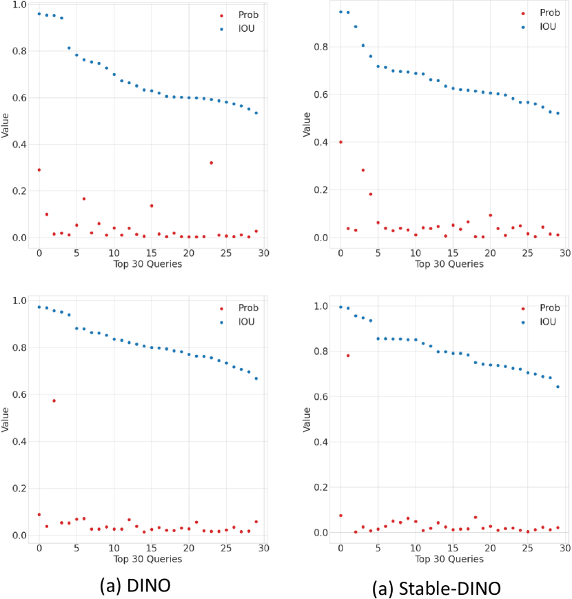
Figure 6: Comparison of top 30 queries with highest IOU values in DINO (a) and Stable-DINO (b).

Appendix B Details of Memory Fusion

The implementation of memory fusion.

The implementation of memory fusion has been depicted in Fig.7. The fusion was executed in a very simple way. The outputs from each encoder layer were amassed and subsequently concatenated with the backbone features along the channel dimension. Following concatenation, a linear projection layer, in conjunction with a norm layer, was employed to project the channel dimension, aligning it to the dimension of the decoder layer. And the fused features were then forwarded to the decoding stage.

How Memory Fusion Works?

In the DETR variants, a pre-trained backbone model is often utilized for feature extraction from the input raw images which is typically pre-trained on large-scale dataset such as ImageNet [10]. The extracted features are merged with position encodings and fed into the transformer encoder for extracting and fusing global and local information. While the encoder and backbone can be seen as the same meta-framework for feature extraction but differ in their initialization ways. The encoder’s weights are randomly initialized, whereas the backbone features are pre-trained, which means the encoder’s feature extraction capability is insufficient in the early stages of training. By fusing the pre-trained backbone features with the multi-scale features processed by the encoder, we enable the decoder to better utilize the pre-trained backbone features during the early training stages. As illustrated in Fig.5, our stable matching strategy significantly accelerates the convergence speed in the early iterations of the training process. Moreover, our newly designed dense memory fusion technique can further boost the convergence speed based on this foundation.

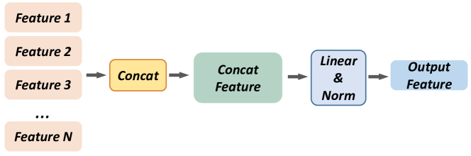
Figure 7: Detailed operation of memory fusion.

Appendix C SOTA experiments

To verify the scalability of our models, we verify our Stable-DINO with large-scale datasets and models. After pre-trained on Objects365 [39], Stable-DINO reaches $63.7$ AP on val2017 and $63.8$ AP on test-dev without test-time augmentation. We set a new SOTA with under the same setting. The results are available in Table 10.

Method	Params	Backbone Pre-training Dataset	Detection Pre-training Dataset	Use Mask	Use TTA	End-to-end	val2017 (AP)	test-dev (AP)
SwinL [30]	$284$M	IN-22K-14M	O365	✓	✓		$58.0$	$58.7$
DyHead [7]	$\geq 284$M	IN-22K-14M	Unknown*		✓		$58.4$	$60.6$
Soft Teacher+SwinL [42]	$284$M	IN-22K-14M	O365	✓	✓		$60.7$	$61.3$
GLIP [24]	$\geq 284$M	IN-22K-14M	FourODs [24],GoldG+ [24, 20]		✓		$60.8$	$61.5$
Florence-CoSwin-H[44]	$\geq 637$M	FLD-900M [44]	FLD-9M [44]		✓		$62.0$	$62.4$
SwinV2-G [29]	$3.0$B	IN-22K-ext-70M [29]	O365	✓	✓		$62.5$	$63.1$
DINO-SwinL	${218}$M	IN-22K-14M	O365		✓	✓	63.2	63.3
Stable-DINO-SwinL(Ours)	218M	IN-22K-14M	O365			✓	63.7	63.8

Table 10: Comparison of the best detection models on MS-COCO. Similar to DETR [3], we use the term “end-to-end” to indicate if a model is free from hand-crafted components like RPN and NMS. The term “TTA” means test-time augmentation. The term “use mask” means whether a model is trained with instance segmentation annotations. We use the terms “IN” and “O365” to denote the ImageNet [11] and Objects365 [39] datasets, respectively. Note that “O365” is a subset of “FourODs” and “FLD-9M”. * DyHead does not disclose the details of the datasets used for model pre-training.

Appendix D Convergence Comparison

We compare the convergence speed of Satble-DINO and DINO in Fig. 8. It shows that Stable-DINO convergence faster than DINO.

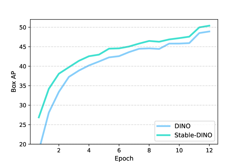
Figure 8: Convergence comparison of DINO and Stable-DINO.

Appendix E Visualizations of Encoder Sampling Points

To understand the effectiveness of memory fusion, we compare the sampling points of DINO and DINO with memory fusion in Fig. 9. We use the first checkpoint, i.e., 5000 iteration steps, during training for the visualization. As DINO use deformable attention in the Transformer encoder, we plot reference points (blue stars) and corresponding sampling points (red to yellow dots) in the figure. The results show that the memory fusion enable models to cover long range features, which introduces more global information for the model. We suspect that the encoder need to fuse global information to the features from backbones. The residual connections among encoder layers in the memory fusion accelerates the process.

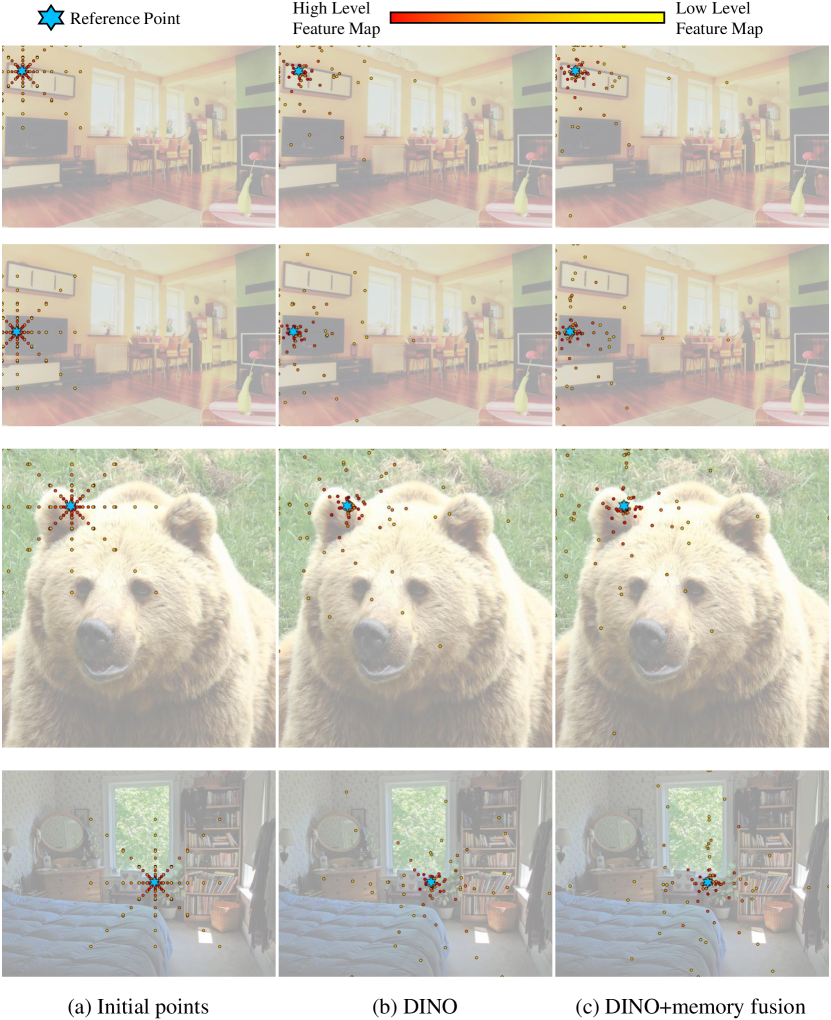
Figure 9: Comparisons of sampling points.

Appendix F Visualizations of Model Results

We visualize the results of DINO and Stable-DINO in Fig. 10. Stable-DINO has better results than DINO for its more accuracy predictions. For example, DINO has an wrong prediction “car” as shown in the first row of Fig. 10. Similarly, DINO marks the sky as a “kite” in the last row of Fig. 10, while Stable-DINO does not. It does not mean that Stable-DINO is more conservative, as it predicts the bicycles in the third row of Fig. 10. Stable-DINO has better visualization results compared with DINO.

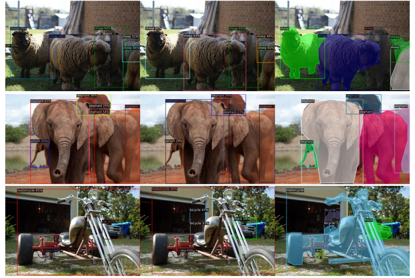
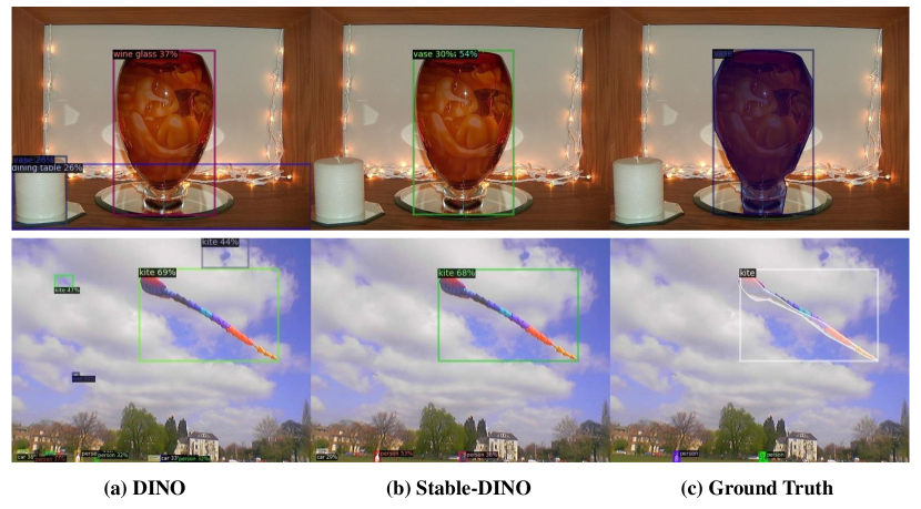
Figure 10: We compare the results of DINO (a) and Stable-DINO (b). The column (c) presents the ground truth results.

References

- [1] Nabila Abraham and Naimul Mefraz Khan. A novel focal tversky loss function with improved attention u-net for lesion segmentation. arXiv: Computer Vision and Pattern Recognition, 2018.
- [2] Xipeng Cao, Peng Yuan, Bailan Feng, Kun Niu, and Yao Zhao. Cf-detr: Coarse-to-fine transformers for end-to-end object detection. In AAAI, 2022.
- [3] Nicolas Carion, Francisco Massa, Gabriel Synnaeve, Nicolas Usunier, Alexander Kirillov, and Sergey Zagoruyko. End-to-end object detection with transformers. In European Conference on Computer Vision, pages 213–229. Springer, 2020.
- [4] Kai Chen, Jiangmiao Pang, Jiaqi Wang, Yu Xiong, Xiaoxiao Li, Shuyang Sun, Wansen Feng, Ziwei Liu, Jianping Shi, Wanli Ouyang, et al. Hybrid task cascade for instance segmentation. In Proceedings of the IEEE/CVF Conference on Computer Vision and Pattern Recognition, pages 4974–4983, 2019.
- [5] Qiang Chen, Xiaokang Chen, Jian Wang, Haocheng Feng, Junyu Han, Errui Ding, Gang Zeng, and Jingdong Wang. Group detr: Fast detr training with group-wise one-to-many assignment. 2022.
- [6] Bowen Cheng, Anwesa Choudhuri, Ishan Misra, Alexander Kirillov, Rohit Girdhar, and Alexander G. Schwing. Mask2former for video instance segmentation. 2022.
- [7] Xiyang Dai, Yinpeng Chen, Bin Xiao, Dongdong Chen, Mengchen Liu, Lu Yuan, and Lei Zhang. Dynamic head: Unifying object detection heads with attentions. In Proceedings of the IEEE/CVF Conference on Computer Vision and Pattern Recognition, pages 7373–7382, 2021.
- [8] Xiyang Dai, Yinpeng Chen, Jianwei Yang, Pengchuan Zhang, Lu Yuan, and Lei Zhang. Dynamic detr: End-to-end object detection with dynamic attention. In Proceedings of the IEEE/CVF International Conference on Computer Vision, pages 2988–2997, 2021.
- [9] Zhigang Dai, Bolun Cai, Yugeng Lin, and Junying Chen. Up-detr: Unsupervised pre-training for object detection with transformers. In Proceedings of the IEEE/CVF Conference on Computer Vision and Pattern Recognition, pages 1601–1610, 2021.
- [10] J. Deng, W. Dong, R. Socher, L.-J. Li, K. Li, and L. Fei-Fei. ImageNet: A Large-Scale Hierarchical Image Database. In Proceedings of the IEEE conference on computer vision and pattern recognition, 2009.
- [11] Jia Deng, Wei Dong, Richard Socher, Li-Jia Li, Kai Li, and Li Fei-Fei. Imagenet: A large-scale hierarchical image database. In 2009 IEEE conference on computer vision and pattern recognition, pages 248–255. Ieee, 2009.
- [12] detrex contributors. detrex: An research platform for transformer-based object detection algorithms. https://github.com/IDEA-Research/detrex, 2022.
- [13] Chengjian Feng, Yujie Zhong, Yu Gao, Matthew R. Scott, and Weilin Huang. Tood: Task-aligned one-stage object detection. International Conference on Computer Vision, 2021.
- [14] Peng Gao, Minghang Zheng, Xiaogang Wang, Jifeng Dai, and Hongsheng Li. Fast convergence of detr with spatially modulated co-attention. In ICCV, pages 3621–3630, 2021.
- [15] Ziteng Gao, Limin Wang, Bing Han, and Sheng Guo. Adamixer: A fast-converging query-based object detector. In CVPR, 2022.
- [16] Zheng Ge, Songtao Liu, Feng Wang, Zeming Li, and Jian Sun. Yolox: Exceeding yolo series in 2021. arXiv preprint arXiv:2107.08430, 2021.
- [17] Kaiming He, Xiangyu Zhang, Shaoqing Ren, and Jian Sun. Deep residual learning for image recognition. In Proceedings of the IEEE Conference on Computer Vision and Pattern Recognition (CVPR), June 2016.
- [18] Kaiming He, Xiangyu Zhang, Shaoqing Ren, and Jian Sun. Deep residual learning for image recognition. In 2016 IEEE Conference on Computer Vision and Pattern Recognition (CVPR), pages 770–778, 2016.
- [19] Ding Jia, Yuhui Yuan, † ‡ Haodi He, † Xiaopei Wu, Haojun Yu, Weihong Lin, Lei Sun, Chao Zhang, and Han Hu. Detrs with hybrid matching. 2022.
- [20] Aishwarya Kamath, Mannat Singh, Yann LeCun, Gabriel Synnaeve, Ishan Misra, and Nicolas Carion. Mdetr-modulated detection for end-to-end multi-modal understanding. In Proceedings of the IEEE/CVF International Conference on Computer Vision, pages 1780–1790, 2021.
- [21] Diederik P. Kingma and Jimmy Ba. Adam: A method for stochastic optimization. arXiv: Learning, 2014.
- [22] Feng Li, Hao Zhang, Shilong Liu, Jian Guo, Lionel M Ni, and Lei Zhang. Dn-detr: Accelerate detr training by introducing query denoising. In Proceedings of the IEEE/CVF Conference on Computer Vision and Pattern Recognition, pages 13619–13627, 2022.
- [23] Feng Li, Hao Zhang, Huaizhe xu, Shilong Liu, Lei Zhang, Lionel M. Ni, and Heung-Yeung Shum. Mask dino: Towards a unified transformer-based framework for object detection and segmentation, 2022.
- [24] Liunian Harold Li, Pengchuan Zhang, Haotian Zhang, Jianwei Yang, Chunyuan Li, Yiwu Zhong, Lijuan Wang, Lu Yuan, Lei Zhang, Jenq-Neng Hwang, et al. Grounded language-image pre-training. arXiv preprint arXiv:2112.03857, 2021.
- [25] Xiang Li, Wenhai Wang, Lijun Wu, Shuo Chen, Xiaolin Hu, Jun Li, Jinhui Tang, and Jian Yang. Generalized focal loss: Learning qualified and distributed bounding boxes for dense object detection. arXiv: Computer Vision and Pattern Recognition, 2020.
- [26] Tsung-Yi Lin, Priya Goyal, Ross Girshick, Kaiming He, and Piotr Dollár. Focal loss for dense object detection. In Proceedings of the IEEE international conference on computer vision, pages 2980–2988, 2017.
- [27] Tsung-Yi Lin, Michael Maire, Serge Belongie, James Hays, Pietro Perona, Deva Ramanan, Piotr Dollár, and C Lawrence Zitnick. Microsoft coco: Common objects in context. In European conference on computer vision, pages 740–755. Springer, 2014.
- [28] Shilong Liu, Feng Li, Hao Zhang, Xiao Yang, Xianbiao Qi, Hang Su, Jun Zhu, and Lei Zhang. DAB-DETR: Dynamic anchor boxes are better queries for DETR. In International Conference on Learning Representations, 2022.
- [29] Ze Liu, Han Hu, Yutong Lin, Zhuliang Yao, Zhenda Xie, Yixuan Wei, Jia Ning, Yue Cao, Zheng Zhang, Li Dong, et al. Swin transformer v2: Scaling up capacity and resolution. arXiv preprint arXiv:2111.09883, 2021.
- [30] Ze Liu, Yutong Lin, Yue Cao, Han Hu, Yixuan Wei, Zheng Zhang, Stephen Lin, and Baining Guo. Swin transformer: Hierarchical vision transformer using shifted windows. arXiv preprint arXiv:2103.14030, 2021.
- [31] Ilya Loshchilov and Frank Hutter. Fixing weight decay regularization in adam. 2017.
- [32] Depu Meng, Xiaokang Chen, Zejia Fan, Gang Zeng, Houqiang Li, Yuhui Yuan, Lei Sun, and Jingdong Wang. Conditional detr for fast training convergence. arXiv preprint arXiv:2108.06152, 2021.
- [33] Duy-Kien Nguyen, Jihong Ju, Olaf Booij, Martin R. Oswald, and Cees G. M. Snoek. Boxer: Box-attention for 2d and 3d transformers. arXiv preprint arXiv:2111.13087, 2021.
- [34] Duy-Kien Nguyen, Jihong Ju, Olaf Booji, Martin R. Oswald, and Cees G. M. Snoek. Boxer: Box-attention for 2d and 3d transformers. 2023.
- [35] Jeffrey Ouyang-Zhang, Jang Hyun Cho, Xingyi Zhou, and Philipp Krähenbühl. Nms strikes back. arXiv preprint arXiv:2212.06137, 2022.
- [36] Shaoqing Ren, Kaiming He, Ross Girshick, and Jian Sun. Faster R-CNN: Towards real-time object detection with region proposal networks. In C. Cortes, N. Lawrence, D. Lee, M. Sugiyama, and R. Garnett, editors, Advances in Neural Information Processing Systems (NeurIPS), volume 28. Curran Associates, Inc., 2015.
- [37] Hamid Rezatofighi, Nathan Tsoi, JunYoung Gwak, Amir Sadeghian, Ian Reid, and Silvio Savarese. Generalized intersection over union: A metric and a loss for bounding box regression. In Proceedings of the IEEE/CVF Conference on Computer Vision and Pattern Recognition, pages 658–666, 2019.
- [38] Byungseok Roh, JaeWoong Shin, Wuhyun Shin, and Saehoon Kim. Sparse detr: Efficient end-to-end object detection with learnable sparsity. arXiv preprint arXiv:2111.14330, 2021.
- [39] Shuai Shao, Zeming Li, Tianyuan Zhang, Chao Peng, Gang Yu, Xiangyu Zhang, Jing Li, and Jian Sun. Objects365: A large-scale, high-quality dataset for object detection. In Proceedings of the IEEE international conference on computer vision, pages 8430–8439, 2019.
- [40] Peize Sun, Yi Jiang, Enze Xie, Wenqi Shao, Zehuan Yuan, Changhu Wang, and Ping Luo. What makes for end-to-end object detection? arXiv: Computer Vision and Pattern Recognition, 2020.
- [41] Yingming Wang, Xiangyu Zhang, Tong Yang, and Jian Sun. Anchor detr: Query design for transformer-based detector. national conference on artificial intelligence, 2021.
- [42] Mengde Xu, Zheng Zhang, Han Hu, Jianfeng Wang, Lijuan Wang, Fangyun Wei, Xiang Bai, and Zicheng Liu. End-to-end semi-supervised object detection with soft teacher. arXiv preprint arXiv:2106.09018, 2021.
- [43] Zhuyu Yao, Jiangbo Ai, Boxun Li, and Chi Zhang. Efficient detr: Improving end-to-end object detector with dense prior. arXiv preprint arXiv:2104.01318, 2021.
- [44] Lu Yuan, Dongdong Chen, Yi-Ling Chen, Noel Codella, Xiyang Dai, Jianfeng Gao, Houdong Hu, Xuedong Huang, Boxin Li, Chunyuan Li, Ce Liu, Mengchen Liu, Zicheng Liu, Yumao Lu, Yu Shi, Lijuan Wang, Jianfeng Wang, Bin Xiao, Zhen Xiao, Jianwei Yang, Michael Zeng, Luowei Zhou, and Pengchuan Zhang. Florence: A new foundation model for computer vision. 2022.
- [45] Gongjie Zhang, Zhipeng Luo, Yingchen Yu, Kaiwen Cui, and Shijian Lu. Accelerating DETR convergence via semantic-aligned matching. In CVPR, 2022.
- [46] Hao Zhang, Feng Li, Shilong Liu, Lei Zhang, Hang Su, Jun Zhu, Lionel M. Ni, and Heung-Yeung Shum. Dino: Detr with improved denoising anchor boxes for end-to-end object detection, 2022.
- [47] Xizhou Zhu, Weijie Su, Lewei Lu, Bin Li, Xiaogang Wang, and Jifeng Dai. Deformable detr: Deformable transformers for end-to-end object detection. In ICLR 2021: The Ninth International Conference on Learning Representations, 2021.
- [48] Zhuofan Zong, Guanglu Song, and Yu Liu. Detrs with collaborative hybrid assignments training, 2022.