Machine learning one-dimensional spinless trapped fermionic systems with neural-network quantum states

Abstract

We compute the ground-state properties of fully polarized, trapped, one-dimensional fermionic systems interacting through a Gaussian potential. We use an antisymmetric artificial neural network, or neural quantum state, as an Ansatz for the wavefunction and use machine learning techniques to variationally minimize the energy of systems from two to six particles. We provide extensive benchmarks for this toy model with other many-body methods, including exact diagonalisation and the Hartree-Fock approximation. The neural quantum state provides the best energies across a wide range of interaction strengths. We find very different ground states depending on the sign of the interaction. In the nonperturbative repulsive regime, the system asymptotically reaches crystalline order. In contrast, the strongly attractive regime shows signs of bosonization. The neural quantum state continuously learns these different phases with an almost constant number of parameters and a very modest increase in computational time with the number of particles.

I Introduction

The emergence of machine learning (ML) within science has revolutionized numerous fields, from ab-initio quantum chemistry to cosmology, by directly “learning” from data to understand physical phenomena [1]. Learning algorithms based on neural networks are underpinned by universal approximation theorems (UATs), which allow for, in principle, an arbitrary accuracy of data representation. UATs are, however, existence theorems, which state that such benefits are possible, but do not necessarily indicate how such benefits are achieved [2, 3, 4, 5]. This allows for a wide range of research to build ML-based algorithms that represent physical phenomena, most notably the quantum many-body problem.

The first use of ML in a quantum many-body system was pioneered in Ref. [6] and focused on discrete systems. Since then, several different physical systems have been tackled with these techniques [7, 8, 9, 10, 11, 12, 13, 14]. Applications in quantum chemistry, like FermiNet [15, 16] or PauliNet [17, 18], have paved the way for accurate solutions of the electronic Schrödinger equation [19, 20, 21, 22, 23]. The marriage of quantum states and neural networks has lead to the novel field of neural-network quantum states (NQSs) [9].

ML-based NQS approaches solve the Schrödinger equation variationally by representing the wavefunction as a neural network [6]. NQSs are formulated so that they explicitly respect the symmetry of the many-body wave function, e.g., antisymmetry in the case of fermions. So far, there are indications that NQSs can compress the relevant information of many-body wave functions in a compact way [6, 8, 15, 16, 17, 24, 25, 26]. While NQSs come in many different setups, first-quantized, real-space formulations are often employed to perform integrals over many-particle variables, using Monte Carlo (MC) techniques. This approach essentially boils down to variational Monte Carlo (VMC) [27] with more expressible Ansätze. Moreover, the use of a ML framework allows for efficient updates of NQS parameters via automatic differentiation (AD) techniques [28]. Having direct access to the many-body wave function has the added benefit of allowing, in principle, the calculation of any many-body observable and, potentially, the simulation of many-body dynamics [6].

Our focus here is on providing a minimal implementation of a NQS for solutions of the many-body Schrödinger equation in a simple system of potential interest in condensed matter. As a proof of concept, we turn our attention to one-dimensional systems, which are computationally simpler than three-dimensional ones, and fully polarized (or spinless) fermions. We assume the fermions to be in a harmonic trap and their pair-wise interactions are characterized via a finite-range interaction. This exploratory work acts as a stepping stone towards the creation of NQSs that describe more complex nuclear systems [29, 30, 31, 32, 33].

Under certain circumstances, bosons and fermions can hold similar properties. This phenomenon is referred to as the Fermi-Bose duality and is particularly prominent in one spatial dimension settings [34, 35]. The duality manifests itself with strongly interacting fermions acting like weakly interacting bosons and vice versa [36]. Traditionally, the duality has been discussed in terms of spin-$1/2$ particles with contact interactions [37, 38]. In the case of fully polarized fermions, the Pauli exclusion principle restricts our wave function Ansatz to be antisymmetric with respect to particle position, which results in the physical effect of forbidding S-wave interactions. The corresponding interactions primarily consist of P-wave, odd parity terms [39, 36, 40, 41, 42]. We build a toy model here, which neglects some physically relevant information by utilizing an even-parity interaction, and we discuss benchmarks between several different methods to ascertain the quality of the NQS Ansatz.

Interestingly, the considered quantum many-body problem is nowadays within reach experimentally in ultracold atomic laboratories worldwide [43, 44]. Starting from the production of degenerate Fermi gases [45], experimentalists are able to tune the interactions among fermions and study the equation of state [46] and even produce few-fermion systems in a controlled way [47].

In this paper, we benchmark a minimalist implementation of the FermiNet NQS in Ref. [15] to represent one-dimensional trapped fermionic systems. In Sec. II, we define the system and the toy model Hamiltonian we consider. We provide a detailed explanation of the NQS and the benchmark many-body methods in Sec. III. A detailed analysis of the obtained results is provided in IV. We provide conclusions and an outlook of future research in Sec. V.

II System and Hamiltonian

We study a system of $A$ identical fermions with mass $m$ trapped in a harmonic trap of frequency $\omega$. We neglect spin in the following, assuming that the system is fully polarized. We focus on a finite-range Gaussian interparticle interaction, which yields the following Hamiltonian in real space:

$$\hat{H}= -\frac{\hbar^{2}}{2m}\sum_{i=1}^{A}\nabla_{i}^{2}+\frac{1}{2}m\omega^{2}\sum_{i=1}^{A}x_{i}^{2}$$

$$+\frac{V}{\sqrt{2\pi}\sigma}\sum_{i<j}\exp[-\frac{(x_{i}-x_{j})^{2}}{2\sigma^{2}}]\,.$$ (1)

The Gaussian interaction is characterized by an interaction strength, $V$, and an interaction range, $\sigma$. We choose these so that, in the limit $\sigma\to 0$ the potential becomes a contact interaction, $\to V\delta(x_{i}-x_{j})$.

We use harmonic oscillator (HO) units throughout the remainder of this work: lengths are defined in terms of $a_{\text{ho}}=\sqrt{\hbar/m\omega}$ and energies are measured in units of $\hbar\omega$. The Hamiltonian becomes

$$\hat{H}= -\frac{1}{2}\sum_{i=1}^{A}\nabla_{i}^{2}+\frac{1}{2}\sum_{i=1}^{A}x_{i}^{2}+\frac{V_{0}}{\sqrt{2\pi}\sigma_{0}}\sum_{i<j}\exp[-\frac{(x_{i}-x_{j})^{2}}{2\sigma_{0}^{2}}].$$ (2)

The interaction range is redefined, so that $\sigma_{0}=\sigma/a_{\text{ho}}\,.$ The dimensionless interaction strength $V_{0}$ is related to the dimensionful constant $V$ by $V_{0}=V/(a_{\text{ho}}\hbar\omega).$

For spinless fermions, the presence of a finite range interaction is a necessary condition to observe interaction effects. Indeed, without spin, the many-body wave function is antisymmetric on the space variables $\{x_{i},i=1,\dots,A\}$. For pairs of particles $i\neq j$, the wave function cancels whenever $x_{i}=x_{j}$. As a consequence, contact interactions do not contribute to the energy of the system. Naïvely, one expects such interaction effects to be relatively small compared with interactions of the same strength in the spinful case.

The specific choice of a Gaussian form factor for the interaction is dictated mostly by practical reasons [43, 37]. First and foremost, because of the simplicity of the associated integrals, Gaussians can be easily handled in many-body simulations, including exact diagonalization [48] as well as stochastic methods [49]. Second, as already noted above, normalized Gaussian interactions can be used to approach the contact-interaction limit by tuning the range parameter $\sigma\to 0$. Third, our ultimate goal is to simulate nuclear physics systems. Finite-range interactions are particularly relevant for nuclear physics applications, where the range of the interaction is related to the mass of meson force carriers [50]. There are examples of nuclear interactions with a Gaussian (or a sum of Gaussians) form factor, like the Gogny force [50]. We also note that Gaussian interactions have been extensively used in the analysis of several many-body systems, including the so-called “Gaussian characterization” of universal behavior [51].

Previous literature on spinless fermions has employed odd-parity interactions, which in the zero-range limit behave as $V(x)\approx\overleftarrow{\partial_{x}}\delta(x)\overrightarrow{\partial_{x}}$. This is the correct limit for the interaction of spinless fermions and it cannot be reproduced with a Gaussian potential. As such, our results should be considered as an academic toy model, and for this reason we focus on methodological benchmarks as opposed to experimental applications. We leave the study of odd parity potentials within an NQS framework for further study.

II.1 Noninteracting case

Before providing more details on how interactions are considered, we turn our attention briefly to the analytically solvable, noninteracting case. In the absence of spin, each fermion can occupy a single-particle level with energy $\epsilon_{n}=n+1/2$ characterized by a single quantum number $n$. The single-particle wavefunctions are HO eigenstates,

$$\varphi_{n}(x) =\mathcal{N}_{n}e^{-\frac{x^{2}}{2}}H_{n}\left(x\right)\,,$$ (3)

with $H_{n}(x)$ the $n$th Hermite polynomial and $\mathcal{N}_{n}=1/\sqrt{2^{n}n!\sqrt{\pi}}$, a normalization constant. The many-body wave function is a pure Slater determinant. It factorizes into an overall Gaussian envelope times a determinant involving only Hermite polynomials:

$$\Psi(x_{1},\ldots,x_{A})= \frac{1}{\sqrt{A!}}\left[\Pi_{n=0}^{A-1}\mathcal{N}_{n}e^{-\frac{x_{i}^{2}}{2}}\right]\times$$ (4)

$$\begin{vmatrix}H_{0}\left(x_{1}\right)&H_{0}\left(x_{2}\right)&\ldots&H_{0}\left(x_{A}\right)\\ H_{1}\left(x_{1}\right)&H_{1}\left(x_{2}\right)&\ldots&H_{1}\left(x_{A}\right)\\ \vdots&\vdots&\ddots&\vdots\\ H_{A-1}\left(x_{1}\right)&H_{A-1}\left(x_{2}\right)&\ldots&H_{A-1}\left(x_{A}\right)\end{vmatrix}.$$

This, in turn, may be further simplified in terms of Vandermonde determinants [37, 52].

The total energy of the many-body system is easily obtained by adding up all the occupied single-particle state energies,

$$E_{A}=\sum_{n=0}^{A-1}\epsilon_{n}=\frac{A^{2}}{2}\,,$$ (5)

and it scales with $A^{2}$. These noninteracting benchmarks are useful, especially in setting up the NQS Ansatz. In particular, as we explain below, we pretrain neural networks to the noninteracting solution. This provides an initial confined, stable and physical result from which we can start the relatively demanding variational simulations.

II.2 Density matrices

We can further characterize correlations in the system by employing many-body density matrices [53, 54]. The one-body density matrix (OBDM) for the $A$-body system is defined as the following $A-1$ integral over the many-body wave function,

$$\rho(x_{1}^{\prime},x_{1})=A\int dx_{2}\ldots dx_{A} \Psi^{*}(x_{1}^{\prime},x_{2},\ldots,x_{A})$$

$$\times \Psi(x_{1},x_{2},\ldots,x_{A}).$$ (6)

The diagonalization of $\rho$ in the space representation,

$$\int d\bar{x}\rho(x,\bar{x})\phi_{\alpha}(\bar{x}) =n_{\alpha}\phi_{\alpha}(x),$$ (7)

gives rise to the so-called natural orbitals, $\phi_{\alpha}(x)$, as well as the occupation numbers $n_{\alpha}$. $\alpha$ is a discrete index running, in principle, from $\alpha=0$ to infinity. The spectral decomposition of the OBDM allows for the following expansion:

$$\rho(x_{1}^{\prime},x_{1})=\sum_{\alpha=0}^{\infty}n_{\alpha}\phi^{*}_{\alpha}(x_{1}^{\prime})\phi_{\alpha}(x_{1}).$$ (8)

We work with a normalization such that $\sum_{\alpha}n_{\alpha}=A$.

In a noninteracting or a Hartree-Fock (HF) ground-state, one finds

$$n_{\alpha} =\begin{cases}1,\quad\alpha<A,\\ 0,\quad\alpha\geq A.\end{cases}$$ (9)

The sum in Eq. (8) is thus naturally truncated to $A$ terms. In addition, for the noninteracting case, the natural orbitals correspond to the single-particle states of Eq. (3). Performing the sum for a noninteracting system, one finds that the OBDMs have the form

$$\rho(x_{1}^{\prime},x_{1}) =\frac{e^{-\frac{x_{1}^{\prime 2}}{2}-\frac{x_{1}^{2}}{2}}}{\sqrt{\pi}}\mathcal{R}^{(A)}(x_{1}^{\prime},x_{1}),$$ (10)

where $\mathcal{R}^{(A)}(x_{1}^{\prime},x_{1})$ is a polynomial of at most order $A-1$ in both $x_{1}$ and $x_{1}^{\prime}$ [55, 56, 57].

One can also prove that a system with the occupation numbers described by Eq. (9) has a Slater determinant as a many-body wave function [58]. In other words, deviations from the uncorrelated values $n_{m}=1$ and $n_{m}=0$ provide a solid metric for intrinsic correlations in the system [42].

The two-body density matrix is also an excellent indicator of intrinsic correlations. It is usually defined as [53],

$$\Gamma(x_{1}^{\prime},x_{2}^{\prime};x_{1},x_{2})={A\choose 2}\int dx_{3}\ldots dx_{A} \Psi^{*}(x_{1}^{\prime},x_{2}^{\prime},\ldots,x_{A})$$

$$\times \Psi(x_{1},x_{2},\ldots,x_{A})\,.$$

The positive-definite diagonal elements of this matrix provide the pair correlation function (PCF) of the system,

$$g(x_{1},x_{2})=\Gamma(x_{1}^{\prime}=x_{1},x_{2}^{\prime}=x_{2};x_{1},x_{2})\,,$$ (11)

which has a direct physical interpretation in terms of the probability of finding a particle at position $x_{1}$ when another one lies at $x_{2}$ [54]. Closed expressions can be found for this object in the noninteracting case, too. In this case, the correlation function has a structure of the type

$$g(x_{1},x_{2}) =\frac{e^{-x_{1}^{2}-x_{2}^{2}}}{\pi}(x_{1}-x_{2})^{2}\mathcal{G}^{(A)}(x_{1},x_{2}),$$ (12)

where $\mathcal{G}^{(A)}(x_{1},x_{2})$ is again a polynomial of at most order $2(A-2)$ in both $x_{1}$ and $x_{2}$ [57].

III Methods

We now describe the different quantum many-body approaches that we have used to benchmark our few-body solutions. We start by providing a description of the NQS Ansatz, and then move on to describe briefly the exact diagonalization method and the Hartree-Fock approximation for the cases with $A>1$. We end the section with a description of two additional numerical methods employed to benchmark specifically the $A=2$ case.

III.1 Neural quantum states

III.1.1 Architecture

Our NQS Ansatz is a fully antisymmetric neural network, inspired by the implementation of FermiNet [15]. The input to our network are the $A$ positions of fermions in the system, $\{x_{i},i=1,\ldots,A\}$, and the output is the many-body wave function $\Psi_{\theta}(x_{1},\ldots,x_{A})$, which depends on a series of network weights and biases, succinctly summarized by a multidimensional variable $\theta$. We provide a schematic representation of the network architecture in Fig. 1. The network is composed of 4 core components: equivariant layers, generalized Slater matrices (GSMs), log-envelope functions, and a summed signed-log determinant function. We now proceed to describe each of the 4 core components of the NQS.

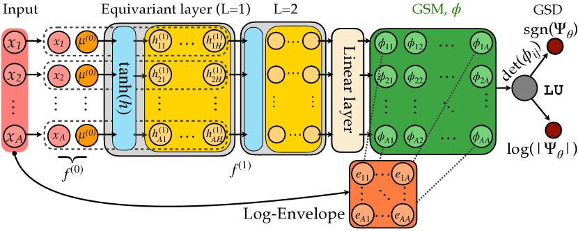
Figure 1: The NQS Ansatz of this work for $L=2$ equivariant layers of $H$ hidden nodes. The input to the network are the $\{x_{i},i=1,\ldots,A\}$ particle positions. These are processed by $2$ equivariant layers (light gray areas), to ensure that the NQS maintains equivariance throughout its forward pass. The grey dashed lines denote the row-wise application of the shared layer. Its nonlinear activation function is an hyperbolic tangent (blue area). The output of the second intermediate equivariant layer $h^{(2)}$ is passed through a shared linear layer to yield a $A\times A$ matrix $M$ which is element-wise multiplied with the log-envelope layer (orange area) thus yielding our GSM $\phi$ (green area). In a final step, a LU decomposition is used to find the sign and logarithm of the absolute value of the many-body wavefunction, $\Psi_{\theta}$.

In order for the NQS to respect antisymmetry, we enforce permutation equivariance across the network. The inputs to our network are an $A$-dimensional vector, $x\in\mathbb{R}^{A}$. The outputs of an equivariant layer, $h_{i}$, are such that any permutation of the input variables, $\pi$, permutes the outputs too, $h_{i}(x_{\pi(1)},\ldots,x_{\pi(A)})=h_{\pi(i)}(x_{1},\ldots,x_{A})$.

To ensure equivariance, we follow the methodology of Ref. [59]. We preprocess the input layer by adding a permutation-invariant feature, which in our case is the mean many-body position, $\mu^{(0)}=\frac{1}{A}\sum_{i=1}^{A}x_{i}$. The input to the first layer is then a concatenation of $x\in\mathbb{R}^{A}$, and the corresponding mean position, $\mu^{(0)}\in\mathbb{R}$. This defines an input feature $f^{(0)}\in\mathbb{R}^{A\times 2}$, such that

$$f^{(0)}_{ij}=\begin{cases}x_{i}&\text{if }j=1\\ \mu^{(0)}&\text{if }j=2\ .\end{cases}$$ (13)

The first equivariant layer $(L=1)$ of the network is shown in a grey area in Fig. 1. Each row of the input feature is passed through a shared layer to build an intermediate $H$-dimensional representation of the positions, $h^{(1)}\in\mathbb{R}^{A\times H}$ (yellow area in Fig. 1). This layer consists of a linear transformation with weights $W^{(1)}\in\mathbb{R}^{H\times 2}$ and biases $b^{(1)}\in\mathbb{R}^{1\times H}$ combined with a nonlinear activation function. We choose a hyperbolic tangent activation function, since this is continuous and differentiable, a requirement when it comes to computing many-body kinetic energies. Explicitly, each row $h^{(1)}_{i}\in\mathbb{R}^{1\times H}$ reads

$$h^{(1)}_{i}=\tanh\left(f^{(0)}_{i}W^{(1)^{\mkern-1.5mu\mathsf{T}}}+b^{(1)}\right)\ .$$ (14)

The second equivariant layer $(L=2)$ takes the output of the first layer, $h^{(1)}$, and their column-wise averages $\mu^{(1)}\in\mathbb{R}^{H}$, to define a new input feature $f^{(1)}\in\mathbb{R}^{A\times 2H}$ such that

$$f^{(1)}_{ij}=\begin{cases}h^{(1)}_{ij}&\text{if }j\leq H\\ \mu^{(1)}_{i}&\text{if }j>H\ .\end{cases}$$ (15)

Similarly to the first layer, the input feature is passed through a shared layer with weights $W^{(2)}\in\mathbb{R}^{H\times 2H}$, biases $b^{(2)}\in\mathbb{R}^{1\times H}$ and the same nonlinear activation function. A residual connection is also added so that each row of the output $h^{(2)}_{i}\in\mathbb{R}^{1\times H}$ explicitly reads

$$h^{(2)}_{i}=\tanh\left(f^{(1)}_{i}W^{(2)^{\mkern-1.5mu\mathsf{T}}}+b^{(2)}\right)+h^{(1)}_{i}\ .$$ (16)

After the second equivariant layer, $h^{(2)}$ goes through a linear layer (see beige area in Fig. 1) with shared weights $W^{(M)}\in\mathbb{R}^{A\times H}$ and biases $b^{(M)}\in\mathbb{R}^{1\times A}$ to output a matrix $M\in\mathbb{R}^{A\times A}$. Each row $M_{i}\in\mathbb{R}^{1\times A}$ reads

$$M_{i}=h^{(2)}_{i}W^{(M)^{\mkern-1.5mu\mathsf{T}}}+b^{(M)}\ .$$ (17)

At this stage, asymptotic boundaries conditions, such as the wave function decaying at infinity, are not yet incorporated. To this end, we employ an envelope function [60], implemented in the log-domain for numerical stability. The log-envelope matrix has the form

$$\ln(e_{ij})=-\left(x_{i}W^{(e)}_{j}\right)^{2},$$ (18)

where $i$ and $j$ represent the index for the particle and the orbital, respectively, and $W^{(e)}\in\mathbb{R}^{A}$ is the weight that is learned to determine the log-envelope of each orbital. We use Gaussian envelopes, instead of the exponential ones of Ref. [15], which are closer to the noninteracting solution of Eq. (4).

We then take an element-wise product of $M$ with the corresponding envelope,

$$\phi_{ij}=M_{ij}e_{ij},$$ (19)

which yields a GSM. Each element of this matrix, $\phi_{ij}=\phi_{j}(x_{i};\{x_{/i}\})$, may be understood as a generalized single-particle orbital on state $j$. This orbital does not only depend on the position of the particle $i$, but also on the positions of other particles in a permutation-invariant way, as indicated by the notation $\{x_{/i}\}$ [15]. This has the significant benefit of making all orbitals depend on all particle positions, which amounts to an efficient encoding of backflow correlations in the wavefunction [10, 15, 61], as discussed further in Sec. III.1.4.

Finally, we take the determinant of the GSM $\phi$ to obtain an antisymmetric wave function. This is generically referred to as a generalized Slater determinant (GSD). In principle, a single GSD is sufficient to represent any antisymmetric wave function [62]. Empirically, we also observe that one GSD captures nearly all the correlations in this system [30]. We note that the GSD is computed within the log-domain via a lower-upper (LU) decomposition. This choice is dictated by numerical stability.

Our computational framework is general, and we can modify both the number of equivariant layers, $L$, and the number of hidden nodes, $H$. Our NQS uses $L=2$ equivariant layers of $H=64$ hidden nodes each. This choice shows optimal results in terms of convergence according to numerical tests that can be found in Ref. [30]. Our code can also work with more than one GSM and GSDs. If we were to employ $D$ GSDs to describe the system, each determinant would have its own envelope through a $D$ dependence of the envelope weights $W^{(e)}$ in Eq. (18) [30]. In the $D>1$ case, the GSDs are summed via a signed-log-sum-exp function. We direct the reader to Appendix A of Ref. [30] for a complete and detailed explanation of the numerical implementation in the $D>1$ case.

III.1.2 Variational Monte Carlo

Having defined the NQS Ansatz, we now turn to discussing the details of how we implement a quantum many-body solution to our problem. We solve the Schrödinger equation via a VMC approach in two phases: a pretraining to an initial target wavefunction, and an energy minimization to the unknown ground-state wave function. The pre-training step can be thought of as a supervised learning exercise, where we demand that the network reproduces the many-body wave function of the noninteracting system. The idea is to obtain an initial state that is physical and somewhat similar, in terms of spatial extent, to the result after interactions are switched on. To do so, we minimize the loss,

$$\mathcal{L}^{\text{Pre}}(\theta)=\int dx_{1}\ldots dx_{A} \left|\Psi_{\theta}(x_{1},\ldots,x_{A})\right|^{2}\times$$

$$\sum_{ij}\left[\phi_{i}\left(x_{j};\{x_{/j}\}\right)-\varphi_{i}(x_{j})\right]^{2},$$

where $\phi_{i}\left(x_{j};\{x_{/j}\}\right)$ is an element of the GSM and $\varphi_{i}$ is the $i$th HO single-particle state, see Eq. (3). The loss can be reformulated via MC sampling as

$$\mathcal{L}^{\text{Pre}}(\theta)=\mathbb{E}_{X\sim\absolutevalue{\Psi_{\theta}}^{2}}\left[\sum_{ij}\left[\phi_{i}\left(x_{j};\{x_{/j}\}\right)-\varphi_{i}(x_{j})\right]^{2}\right],$$ (20)

where we define $X=(x_{1},\ldots,x_{A})$ as an $A$-dimensional random variable (or walker) distributed according to the Born probability of the many-body wavefunction, $\absolutevalue{\Psi_{\theta}}^{2}$.

Initially, a set of $N_{W}=4096$ walkers are independently distributed at the origin of configuration space using a zero-mean and unit variance $A$-dimensional Gaussian distribution. The pretraining phase is then iterated for $10^{4}$ epochs. Each epoch has three different phases. First, the $N_{W}$ walkers are distributed in proportion to the Born probability of the NQS via a Metropolis-Hastings (MH) algorithm [63, 64]. We run $10$ iterations of the MH algorithm per epoch. Second, we compute the local loss values and back-propagate to evaluate the gradients of the loss in Eq. (20) with respect to the parameters $\theta$. Third, we update the parameters using the Adam optimizer of Ref. [65], with default hyperparameters except with a learning rate of 10^-4. Once the pre-training is complete, the NQS represents an approximate solution to the noninteracting case.

The next stage of our VMC approach is to minimize the expectation value of the energy to find the ground-state wave function in a reinforcement learning setting. Using standard quantum Monte Carlo notation, the expectation value of the energy is formulated as a statistical average over local energies,

$$E(\theta) =\frac{\langle\Psi_{\theta}|\hat{H}|\Psi_{\theta}\rangle}{\langle\Psi_{\theta}|\Psi_{\theta}\rangle}=\mathbb{E}_{X\sim\absolutevalue{\Psi_{\theta}}^{2}}\left[\Psi_{\theta}(X)^{-1}\hat{H}\Psi_{\theta}(X)\right].$$ (21)

Within statistical uncertainties, this expectation value abides by the variational principle and $E(\theta)$ is larger than the ground state energy $E_{\textrm{g.s.}}$.

We compute the kinetic energy in the log domain, which leads to a local energy

$$E_{L}(X) \equiv\Psi_{\theta}(X)^{-1}\hat{H}\Psi_{\theta}(X)$$

$$=-\frac{1}{2}\sum_{i=1}^{A}\left[\left.\frac{\partial^{2}\ln\absolutevalue{\Psi_{\theta}}}{\partial x_{i}^{2}}\right|_{X}+\left.\left(\frac{\partial\ln\absolutevalue{\Psi_{\theta}}}{\partial x_{i}}\right)^{2}\right|_{X}\right]$$

$$\phantom{=}+\sum_{i=1}^{A}\frac{x_{i}^{2}}{2}+\frac{V_{0}}{\sqrt{2\pi}\sigma_{0}}\sum_{i<j}e^{-\frac{(x_{i}-x_{j})^{2}}{2\sigma_{0}^{2}}}.$$ (22)

The walkers are propagated using a MH algorithm. With this stochastic process, walkers can sample the arbitrary probability distribution dictated by the wave function Born probability. Furthermore, we follow the methodology of Ref. [19] to adapt on the fly the width of the proposal distribution in the MH sampler. The aim is to ensure that, on average, approximately $50\%$ of the walkers accept the proposed configuration at each step of the MH algorithm. This allows for the proposal distribution to effectively scale with the system size, leading to a more efficient thermalization of the Markov chain.

For the sake of numerical stability, we follow Ref. [15] and use an $\ell_{1}$ norm clipping, in which we calculate a window of “acceptable” local-energy values. We choose an $\ell_{1}$ norm as it is more robust to outliers. For a batch of local energies, we compute the local energy median, $\langle E_{L}\rangle$, with an associated $\ell_{1}$ norm deviation $\sigma_{\ell_{1}}$. The acceptable window is defined as the range $\langle E_{L}\rangle\pm 5\sigma_{\ell_{1}}$. Any values outside the window are replaced by the maximally accepted value in each side.

Once the expectation value of the energy is computed, we update the parameters of our Ansatz using its gradients with respect to $\theta$,

$$\nabla_{\theta}E(\theta)=2\mathbb{E}_{X\sim\absolutevalue{\Psi_{\theta}}^{2}}\left[\left(E_{L}(X)-E(\theta)\right)\nabla_{\theta}\ln\absolutevalue{\Psi_{\theta}(X)}\right]\ .$$ (23)

The gradient of the energy is computed by applying reverse-mode AD on the auxiliary loss function,

$$\mathcal{L}^{\text{aux}}(\theta) =2\mathbb{E}_{X\sim\bot(\absolutevalue{\Psi_{\theta}}^{2})}\left[\bot\left(E_{L}(X)-\mathbb{E}_{X\sim\absolutevalue{\Psi_{\theta}}^{2}}\left[E_{L}(X)\right]\right)\right.$$

$$\phantom{=2\mathbb{E}_{X\sim\bot(\absolutevalue{\Psi_{\theta}}^{2})}[}\left.\vphantom{\left[\bot\left(E_{L}(X)-\mathbb{E}_{X\sim\absolutevalue{\Psi_{\theta}}^{2}}\left[E_{L}(X)\right]\right)\right]}\times\ln\absolutevalue{\Psi_{\theta}(X)}\right]\,,$$ (24)

where $\bot(\ldots)$ denotes the detach function [66]. The detach function is a common ML implementation tool that allows to combine conveniently analytical calculations of gradients with an AD algorithm. When applying AD, the detach function is, by definition, equivalent to the identity function except that its derivative is equal to zero, i.e. $\bot(x)=x$ but $\partial\bot(x)/\partial x=0$. While the expectation value of Eq. (24) does not equal the energy in Eq. (21), the derivatives of both expressions with respect to the parameters of the NQS are equal. The motivation for this auxiliary loss function over the naïve implementation of Eq. (24) is numerical stability, as it allows for a calculation avoiding higher-order derivatives. One can prove that, by exploiting the detach function, the highest-ordered derivative that is required to compute the gradient is the second-order derivative with respect to $x$ for the kinetic energy. A naïve application of AD on Eq. (21) to compute the gradient of the energy would have led to a third-order mixed derivative instead.

Just as in the pretraining phase, we use $N_{W}=4096$ walkers and minimize the energy for $10^{5}$ epochs. Each epoch starts with $10$ MH sampling steps, computes the local energies through Eq. (22), and back-propagates the local gradients of Eq. (24) in order to converge the NQS towards the ground-state wave function. The parameters are updated using the Adam optimizer with default hyperparameters except with a learning rate of 10^-4 [65]. We show in Fig. 2 the evolution of the energy for one of the minimization runs, for $A=6$, $V_{0}=-20$ and $\sigma_{0}=0.5$. This represents one of the most challenging cases presented here, with a relatively large number of particles and a strong deviation from the noninteracting case. We show both the average value of $E$ (solid line) and the 99.7% confidence interval of the integral of Eq. (21). We find that in about $10000$ epochs the energy is within $0.15\%$ of the final value. The energy converges towards the ground state steadily, with relatively small oscillations around a central value (see inset of Fig. 2).

We assume that the NQS reaches the ground state after $10^{5}$ epochs and freeze the parameters $\theta$ at that stage. To compute a final estimate of the energy, we follow Ref. [67] and calculate it over multiple batches via the “blocking” method. We use $10^{4}$ batches of $4096$ walkers each, for a total of $\approx 4.1\times 10\textsuperscript{7}$ samples. We remove the aforementioned $\ell_{1}$ norm clipping, so as to not bias the final energy measurement. The final energy (and its standard deviation) is taken by averaging over these measurements. The total standard deviation is also obtained employing the blocking method of Ref. [67]. The standard deviation of an individual chain is defined as,

$$\sigma_{B}^{2} =\sigma^{2}/(L_{B}/N_{corr}),$$ (25)

with $\sigma_{B}$ and $\sigma$ being the empirical standard deviation of a block $B$ and of all samples, respectively. $L_{B}$ is the length of a given block $B$ with correlation length $N_{corr}$. This standard deviation is usually extremely small and does not affect our conclusions. All the observables throughout this paper are computed with this superset of samples, which allows for sufficiently accurate measurements. More details on the implementation of our NQS can be found in Ref. [30] as well as the GitHub repository [68].

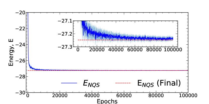
Figure 2: Convergence of the expectation value of the energy for the $A=6$ system with $V_{0}=-20$ and $\sigma_{0}=0.5$, as a function of the epoch. The NQS Ansatz is shown as a blue solid line. The 99.7% (3 standard deviations) confidence interval of the MC energy integral is shown with a shaded blue region. The final energy of the NQS, calculated via the blocking method, is shown in the red dashed line. For clarity, we show every 100^th epoch in the convergence.

III.1.3 Scaling with particle number

We now briefly comment on the scaling of the NQS method with the number of particle $A$. To asses the scaling, we estimate the memory and time requirements of the four main layers of our NQS in their forward pass. The first two layers (gray areas in Fig. 1) have, including biases, $H\times(2+1)$ and $H\times(2H+1)$ parameters, respectively. We stress that the number of parameters here is independent of the particle number. These two layers are shared and applied on $A$ row-vectors, each corresponding to a different particle, so the size of those layers is constant in $A$, while the time complexity is linear in $A$. The two remaining layers, the GSM and log-envelope layers, have, including biases, $D\times(H+1)\times A$ and $D\times A$ parameters, respectively. For these two layers, the size is linear in $A$, while the time complexity is quadratic in $A$. Lastly, the final evaluation of the determinants of the GSMs is parameter-free, but with a time complexity scaling as $D\times A^{3}$.

In practice, we have set $H=64$, $L=2$ and $D=1$ while $A$ varies from two to six. Memory-wise, the dominant cost is the storage of the intermediate layer weight matrix (quadratic in $H$) despite being constant in $A$. For example, the $A=2$ NQS has $8580$ parameters and the $A=6$ NQS has $8844$ parameters, which corresponds to a small $3\%$ increase due to the linear dependence on $A$ of the number of parameters. Regarding the computational cost, the asymptotically dominant term is the evaluation of the determinants (cubic in $A$ for the forward pass). In our simulations, however, we find that the increase of walltime per epoch with $A$ for our NQS is relatively small for the system sizes studied. In the $A=2$ case, the walltime is approximately $0.1$ s per epoch, whereas it raises to $0.3$ s per epoch in the $A=6$. This linear scaling suggests that we have not yet reached the asymptotically large $A$ behavior. Further profiling of our VMC simulations indicates that, for $A\leq 6$, the dominant contribution in terms of walltime actually comes from the MH sampling [69]. This part of the VMC algorithm is significantly more time consuming than any of the forward or backward network passes, and hence should be addressed in any time optimisation strategy. For reference, we have run all our experiments on a single P4000 Quadro GPU and overall walltime may be significantly sped up with hardware improvements.

Finally, in all the above considerations we have assumed $H$ is kept fixed while $A$ increases. The mild scaling laws that are resulting from this assumption are of course limited by the degradation of the expressivity of the network when $A$ increases. As a minimal requirement one must have $A\leq H$ to ensure the that the GSMs are full-rank and the NQS is not vanishing. To test how the expressivity of the network evolves with $A$, we have performed some additional numerical tests for the $A=12$ system with the same values of $L$ and $D$, but changing $H$. While we do not have exact benchmarks to compare with, we have found that, in this case, the NQS Ansatz still reaches an energy lower than the corresponding HF upper bound for $H>16$. The final energy values for $H=64$, $128$ and $256$ are essentially converged. We interpret this as a sign that the network expressivity can still be kept under control even if an increase of $H$ might be needed to ensure that the NQS bias remains negligible. Further explorations for larger particle numbers need to be carried out to better characterize any expressivity limits in our NQS Ansatz.

III.1.4 Backflow correlations

Our approach is different to previous ML implementations [15, 31, 32, 33], particularly FermiNet, in various ways. We drop the convolution layers, omit any accommodation of spin dependency, use Gaussian envelopes instead of exponential ones, and work with improved numerical stability on the sum of GSDs. Crucially, we also do not incorporate any explicit Jastrow factor. This does not hamper the quality of the corresponding wave function, as we shall see below.

The most relevant aspect underlying the success of our NQS implementation is its ability to incorporate backflow correlations. In the noninteracting and the HF descriptions, the many-body wave function is a Slater determinant of orbitals that depend on single-particle positions alone [60, 70, 58]. In our NQS implementation, we exploit the permutation equivariance together with a determinant layer, which introduces a form of backflow to the wavefunction representation [71, 72, 73]. This converts single-particle orbitals into quasi-particle orbitals with an extended, permutation invariant dependence on the position of all particles, and allows for a shift of the nodal surface of the NQS wave function [74]. Backflow transformations allow to incorporate correlations into the many-body wave functions. Our NQS representation, in particular, provides a flexible, numerically cheap and relatively universal representation of these correlations [10, 15], which can be efficiently learned during the VMC process.

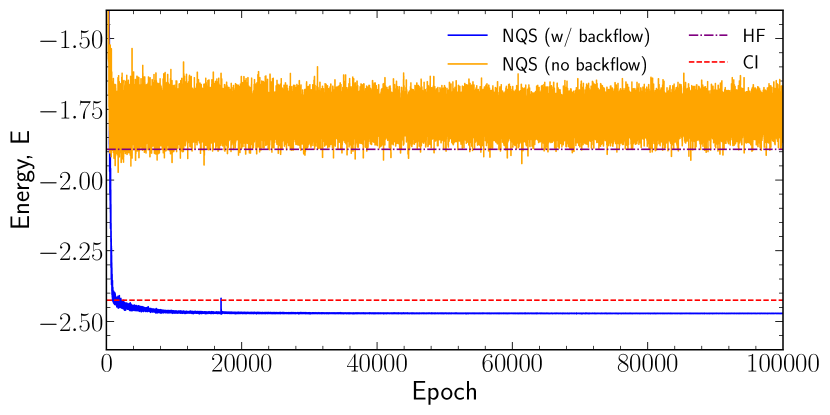
Figure 3: Convergence of the expectation value of the energy for the $A=2$ system with $V_{0}=-20$ and $\sigma_{0}=0.5$, as a function of the epoch. The standard NQS Ansatz (with backflow) is shown as a blue solid line, and overcomes the exact diagonalisation benchmark (dashed red line). An NQS Ansatz without backflow (orange line) converges to the HF solution instead.

We perform an insightful numerical experiment to clarify the importance of backflow capabilities in our NQS. The NQS Ansatz can be easily modified to remove any backflow, by eliminating the dependence on $\mu$ in the equivariant layers. This procedure roughly reduces by a half the number of parameters of the model. Moreover, in a network with a single Slater determinant and without backflow transformation, one expects the variational process to simply lead to the HF determinant. This is exactly what we observe in Fig. 3, where we show energy minimisation curves for $A=2$ particles with an interaction strength of $V_{0}=-20$ and a range $\sigma_{0}=0.5$. The figure provides results for the standard NQS architecture (with backflow, blue solid lines) and for a modified NQS without backflow (orange solid lines). The NQS without backflow reaches the Hartree-Fock energy, which is the corresponding optimal energy within a pure single-particle framework. It also shows substantial oscillations around the energy minimum. In contrast, after incorporating backflow correlations, the NQS can reach (and, in fact, outperform) a direct diagonalization benchmark with minimal oscillations. We take this as an indication that the presence of backflow in the Ansatz, which is a consequence of permutational equivariance, gives the NQS a remarkable ability to accurately represent beyond mean-field correlation between fermions. Furthermore, the statistical fluctations of the energy are mitigated with the addition of backflow, which indicates that backflow is fundamental in achieving accurate ground-state energies.

III.2 Direct diagonalisation

We have employed a direct diagonalisation (or configuration interaction) method to provide a benchmark for the $A$-body NQSs. Specifically, we use the HO as the single-particle basis. We express the Hamiltonian of Eq. (2) in second quantization,

$$\hat{H}=\sum_{\alpha=1}^{A}\epsilon_{\alpha}\hat{n}_{\alpha}+\frac{1}{2}\sum_{\alpha,\beta,\gamma,\delta}V_{\alpha\beta,\delta\gamma}\hat{a}_{\alpha}^{\dagger}\hat{a}_{\beta}^{\dagger}\hat{a}_{\gamma}\hat{a}_{\delta},$$ (26)

where $V_{\alpha\beta,\delta\gamma}$ is the matrix element in the single-particle HO basis, with an analytical expression given in Ref. [75]. $\hat{n}_{\alpha}=\hat{a}_{\alpha}^{\dagger}\hat{a}_{\alpha}$ is the number operator, and $\hat{a}_{\alpha}^{\dagger}$ ($\hat{a}_{\alpha}$) are the fermionic creation (annihilation) operators of the HO state $\alpha$.

In our implementation, we truncate the basis according to the many-body noninteracting energy, which also defines a single-particle basis truncation. We consider only the first $N_{\text{max}}=20$ single-particle HO modes for all particle numbers. This is the maximum number of states allowed by our current resources, which are limited by the precision in the calculation of the interaction matrix elements. Even with these limitations, the results of the repulsive regime are converged. In general, the convergence is slower for attractive interactions, as reported for instance in the zero-range case in Ref. [76]. Having created the many-body basis, we then construct the Hamiltonian matrix and diagonalize it using the standard Lanczos algorithm. For details of this method, please refer to Refs. [77, 48].

Our calculations are limited by the basis truncation $N_{\text{max}}$, which means that the results obtained through diagonalization are not exact and can only provide upper-bound energies. Using a larger basis would lead to better results, but the many-body basis dimension scales exponentially with the number of particles, making it impractical for large systems.

As a consequence of using the HO basis, we obtain less error in the energy calculation for the repulsive interaction regime than for an attractive interaction. As we shall see below, this can be understood in terms of the spatial rearrangement of the system. However, as the number of particles increases even without changing the single-particle basis, the accuracy of the results diminishes. In this article, we have only considered the ground state, but we stress that this method also provides predictions for excited states.

III.3 Hartree-Fock

We provide an additional benchmark by looking at the HF ground state, which is a minimal uncorrelated Ansatz for the many-body wavefunction. We solve the problem in coordinate space, in keeping with the NQS implementation. This representation is particularly useful in capturing the relatively large changes in shape of the density distribution, which may otherwise be hard to describe with fixed-basis approaches.

The HF orbitals $\phi_{\alpha}(x)$ with $\alpha=0,\ldots,A-1$ are fully occupied, with occupation numbers $n_{\alpha}=1$. All the remaining states with $\alpha\geq A$ are empty, $n_{\alpha}=0$. The HF orbitals are used to construct a one-body density matrix,

$$\rho^{\text{HF}}(x_{1}^{\prime},x_{1})=\sum_{\alpha=0}^{A-1}\phi^{*}_{\alpha}(x_{1}^{\prime})\phi_{\alpha}(x_{1}),$$ (27)

and the corresponding density profile $n^{\text{HF}}(x)=\rho^{\text{HF}}(x_{1}=x,x_{1}^{\prime}=x)$. The orbitals are obtained from the HF equations,

$$\left[-\frac{1}{2}\nabla^{2}+\frac{1}{2}x^{2}\right]\phi_{\alpha}(x)+\int d\bar{x}\Sigma(x,\bar{x})\phi_{\alpha}(\bar{x})=\varepsilon^{\text{HF}}_{\alpha}\phi_{\alpha}(x)\,.$$ (28)

In the case of a finite-range interaction, the HF equations are a set of $A$ integro-differential equations. The HF self-energy is the sum of a direct and a (non-local) exchange term,

$$\Sigma(x_{1}^{\prime},x_{1})= \delta(x_{1}-x_{1}^{\prime})\int dx\,V(x_{1}-x)n^{\text{HF}}(x)$$

$$+V(x_{1}^{\prime}-x_{1})\rho^{\text{HF}}(x_{1}^{\prime},x_{1})\,.$$ (29)

The corresponding HF energy is computed from the sum of single-particle energies and, as a consistency check, it can also be obtained from the direct integral of the mean-field, with the associated antisymmetry corrections [78].

We solve this set of self-consistent equations by iteration on a discretized mesh of equidistant points. The kinetic term is represented as a matrix using the Fourier grid Hamiltonian method [79], which works so long as the mesh extends well beyond the support of the wave functions. The mean-field can be computed efficiently with matrix operations, and Eq. (28) is reduced to an eigenvalue problem. We typically employ $N=200$ grid points extending from $x=-5$ to $5$ for small systems. For systems with $A>4$, which have larger sizes, the mesh limits are extended to $\pm 6$ and we choose $N=240$ points to keep the same mesh spacing. A computational notebook for the solution of the HF equations is available in Ref. [80].

III.4 Real-space solution for $A=2$

In the following section, we use the $A=2$ system to determine which values of interaction strength and range are interesting. We have exploited two more numerical methods to solve specifically this problem.

For $A=2$ particles, the Hamiltonian in Eq. (1) is particularly easy to handle. Following Refs. [81, 41], we introduce a center of mass (CoM), $R=\frac{1}{\sqrt{2}}(x_{1}+x_{2})$, and relative coordinate, $r=\frac{1}{\sqrt{2}}(x_{1}-x_{2})$. With these, the Hamiltonian $\hat{H}=\hat{H}_{\text{CM}}+\hat{H}_{\text{rel}}$ separates into two commuting components,

$$\hat{H}_{\text{CM}} =-\frac{1}{2}\nabla_{R}^{2}+\frac{1}{2}R^{2},$$ (30)

$$\hat{H}_{\text{r}} =-\frac{1}{2}\nabla_{r}^{2}+\frac{1}{2}r^{2}+\frac{V_{0}}{\sqrt{2\pi}\sigma_{0}}e^{-\frac{r^{2}}{\sigma_{0}^{2}}}\,.$$ (31)

The center-of-mass component is just an HO. The relative Hamiltonian includes an HO as well as the Gaussian interaction component. We note that the Gaussian form factor in relative coordinates has a different width and it is effectively wider than the original interaction.

The CoM and relative Hamiltonians can be diagonalized separately, providing eigenstates $\varphi_{\alpha}(R)$ and $\psi_{\beta}(r)$ with eigenenergies $\epsilon_{\alpha}$ and $\varepsilon_{\beta}$, respectively. For the relative coordinate, we need to solve the eigenvalue problem

$$\left[-\frac{1}{2}\nabla_{r}^{2}+\frac{1}{2}r^{2}+\frac{V_{0}}{\sqrt{2\pi}\sigma_{0}}\exp(-\frac{r^{2}}{\sigma_{0}^{2}})\right]\psi_{\beta}(r)=\varepsilon_{\beta}\psi_{\beta}(r)\,.$$ (32)

Because of the Pauli principle, the only acceptable solutions are those that are antisymmetric in the relative coordinate, $\psi_{\beta}(-r)=-\psi_{\beta}(r)$. These correspond to odd values of $\beta$, and hence the ground state will necessarily correspond to $\beta=1$ rather than lowest-energy, space-symmetric $\beta=0$ state. To solve this problem numerically, we discretize the relative coordinate in an evenly spaced mesh. As in the HF case, the kinetic term is discretized as a matrix using the Fourier grid Hamiltonian method [79]. We employ $N=200$ grid points extending from $r=-5$ to $5$. A computational notebook for this problem is also available in Ref. [80].

If a numerical solution to $\psi_{\beta}$ is available, the total two-body wavefunction is the product,

$$\Psi_{\alpha,\beta}(x_{1},x_{2})=\varphi_{\alpha}\left(\frac{1}{\sqrt{2}}(x_{1}+x_{2})\right)\times\psi_{\beta}\left(\frac{1}{\sqrt{2}}(x_{1}-x_{2})\right).$$ (33)

The total energy of the ground state is given by $E=\epsilon_{0}+\varepsilon_{1}=\frac{1}{2}+\varepsilon_{1}$. We only discuss the ground state of the system, but note that this method can also provide the rest of the spectrum for $A=2$.

III.5 Perturbation theory for $A=2$

Alternatively, one can solve for the energy $\varepsilon_{\beta}$ in Eq. (32) using standard perturbation theory tools. We take the HO as a reference state, so that $\psi_{\alpha}^{(0)}=\varphi_{\alpha}$ and $\varepsilon_{\alpha}^{(0)}=\epsilon_{\alpha}$, where $\varphi_{\alpha}$ and $\epsilon_{\alpha}$ are HO eigenstates and eigenvalues. The Gaussian interaction term is then treated as a perturbation. We employ known analytical expressions for the matrix elements $V_{\alpha\beta}=\frac{V_{0}}{\sqrt{2\pi}\sigma_{0}}\Braket{\varphi_{\alpha}}{e^{-\frac{r^{2}}{\sigma_{0}^{2}}}}{\varphi_{\beta}}$ [82]. The zero-order results are just the eigenvalues of the noninteracting confined two-particle system, Eq. (5), which in the ground state yields $E^{(0)}=2$. Noting that antisymmetry constraints force $\alpha$ and $\beta$ to take odd values, we find that the first-order perturbation theory (PT1) expression for the total energy is,

$$E^{(1)}=E^{(0)}+V_{11}=2+\frac{V_{0}}{\sqrt{2\pi}}\frac{\sigma_{0}^{2}}{(1+\sigma_{0}^{2})^{3/2}}.$$ (34)

As expected, this expression is linear in the perturbation strength $V_{0}$. The slope of the energy dependence on $V_{0}$ is dictated by $\sigma_{0}$. For small values of $\sigma_{0}$, the slope grows quadratically. In other words, the departure from the noninteracting case is quadratic in $\sigma_{0}$. For large values of $\sigma_{0}$, in contrast, the slope decreases like $1/\sigma_{0}$. This is to be expected since, by construction, the parametrization of our interaction term has such a $1/\sigma_{0}$ dependence.

Second (PT2) and third (PT3) order perturbation theory results can be readily obtained from the corresponding matrix elements $V_{\alpha\beta}$. We use up to eight additional states in the intermediate sums, which are already converged for all practical purposes. We provide a computational notebook in Ref. [80]. As we shall see below, these PT estimates allow us to find regions of parameter space where nonperturbative effects are particularly important.

IV Results

In this section, we show the results obtained for spinless fermionic systems from $A=2$ to $A=6$ with different methods. We start with a discussion of the two-body case in the first subsection. This allows us to perform an exploration of the dependence of the results in $V_{0}$ and $\sigma_{0}$. Results for $A>2$ are discussed in the following subsection, Sec. IV.2.

IV.1 Two-body sector

The two-body case in our Gaussian toy model is already relatively complicated. The solution for a zero-range interaction is well known [81], and semianalytic solutions for specific finite-range interactions are also available [41].

IV.1.1 Energy

The dependence on $V_{0}$ and $\sigma_{0}$ of the energy of the $A=2$ mimics that of heavier systems. We are particularly interested in finding regions of nonperturbative behaviour, to test the performance of the NQS Ansatz in the most challenging scenarios. We start by looking at the dependence on the range of the interaction, $\sigma_{0}$. We note that our pursuit here is mostly theoretical and that the values of interaction range and strength that we explore may not be directly accessible by near-term experiments.

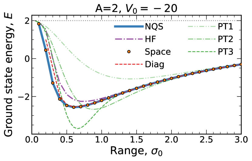
Figure 4: The ground state energy of the $A=2$ system as a function of the range, $\sigma_{0}$, for a large and attractive interaction strength, $V_{0}=-20$. The NQS Ansatz energy for $H=64$, $L=2$, and $D=1$ is shown as a solid line. The orange circles represent the real-space solution. The short-dash-dotted purple line is the Hartree-Fock solution. The double-dotted-dashed, dotted-dashed, and dashed green lines show the perturbation theory results to first (PT1), second (PT2), and third orders (PT3), respectively. The horizontal dotted line is the noninteracting energy baseline.

We start by considering a very attractive interaction, with $V_{0}=-20$. The results for the ground-state energy are shown in Fig. 4. In this plot, we show the NQS Ansatz with a solid line, which includes the statistical VMC uncertainty that is typically smaller than $10^{-5}$ in the same units. We also show the exact diagonalization (dashed line), HF (short-dashed-dotted purple line) and the real-space (filled circles) solutions. To analyze how perturbative the results are, we also display the PT1, PT2 and PT3 predictions for the energy with different linestyles.

For $A=2$ particles, the noninteracting case corresponds to $E=2$, shown in the figure as a horizontal dotted line. As expected, all the methods agree with this value as the range tends to zero, $\sigma_{0}\to 0$. As a function of the range, all energy predictions subsequently decrease, reach a model-dependent minimum value and eventually increase to reach an asymptotic $\sigma_{0}^{-1}$ behaviour.

The comparison between different methods provides an insight on the complexity of the problem. First, we note that the NQS solution agrees perfectly well with the real-space solution along a wide range of values. Second, the minimum of energy as a function of $\sigma_{0}$ lies around $\sigma_{0}\approx 0.5$ and yields $E\approx-2$ for this particular value of $V_{0}$. We conclude that the network is performing well across a wide range of values of $\sigma_{0}$.

The NQS outperforms variationally the exact diagonalization and HF solutions across a wide range of values. In particular, the HF solution has a somewhat shallower minimum at a larger value of $\sigma_{0}$. Note that the HF prediction is the optimal solution for a Slater determinant formed of single-particle orbitals, $\phi_{\alpha}(x)$ [60, 70, 58]. The HF single-particle orbitals depend on a single position. The NQS outperforms this solution by exploiting backflow correlation in the generalized orbitals of the GSM, as explained in Subsection III.1.4. The NQS prediction is also better than the exact diagonalization results at very small values of $\sigma_{0}$, where the truncated basis may have difficulties capturing the very narrow structures appearing in the $\sigma_{0}\to 0$ limit.

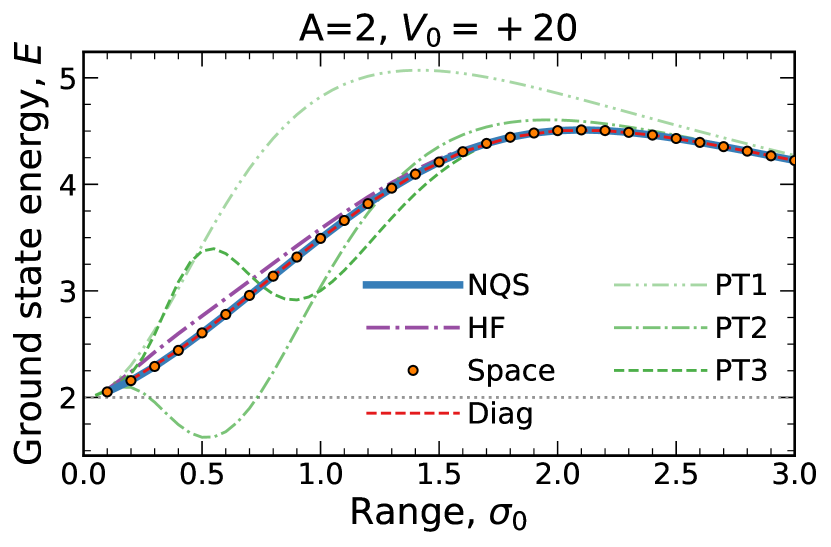
Figure 5: The same as Fig. 4 but for a large and repulsive interaction strength, $V_{0}=+20$.

The convergence of the perturbation theory results provides an indication of the “perturbativeness” of the two-body problem. The PT1 (dashed-double-dotted line) result of Eq. (34) is far too repulsive across all values of the range. It only gets close to the NQS and real-space results well beyond its shallow minimum, which happens at $\sigma_{0}=\sqrt{2}$. The PT2 results for small values of $\sigma_{0}$ are substantially closer to the NQS ones, but they cannot reproduce the correct dependence with $\sigma_{0}$ below about $\sigma_{0}\approx 2$. In contrast to the PT1 prediction, the PT2 result is more attractive than the NQS prediction beyond about $\sigma_{0}\approx 0.7$. Something similar happens with PT3, which is well below the NQS solution from $\sigma_{0}\approx 0.5$ onwards. We find that these third-order results are still rather far from the true values and, in particular, the convergence pattern is relatively erratic for $\sigma\in[0.5,0.9]$. This challenging region in parameter space may be a good test bed for the NQS solution.

We confirm that this region of ranges is particularly nonperturbative by looking at a very repulsive case. We show in Fig. 5 the predictions for the ground state energy of the $A=2$ system for a value of $V_{0}=+20$. The shape of the energy predictions here is substantially different. The NQS energy departs from the noninteracting baseline at $\sigma_{0}=0$, and increases to a maximum of around $E\approx 4$ at $\sigma_{0}=2$. Just as in the attractive case, large values of the range lead to relatively perturbative results, in the sense that PT1, PT2 and PT3 predictions agree with the exact benchmarks. In contrast, for values of the range below $\sigma_{0}=1$, the PT predictions follow a complex pattern. In particular, the PT2 and PT3 results show anomalous oscillations around $\sigma_{0}=0.5$. All in all, we conclude that for values of interaction strength of the order of $V_{0}\approx\pm 20$, nonperturbative behavior occurs for interaction ranges of the order of $\sigma_{0}=0.5$. While we do not show them for brevity here, we stress that the dependence of the NQS and HF energies on the range $\sigma_{0}$ for systems with $A>2$ has a behavior very similar to those shown in Figs. 4 and 5. The interested reader can find this information in Ref. [30].

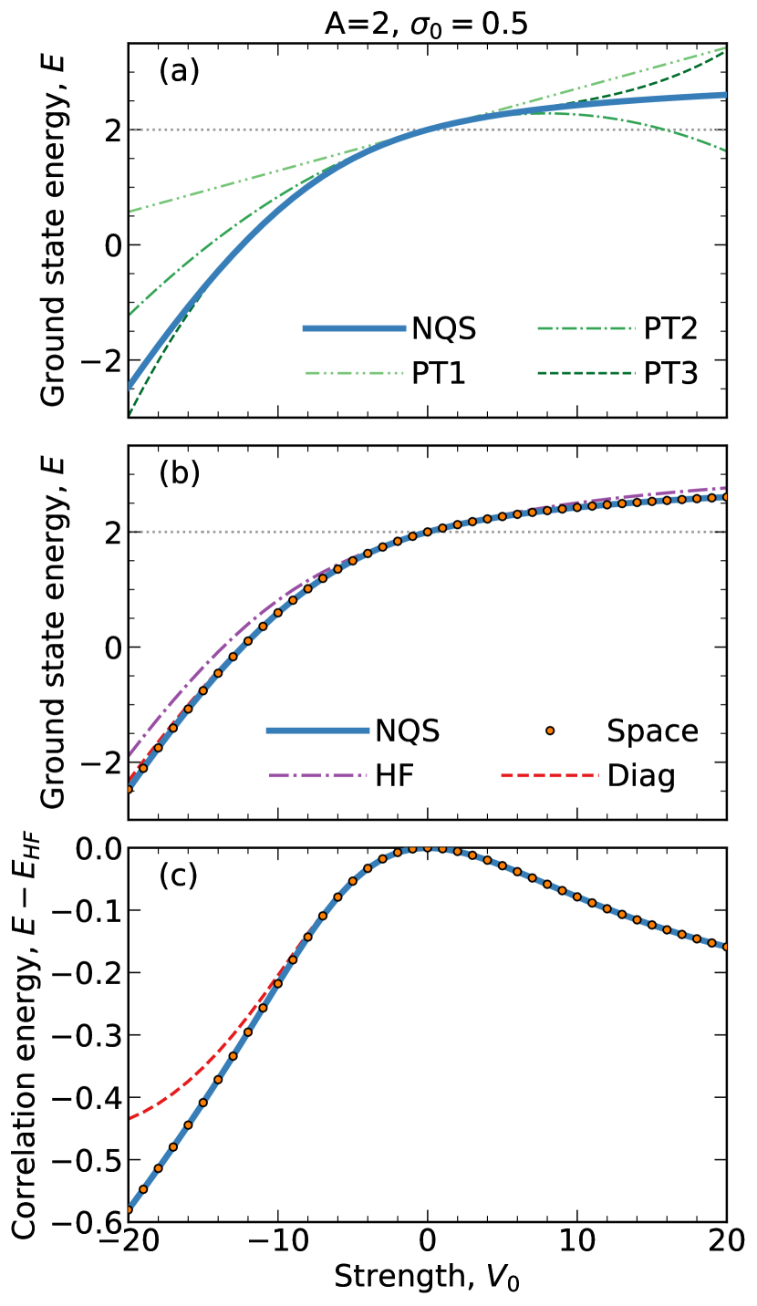
Figure 6: Energy of the $A=2$ system as a function of interaction strength, $V_{0}$, for a fixed range, $\sigma_{0}=0.5$. Panel (a): comparison of the NQS ground state energy (solid line) to perturbation theory results. Panel (b): comparison of the NQS ground state energy (solid line) to the real-space solution of the $A=2$ system (filled circles); direct diagonalisation results (dashed red line); and the HF approximation (short-dashed-dotted purple line). Panel (c): NQS, real-space solution and direct diagonalisation predictions for the correlation energy, $E_{c}=E-E_{\textrm{HF}}$.

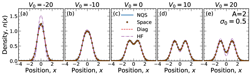
Figure 7: The density profile $n(x)$ of the $A=2$ system as a function of position $x$. Panels (a) to (e) show results for values of $V_{0}$ from $-20$ to $20$ in steps of $10$. See Fig. 6 for an explanation of the legend.

The analysis of the $\sigma_{0}$ dependence of our results leads us to conclude that a value of $\sigma_{0}=0.5$ is well within the nonperturbative regime. We now explore the dependence of the ground-state energy on the interaction strength $V_{0}$ to analyze the performance of the NQS Ansatz. The results for $A=2$ are shown in the three panels of Fig. 6. Figure 6(a) shows a comparison between the NQS ground state energy (solid lines) and the different PT results. This provides an idea of the perturbative nature of the system as a function of $V_{0}$, rather than $\sigma_{0}$. The PT1 prediction (dashed-double-dotted line) of Eq. (34) is, as expected, linear in $V_{0}$ and captures the full dependence on $V_{0}$ only for small values of $V_{0}$, $|V_{0}|<4$. PT2 results (dashed-dotted line) are valid in a wider strength range, but overpredict (underpredict) the true ground-state energy at large negative (positive) values of $V_{0}$. PT3 results (short-dashed line) work well within a range $-15<V_{0}<10$, but fail beyond this range. Again, this analysis indicates that the most attractive and repulsive values of $V_{0}$ are in a nonperturbative regime.

We compare the NQS results to more realistic benchmarks in Fig. 6(b). Overall, we find an excellent agreement between the real-space solution and the NQS prediction. The direct diagonalization result also provides a good energy prediction, although minor deviations with respect to the NQS are observed at large negative values of the coupling. The NQS provides better variational results than the HF approximation thanks to backflow correlations.

We now comment on the overall dependence of the energy on $V_{0}$. In the noninteracting limit $V_{0}=0$, all methods agree exactly with the baseline value, $E=2$. In the repulsive side, as the interaction strength increases in magnitude, the energy generally increases above the baseline, and seems to saturate to a value that lies close to $E\approx 2.5$. On the attractive side, in contrast, the energy decreases relatively rapidly. At around $V_{0}\approx-10$, the system energy becomes attractive. The total energy then decreases in absolute value as $V_{0}$ becomes more and more attractive. It is immediately clear from the energetics of the system that the attractive and the repulsive regimes are very different from each other.

This difference becomes even more evident in Fig. 6(c), which shows the correlation energy $E_{c}$ of the system. We follow textbook conventions [60] and define $E_{c}$ as the difference in ground-state energy of a given method and the HF prediction, $E_{c}=E-E_{\text{HF}}$. We note that this may not be a very insightful quantity at the two-body level, since the HF prediction is not expected to work well in the $A=2$ sector.

The correlation energy departs from zero at $V_{0}=0$. In the repulsive side, $E_{c}$ slowly increases in absolute magnitude. At $V_{0}=20$, we find $E_{c}\approx-0.15$, which is about $6\%$ of the total energy. In contrast, in the attractive regime, the NQS prediction is $E_{c}\approx-0.6$, which is a substantial contribution to the total energy of $E\approx-2$ at that same value. There is no sign of saturation of the correlation energy in either side of $V_{0}$. We also note that the direct diagonalization result departs from both the real-space and the NQS prediction for values of $V_{0}<-10$. This discrepancy is due to the truncation of the model space, as we shall see next.

IV.1.2 Density profile

To further understand the origin of the correlations of the system, we look at the density profile of the system, $n(x)$. Figure 7 shows the density profile obtained with the different many-body approaches for five different values of $V_{0}$, ranging from $-20$ to $20$ in steps of $10$. Figure 7(c) shows the noninteracting result, $V_{0}=0$. Here, all methods agree, as expected. The density profile has a well-understood dip at the center, due to the interplay between the $\alpha=0$ and $\alpha=1$ HO orbitals. These density modulations are typical in fermion systems [41]. Figures 7(d) and  7(e) show the same densities in the repulsive regime, at interaction values of $V_{0}=10$ and $20$, respectively. We find that the central dip of the density decreases, while the overall size of the density profile is relatively constant. We find a very clear agreement between the real space solution of the $A=2$ problem, the direct diagonalization method and the NQS prediction. In contrast, the HF result seems to overestimate the fermionic structures, with a lower dip and higher density maxima. In other words, the HF orbitals appear to be more localized than their correlated counterparts. A similar difference in the localization patterns of HF and fully correlated predictions was observed in the 3D Wigner crystal of an electron gas [83].

Physically, the picture that arises in the repulsive regime is akin to that of localization or (Wigner) crystallization [84, 85, 86, 87, 88, 89, 23]. As the interparticle interaction strength increases, the system minimizes the interaction energy by keeping particles beyond the interaction range. Doing so, however, may come at the price of increasing the potential energy if particles were moved away from the center of the HO well. Instead, the system prefers to localize orbitals more strongly in a periodic structure, reducing the inter-particle density in the intermediate throughs.

In contrast, the density profile in the attractive regime, shown in Figs. 7(a) and  7(b), is characterized by a relatively featureless structure. The fermionic dip disappears around $V_{0}\approx-10$ and, for more attractive strength values, the density profile is a simple peak that narrows down and increases in height as $V_{0}$ becomes more negative. In fact, a longstanding prediction in one-dimensional systems suggests that spinless fermionic systems with strongly attractive interactions should behave like noninteracting bosonic systems [39, 90, 36, 40, 35, 91, 92, 41, 42]. The density profile for the $A=2$ system clearly supports this hypothesis. It is worth stressing that the NQS grasps the bosonization transition without any further adjustments. We also stress that our results are qualitatively similar to the semi-analytical solution of Ref. [41], where a soft-core, square-well interaction was used.

Overall, the density profile of the system is extremely useful because it provides direct evidence of two very different phases of the toy model. The attractive regime shows signs of a bosonic nature in the density of the system, a prediction that bodes well with previous studies employing odd-symmetry interaction potentials [39, 90, 36, 40, 35, 91, 92, 42]. Very few predictions exist for parity-even potentials [41, 55], but the agreement between our different benchmarks in the bosonic phase indicates that the picture is relatively robust. A previous theoretical study employing an even-parity soft-core potential in the $A=2$ case [41] identified similar features in the repulsive phase. There, particles tend to localize beyond the interaction range, to move away from the repulsive core and thus minimize the energy. In fact, for repulsive interactions, the same study indicates that the localized phase is identical for both fermions and bosons [41]. All in all, the existing evidence at the two-body level for an even-parity potential indicates that there are signs of fermion-boson duality both in the attractive and the repulsive regimes.

IV.1.3 Occupation numbers

The density profile $n(x)$ is just a component of the OBDM. We can access the OBDM with the benchmark methods discussed so far. With NQSs, we calculate $\rho(x_{1}^{\prime},x_{1})$ stochastically using the ghost-particle method of Ref. [93]. For the real-space solution, we perform the integral in Eq. (6) over the uniform mesh grid. The solution of Eq. (7) can then be easily obtained as a matrix diagonalization problem in a spatially uniform grid. With the direct diagonalization method, we calculate $\rho$ in the second-quantization formalism, with the definition

$$\rho_{\alpha\beta}=\langle\Psi|\hat{a}_{\alpha}^{\dagger}\hat{a}_{\beta}|\Psi\rangle\,,$$ (35)

where $|\Psi\rangle$ is the precomputed ground-state wave function and $\rho_{\alpha\beta}$ are the matrix elements of the OBDM, $\rho$. Finally, we diagonalize $\rho$ to obtain the eigenvalues $n_{\alpha}$ in the many-body basis.

Figure 8(a) shows the evolution of the occupation numbers for the $A=2$ system as a function of interaction strength. We benchmark the NQS results (solid circles) to the real-space solution (empty circles) and the direct diagonalization approach (solid lines). We find an excellent agreement between all three methods. We note that we do not include a comparison to the HF benchmark, which provides a relatively good description of the energy of the system. For occupation numbers, however, the HF approach is limited to either fully occupied or fully unoccupied states and it cannot capture deviations in the occupation numbers from the noninteracting case.

For $A=2$, there is a double degeneracy in the natural orbital occupations, which the NQS can handle seamlessly. The hole occupation values $n_{\alpha<A}$ depart from $1$ as the absolute value of $V_{0}$ increases. We find that the rate of change is different depending on whether we are on the attractive or the repulsive side, a result that mimics the correlation energy displayed in Fig. 6(c). In the repulsive side, for $V_{0}=20$, the occupation is about $\approx 96\%$, indicating a relatively uncorrelated system. The tendency to deviate from $1$ as $V_{0}$ increases, however, indicates that even in the crystalline phase, particles are not entirely described by locally confined individual orbitals [41]. In contrast, in the attractive case, for $V_{0}\approx-20$ the occupation number is $n_{\alpha}\approx 0.9$. This suggests a stronger role of correlations in the bosonized phase.

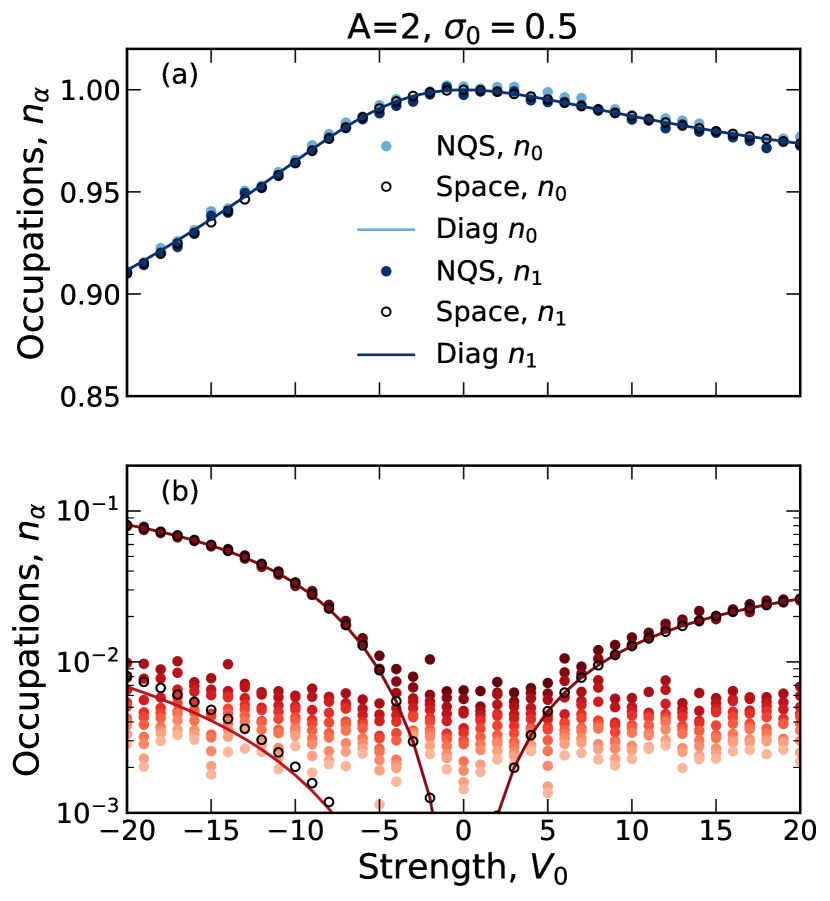
Figure 8: Occupation probabilities for the $A=2$ system as a function of interaction strength for a fixed range $\sigma_{0}=0.5$. Panel (a) shows the occupations for the two hole states below the Fermi surface. Panel (b) shows (in logarithmic scale) the occupations of particle states. We compare the NQS results (solid circles) to real space results (empty circles). Solid lines correspond to the direct diagonalisation results.

Figure 8(b) shows a similar figure for “unoccupied” orbitals, $n_{\alpha\geq A}$. The plot is given in logarithmic scale and includes the first $14$ orbitals in the NQS diagonalization. Due to the stochastic nature of the OBDM estimation in the NQS approach, there is a prominent statistical noise floor of the order of $\approx 10^{-2}$. While this limits some of the conclusions that can be drawn, we stress that the NQS many-body wave function is comparable (if not better) variationally than the other estimates. The values of $n_{\alpha}$ above the statistical threshold should therefore provide a more faithful representation of the true occupation numbers.

Just as in Fig.8(a), we find that the repulsive and attractive sides are qualitatively different. On the repulsive regime, we only see one doubly-degenerate particle state with an occupation larger than $10^{-3}$, that reaches values close to $n_{\alpha}\approx 0.02-0.03$ for $V_{0}=20$. In the attractive regime, in contrast, we find two doubly-degenerate states with occupations above $10^{-3}$. The more populated states here reach values $n_{\alpha}\approx 0.08$ for $V_{0}=-20$. The second doubly-degenerate state is observed as a prediction of the exact diagonalization and real-space solutions. It has an occupation which is roughly $10$ times smaller than the most occupied state. The NQS cannot resolve this occupation, as it lies within its statistical floor. Overall, however, the picture reinforces the idea that correlations have a very different nature on the attractive and the repulsive side. A priori, it appears that the bosonized phase has a more complex structure, admixing more single-particle modes than the corresponding crystalline phase.

IV.2 Few-body sector

We now turn our discussion to the results obtained in the few-body sector, for systems with $A=3$ up to $A=6$ particles. We continue to benchmark NQS results against the direct diagonalization approach as well as the HF method. The real-space solution is not available for $A>2$. We advance that several of the physics conclusions we drew on the two-body system remain the same in the few-body domain.

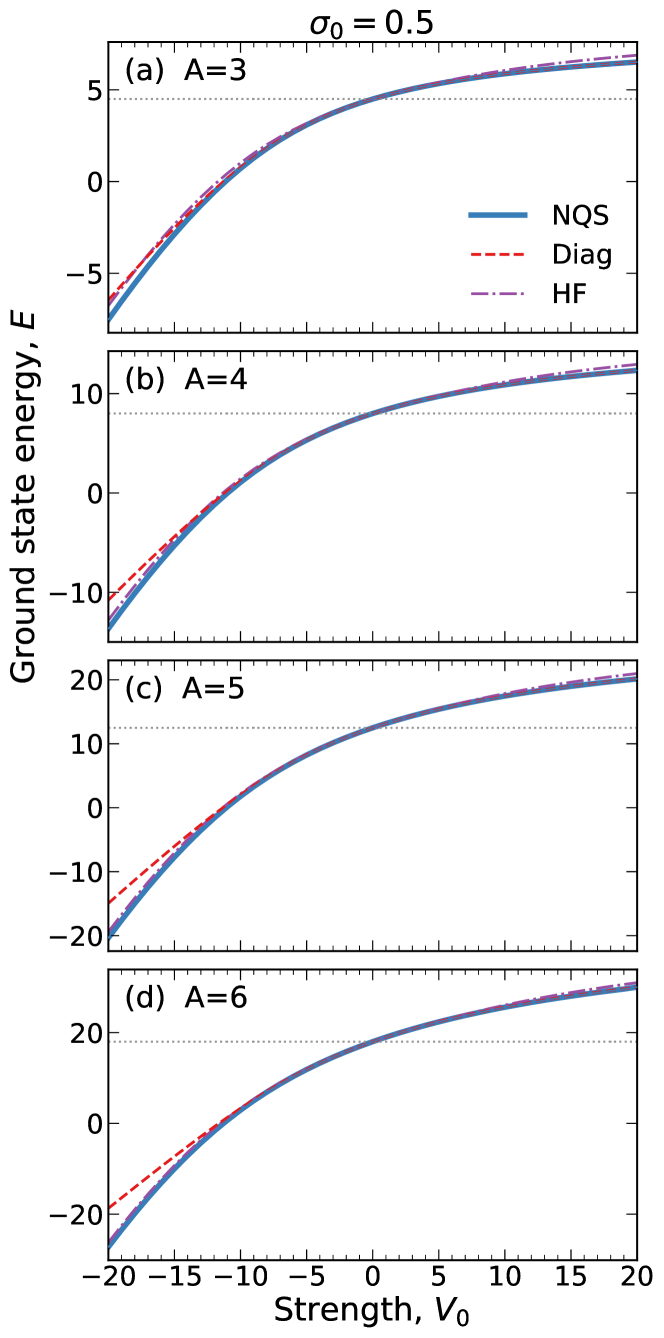
Figure 9: The ground-state energy of the $A$-particle system as a function of interaction strength, $V_{0}$, for a fixed range, $\sigma_{0}=0.5$. Panels (a) to (d) correspond to systems of $A=3$ to $A=6$ particles. See Fig. 6 for an explanation of the legend.

IV.2.1 Energy

We start by considering the energy of the system. Figures 9(a)-9(d) show the energy for $A=3$ to $6$ particles as a function of $V_{0}$. We focus on the case with a range value of $\sigma_{0}=0.5$. The qualitative behavior of the energy in all these systems is very similar to that in the $A=2$ case. On the repulsive side, the system energy increases slowly and tends to plateau at a value which is about $1.25-1.6$ times the noninteracting value. In this repulsive range, a power-law scaling with the particle number $E\approx A^{2.2}$ approximates the complete results well. The saturation of the energy as $V_{0}$ becomes very repulsive bodes well with the physical picture of a crystal. This picture is further reinforced by the density profiles, which we present later. In the attractive regime, in contrast, the energy per particle decreases much more steeply as a function of $V_{0}$, with no signs of saturation as $V_{0}$ becomes more negative.

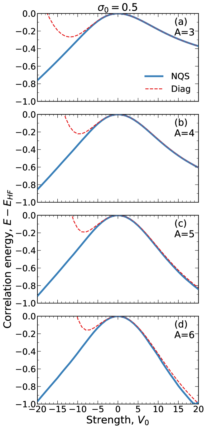
Figure 10: The correlation energy of the $A$-particle system as a function of interaction strength, $V_{0}$, for a fixed range, $\sigma_{0}=0.5$. Panels (a) to (d) correspond to systems of $A=3$ to $A=6$ particles. See Fig. 6 for an explanation of the legend.

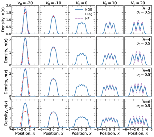
Figure 11: Density profiles $n(x)$ as a function of position $x$ for different values of $V_{0}$ and a fixed range $\sigma_{0}=0.5$. From left to right, $V_{0}$ goes from $-20$ to $20$ in increments of $10$ units. From top to bottom, we show the results for $A=3$, $4$, $5$ and $6$ particles.

In terms of benchmarks, we notice two different remarkable tendencies. First, the HF results overestimate the ground-state energy, as expected due to the lack of backflow. The difference between the HF and the NQS prediction becomes less noticeable as the particle number increases. In other words, the HF approximation becomes more reliable in relative energy terms as the number of particles increases. This is not so surprising, since the mean-field picture should work better as the number of particles increases. Second, we find that the exact diagonalization technique is always less bound than the NQS prediction for values $V_{0}<-10$. We interpret this as a consequence of the finite model space, which is insufficient in this strongly attractive regime. Anticipating the results of Fig. 11, in the bosonized regime the density of the system is substantially more compressed than in the noninteracting HO case. One may thus expect to need many more single-particle modes to describe the density profile and the energetics of the system.

To quantify further the importance of correlations in the system, we look at the correlation energy for the $A=3$ to $6$ particles as a function of $V_{0}$ in Fig. 10. We stress that the energy scale is the same for all panels. In other words, the difference between the HF and the full result appears to be relatively constant independently of the particle number. On the repulsive regime at $V_{0}=20$, the energy increases by about $0.2$ units every time that we add one more particle to the system. In contrast, the increase on the attractive size is less steep. We stress that in the NQS the nonzero correlation energy is a direct consequence of the backflow correlations in the Ansatz. It is remarkable that this extension allows the NQS to capture the asymmetric dependence on correlation energy with $V_{0}$, due to the different phases of the system.

In the attractive side, the direct diagonalization approach yields a relatively poor description of the correlation energy. Nonphysical, positive values of $E_{c}$ are achieved for coupling constants below $V_{0}<-10$ or $-15$. On the repulsive size, we also find signs of a relatively poorer description of the correlation energy with the direct diagonalization approach for $A\approx 6$. Having said that, it is clear that the direct diagonalization approach works much better in the repulsive side, where deviations from the NQS prediction are within $0.05$ in absolute energy terms.

IV.2.2 Density profiles

It is also very useful to inspect the density profiles, $n(x)$, of the systems with $A=3$ to $6$ particles. We summarize these results in Fig. 11, where the columns correspond to different interaction strengths and the rows correspond to different numbers of particles. We compare predictions from the NQS (solid), the direct diagonalisation approach (dashed) and the HF approximation (short-dash-dotted lines).

The middle panels, corresponding to the noninteracting case ($V_{0}=0$), show $A$ peaks on top of a Gaussian-like overall behavior. This is an expected behavior, which arises as a result of Eqs. (3) and (27). In the attractive regime, the peak-like fermionic structure in the density profile disappears from $V_{0}\approx-10$ onwards. The NQS results show a single peak that becomes narrower as $V_{0}$ becomes more attractive. This is in line with the HF prediction, which approaches the NQS result as the number of particles increases. In contrast, the direct diagonalization approach is unable to grasp the narrow density distribution beyond $V_{0}\leq-10$. At $V_{0}=-20$, the NQS and HF density distributions are almost a factor of $2$ narrower than the noninteracting case. It is thus naïvely expected that a model space truncation in the direct diagonalization cannot capture such strong density rearrangements.

In the strongly repulsive limit, $V_{0}\gg 0$, the interaction effectively separates the fermions apart, leading to the full crystallization of the system [85, 88]. The separation of single-particle orbitals, however, cannot proceed indefinitely because the harmonic trap is more and more effective as $|x|$ increases. While the position of the $A$ density peaks barely changes, the troughs between them become more and more defined as $V_{0}$ increases. In this repulsive regime, the direct diagonalization for the density profile results coincide with the NQS predictions. In contrast, the HF approach fails substantially. The HF density profiles overestimate (underestimate) the peaks (troughs) and the disagreement becomes more pronounced as the number of particles increases. We stress that the differences in density profiles arise from the existence of backflow correlations in our NQS Ansatz. More details on the density profile and the average size of the system are provided in Ref. [30].

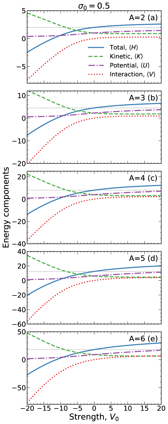
Figure 12: Different components of the NQS ground-state energy as a function of interaction strength, $V_{0}$, for a fixed range $\sigma_{0}=0.5$. Solid, dashed, dash-dotted and dotted lines correspond to the total, kinetic, harmonic oscillator and interaction energies, respectively. Panels (a) to (e) correspond to systems of $A=2$ to $A=6$ particles. The horizontal dotted line is the noninteracting ground-state energy.

The difference of the density profiles in the attractive and repulsive regimes is reflected into the energetics of the system. We show different contributions to the total energy as a function of the interaction strength $V_{0}$ in Fig. 12. Panels from top to bottom correspond to different numbers of particles, from $A=2$ (top) to $A=6$ (bottom). We distinguish the contributions due to the kinetic energy, $\langle K\rangle=\langle\Psi|\sum_{i}-\frac{\partial_{i}^{2}}{2m}|\Psi\rangle/\langle\Psi|\Psi\rangle$; the (external) harmonic oscillator potential energy, $\langle U\rangle=\langle\Psi|\sum_{i}-\frac{x_{i}^{2}}{2}|\Psi\rangle/\langle\Psi|\Psi\rangle$; and the interaction energy, $\langle V\rangle=V_{0}/(\sqrt{2\pi}\sigma_{0})\langle\Psi|\sum_{i<j}e^{-(x_{i}^{2}-x_{j}^{2})/2\sigma_{0}^{2}}|\Psi\rangle/\langle\Psi|\Psi\rangle$. These components are all computed stochastically using the NQS wave function probability.

We find a common picture, which is relatively independent of the particle number. In the noninteracting case, the virial theorem stipulates that $\langle E\rangle=2\langle K\rangle=2\langle U\rangle$ (and $\langle V\rangle=0$). In the repulsive side, the harmonic oscillator and the interaction energy components increase very slowly as $V_{0}$ grows. We interpret this slow growth in terms of localization. When the single-particle orbitals become localized into $A$ well-defined, equidistant peaks, the sharpening of the fermionic features only modifies these two components slightly. In contrast, the kinetic energy reduces substantially as a function of $V_{0}$. In fact, for particle numbers $A>4$, we observe that $\langle K\rangle\leq\langle V\rangle$, a condition that is typically employed to characterize a (Wigner) crystal [88].

The analysis in terms of different energy components indicates that the energy in the attractive regime behaves rather differently. First of all, we find that the attractive total energy in the regime where $V_{0}\ll 0$ is the result of the cancellation of two large but opposite energy components. On the one hand, the kinetic energy $\langle K\rangle$ increases substantially as $V_{0}$ decreases, as a result of the strong density rearrangement. On the other, the interaction energy $\langle V\rangle$ becomes extremely attractive as all the particles are confined near the center of the trap and, consequently, near each other. The central confinement also leads to a near cancellation of the harmonic-oscillator potential energy $\langle U\rangle$.

At this stage, we can draw some conclusions about the nature of the correlations in the repulsive and attractive sides of the spectrum. Clearly, the bosonic transition in the attractive side leads to a very strong rearrangement of the density profile. This rearrangement is so strong, in fact, that the direct diagonalization based on noninteracting single-particle states struggles to capture it. An accurate description of this transition requires instead the solution of the system in real (or, possibly, momentum) space. We note that qualitatively similar results for the density profiles of $A=3$ and $4$ spinless fermions are reported by Schilling et al. [56] employing an even parity harmonium model. A universal bosonic peak for attractive interactions was observed in that case too.

In contrast, the rearrangement of the density in the repulsive regime mostly leads to a localization of single-particle states that exaggerates the associated fermionic features. This is also found in the few-body system with an harmonium model [56]. The HF approach in this limit, however, overestimates the fermionic features, which again highlights the importance of backflow correlations.

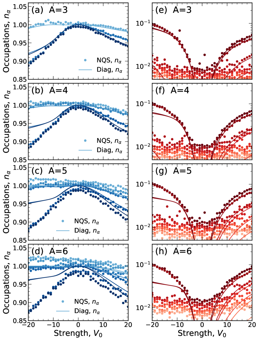
Figure 13: Panels (a)-(d): hole ($\alpha<A$) occupation probabilities for the $A=3$ (top row) to the $A=6$ (bottom row) systems as a function of interaction strength $V_{0}$ for a fixed range $\sigma_{0}=0.5$. We compare NQS results (solid circles) to the direct diagonalisation predictions (solid lines). Panels (e)-(h): the same, in logarithmic scale, for particle ($\alpha\geq A$) states up to $\alpha=14$.

IV.2.3 Occupation numbers

We get further insight on the correlation structure of the system by looking at the occupation numbers, $n_{\alpha}$, for different single-particle states $\alpha$. We show $n_{\alpha}$ for systems with $A=3$ (top row) to $A=6$ (bottom row) in Fig. 13. The left (right) hand panels correspond to the occupation probabilities of holes (particles), $n_{\alpha<A}$ ($n_{\alpha\geq A}$). There are distinct common structures appearing in the occupation numbers in the attractive and the repulsive regimes. In the attractive case, the NQS predicts the appearance of one doubly degenerate state that becomes substantially depleted as $V_{0}$ becomes more and more negative. This result is commensurate with the direct diagonalization occupation prediction, which also appears to be double degenerate, although, somewhat less depleted. We interpret the difference between the NQS and the direct diagonalization prediction, again, as a sign of the truncated model space. Both the NQS and the diagonalization predictions indicate that the remaining $A-2$ hole states are fully occupied to within a $2\%$ accuracy, although, the statistical noise floor in the NQS approach makes it difficult to quantify this statement.

The particle states shown in Figs. 13(e)-13(h) show the appearance of a doubly-degenerate state in the repulsive regime for all values of $A$. According to the NQS prediction, these states reach an occupation of $\approx 10\%$ at $V_{0}=-20$. These doubly-degenerate states are reminiscent of a bosonization of the fermionic degrees of freedom. This happens in spite of the absence of active spins and hence can only be observed in the case of a finite-range interaction. Doubly degenerate structures in the attractive regime have also been observed in variational calculation of one-dimensional (1D) $p$-wave fermions [42]. These simulations, however, have a harder time describing the repulsive regime, which the NQS can access seamlessly.

In the repulsive regime, $V_{0}>0$, no double degeneracy is observed. Single-hole states [Figs. 13(a)-13(d)] and single-particle states [Figs. 13(e)-13(h)] are all distinct, and one can clearly distinguish $A$ states on the repulsive branch of each panel with occupations $n_{\alpha}>5\times 10^{-3}$. This prediction is supported both by the direct diagonalization and the NQS results. For the $A=3$ system, Fig. 13(a), we find that three distinct single-hole states appear with small depletions, with occupations of more than $95\%$ up to $V_{0}\approx 20$. The corresponding single-particles states in Fig. 13(e) are clustered into two nearly degenerate states with populations of $\approx 5\%$ at $V_{0}\approx 20$, and another state with a population of $2\%$. A similar picture emerges as $A$ increases. For even values of $A$, we find that there is a near (but not complete) degeneracy of $A/2$ states. In the single-hole cases, the occupations decrease steadily with $V_{0}$ in pairs. Similarly, the occupation of particle states increases in pairs of similar values. For odd $A$, the picture is essentially the same, except that there is an odd single-particle orbital with a specific occupation probability. We note that there are similarities between this picture and the results obtained in Ref. [56] for 1D spin-polarized trapped fermions with harmonic pair interactions.

For both the single-particle and single-hole states, the statistical noise floor is on the order of $\approx 10^{-2}$. We find a slight increase of this floor with particle number, of about a factor of $2$ when moving from $A=3$ to $A=6$. Although one can see the statistical noise within the single-particle states, their effect is even more evident in the single-hole states, where they lead to nonphysical fluctuations with $n_{\alpha}>1$. We arbitrarily limit the number of single-particle states to $14$ within this analysis. The noise floor is consistent for all values of $V_{0}$, indicating that its source stems from the stochastic methodology used to calculate the OBDM. We limit the range of occupation values shown for the single-hole states to be above $5\times 10^{-3}$, which highlights a few of the lowest single-hole states obtained with the direct diagonalization approach (solid lines).

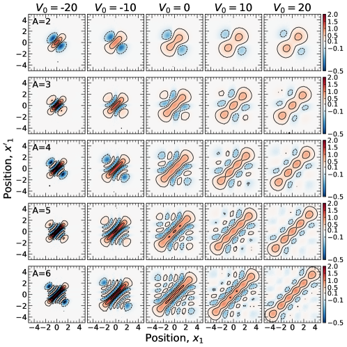
Figure 14: Density contour plots of the one-body density matrix $\rho(x_{1}^{\prime},x_{1})$ of systems from $A=2$ (top row) to $A=6$ (bottom row) particles. Columns correspond to different interaction strengths, from $V_{0}=-20$ (left column), to $V_{0}=20$ (right). Contours are shown at density matrix values of $-0.5$, $-0.1$, $0.1$, $0.5$, $1.0$, $1.5$ and $2.0$. The colour coding is the same across all panels.

IV.2.4 One-body density matrix

So far, we have discussed local properties of the system. We now turn our attention to nonlocal structures reflected in the density matrices. We discuss the NQS results in this and the following sections, and refer the reader to the Appendix for the analogous HF and direct diagonalization results. In Fig. 14, we show the OBDM $\rho(x_{1}^{\prime},x_{1})$ of the ground-state wave function for $A=2$ (top row) to $A=6$ (bottom row). The different columns correspond to interaction strengths values from $V_{0}=-20$ to $20$ (in steps of $10$). The central panels correspond to the noninteracting case, $V_{0}$, which can be understood in relatively simple analytical terms from a combination of Eq. (27), valid in the noninteracting case, and the HO eigenstates of Eq. (3), leading to Eq. (10) [57]. In all cases, the density matrix is purely real, and covers a more-or-less square area in the $x_{1}^{\prime}-x_{1}$ plane. This is a consequence of the combination of single-particle terms $\varphi_{n}^{*}(x_{1}^{\prime})\varphi_{n}(x_{1})$ in the sum of Eq. (27), which naturally provide a limit both within and outside the diagonal of the $x_{1}^{\prime}-x_{1}$ plane [94]. This is clearly seen in Eq. (10), which indicates that $\rho(x_{1}^{\prime},x_{1})$ is given by a Gaussian envelope in the $x_{1}^{\prime}-x_{1}$ modulated by a polynomial.

Moreover, one finds that there is a relatively narrow area of positive values near the diagonal, where $\rho(x^{\prime}=x,x)\equiv n(x)>0,$ is positive definite. As one moves away from the diagonal, definite ripples appear in areas with consecutive positive and negative values. These ripples reflect the nodal structure of the single-particle states. In fact, there are as many changes of sign along the $x_{1}^{\prime}=-x_{1}$ direction in one side of the diagonal as particles in the system. Equation (10) provides an explanation of this in terms of the roots of the polynomials of order $2(A-1)$ along the $x_{1}^{\prime}=-x_{1}$ direction.

In the attractive case, shown in the left panels, the overall size extent of the system decreases (see Fig. 11). Similarly, the support of the OBDM in the $x_{1}^{\prime}-x_{1}$ plane also diminishes. Moreover, the peaks and troughs associated to the changes of sign in the off-diagonal direction move closer to the diagonal. Importantly, these interference effects appear to increase in magnitude as the interaction strength becomes more negative. We stress that the diagonalization of this strongly oscillating OBDM leads to occupation numbers with a dominant doubly degenerate structure, more reminiscent of a coherent picture.

In the strongly repulsive case, in the panels on the right, one can clearly distinguish the localization of single-particle orbitals along the diagonal in the form of well-defined equidistant peaks. The off-diagonal oscillations and change of signs observed in the non-interactive and the attractive regimes, are substantially damped in this case. At $V_{0}=20$, for instance, one only observes a well-defined series of $A-1$ quasicircular regions with negative values in a direction parallel to the diagonal. While there are additional oscillations along the off-diagonal direction, these have a much smaller amplitude, to the point that they can hardly be distinguished in the scale of the figure.

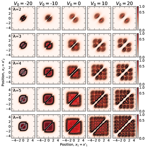
Figure 15: Density contour plots of the pair correlation function $g(x_{1},x_{2})$ for systems from $A=2$ (top row) to $A=6$ (bottom row) particles. Columns correspond to different interaction strengths, from $V_{0}=-20$ (left column), to $V_{0}=20$ (right). Contours are shown at steps of $0.05$ from $0$ to $0.35$ (solid lines), and at steps of $0.2$ from $0.4$ to $2$ (dashed lines). The colour coding is the same across all panels.

IV.2.5 Pair correlation function

Finally, we present in Fig. 15, the PCF, $g(x_{1},x_{2})$ of Eq. (11) for different particle numbers. The panels are organized in the same way as Fig. 14. The PCF provides information of correlations due both to the antisymmetric nature of the system and to the presence of interactions [54]. The function $g(x_{1},x_{2})$ is very different in the attractive and the repulsive regimes, but there are common structures across all panels. Specifically, we find a ridge around $x_{1}\approx x_{2}$ where the pair correlations vanishes. This is a consequence of the Pauli exclusion principle, which in the spinless fermion case imposes the condition $g(x,x)=0$. In the noninteracting system, the condition is enforced by the $(x_{1}-x_{2})^{2}$ term of Eq. (12). The width of this “Pauli ridge”, however, changes substantially with interaction strength, which indicates that part of it is also a consequence of interaction effects. On the repulsive side, shown on the panels to the right of the center, one clearly finds that the ridge becomes wider with $V_{0}$. This effect is a reflection of the spatial localization of the orbitals observed in Figs. 7 and 11. We expect the size of the ridge in the repulsive side to be sensitive to both $V_{0}$ and the range of the interaction, $\sigma_{0}$. As $V_{0}$ is more repulsive, particles try to localize more, leading to more distant and well-defined peaks in the PCF.

In contrast, on the attractive regime displayed on the left panels of the figure, we find that the ridge becomes narrower as $V_{0}$ becomes more attractive, to the point that, for $A>5$, the ridge is difficult to see on the leftmost panels with $V_{0}=-20$. The pair distribution function in the attractive side is relatively featureless and, other than the ridge, it is extremely peaked in an almost square region around the center. This indicates a high likelihood of finding one particle in a region within a few units of position of the center, a picture that is reminiscent of a Bose-Einstein condensate. This picture is in line with the PCF of two spinless fermions with a soft-core potential [41] and of the correlation structure of P-wave fermions observed in Ref. [42].

In contrast with this relatively featureless peak, $g(x_{1},x_{2})$ on the repulsive side has a much richer structure, with several well-defined peaks. These peaks are clear indications of the emerging localized structure of the system, and have been observed in analogous simulations of one-dimensional, few-body Wigner crystals [85]. For odd particle numbers, we find that there is always a peak to the right (or left) of the Pauli ridge along the $x_{1}=0$ direction. For these systems, the density has a peak at $x=0$ (see Fig. 11), so one particle sitting at $x_{1}=0$ will have a large probability of finding $A-1$ particles at fixed intervals in $x_{2}$. For $A=3$, this occurs at $x_{2}=\pm 2$, whereas for $A=5$ this happens at about $x_{2}=\pm 1.5$ and $\pm 3$.

The structure for an even number of particles is relatively different. For an even number of particles, there is a depletion in the density distribution at the center of the trap, see Figs. 7 and 11. Consequently, the PCF along $x_{i}=0$ does not show any peaks. Instead, the lines of horizontal or vertical $A-1$ peaks are found at around $x_{i}\approx\pm 1$. Whereas for $A=4$ particles a second set of three peaks is found at $x_{i}=\pm 2.5$, for $A=6$ particles this is localized at $x_{i}=\pm 2$. The well-defined single-particle peaks are therefore more compressed as $A$ increases, in line with the results of Fig. 11.

All in all, the PCF for all systems indicates a well-defined localized phase in the repulsive regime, and a Bose-like phase in the attractive regime. This complex behavior is obtained with an NQS formed by a single determinant with backflow correlations. In other words, for a fixed particle number, the same NQS is capable of describing systems with very different spatial extents, correlation structures and underlying physical pictures. We take this as a promising sign for the performance of NQS approaches in the description of condensed matter systems.

V Conclusion and outlook

To conclude, we have applied the NQS method to solve the Schrödinger equation for one-dimensional systems of $A$ harmonically trapped, interacting fermions without spin degrees of freedom. We model the interaction using a toy model Gaussian form factor, motivated by nuclear physics applications and such that, in the zero-range limit, we recover the noninteracting case. We purposely choose a set of interaction strengths and ranges where perturbation theory may not converge easily. In particular, we find that an interesting choice for the interaction range is half the natural oscillator length.

The NQS that we employ provides a fully antisymmetric Ansatz to represent one-dimensional “spinless” fermions. The NQS has two equivariant layers of $H=64$ hidden nodes each. These layers embed the one-dimensional positions of $A$ particles into a $H$-dimensional space. These layers are then projected into a single GSD. This approach benefits from backflow correlations from the outset, and does not explicitly require a Jastrow factor. The number of parameters of the NQS remains nearly constant when going from $A=2$ to $A=6$ particles. By combining the NQS with VMC techniques, we obtain a wave function that is able to represent many-body correlations and can accurately describe very different physical regimes without any specific modifications to the network architecture.

The focus of our paper is on benchmarking the new NQS approach with other well-known many-body methods. For all values of $A$, we compare against the mean-field Hartree-Fock method and the direct diagonalization approach. Moreover, in the $A=2$ case we have access to an exact solution in real space as well as a perturbative treatment of the Gaussian interaction. The results for all values of $A$ indicate that the NQS can efficiently provide an accurate representation of the many-body wave function. One benefit of the NQS approach formulated in the real-space continuum is its variational performance, that surpasses mean-field approaches and does not suffer from basis truncation effects, like the direct diagonalization method does. We characterize our benchmarking process using several properties, including the ground-state energy, density profiles, single-particle occupation numbers, as well as the one-body density matrix and the PCF.

The NQS can accurately describe the ground-state wave function across different physical regimes. In particular, we find two very different pictures that arise as the strength of the interaction goes from very attractive to very repulsive values. We find a common, method-independent interpretation for these two phases of 1D trapped spinless fermionic systems. On the attractive side, the density distribution of the system is a single peak centered at the origin, reminiscent of a Bose-Einstein condensate. The peak becomes narrower and higher as the strength becomes more negative. This represents a substantial density rearrangement in the system, that is hard to capture with a truncated basis direct diagonalization approach based on an harmonic-oscillator basis. A real-space implementation of the Hartree-Fock method, however, describes well this phase for sufficiently large $A$. In this regime, the one-body density matrix is strongly oscillating off the diagonal and the pair distribution function is narrow and squared shaped. We find that a degenerate set of $2$ single-particle orbitals are strongly depleted, whereas the remaining $A-2$ states remain fully occupied.

Figure 16: The same as Fig. 14 for the Hartree-Fock approximation.

In contrast, for large and repulsive values of the interaction strength we find a completely different picture. In this limit, we reach the regime of a localized crystal, and fermions spontaneously order in a periodic fashion. This is reflected in the density distribution, which has a well-defined periodic structure, with $A$ peaks, as well as the PCF, which shows associated crystalline structures. In terms of occupation numbers, the repulsive regime exhibits quasidegeneracies in pairs of orbitals. We note that this regime is well described by the direct diagonalization approach, but the HF approximation predicts density distributions with exaggerated localization features.

We foresee several applications of this work in the near future, and distinguish between applied and formal developments. On the applied side, we have found clear signatures of two physical phases in relatively simple fermionic systems. When spin is not present, finite-range interaction effects are necessary and lead to very different behavior in the attractive and repulsive regime. Here, one may exploit NQSs to investigate physical features that have not been explored yet, like higher-order density matrices. Moreover, one could also employ the NQS wave function to compute matrix elements of other relevant operators employing standard Monte Carlo techniques [61]. Having access to the full wave function of the system, we should also be able to characterize the evolution of entanglement measures as a function of interaction parameters. It would be interesting to perform NQS simulations with odd-parity potentials, which resemble the more realistic interactions employed in the past in spinless fermion studies [39, 37, 35]. We stress that there is no fundamental limitation hampering the applicability of the NQS method for derivative odd-parity potentials. In addition, one could extend this approach to other trapped systems, with hard boundary conditions [95], or to infinite systems incorporating periodic boundary conditions [20, 96, 97].

On the formal side, there are interesting step forwards to take in a variety of directions. First, it would be interesting to quantify the quality of the wave function Ansatz in more formal terms. In other words, one could try and gauge what information is lost when introducing this NQS Ansatz. A potential avenue may involve the quantification of entanglement measures on NQS. In applications of one-dimensional ultracold atoms, spin degrees of freedom are relevant, and often manipulated experimentally. This calls for an explicit, general spin-dependent representation of NQSs, along the lines recently explored in lattice systems [98], nucleons [33], the electron gas [20, 96] or unitary fermions [97], but potentially applicable to SU($N$) interactions. A comparison with the rich variety of experiments in nonperturbative regimes here may provide a fertile ground for tests of the applicability of NQS Ansätze. Finally, our findings indicate that an NQS originally pretrained in a noninteracting case can eventually learn at least two different phases of a quantum system. It would be interesting to analyze whether this result is general, and whether NQSs can indeed perform across complex quantum phase-transition boundaries.

Our ultimate aim is the study of nuclear physics systems employing NQSs. To this end, we need to extend our current technology to treat three-dimensional systems. This also requires the inclusion of spin and isospin degrees of freedom. All studies so far indicate that nuclei in the few-body sector can be theoretically accessed by employing NQSs [29, 31, 32, 33]. It remains to be seen whether the promising scaling with particle number that we have found in this work can be efficiently transferred into a nuclear physics setting and deliver a substantial change in ab initio nuclear theory.

Figure 17: The same as Fig. 15 for the Hartree-Fock approximation.

Appendix A Non-local properties

In this Appendix, we look at the nonlocal properties obtained with our benchmarks models. We provide, specifically, an analysis of the OBDM and PCF obtained within the HF approximation and within the direct diagonalization framework. On the one hand, this provides a useful cross-check with the NQS results of the main text. On the other, it allows us to identify the effect of correlations in the nonlocal properties of the system.

A.1 Hartree-Fock

We start by discussing the results of Fig. 16, which shows the OBDM in the HF approximation. The format and panel structure is the same as shown for the NQS data in Fig. 14: different rows correspond to particle numbers from $A=2$ to $A=6$ and different columns indicate different interaction strengths for $\sigma_{0}=0.5$. Qualitatively, Figs. 14 and 16 are very similar. In the attractive regime (panels to the left of the center), we find that the system becomes more compact as $V_{0}$ becomes more negative. Just as in the NQS case, the HF solution shows a strong oscillatory behavior off the diagonal. In contrast to the NQS solution, however, the central ridge in the HF results is higher and the overall support of the density matrix has a more well-defined, square shape.

The central column shows the same results for the NQS and the HF solution, as expected since this is a noninteracting case. Nonetheless, this is a nontrivial check on the numerical accuracy of the NQS solution, which thus reproduces not only the energy but also the nonlocal properties of the noninteracting wave function. On the repulsive side, shown in the panels to the right of the center, the HF results are also very similar to the NQS data shown in Fig. 14. In the HF solution, we find that there is more structure concentrated along the diagonal, with more localized solutions and clearly identifiable peaks compared to the NQS simulations. This bodes well with the findings of the density profiles shown in Fig. 11. Off the diagonal, the NQS results show a slightly stronger oscillatory behavior than the HF predictions.

We now discuss the PCF within the HF approximation, which we show in Fig. 17. Here, the format is the same as Fig. 15 in the main body of the text. Just as in the case of the OBDM, the central column of the two cases is the same. This indicates, again, that the noninteracting case is under control with the NQS Ansatz. This benchmark indicates that the NQS Ansatz does not lose any significant amount of information at the two-body level.

Differences between the HF and NQS pair distribution functions can be observed in both the attractive and repulsive regimes. In the attractive case, the support for the HF correlation functions is smaller than in the NQS case. This is in line with the corresponding density distributions, which are narrower in the HF case. In addition, the HF case shows a sharper, square-like behavior in the attractive cases and a somewhat narrower Pauli ridge.

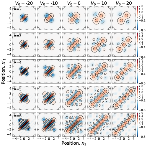
Figure 18: The same as Fig. 14 for the direct diagonalization approach.

In the repulsive case, the HF densities show a much more localized state. In the pair distribution function, this translates into very well-defined peaks. The peaks in the HF distribution lie close to those predicted by the NQS, but are generally rounder and higher.

A.2 Direct diagonalization

We have also computed the OBDM and the PCF for the direct diagonalization simulations. We already know from the analysis of the energetics, the local densities and the occupation numbers that the exact diagonalization solution has convergence issues in the attractive regime. We therefore expect to see differences in this sector, which should be taken as indications of the lack of numerical convergence associated with the truncation of the finite model space as opposed to any actual physical limitations.

We show in Fig. 18 the OBDM obtained from the exact diagonalization approaches in the same format as Figs. 14 and  16. As expected, there are virtually no observable differences in the central and right panels of the Figures. In this regime, the exact diagonalization results are well converged and the agreement with the NQS can be taken as a solid qualitative benchmark. In other words, the one-body nonlocal properties of the NQS wave function are well under control.

On the attractive regime, in the panels left of the center, we observe increasing differences as the interaction strength $V_{0}$ and the particle number $A$ increase. The lowest-left panel, with $V_{0}=-20$ and $A=6$, is the most affected in this case. We find a density matrix with extended support in the $x_{1}-x_{1}^{\prime}$ plane. Off the diagonal, we observe the same number of oscillations in the NQS and the exact diagonalization cases, but the latter shows a larger, less compact oscillation structure. We assume that this is due to the absence of high energy modes in the active space, which may be able to account for faster off-diagonal oscillations.

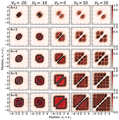
Figure 19: The same as Fig. 15 for the direct diagonalization approach.

Finally, Fig. 19 shows the PCF extracted from the exact diagonalization approach. On the noninteracting and the repulsive columns, there are no notable differences between the NQS results of Fig. 15 and the direct diagonalization results. Again, this can be taken as an indication of the high-quality NQS wave function. Just as in the case of the OBDM, the differences between the NQS and the exact diagonalization method increase with $A$ and are more visible for the more attractive values of $V_{0}$. In accordance with the observations of the local density profiles of Fig. 11 and the OBDM of Fig. 14, the direct diagonalization results tend to have a more compact PCF, which also features some very faint oscillations off the diagonal. We attribute these again to the truncation of the many-body basis in the exact diagonalization approach.