Multiple steady states and symmetry breaking in a stably stratified, valley-shaped enclosure heated from below

Abstract

We delineate the complete structure of steady laminar flows within a stably stratified, valley-shaped triangular cavity heated from below through linear stability analysis and Navier-Stokes simulations. Our formulation follows Prandtl’s idealization of mountain and valley flows. We derive an exact solution to the quiescent conduction state, which bifurcates to two pairs of flow patterns with symmetric and asymmetric circulations in the valley-shaped cavity. We characterize the flow via the stratification perturbation parameter, $\Pi_{s}$, which is a measure of the strength of the surface heat flux relative to the strength of the background stable stratification, while keeping other dimensionless parameters fixed. At very low $\Pi_{s}$ values, the pure conduction state remains stable. Beyond a threshold value of $\Pi_{s}$, a unique bifurcation event transpires, giving rise to two discernible types of eigenmodes. One type is marked by a single dominant circulation positioned at the valley’s center, while the other one exhibits dual circulations of equal strength within the same central valley region. Notably, the critical value associated with the central-circulation eigenmode is marginally lower than that of the dual-circulation eigenmode. Through three-dimensional Navier-Stokes simulations, we confirm that the central-circulation eigenmode generates a pair of asymmetric steady states, whereas the dual-circulation eigenmode leads to distinct upslope and downslope symmetric convection patterns. The dissimilarity between the two dual-circulation patterns originates from the absence of a horizontal symmetry axis ($x$-axis) within the geometry. Linear stability analysis and three-dimensional Navier-Stokes simulations jointly confirm the linear instability of the two dual-circulation states, indicating that the slightest asymmetric perturbation will induce a transition towards the asymmetric steady state. Overall, our investigation reveals that, for a given set of dimensionless parameters, the Navier-Stokes equations admit at least five possible steady-state solutions. Two of these solutions, namely the quiescent, pure conduction state as well as the counter-intuitive symmetric downslope state, have previously been overlooked in stably stratified valley-shaped cavities heated from below. Additionally, we show that, contrary to previous studies, the asymmetric flow state is the primary and expected state due to the instability of the symmetric state at all parameter values investigated here.

I Introduction

During an atmospheric evening transition in regions of complex terrain, surface cooling induces downslope, or katabatic winds. These katabatic winds contribute to the development of a stably stratified cold pool in valleys, which persists throughout the night. During the morning transition, surface heating prompts upslope, or anabatic flows, opposing the stably stratified cold pool’s presence and eventually causing its dissolution. Notably, numerical weather prediction models often encounter challenges when dealing with stably stratified flows in complex terrain [1], as well as the transitions between nocturnal stably stratified periods and daytime intervals [2]. These limitations can adversely impact the accuracy of predictions regarding morning fog formation and pollutant dispersion [3, 4]. Consequently, our objective is to enhance the comprehension of stably stratified flows experiencing surface heating within an idealized valley setting.

In this study, we adopt Prandtl’s idealization for mountain and valley flows that assumes a constant ambient or background stratification independent of the thermal forcing at the surface [5, 6]. To this end, the presence of an ambient stable stratification sets our problem apart from Rayleigh-Bénard type convective flows because of the expanded set of dimensionless numbers governing the flow problem. Our choice of a V-shaped enclosure represents an idealized geometry for valley flows, facilitating the examination of fundamental instabilities and flow patterns. Additionally, this selection establishes connections with prior experimental research [7, 8] and lays the groundwork for forthcoming experiments concerning flow regimes and instabilities.

Thermal convection in attic-shaped (an inverted valley geometry) triangular cavities with isothermal conditions on sloped walls without any stratification effects have been studied [9]. In such configurations, a symmetric convection pattern prevails at low Grashof numbers, and a subcritical pitchfork bifurcation occurs at larger parameter values leading to a steady asymmetric circulation state [10, 11], which has been shown to agree with smoke flow visualizations in an attic-shaped triangular cavity with a finite depth [12].

In comparison to attic-shaped cavities, there has been relatively less attention on convection in V-shaped enclosures with ambient stratification. Princevac and Fernando [7] conducted experiments with stratified saline water in a V-shaped tank heated with a constant heat flux on bottom walls to represent morning transition in valleys in a laboratory setting. They introduced the dimensionless breakup parameter $B$, along with the slope angle of the valley walls, to characterize flow patterns that form along the sloping walls. Motivated by the experiments of Princevac and Fernando, Bhowmick et al. [13] used two-dimensional (2D) Navier-Stokes (N-S) simulations to investigate flow dynamics in triangular V-shaped cavities heated from below with an initially stratified fluid and adiabatic conditions on the top boundary. Their 2D simulations produced symmetric circulation patterns within the valley-shaped cavity. Bhowmick et al. [14, 15] also performed 2D N-S simulations for valley-shaped cavities heated from below and cooled from the top boundary without any stratification effects. A common dynamics that was observed in these 2D N-S simulations as a function of increasing Rayleigh number is the establishment of a steady symmetric circulation transitioning to a steady-state asymmetric circulation through a pitchfork bifurcation, which is proceeded by the emergence of a periodic state through a Hopf bifurcation.

Our present investigation establishes additional connections with aforementioned studies that involve convection in triangular cavities and other widely recognized convection phenomena. Particularly pertinent to our study is the presence of multiple feasible steady-state solutions in a convection problem with an ambient stable stratification. Multiple steady-state solutions in convection problems were demonstrated by Gelfgat et al. [16] in the context of Rayleigh-Bénard convection, and likewise for other confined, convective flows [17]. Venturi et al. [18] illustrate that in Rayleigh-Bénard convection, the single-roll convection pattern is often favored over the two-roll state due to its heightened heat transport efficiency. This tendency is similarly observable in geophysical models of ocean dynamics. Marotzke et al. [19] employ an idealized meridional-plane model to investigate ocean thermohaline circulation, uncovering the existence of multiple equilibrium states, including an unstable symmetric state that transitions into an asymmetric state upon minor perturbation. Correspondingly, Bryan [20] scrutinizes the same configuration through a three-dimensional general circulation model of the ocean, yielding analogous findings.

Several dimensionless parameters have found use in prior studies for characterizing stratified flows with surface heating, as well as stratified flows in cavities. In a series of papers, Xiao and Senocak [21, 22] established the stratification perturbation parameter $\Pi_{s}$ in the context of Prandtl’s idealization of mountain and valley flows. This parameter signifies the ratio between the imposed surface heat flux and the stabilizing background stratification, and it serves as a basis for assessing the dynamical stability of the Prandtl model concerning katabatic and anabatic slope flows. In the context of stratified flows within cavities, J. Yalim, J. M. Lopez, and B. D. Welfert [23] employed the buoyancy number —a measure of the ratio between viscous and buoyancy timescales —to examine the instability of a stably-stratified fluid within a square cavity undergoing vertical oscillations. Similarly, Grayer et al. [24] utilized this parameter to explore the dynamics of stably stratified flow in a tilted square cavity with differentially heated side walls. Furthermore, the experimental work conducted by Princevac and Fernando [7] in a stratified water tank heated from below introduced the so-called break-up parameter $B$ to track the disintegration of stratification within an initially stably stratified V-shaped valley. In the next section, we show that the break-up parameter is expressible as a combination of the stratification perturbation parameter, the buoyancy number, and the Prandtl number.

The current study examines instabilities and steady-state convection patterns within a stably stratified valley-shaped enclosure heated from below. We investigate a set of conditions that have not been previously explored using linear stability analysis and three-dimensional (3D) simulations of the Navier-Stokes equations. Specifically, we extend the dimensionless parameter space for the studied configuration, scrutinizing transitions between various potential flow states within a multi-stable arrangement. We apply a constant positive heat flux to both bottom walls of the valley-shaped enclosure, which parallels the experimental setup outlined in Princevac and Fernando [7]. Simultaneously, we enforce a fixed temperature at the upper boundary, thereby establishing conditions conducive to a pure conduction state. Utilizing the stationary, pure conduction steady state as our starting point in these investigations holds a distinct advantage. In such cases, linear stability and nonlinear energy stability are in agreement [25]. This alignment allows us to comprehensively capture the exact bifurcation of the flow at the first critical stability threshold through linear stability analysis—an outcome corroborated by our validation through 3D Navier-Stokes simulations. Additionally, our approach encompasses a constant background stable stratification, unaffected by the thermal forcing at the surface. This approach aligns with Prandtl’s idealization of mountain and valley flows [5, 21], and thus the current study represents an extension of Prandtl’s model to anabatic flows in idealized valleys. Although similarities can be drawn between our current arrangement and the dynamics observed in comparable scenarios, such as Rayleigh-Bénard convection, the distinctive factor in our present study is the introduction of an extra dimensionless parameter due the presence of a constant stable stratification of the ambient environment, which adds a forcing term to the buoyancy equation, which is absent in typical Rayleigh-Bénard configurations. Notably, Xiao and Senocak [26] demonstrated that this ambient stratification plays a crucial role in modeling stably stratified flows, even over flat surfaces.

II Technical formulation

A schematic of the computational domain is shown in Figure 1, where $H$ is the height of the domain and $\alpha$ is the slope angle of the walls of the valley-shaped enclosure relative to the $x$ axis. The enclosure lies in the $x-y$ plane, with the homogeneous $z$ direction into the page. Thus $u$ represents the horizontal velocity in the $x$ direction, $v$ represents the vertical velocity in the $y$ direction, and $w$ represents the spanwise velocity in $z$ direction. We perform linear stability analysis (LSA) in only the two-dimensional (2D) valley geometry, and thus we only present 2D instabilities resulting from our LSA. However, our Navier-Stokes simulations are conducted with all three dimensions resolved to ensure that the observed instabilities are two dimensional.

The buoyancy is related to the potential temperature $\Theta$ by $b=g\left(\Theta-\Theta_{e}\right)/\Theta_{r}$, where $\Theta_{e}$ is the potential temperature of the ambient environment, and $\Theta_{r}$ is a reference potential temperature. A constant background stratification is imposed through the buoyancy frequency, or Brunt-Väisälä frequency, given by $N=\sqrt{\left(g/\Theta_{r}\right)\partial\Theta_{e}/\partial y}$ in the buoyancy transport equation (see the last term in equation 3). Thus $b$ represents a scaled perturbation of the full potential temperature $\Theta$ from the linear background stratification defined by $\Theta_{e}$, manifested in the constant $N$.

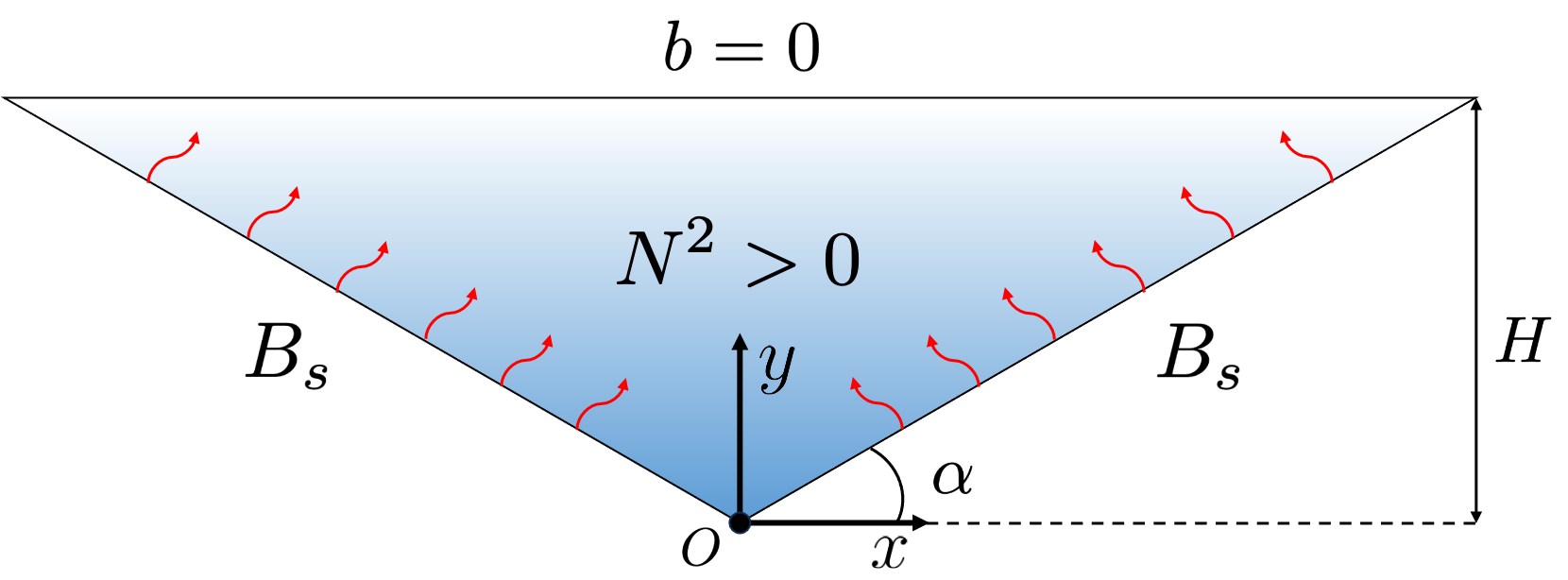
Figure 1: Schematic of the computational domain with key external parameters.

The continuity, momentum, and buoyancy equations, with the Boussinesq approximation, can be written as follows:

$$\nabla\cdot\mathbf{u}=0,$$ (1)

$$\frac{\partial\mathbf{u}}{\partial t}+\mathbf{u}\cdot\nabla\mathbf{u}=-\nabla p+\nu\nabla^{2}\mathbf{u}+b\mathbf{g},$$ (2)

$$\frac{\partial b}{\partial t}+\mathbf{u}\cdot\nabla b=\beta\nabla^{2}b-N^{2}\mathbf{g}\cdot\mathbf{u},$$ (3)

where $p$ is the specific pressure including a constant reference density $\rho_{0}$, $\nu$ is the kinematic viscosity, $\beta$ is the thermal diffusivity, and $\mathbf{g}$ represents the effective gravity vector, $\mathbf{g}=[0,1,0]$, acting only in the $y$ direction. Here, the last term of equation (3) should be noted, as this additional term in the buoyancy equation arises due to the constant background stratification defined by $N$. This term arises from the formulation by Prandtl [5] and separates the current analysis from simple Rayleigh-Bénard convection in a triangular cavity, as pointed out by Prandtl.

The boundary conditions for buoyancy include a constant, positive buoyancy flux on the two bottom walls, defined as $B_{s}=\beta\partial b/\partial n$, where $n$ is the direction normal to the sloping bottom boundaries, and where a positive $\partial b/\partial n$ refers to heating of the fluid. On the top boundary, a constant $b=0$ is imposed. For velocity, a no-slip condition is imposed on the two bottom walls, and a free-slip condition is imposed on the top boundary. These boundary conditions are chosen to parallel the experimental study of Princevac and Fernando [7] which consists of water in a V-shaped tank with a free surface on top. However, unlike the experiments which consist of high Reynolds number flows, we focus on the dynamics near the stability threshold, meaning we only investigate laminar flows in the absence of an ambient wind.

Under these conditions, the following exact solution with zero velocity for $p$ and $b$ to Equations 2 and 3 can be derived

$$p(y)=\frac{-B_{s}}{2\beta\cos\alpha}\left(y-H\right)^{2},\qquad b(y)=\frac{B_{s}}{\beta\cos\alpha}\left(H-y\right).$$ (4)

This motionless steady state within the heated valley is only possible due to the constant buoyancy imposed at the top boundary combined with the constant heat flux at the sloped surfaces, which admits a linear buoyancy and quadratic pressure profile as a solution. Equation (4) represents the motionless, pure conduction state in the enclosure and will be used as a base flow for our linear stability analysis. For 3D nonlinear simulations, all variables are periodic in the homogeneous $z$ direction with a length of twice the height of the valley-shaped enclosure.

We use the following scales to normalize dimensional quantities:

$$l_{0}=H,\quad u_{0}=\sqrt{\frac{B_{s}}{N}},\quad b_{0}=\frac{B_{s}H}{\beta\cos\alpha},\quad p_{0}=\frac{B_{s}H^{2}}{\beta\cos\alpha},\quad t_{0}=H\sqrt{\frac{N}{B_{s}}},$$ (5)

where the length scale, $l_{0}$, is defined as the height of the valley geometry, and the timescale is the convection timescale, $t_{0}=l_{0}/u_{0}$. An alternative length scale could be defined as half of the valley width, $l_{0}=H/\tan\alpha$, and the stratification timescale can be defined as $t_{0}=1/N$. The height was chosen as the length scale to more conveniently non-dimensionalize the base flow, and the convective timescale is used throughout the rest of the present study as it better describes the timescale of the evolution of the present instabilities. The vorticity is defined as the curl of the velocity, $\mathbf{\omega}=\nabla\times\mathbf{u}$, but due to the purely 2D nature of the instabilities investigated here, we refer only to the vorticity in the $z$ direction, $\omega_{z}$, with a corresponding scale $\omega_{0}=u_{0}/l_{0}$.

Using the physical scales defined in equation (5), we non-dimensionalize the governing equations (1-3) and obtain the following:

$$\nabla\cdot\mathbf{u}=0,$$ (6)

$$\frac{\partial\mathbf{u}}{\partial t}+\mathbf{u}\cdot\nabla\mathbf{u}=-\frac{\Pi_{h}}{\cos\alpha}\nabla p+\frac{Pr}{\sqrt{\Pi_{s}\Pi_{h}}}\nabla^{2}\mathbf{u}+\frac{\Pi_{h}}{\cos\alpha}b\mathbf{g},$$ (7)

$$\frac{\partial b}{\partial t}+\mathbf{u}\cdot\nabla b=\frac{1}{\sqrt{\Pi_{s}\Pi_{h}}}\nabla^{2}b-\frac{\cos\alpha}{\Pi_{s}}\mathbf{g}\cdot\mathbf{u}.$$ (8)

Similarly, the analytical solution for the pure conduction state simplifies to

$$p(y)=-\frac{1}{2}\left(y-1\right)^{2},\qquad b(y)=1-y,$$ (9)

where all variables are now in their non-dimensional form. From equations (6-8), we see that flow in a valley-shaped enclosure under stable stratification is controlled by four dimensionless parameters, defined as,

$$\Pi_{s}=\frac{B_{s}}{\beta N^{2}},\quad\Pi_{h}=\frac{NH^{2}}{\beta},\quad Pr=\frac{\nu}{\beta},\quad\alpha,$$ (10)

where $Pr$ is the Prandtl number, and $\alpha$ is the slope angle. The dimensionless stratification perturbation parameter, $\Pi_{s}$, first introduced to characterize the stability of Prandtl slope flow [21] is key to the present investigation. $\Pi_{s}$ is a measure of the strength of the imposed surface buoyancy gradient relative to the stabilizing background stratification. In Prandtl slope flows, the higher the $\Pi_{s}$ the more dynamically unstable and turbulent the flow becomes [22]. The dimensionless parameter, $\Pi_{h}$, is a new addition and related to the buoyancy number $R_{N}$ [23, 24] by $\Pi_{h}=PrR_{N}$, and represents the ratio between the thermal diffusion and buoyancy time scales.

We note that the set of dimensionless parameters given in equation (10) is larger than the set adopted in previous studies of stratified flows in valley-shaped enclosures. For example, Princevac and Fernando [7] introduce the dimensionless breakup parameter $B=N^{3}H^{2}/B_{s}$, along with $Pr$ and $\alpha$, whereas the Rayleigh number was used in Bhowmick et al. [13]. In light of the expanded parameter space given in equation (10), we observe that $B$ is a combination of two independent dimensionless parameters $B=\Pi_{h}/\Pi_{s}$. In this way, we can say that four dimensionless parameters are needed to fully describe the flow dynamics.

II.1 Linear stability analysis

We linearize equations (1-3) around an arbitrary base flow defined by $(U_{i},\bar{p},\bar{b})$, and assume disturbances take the form of waves given by

$$\mathbf{\hat{q}}(x,y,t)=\left[\hat{u}(x,y),\hat{v}(x,y),\hat{w}(x,y),\hat{p}(x,y),\hat{b}(x,y)\right]\exp\left(\omega t\right),$$ (11)

where $\mathbf{\hat{q}}$ represents the vector of 2D disturbance quantities, and $\omega$ represents the temporal growth rate. Substitution of the above disturbance quantities into the linearized Navier-Stokes equations leads to the following generalized eigenvalue problem

$$\mathbf{A}\mathbf{\hat{q}}(x,y)=\omega\mathbf{B}\mathbf{\hat{q}}(x,y).$$ (12)

By solving the eigenvalue problem, we can determine the global linear stability behavior of the given base flow for a 2D valley-shaped enclosure. The real part of the growth rate, $\mathrm{Re}(\omega)$, indicates whether an infinitesimal disturbance will exponentially grow, when $\mathrm{Re}(\omega)>0$, or decay, when $\mathrm{Re}(\omega)<0$, while the imaginary part, $\mathrm{Im}(\omega)$, indicates the temporal frequency of the resulting mode of instability. All simulations were carried out using the spectral/hp element code Nektar++ [27, 28], which has been widely validated for a variety of flow problems. All simulations are run with a finite element discretization of 31 elements along the bottom walls with a polynomial order of 4 within each element. The eigenvalue problem is solved using the modified Arnoldi method available in Nektar++, and it is found that refinement in our spectral element mesh results in very little to no change in the eigenvalue (0.1% difference near the critical value), which provides confidence in our results.

Numerical integration of the full 3D Navier-Stokes equations was performed with Nektar++ to produce steady-state profiles, as well as to obtain and validate secondary states arising from the primary instabilities. For 3D simulations, we resolve the dimensionless spanwise extent of the valley ($L_{z}=2$) with 32 Fourier modes. Navier-Stokes simulations are performed with both initially 2D disturbances, defined by the eigenmodes obtained from LSA, as well as 3D random disturbances. The inclusion of the third direction in the Navier-Stokes simulations is to ensure the 2D dynamics observed are not based on a lack of consideration of the third direction.

III Results

III.1 Primary linear stability analysis

We first perform two-dimensional (2D) linear stability analysis (LSA) of the valley-shaped enclosure with a zero velocity base flow with the pressure and buoyancy profiles given in equation (4). In all the simulations and analyses, slope angle $\alpha$ and $\Pi_{h}$ are fixed at $30^{\circ}$ and $1500$, respectively. Prandtl number $Pr$ is set to $7.0$ to parallel the experimental study of Princevac and Fernando [7]. We only vary $\Pi_{s}$ throughout the study.

For small values of $\Pi_{s}$, meaning the perturbation caused by the surface buoyancy flux is small compared to the stabilizing background stratification, the quiescent, pure conduction state is stable. As we increase $\Pi_{s}$, this base state becomes linearly unstable, and LSA reveals two eigenmodes at critical $\Pi_{s}$ values, shown in Figure 2. The imaginary part of the eigenvalue of both modes is zero, indicating they are non-oscillatory.

The vorticity field and streamlines for the first eigenmode, displayed in Figure 2a, shows that it consists of one large circulation in the center alongside smaller, counter-rotating corner vortices. The buoyancy profile, shown in Figure 2b, depicts how the central circulation advects heat away from the hot bottom walls and how the colder fluid near the top wall recirculates down towards the surface. For these reasons, we refer to this eigenmode as the central-circulation eigenmode. An examination of the velocity and buoyancy field of this eigenmode reveals that it satisfies the symmetry of reflection about the $y$ axis for the linearized N-S equations. Specifically, this can be defined by the transformation $\mathcal{C}_{1}$:

$$\mathcal{C}_{1}:\left[u,v,b,p\right]\left(x,y\right)\mapsto\left[u,-v,-b,-p\right]\left(-x,y\right).$$ (13)

The central-circulation eigenmode is invariant under this transformation, and thus we refer to it as symmetric with respect to this transformation, or $\mathcal{C}_{1}$-symmetric in short. However, it should be noted that while the linearized N-S equations are invariant under this transformation, this is not true of the full N-S equations due to the nonlinear convective terms, and this fact will have implications on the nonlinear evolution of the eigenmode.

Figure 2: Visualization of eigenmodes resulting from linear stability analysis of analytical base flow for $\Pi_{s}=0.9$, showing (a) vorticity and (b) buoyancy of the central-circulation eigenmode, and (c) vorticity and (d) buoyancy of the dual-circulation eigenmode. Line integral convolution (SurfaceLIC) is used to visualize vector fields, and buoyancy profiles are shown with isotherms.

The second eigenmode, shown in Figures 2c and 2d, consists of two identical, counter-rotating main circulations on each side of the valley center. The buoyancy profile, Figure 2d, shows that the direction of the two central circulations is downslope, which can be seen through the high temperature in the center of the valley. This suggests that the eigenmode exists in both upslope and downslope configurations. While the emergence of two possible states from a given eigenmode is not surprising, we note here that the downslope configuration represents flow traveling down the heated bottom walls, which is a counter-intuitive state that would not be able to be discovered without performing modal stability analysis on the quiescent, pure conduction base state. Because this eigenmode is characterized by two circulations of equal strength in the center of the valley, we refer to this eigenmode as the dual-circulation eigenmode. Similar to the central-circulation, this eigenmode also satisfies a symmetry of reflection about the $y$ axis, although differs from the one previously defined. The symmetry can be defined by the transformation:

$$\mathcal{C}_{2}:\left[u,v,b,p\right]\left(x,y\right)\mapsto\left[-u,v,b,p\right]\left(-x,y\right).$$ (14)

The dual-circulation eigenmode is invariant under the transformation $\mathcal{C}_{2}$, and thus we say it is symmetric with respect to $\mathcal{C}_{2}$, or $\mathcal{C}_{2}$-symmetric in short. Unlike the $\mathcal{C}_{1}$ transformation, it can be shown that both the linearized and full N-S equations and boundary conditions are invariant under the $\mathcal{C}_{2}$ transformation. In other words, for any flow state in the valley $\mathbf{u}$, the transformed flow $\mathcal{C}_{2}(\mathbf{u})$ is also a solution. We also note that the action of this transformation creates a mirror image of the original flow state reflected about the vertical axis. Thus the symmetry of the dual-circulation eigenmode is only possible due to the symmetry of our valley geometry.

Beside the strongest circulation cells, each eigenmode also exhibits a series of progressively smaller eddies towards each corner. Moffatt [29] studied the case of a sequence of eddies in a sharp corner due to a purely hydrodynamic (i.e. no thermal effects) motion in the fluid far from the corner with the Stokes equation, and predicted that an infinite sequence of eddies occurs in the corner with quickly diminishing strength. From an inspection of the eigenmodes, we can distinguish five distinct eddies in the central-circulation state, which can be observed due to the line integral convolution in Figure 2a, and six eddies in the dual-circulation state, the smallest two being too weak to be visualized in the corners in Figure 2c. Additional eddies can likely be identified with increased resolution in the corners, but we assume that any additional eddies are small enough in strength and size to have no effect on the overall flow. The progression of eddies we observe do not decrease in strength as strongly as predicted by Moffatt, and the ratio of the maximum $u$ velocity along the top boundary varies between the main circulation to the secondary circulations, and the secondary circulations to the corner eddies. The drop-off in strength between the main circulation and the secondary circulations is approximately 5 for the central-circulation case and approximately 12 for the dual-circulation case, whereas the drop-off between the secondary circulations and the corner eddies is approximately 100 for the central-circulation case and 600 for the dual-circulation case. The differences from the theory of Moffatt can be explained by the heated sloping walls in our case, which provides buoyancy force up the wall towards the corner along the entire wall, while Moffatt’s results are derived from a purely hydrodynamic motion of the fluid far from the corner.

The reason for the onset of the central and dual-circulation instabilities can be explained from consideration of the dimensionless $\Pi_{s}$ parameter. For very small $\Pi_{s}$ values, the zero flow state can remain stable due to the conduction of the heat through the fluid, as well as the stabilizing effect of the background stratification, but as the surface heating increases, the stabilizing effect of the stratification is overcome, and convection begins to dissipate the additional heat.

The growth rate of each of the eigenmodes is plotted against $\Pi_{s}$ in Figure 3. Each exhibits a roughly linear trend in growth rate in the unstable regime. A line is fit to these unstable points to give an estimate of the critical $\Pi_{s}$ value for each eigenmode. We find that the critical value of the dual-circulation eigenmode to be approximately $0.875$, whereas for the central-circulation eigenmode it is approximately $0.872$. The slope of the linear trend of growth rate against $\Pi_{s}$ is found to be 1.91 for the dual circulation, and 1.95 for the central circulation. Thus, the central circulation has a lower critical value than the dual circulation, and the growth rate of the central circulation grows faster with $\Pi_{s}$ in comparison to the dual circulation. Both of these findings indicate that the central-circulation eigenmode is the most unstable mode in a perfectly symmetric external configuration.

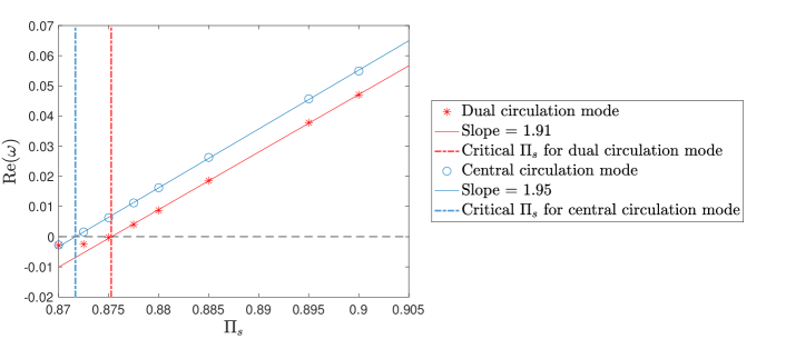
Figure 3: Growth rate of dual-circulation and central-circulation instabilities versus $\Pi_{s}$. Critical values are estimated based on the linear trend of the positive growth rates.

III.2 Steady-state Navier-Stokes solutions

Next, we perform time-integration of the 3D Navier-Stokes equations, equations (1-3), to obtain the steady-state solutions arising from the central and dual-circulation instabilities. Initial conditions for each simulation were defined by the analytical base flow, equation (4), plus a small multiple of the eigenvector for each of the unstable eigenmodes. In this way, we can observe the initial exponential growth of the disturbance, and compare it to the growth rate predicted by LSA. It should be noted that while we perform 3D simulations with $L_{z}=2$, all eigenmodes are two dimensional, which lead to only 2D steady states. Additionally, we run a simulation of $\Pi_{s}=0.9$ with $L_{z}=16$ with an initial random 3D disturbance, which ultimately settles to a steady 2D state that is identical to our results with a 2D initial disturbance field. Thus we can be confident that our assumption of 2D disturbances is not spurious due to lack of consideration of the third direction. The 2D circulation patterns in our 3D simulations agree qualitatively with the experimental smoke visualizations of Holtzman et al. [12] who investigated convection in attic-shaped cavities with finite depth.

From the eigenvectors shown in Figure 2, we observe that the central-circulation eigenmode shows a clockwise main circulation, and the dual-circulation eigenmode shows two main circulations that travel down the sloping valley walls. These two eigenmodes represent four possible steady-state velocity profiles: the central-circulation state being either clockwise or counterclockwise, and the dual-circulation state being either upslope or downslope. Through manipulations of the initial eigenvector disturbance to our simulations, we can obtain steady-state profiles for each of these four states, as shown in Figure 4.

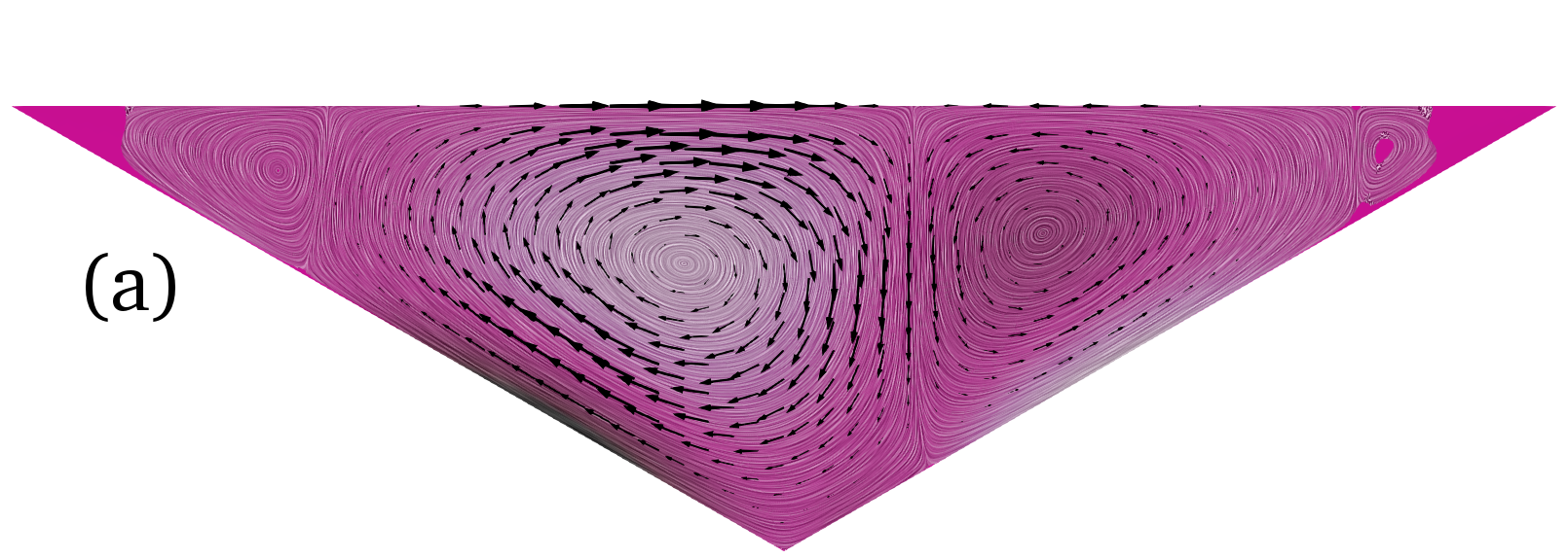
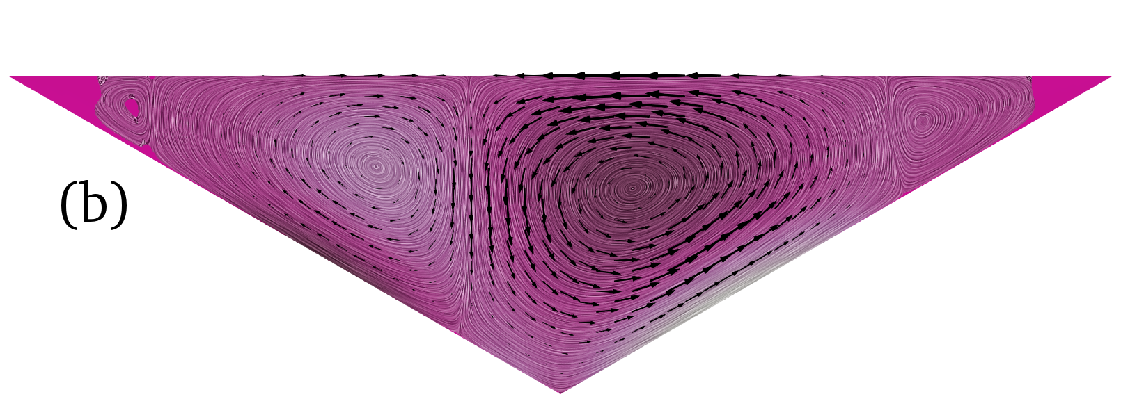
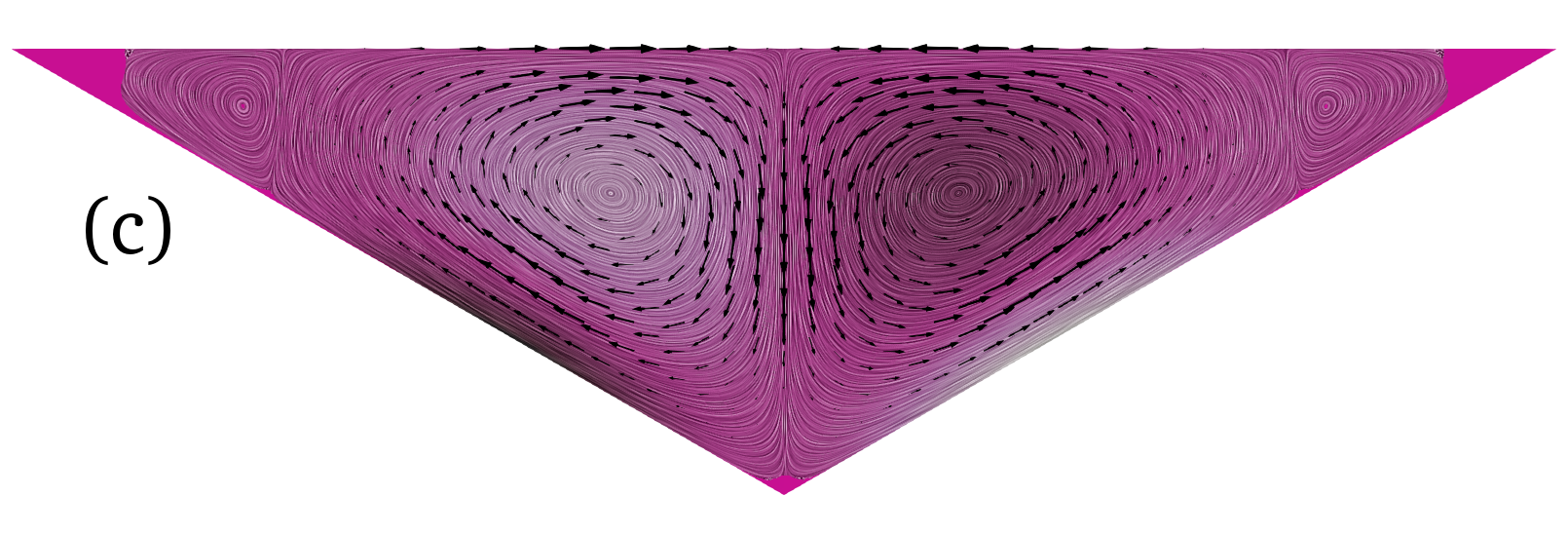
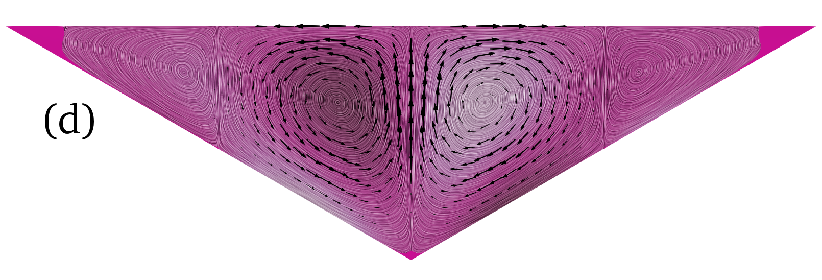
Figure 4: Visualization of vorticity along with velocity vectors of four possible steady-state solutions resulting from the central-circulation and dual-circulation eigenmodes at $\Pi_{s}=0.9$: (a) Central circulation, clockwise, (b) central circulation, counterclockwise, (c) dual circulation, upslope, (d) dual circulation, downslope.

Focusing first on the central-circulation states shown in Figures 4a and 4b, we can see that each is an exact reflection of the other about the $y$ axis, which can be explained by the symmetry of the valley geometry and the symmetry of the N-S equations about the $y$ axis. The steady-state profiles of the central-circulation state vary significantly from the corresponding eigenvector, shown in Figure 2a, and these steady-state profiles are no longer symmetric about the $y$ axis. This is due to the fact, as stated earlier, that the transformation which defines the symmetry of the central-circulation eigenmode $\mathcal{C}_{1}$ is not invariant under the full N-S equations, and thus the $\mathcal{C}_{1}$-symmetry of the eigenmode cannot be maintained in the nonlinear evolution.

The process by which the $\mathcal{C}_{1}$-symmetric central-circulation eigenmode evolves to the asymmetric steady state is shown in Figure 5, which shows the vorticity and velocity vectors at different times in the evolution. An animation depicting this evolution can be viewed in the Supplementary Material [30]. In the period from $t_{n}=0$ to $t_{n}=2$, the initial eigenmode disturbance exponentially increases in strength and maintains the symmetry, shown in Figure 5a. As the velocity continues increasing, the nonlinear convective terms come into play, and by $t_{n}=4$, the symmetry of the initial disturbance is broken, seen in Figure 5b. As time progresses, the strong, now asymmetric, central circulation diminishes in intensity, as can be seen in comparison of Figure 5c and d to 5b. The location of the dominant central circulation slowly migrates from the slight left center of the valley (Figure 5c at $t_{n}=6$) to the slight right of the valley center in the final state (Figure 5f at $t_{n}=20$). This is accompanied by a change in strength of the secondary circulations in the corners of the valley. At early time in the evolution, for $t_{n}$ from approximately 4 to 8, the circulation in the right corner of the valley is clearly the stronger of the two corner circulations, most clearly seen in Figure 5b and c. However, as the primary circulation moves to occupy more of the right side of the valley, this secondary circulation is diminished (Figure 5d and e), and the secondary circulation in the left corner grows in strength until it clearly has a larger strength as the flow converges to the steady state (Figure 5f). This process occurs in order to have both the primary circulation and the smaller secondary circulation exhibit primarily upslope flow along the heated bottom walls. While flow profiles with downslope configurations are possible, they are inherently unstable in the given configuration, and thus flows profiles with upslope flow dominating the side walls are preferred.

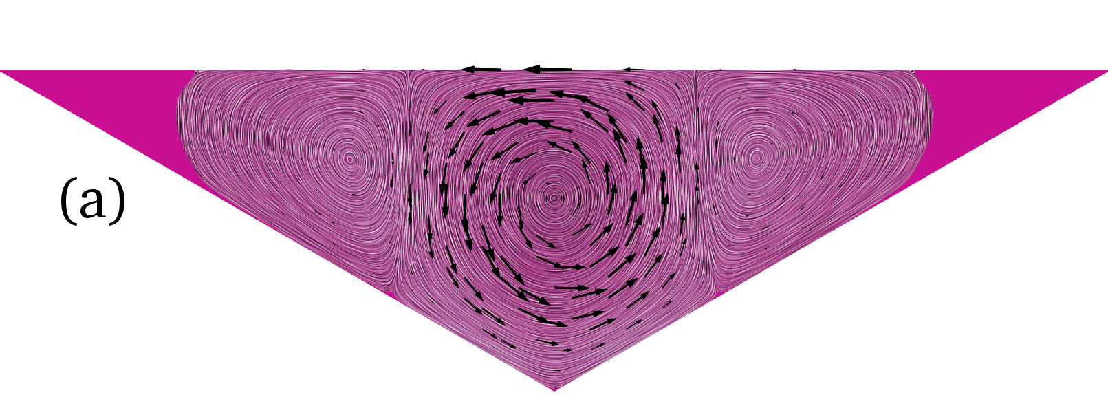
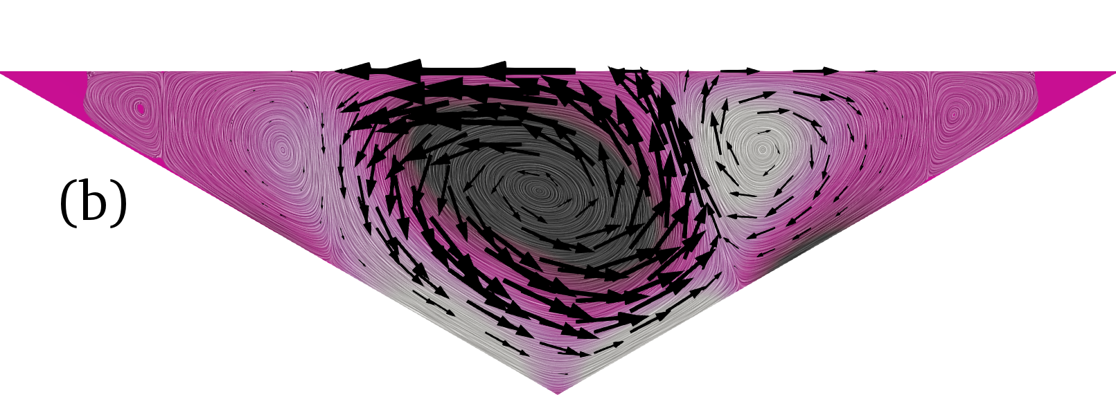
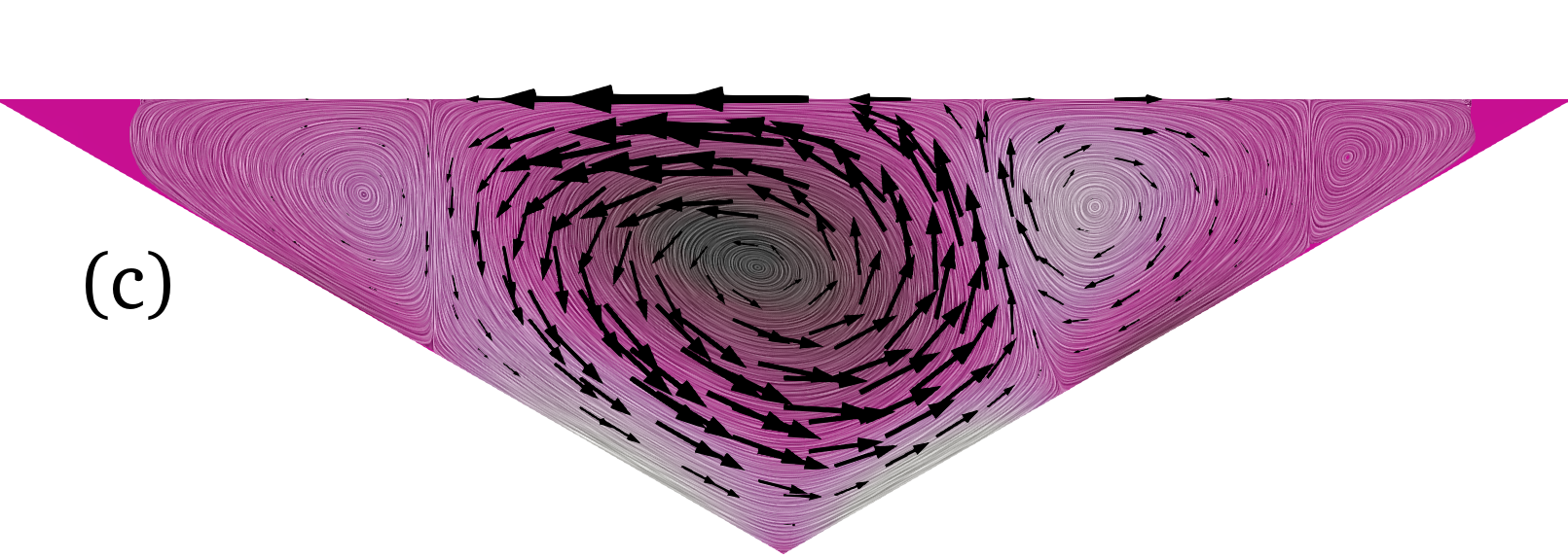
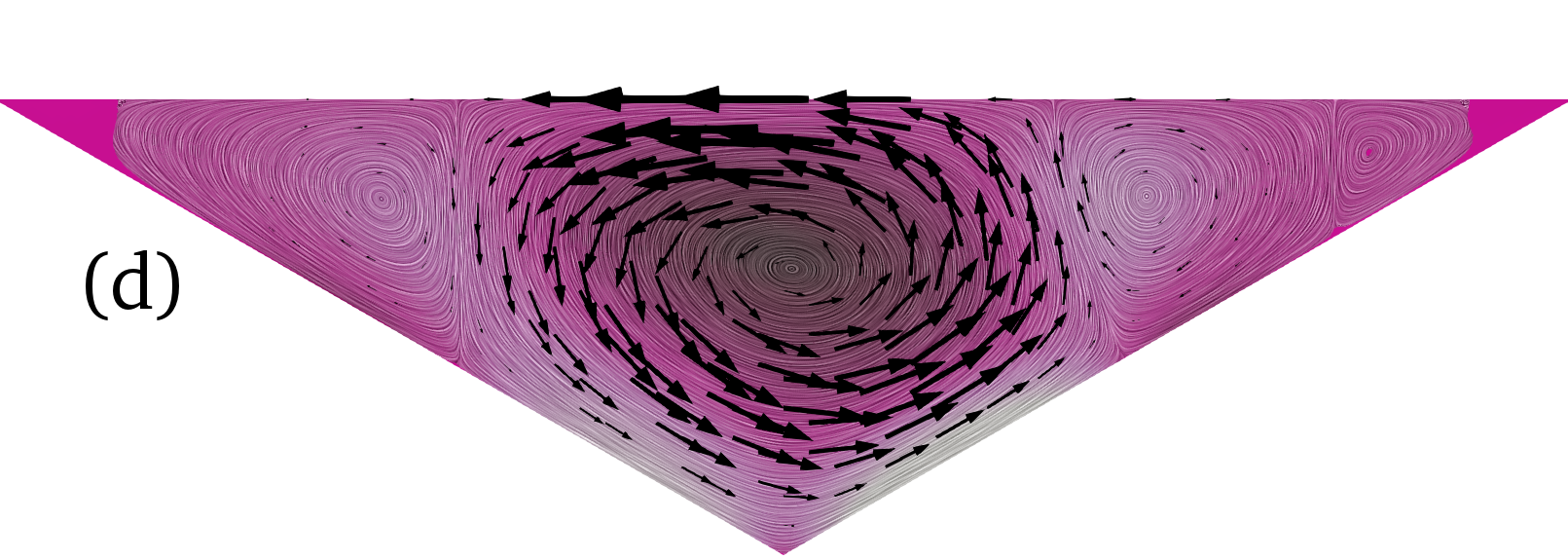
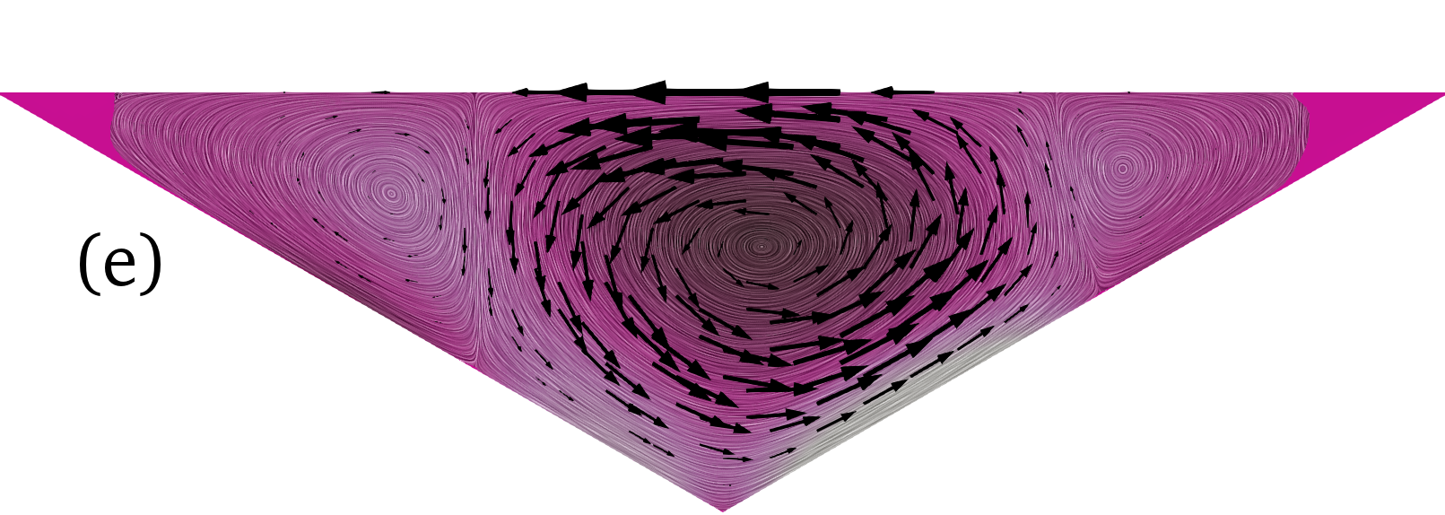
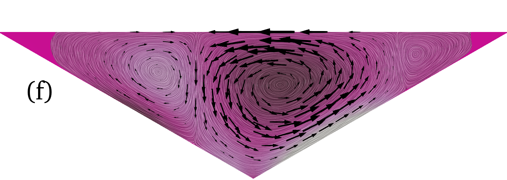
Figure 5: Visualization of vorticity over time for the nonlinear simulation starting with the central-circulation eigenmode and evolving to the asymmetric, counterclockwise steady-state profile. Dimensionless times shown are (a) $t_{n}=2.10$, (b) $t_{n}=3.94$, (c) $t_{n}=6.04$, (d) $t_{n}=8.92$, (e) $t_{n}=12.08$, and (f) $t_{n}=19.94$. The video of this evolution can be viewed in the Supplementary Material [30].

The nonlinear evolution leaves a new asymmetric steady-state profile, asymmetric in that each individual state, Figures 4a and b, satisfies no symmetry about the $y$ axis with itself. Thus, the central-circulation eigenmode, although the eigenmode itself is $\mathcal{C}_{1}$-symmetric, leads to symmetry breaking in the valley when considering the full N-S equations. In fact, we see that while each steady-state solution is asymmetric, meaning no transformation leads to the same identical state, applying the $\mathcal{C}_{2}$ transformation to the state with the clockwise central circulation yields the exact other steady state with the counterclockwise circulation, and vice versa.

In order to visualize how this symmetry breaking occurs over time as the central-circulation eigenmode evolves to the asymmetric steady state, we define a symmetric projection that projects any state into a new state that is $\mathcal{C}_{1}$-symmetric. This symmetric projection state can be defined as $\mathbf{u}_{\mathrm{sym}}=0.5(\mathbf{u}-\mathcal{C}_{2}(\mathbf{u}))$, where $\mathbf{u}$ is the original state, and $\mathcal{C}_{2}(\mathbf{u})$ is the $\mathcal{C}_{2}$ transformation of the original state. As previously stated, $\mathcal{C}_{2}(\mathbf{u})$ represents the mirror image reflection of $\mathbf{u}$ about the $y$-axis, and thus the subtraction of the two creates a $\mathcal{C}_{1}$-symmetric profile, $\mathbf{u}_{\mathrm{sym}}$. If the two fields are added instead of subtracted, the resulting symmetric projection is rather $\mathcal{C}_{2}$-symmetric. The difference between the original state $\mathbf{u}$ and its symmetric projection $\mathbf{u}_{\mathrm{sym}}$ is then calculated, and the kinetic energy (KE) of this difference is integrated over the area of the valley. In Figure 6, we calculate the KE difference for each time over the evolution of the central-circulation eigenmode to its ultimately asymmetric steady state. This difference can be interpreted as a degree to which the $\mathcal{C}_{1}$-symmetry is broken. For example, if the original state is invariant under $\mathcal{C}_{1}$, it is identical to its symmetric projection and the KE difference is exactly zero. This can be seen at early times ($t_{n}<2$) as the symmetry is preserved and the KE difference remains zero. After this, we see a spike at approximately $t_{n}=4$, corresponding to the state pictured in Figure 5b, before the state becomes more symmetric as the central circulation moves back towards the center (for $t_{n}$ approximately 5 to 10, corresponding to Figure 5c and d). Beyond $t_{n}=10$, the KE difference gradually grows as the central circulation migrates towards the right wall (Figure 5e and f), and the flow converges to its steady-state, asymmetric profile. The evolution shown in Figure 6 does not depict the full evolution to the steady state, but zooms in on the earlier times when the dynamics are changing most.

Figure 6: Kinetic energy (KE) difference between the asymmetric state and its corresponding $\mathcal{C}_{1}$-symmetric projection over time, integrated over area of the valley. The KE difference is normalized by the total KE of the symmetric projection at the steady state. Vertical dashed lines represent the times of the six flow states pictured in Figure 5.

The two steady states arising from the dual-circulation eigenmode are shown in Figures 4c and 4d, and consist of two equal and opposite circulations in the center of the valley traveling up the sloping walls in one configuration, and down the walls in the other configuration. In contrast to the central-circulation eigenmode, each individual steady-state profile of the dual-circulation eigenmode remains invariant under the $\mathcal{C}_{2}$ transformation. Thus we refer to the two dual-circulation states as the symmetric steady states. However, unlike the asymmetric states which can be defined as transformations of one another, the upslope and downslope symmetric states each represent a distinct state. In other words, while each individual state is symmetric to itself under the $\mathcal{C}_{2}$ transformation, there is no symmetry relation between the upslope and downslope states. This is the opposite of the scenario of the asymmetric, central-circulation steady states, in which each individual state satisfies no symmetry relation with itself, but there is a symmetry relation between the pair, namely the $\mathcal{C}_{2}$ transformation. The lack of a symmetry relation between the dual-circulation states is due to the fact that the valley-shaped geometry does not permit any horizontal axis of symmetry, and thus the opposite directions of circulation must lead to distinct final states. While both states originate from the same eigenmode, the nonlinear evolution leads to this difference in the final states due to the lack of any possible axis of symmetry. It should also be noted that negative versions of each symmetric state are not solutions, as this reversal of the velocity components does not satisfy the N-S equations. Instead, if the flow was reversed and simulated, each would evolve to the distinct steady upslope or downslope state shown in Figures 4c and 4d.

The existence of the downslope flow state is counter-intuitive in a V-shaped enclosure heated from below; with heated sloping walls, one would only expect to see an upslope flow, and this expectation has been assumed by all previous studies of flows in heated, triangular cavities. While in nature the upslope flow is expected, mathematically the downslope flow state exists as a solution and can be achieved as a steady state in simulations only through careful initial conditions, and for sufficiently low $\Pi_{s}$ values. We should emphasize that we are only able to discover the downslope steady state due to our consideration of the quiescent, pure conduction base flow in LSA, which has not been considered in previous studies of stratified flows in valley-shaped triangular cavities. We have also performed simulations that confirm the existence of the downslope flow state at a lower slope angle of $10^{\circ}$. At larger slope angles, the downslope flow state is expected to become more unstable due to the greater component of the buoyancy force acting up the slope, and thus the downslope steady state may be unattainable in numerical simulations for such slope angles.

The initial exponential growth of the central-circulation and the downslope dual-circulation disturbances in the nonlinear simulations is compared to the growth rate predicted by LSA in Figure 7a. The initial conditions of both states consist of the analytical buoyancy and pressure base flow plus a small multiple of the eigenvector for the corresponding instability. We observe that the growth rates from the simulations match closely with the growth rates predicted from LSA. Additionally, the difference in slope between the two lines confirms the larger growth rate of the central-circulation instability.

Using the steady-state profiles obtained for the central-circulation and dual-circulation states, we now perform secondary linear stability analysis. First, our analysis shows that the asymmetric, central-circulation steady-state profiles are linearly stable at all $\Pi_{s}$ investigated here. However, LSA with the dual-circulation base flow results in an unstable eigenmode with an eigenvector similar to the primary central-circulation eigenmode shown in Figure 2a. This was found to be true for all dual-circulation steady states. When this central-circulation eigenvector is added to the dual-circulation steady state in N-S simulations, the flow transitions from the symmetric, dual-circulation state to the same asymmetric, central-circulation state as seen previously. The mechanism for this transition is the slight increase in strength of one of the two central circulations, which will then gain in strength and move towards the center of the valley until a steady state identical to Figures 4a or 4b are reached.

The initial exponential evolution is shown in Figure 7b for both the upslope and downslope symmetric cases, and is compared to the growth rates predicted by LSA. Because the upslope and downslope symmetric states are distinct states, we observe different growth rates for each of the secondary instabilities, with the downslope state exhibiting a much larger growth rate than the upslope state. This makes sense since the state of downslope flow in a valley heated from the base is counter-intuitive and can only be achieved by consideration of a zero base state as well as careful initial conditions in simulations. The upslope state on the other hand, while also inherently unstable under the current conditions, represents a more natural state for flow in a heated triangular cavity and has been observed in previous numerical and experimental studies [12, 13]. Compared to the primary instabilities, both secondary instabilities exhibit smaller growth rates, as can be seen from a comparison of the growth rates shown between Figures 7a and b.

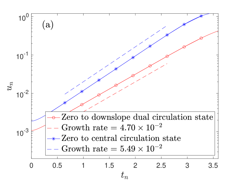
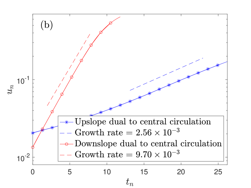
Figure 7: Comparison of initial growth of normalized $u$ velocity of simulation to growth rate predicted by LSA for (a) Zero state to the dual-circulation state at point $(0.36,0.36,0)$, and zero state to the central-circulation state at point $(0,0.9,0)$, and (b) Upslope dual-circulation state to central-circulation state, and downslope dual to central-circulation state both at point $(0,0.9,0)$. All cases at $\Pi_{s}=0.9$.

Comparing the possible transition scenarios from the zero-velocity base flow to the asymmetric steady state, it is worthwhile to point out a subtle yet significant distinction. In the first scenario when the original quiescent flow is perturbed by the central-circulation eigenmode (Figure 2a-b) which retains the mirror symmetry of the linearized governing equations, the flow eventually loses its initial symmetry (in this case, a $\mathcal{C}_{1}$-symmetry) due to nonlinear convection terms of the N-S equation, which gain significant strength once the initial perturbation grows to attain a non-negligible magnitude. In the second scenario, the flow is perturbed by the dual-circulation eigenmode (Figure 2c-d) and reaches the symmetric steady state without losing the symmetry of the initial perturbation in the process (in this case, a $\mathcal{C}_{2}$-symmetry), and only then the symmetry of this steady state is broken by its dominant instability mode that takes it to the asymmetric steady state. This describes the two possible paths by which the symmetry of the flow in the valley can be broken.

III.3 Bifurcation diagram

From our simulations, we now characterize the change in the possible steady-state profiles with a change in our $\Pi_{s}$ parameter. We observe two primary instabilities, each of which lead to two possible steady-state profiles. Therefore, each of these instabilities represents a supercritical pitchfork bifurcation, and we draw a bifurcation diagram, shown in Figure 8, where we plot the absolute maximum vorticity (positive or negative) in the $z$ direction multiplied by the sign of the maximum vertical velocity $v$ as a function of $\Pi_{s}$. The choice of maximum vorticity is based on the two asymmetric, central-circulation states in which the maximum vorticity is equal and opposite in sign in each case due to the dominant central circulation and the opposite direction of flow. However, this is not true of the upslope and downslope symmetric states. Both of these individual states consist of dual circulations in the valley with equal and opposite vorticity values. To resolve this in a way that illustrate the pitchfork bifurcation, we take the maximum positive vorticity value for each state and we multiply by the sign of the maximum vertical velocity $v$, which for the symmetric states occurs at the center of the valley and is opposite in sign. This creates the branching of the pitchfork bifurcation, with the negative branch representing the upslope steady state and the positive branch representing the downslope steady state. Because the two asymmetric states have exactly the same maximum vertical velocity value, this does not affect the outer branches at all.

In the bifurcation diagram, at low $\Pi_{s}$ values, the zero velocity state is linearly stable and is represented by the solid black line. At the first critical $\Pi_{s}$ value, estimated to be approximately 0.872, a pitchfork bifurcation occurs leading to the two possible asymmetric, central-circulation states. Both of these branches are linearly stable, and are thus represented by the solid blue lines. Because the clockwise and counterclockwise central-circulation states are mirror images of one another, each has equal and opposite maximum vorticity, and thus the branches of this pitchfork bifurcation are perfectly symmetric with respect to the $\omega_{z}=0$ axis, which is the form of a perfect pitchfork bifurcation. At slightly larger $\Pi_{s}$, an additional pitchfork bifurcation occurs from the unstable zero state, leading to the two possible dual-circulation states. The estimated critical $\Pi_{s}$ for this bifurcation is approximately 0.875. Because the dual-circulation states are unstable to a secondary central-circulation eigenmode, these branches are represented by dashed lines in the bifurcation diagram. The steady-state profiles for each of these unstable states was obtained through using the symmetric dual-circulation eigenmode as the initial conditions in the simulation, and minimizing sources of numerical error that could destabilize the symmetric profile (such as using high polynomial order, and using a structured, symmetric mesh).

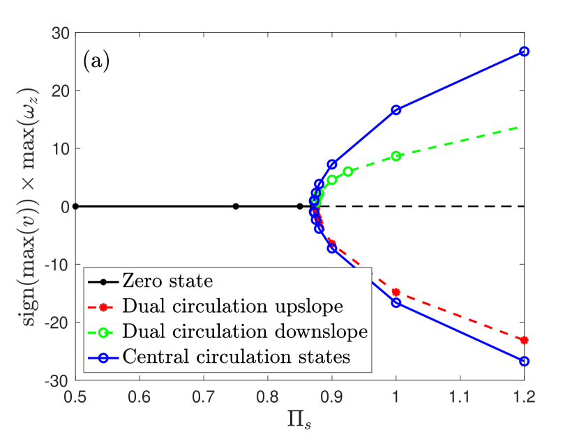
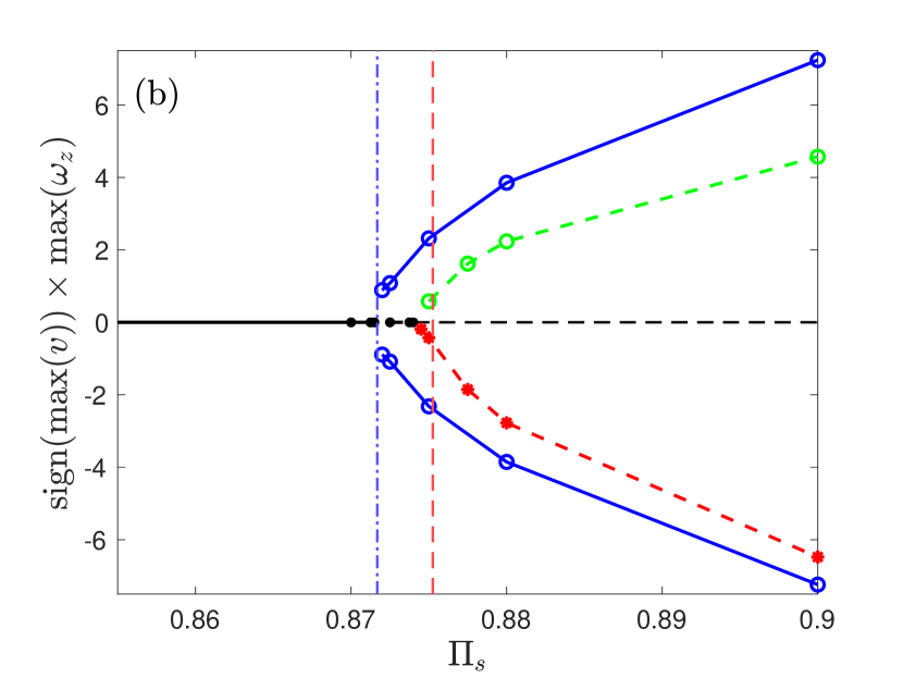
Figure 8: Bifurcation diagram for increasing $\Pi_{s}$. The quantity on the $y$-axis is the maximum normalized vorticity $\omega_{z}$ in the $z$ direction obtained from 3D N-S simulations, multiplied by the sign of the maximum vertical velocity. (a) shows the transition from the zero state to the asymmetric, central-circulation states and the symmetric, dual-circulation states. Note the asymmetry of the red and green curves with respect to $\omega_{z}=0$, (b) shows the same bifurcation plot zoomed into the critical value, along with critical values predicted by LSA shown as vertical lines.

However, we note that unlike the perfect pitchfork bifurcation diagram, with equal and opposite branches, because of the lack of any possible horizontal axis of symmetry in the valley geometry, the upslope and downslope branches differ in the magnitude of the vorticity at the same $\Pi_{s}$ value. In other words, the branches of this nested bifurcation are not symmetric to one another with respect to the $\omega_{z}=0$ axis. This can be most clearly seen comparing the red and green dashed curves in Figure 8a. This represents a perturbation, or an imperfection, to the pitchfork bifurcation which is caused by the lack of a horizontal axis of symmetry in our valley geometry. Imperfect pitchfork bifurcations have been observed in many fluid systems [31, 32, 33], as well as the coexistence of perfect and imperfect pitchfork bifurcations [34]. However, we note that our nested pitchfork bifurcation differs from many of these examples as well as the theory of imperfect pitchfork bifurcations [35] because it does not exhibit the separation of the branches at the critical point that is characteristic of imperfect pitchfork bifurcations. In the expected imperfect pitchfork bifurcation, the upper and lower branches detach at the critical point, and there is a smooth transition from the state prior to the bifurcation and one branch after the bifurcation. While we do not observe this behavior, we attribute this to the fact that our bifurcation occurs to the zero-velocity flow state, meaning a smooth transition to a non-zero flow state cannot occur. Therefore, while the inner, nested pitchfork bifurcation bears some resemblance to an imperfect pitchfork in its asymmetry, near the critical point, shown in more detail in Figure 8b, it more closely resembles a perfect pitchfork bifurcation.

A parallel can be drawn between our present findings and outcomes from a number of prior studies. One notable instance of an idealized geophysical model is the examination of thermohaline circulation within the ocean [19, 20]. It has been demonstrated by Welander [36] that straightforward box models depicting ocean circulation as a consequence of temperature and salinity disparities give rise to a minimum of four steady-state solutions, including two symmetric states and two asymmetric states, each characterized by opposing circulation directions. Additionally, the symmetrical configurations prove unstable to small perturbations, resulting in the emergence of asymmetric states wherein either the northern or southern circulation becomes dominant. This pattern holds true across all parameter values analyzed, mirroring the findings of the current study.

An additional example is the work of S. Yanase, J. Mizushima, and K. Araki [34], who studied the stability and steady states of flow between two concentric spheres with differential heating and rotation. Similar to the present study, they observed both asymmetric and symmetric solutions with respect to the equator, and they further classified the symmetric solutions into upward and downward configurations, which differ in their flow profile and heat transfer rates. This parallels the finding in the current study of a pair of asymmetric and symmetric solutions, with the symmetric solutions differing in flow profile due to the geometry of the given problem.

IV Conclusion

We examined the instabilities of stably stratified laminar flows within a valley-shaped enclosure heated from below with unique boundary conditions and a representation of ambient stratification in the governing equations, following the Prandtl model for slope flows. We performed linear stability analysis (LSA) as well as three-dimensional Navier-Stokes (N-S) simulations with 2D and 3D perturbations to validate our results. For a fixed slope angle and Prandtl number, the flow behavior is delineated by two dimensionless parameters: the stratification perturbation parameter $\Pi_{s}$, and $\Pi_{h}$, a new addition to the parameter space of stratified heated triangular cavities, and which is related to the buoyancy number employed in related studies [23]. In the results presented here, we focus only on the effect of the $\Pi_{s}$ parameter while keeping the remaining dimensionless parameters fixed. When $\Pi_{s}$ assumes very small values, indicative of subtle surface heating or very strong background stratification, a stable quiescent conduction state persists, for which we derive exact solutions for the pressure and buoyancy field.

Above a critical $\Pi_{s}$ value, two main instabilities come to the forefront as determined by LSA. One eigenmode reveals a single dominant circulation at the valley’s center, while the other displays two circulations of equivalent yet opposing intensity within the central valley region. The critical value for the central-circulation eigenmode is slightly lower than that for the dual-circulation eigenmode. We find that both eigenmodes are symmetric about the vertical axis, but each satisfies a different symmetry.

The dual-circulation eigenmode gives rise to two types of symmetrical steady-state profiles, where one features circulations containing upslope flow, and the other features downslope flow. While these states maintain the same reflection symmetry as the eigenmode, their dissimilarity results from the absence of any feasible symmetry about the $x$-axis within the valley geometry. The second type of instability, the central-circulation eigenmode, gives rise to a pair of asymmetric steady-state profiles, each characterized by either clockwise or counterclockwise dominant circulations in the valley-shaped enclosure. While the symmetry of the eigenmode is broken by the nonlinear evolution to the steady-state profiles, the clockwise and counterclockwise asymmetric states are perfect reflections of one another about the vertical axis.

The secondary stability analysis reveals that the symmetric, dual-circulation steady-state profiles are prone to further instability, leading to the emergence of the asymmetric steady state. This creates a unique bifurcation diagram with two nested, supercritical pitchfork bifurcations. The first pitchfork bifurcation, representing the asymmetric steady states, is a perfect pitchfork bifurcation, whereas the nested pitchfork bifurcation, representing the symmetric steady states, displays some imperfection in the asymmetry of the branches of the pitchfork bifurcation due to the difference between the upslope and downslope states. This nested bifurcation is fully unstable for all parameter values, and will transition to the stable asymmetric state under the slightest asymmetric perturbation.

The present study adds a number of important observations about the essential flow dynamics in stratified heated valley-shaped enclosures that have not been previously recognized. First, given our chosen boundary conditions combined with the presence of an ambient stratification, we have identified the existence of a quiescent, pure conduction state which is stable with very low surface heating or very large stratification. With the discovery of this quiescent base state, we are able to characterize the complete flow behavior within the parameter space through the use of LSA and nonlinear N-S simulations, which reveal five possible equilibrium states, as depicted at the larger $\Pi_{s}$ values in the bifurcation diagram. This characterization also reveals the existence of the counter-intuitive downslope, symmetric flow state, another previously unidentified flow state in heated, stratified valleys. While this downslope state is inherently unstable, our use of LSA along with careful initial conditions in 3D N-S simulations enables us to identify that this is an additional possible steady state solution. Another important finding in the current study is the instability of the symmetric steady state and precedence of the asymmetric steady state over the symmetric state. Prior studies of flows in heated, triangular cavities suggest that the symmetric, dual-circulation state is the base state which only transitions to the asymmetric state after a pitchfork bifurcation occurs [10, 13]. In contrast, under the current configuration, we find the base state can be a quiescent, steady, pure conduction state. With this base state, the asymmetric state manifests in the valley-shaped enclosure as a result of the primary instability, with a larger growth rate and lower critical $\Pi_{s}$ value in comparison to the symmetric state. In addition, we find the symmetric state to be unstable at all parameter values considered here. This observation is important because, for a random perturbation to the quiescent base flow, we would only expect to obtain asymmetric steady-state profiles, and not the symmetric dual-circulation state. We confirmed this expectation through 3D Navier-Stokes simulations with random initial conditions for $L_{z}$ between 2 and 16 at $\Pi_{s}=0.9$, all of which are observed to converge to the asymmetric steady state.

Our findings reveal that the combination of linear stability analysis and nonlinear flow simulations can be an effective and precise approach for analyzing the dynamics of steady laminar flows within a stably stratified, heated valley-shaped enclosure. Within this context, we have demonstrated that, for a given set of dimensionless parameters, the Navier-Stokes equations admit at least five unique solutions, including symmetric and asymmetric convection patterns and an additional quiescent, pure conduction state. However, the asymmetric state is stable at all parameter values investigated here whereas the symmetric state is unstable, suggesting a higher likelihood of observation of the asymmetric state in natural settings. This phenomenon is anticipated to be even more pronounced when considering the inherent asymmetry and heterogeneity present in real valleys.

References

- Holtslag et al. [2013] A. A. M. Holtslag, G. Svensson, P. Baas, S. Basu, B. Beare, A. C. M. Beljaars, F. C. Bosveld, J. Cuxart, J. Lindvall, G. J. Steeneveld, et al., Stable atmospheric boundary layers and diurnal cycles: challenges for weather and climate models, Bull. Amer. Meteor. 94, 1691 (2013).
- Angevine et al. [2020] W. M. Angevine, J. M. Edwards, M. Lothon, M. A. LeMone, and S. R. Osborne, Transition periods in the diurnally-varying atmospheric boundary layer over land, Boundary-Layer Meteorol. 177, 205 (2020).
- Boutle et al. [2018] I. Boutle, J. Price, I. Kudzotsa, H. Kokkola, and S. Romakkaniemi, Aerosol–fog interaction and the transition to well-mixed radiation fog, Atmos. Chem. Phys. 18, 7827 (2018).
- Salmond and McKendry [2005] J. A. Salmond and I. G. McKendry, A review of turbulence in the very stable nocturnal boundary layer and its implications for air quality, Prog. Phys. Geogr. 29, 171 (2005).
- Prandtl [1942] L. Prandtl, Führer durch die Strömungslehre (Vieweg und Sohn, 1942).
- Prandtl [1953] L. Prandtl, Essentials of Fluid Dynamics: With Applications to Hydraulics, Aeronautics, Meteorology and other Subjects (Blackie & Son, 1953).
- Princevac and Fernando [2008] M. Princevac and H. J. S. Fernando, Morning breakup of cold pools in complex terrain, J. Fluid Mech. 616, 99 (2008).
- Wang et al. [2021] X. Wang, S. Bhowmick, Z. F. Tian, S. C. Saha, and F. Xu, Experimental study of natural convection in a V-shape-section cavity, Phys. Fluids 33, 014104 (2021).
- Saha and Khan [2011] S. C. Saha and M. M. K. Khan, A review of natural convection and heat transfer in attic-shaped space, Energy Build. 43, 2564 (2011).
- Ridouane and Campo [2006] E. H. Ridouane and A. Campo, Formation of a pitchfork bifurcation in thermal convection flow inside an isosceles triangular cavity, Phys. Fluids 18, 074102 (2006).
- Omri et al. [2007] A. Omri, M. Najjari, and S. B. Nasrallah, Numerical analysis of natural buoyancy-induced regimes in isosceles triangular cavities, Numerical Heat Transfer, Part A: Applications 52, 661 (2007).
- Holtzman et al. [2000] G. A. Holtzman, R. W. Hill, and K. S. Ball, Laminar natural convection in isosceles triangular enclosures heated from below and symmetrically cooled from above, J. Heat Transfer 122, 485 (2000).
- Bhowmick et al. [2018] S. Bhowmick, F. Xu, X. Zhang, and S. C. Saha, Natural convection and heat transfer in a valley shaped cavity filled with initially stratified water, Int. J. Therm. Sci. 128, 59 (2018).
- Bhowmick et al. [2019] S. Bhowmick, S. C. Saha, M. Qiao, and F. Xu, Transition to a chaotic flow in a v-shaped triangular cavity heated from below, Int. J. Heat Mass Transf. 128, 76 (2019).
- Bhowmick et al. [2022] S. Bhowmick, F. Xu, M. M. Molla, and S. C. Saha, Chaotic phenomena of natural convection for water in a v-shaped enclosure, Int. J. Therm. Sci. 176, 107526 (2022).
- Gelfgat et al. [1999] A. Y. Gelfgat, P. Z. Bar-Yoseph, and A. L. Yarin, Stability of multiple steady states of convection in laterally heated cavities, J. Fluid Mech. 388, 315 (1999).
- Erenburg et al. [2003] V. Erenburg, A. Y. Gelfgat, E. Kit, P. Z. Bar-Yoseph, and A. Solan, Multiple states, stability and bifurcations of natural convection in a rectangular cavity with partially heated vertical walls, J. Fluid Mech. 492, 63 (2003).
- Venturi et al. [2010] D. Venturi, X. Wan, and G. E. Karniadakis, Stochastic bifurcation analysis of Rayleigh–Bénard convection, J. Fluid Mech. 650, 391 (2010).
- Marotzke et al. [1988] J. Marotzke, P. Welander, and J. Willebrand, Instability and multiple steady states in a meridional-plane model of the thermohaline circulation, Tellus A: Dyn. Meteorol. Oceanogr. 40, 162 (1988).
- Bryan [1986] F. Bryan, High-latitude salinity effects and interhemispheric thermohaline circulations, Nature 323, 301 (1986).
- Xiao and Senocak [2019] C. Xiao and I. Senocak, Stability of the Prandtl model for katabatic slope flows, J. Fluid Mech. 865 (2019).
- Xiao and Senocak [2020] C. Xiao and I. Senocak, Stability of the anabatic Prandtl slope flow in a stably stratified medium, J. Fluid Mech. 885 (2020).
- J. Yalim, J. M. Lopez, and B. D. Welfert [2018] J. Yalim, J. M. Lopez, and B. D. Welfert, Vertically forced stably stratified cavity flow: instabilities of the basic state, J. Fluid Mech. 851, R6 (2018).
- Grayer et al. [2020] H. Grayer, J. Yalim, B. D. Welfert, and J. M. Lopez, Dynamics in a stably stratified tilted square cavity, J. Fluid Mech. 883 (2020).
- Shir and Joseph [1968] C. Shir and D. Joseph, Convective instability in a temperature and concentration field, Arch. Rational Mech. Anal 30, 38 (1968).
- Xiao and Senocak [2022] C. Xiao and I. Senocak, Impact of stratification mechanisms on turbulent characteristics of stable open-channel flows, J. Atmos. Sci. 79, 205 (2022).
- Cantwell et al. [2015] C. D. Cantwell, D. Moxey, A. Comerford, A. Bolis, G. Rocco, G. Mengaldo, D. De Grazia, S. Yakovlev, J.-E. Lombard, D. Ekelschot, et al., Nektar++: An open-source spectral/hp element framework, Comput. Phys. Commun. 192, 205 (2015).
- Moxey et al. [2020] D. Moxey, C. D. Cantwell, Y. Bao, A. Cassinelli, G. Castiglioni, S. Chun, E. Juda, E. Kazemi, K. Lackhove, J. Marcon, et al., Nektar++: Enhancing the capability and application of high-fidelity spectral/hp element methods, Comput. Phys. Commun. 249, 107110 (2020).
- Moffatt [1964] H. K. Moffatt, Viscous and resistive eddies near a sharp corner, J. Fluid Mech. 18, 1 (1964).
- [30] See supplemental material [url] for animation of transition from central circulation eigenvector to asymmetric steady state.
- Benjamin [1978] T. B. Benjamin, Bifurcation phenomena in steady flows of a viscous fluid. I. Theory, Proc. R. Soc. A: Math. Phys. Eng. Sci. 359, 1 (1978).
- M. Alam, V. H. Arakeri, P. R. Nott, J. D. Goddard, and H. J. Herrmann [2005] M. Alam, V. H. Arakeri, P. R. Nott, J. D. Goddard, and H. J. Herrmann, Instability-induced ordering, universal unfolding and the role of gravity in granular couette flow, J. Fluid Mech. 523, 277 (2005).
- O. Cadot, A. Evrard, and L. Pastur [2015] O. Cadot, A. Evrard, and L. Pastur, Imperfect supercritical bifurcation in a three-dimensional turbulent wake, Phys. Rev. E 91, 063005 (2015).
- S. Yanase, J. Mizushima, and K. Araki [1995] S. Yanase, J. Mizushima, and K. Araki, Multiple solutions for a flow between two concentric spheres with different temperatures and their stability, J. Phys. Soc. Japan 64, 2433 (1995).
- M. Golubitsky and D. G. Schaeffer [1985] M. Golubitsky and D. G. Schaeffer, Singularities and Groups in Bifurcation Theory, Vol. 1 (Springer, 1985).
- Welander [1986] P. Welander, Thermohaline effects in the ocean circulation and related simple models, in Large-scale transport processes in oceans and atmosphere (Springer, 1986) pp. 163–200.