Testing for linearity in scalar-on-function regression
with responses missing at random

Abstract

We construct a goodness-of-fit test for the Functional Linear Model with Scalar Response (FLMSR) with responses Missing At Random (MAR). For that, we extend an existing testing procedure for the case where all responses have been observed to the case where the responses are MAR. The testing procedure gives rise to a statistic based on a marked empirical process indexed by the randomly projected functional covariate. The test statistic depends on a suitable estimator of the functional slope of the FLMSR when the sample has MAR responses, so several estimators are proposed and compared. With any of them, the test statistic is relatively easy to compute and its distribution under the null hypothesis is simple to calibrate based on a wild bootstrap procedure. The behavior of the resulting testing procedure as a function of the estimators of the functional slope of the FLMSR is illustrated by means of several Monte Carlo experiments. Additionally, the testing procedure is applied to a real data set to check whether the linear hypothesis holds.

Keywords: Functional linear model; Functional principal components; Goodness-of-fit tests; Marked empirical processes; Missing at random; Wild bootstrap.

1 Introduction

Functional Data Analysis (FDA) is a field of statistics that analyzes random variables that are observed throughout a continuum, typically in the form of random functions. Ramsay and Silverman, (2005), Ferraty and Vieu, (2006), Horváth and Kokoszka, (2012), Hsing and Eubank, (2015), and Kokoszka and Reimherr, (2017) are comprehensive introductions to the field from several points of view. In particular, one of the most important issues in FDA is to analyze regression models in which the response and/or the covariates has/have a functional nature, see, for instance, the surveys by Febrero-Bande et al., (2017) and Reiss et al., (2017), who focused on estimation methods when there is a functional covariate and a scalar response, and Greven and Scheipl, (2017), who proposed a general framework for additive (mixed) models for functional covariates and/or functional responses. One of the most widely studied situations involves a real response variable, $Y$, and a functional covariate, $\mathcal{X}$, so it is appropriate to describe the relationship between them through a regression model with random design given by $Y=m\left(\mathcal{X}\right)+\varepsilon$, where $m\left({\scriptstyle\mathcal{X}}\right)=\mathbb{E}\left[Y|\mathcal{X}={\scriptstyle\mathcal{X}}\right]$ is the regression function of $Y$ on $\mathcal{X}$ and $\varepsilon$ is an error random variable with zero mean, finite variance $\sigma_{\varepsilon}^{2}$, and uncorrelated with $\mathcal{X}$. When a random sample $\{\left(\mathcal{X}_{i},Y_{i}\right)\}_{i=1}^{n}$ from the pair $\left(\mathcal{X},Y\right)$ is available, it is of interest to check whether the regression function $m$ is linear since this is, conceptually, the simplest non-trivial parametric structure for $m$. For that, García-Portugués et al., (2014) proposed a goodness-of-fit test based on a Cramér–von Mises-like norm that integrates, for a set of functional directions, the marked empirical processes indexed by the projected functional covariate on each of the directions. The resulting test is somehow computationally-intensive and this is one of the driving motivations in Cuesta-Albertos et al., (2019) for considering the aforementioned empirical process but for a collection of randomly-chosen directions. Goodness-of-fit tests for the functional linear model follow by applying norms over the processes associated with each random direction, with posterior aggregation of the different $p$-values by means of the false discovery rate method. The projection-based procedure is computationally less expensive than the Cramér–von Mises-like procedure, although at the cost of some loss in power. Also in the scalar-on-function regression type models, although in a different setting, McLean et al., (2015) proposed a restricted likelihood ratio test for testing linearity within the class of functional generalized additive models. The goodness-of-fit test based on a Cramér–von Mises-like norm has been extended to the case with functional response in García-Portugués et al., (2020). González-Manteiga et al., (2023) and González-Manteiga, (2023) provide reviews of goodness-of-fit advances for regression models involving functional data.

In certain circumstances, the observed random sample contains responses that are Missing At Random (MAR). For instance, Febrero-Bande et al., (2019) considered mean curves of the annual average daily temperature in weather stations to predict the corresponding average of the total number of sunny days per year. The responses contained missing values due to the unavailability of recordings for the presence of opaque clouds in certain weather stations. Then, these authors proposed two methods for estimating the functional slope of the Functional Linear Model with Scalar Response (FLMSR), both for imputing the missing responses and for predicting new responses. The first one is the simplified method: it estimates the functional slope by using only the pairs of covariates and responses that are observed and afterward employs the estimated functional slope to impute missing responses and to predict new responses. On top of that, the imputed method, re-estimates the functional slope, using both the complete pairs and the pairs with responses imputed by the simplified method, and this re-estimate is posteriorly employed to impute missing responses and to predict new responses. Crambes and Henchiri, (2019) have analyzed asymptotic properties of the simplified method, obtaining mean square error rates for the imputed values resulting from the simplified functional slope estimate. In a different setting, when the regression function operator is unspecified, Ferraty et al., (2013) and Ling et al., (2016) focused on estimating the unconditional mean and the conditional mode of the response, respectively, when some of the responses are MAR, Ling et al., (2015) developed a nonparametric method to estimate the unspecified regression function operator under MAR responses and Ling et al., (2022) investigated the estimation of the functional single index regression model with missing responses at random for strong mixing time series data. Ciarleglio et al., (2022) related through functional regression certain brain measures derived from electroencephalography containing missing observations and proposed several imputation methods. Beyond FDA, the MAR situation has been thoroughly studied in multiple linear regression; see, among others, González-Manteiga and Pérez-González, (2006), Sun and Wang, (2009), Li, (2012), Sun et al., (2017), Zheng et al., (2020), Pérez González et al., (2021), and references therein.

The main goal of this article is to develop a testing procedure for checking whether the regression function $m$ is linear and, consequently, an FLMSR is suitable to explain the relationship between the functional covariate $\mathcal{X}$ and the scalar response $Y$, when some of the responses are MAR. For that, we extend the testing procedure proposed in García-Portugués et al., (2014) because, although less computationally efficient, it is more powerful than the procedure in Cuesta-Albertos et al., (2019). Moreover, note that a data set with MAR responses has some limited information, so it seems convenient to gain some power to compensate for the lack of information, at the cost of losing some computational efficiency. The proposed testing procedure relies on a statistic constructed from a marked empirical process based on residuals. These residuals are those obtained after estimating the functional slope with some appropriate method under MAR responses. Therefore, we consider and compare empirically six different estimators to determine which one is the most appropriate for the proposed testing procedure. As in the case of fully observed responses, the distribution of the statistic associated with the testing procedure is calibrated by means of wild bootstrap resampling on the corresponding residuals.

The rest of this paper is structured as follows. Section 2 presents the testing problem and the main assumptions when the scalar response is MAR. Section 3 presents six estimators of the functional slope of the FLMSR when there are missing responses that are suitable to perform the linearity test under the MAR hypothesis. Section 4 presents the testing procedure in conjunction with the marked empirical process and implements the wild bootstrap resampling strategy. Section 5 illustrates the performance of the testing procedure in several simulation experiments. Section 6 presents the results of applying the testing procedure for checking whether the linear hypothesis holds when predicting the average of the total number of sunny days per year by means of the mean curves of the annual average daily temperature in a set of weather stations in Spain. Finally, Section 7 summarizes some concluding remarks.

2 The testing problem

Let $\mathbb{H}$ be a real separable Hilbert space endowed with the inner product $\langle\cdot,\cdot\rangle$ and its associated norm $\|\cdot\|_{\mathbb{H}}$. While $\mathbb{H}$ is a general real separable Hilbert space, the most frequent assumption in the literature is that $\mathbb{H}$ is the $L^{2}\left[a,b\right]$ space defined as the set of all functions $\eta:\left[a,b\right]\rightarrow\mathbb{R}$ such that $\|\eta\|_{2}:=\langle\eta,\eta\rangle^{1/2}$ is finite, where the inner product of two functions $\eta,\varphi\in L^{2}\left[a,b\right]$ is defined as $\langle\eta,\varphi\rangle:=\int_{a}^{b}\eta\left(t\right)\varphi\left(t\right)\,\mathrm{d}t$. Furthermore, let $\mathcal{X}$ be a functional random variable belonging to $\mathbb{H}$ with zero-mean function and covariance operator $\Gamma$ defined as

$$\Gamma\left[\eta\right]:=\mathbb{E}\left[\left(\mathcal{X}\otimes\mathcal{X}\right)\left(\eta\right)\right]:=\mathbb{E}\left[\left\langle\mathcal{X},\eta\right\rangle\mathcal{X}\right],\quad\text{for any $\eta\in\mathbb{H}$.}$$ (1)

The covariance operator $\Gamma$ in (1) is assumed to have a sequence of positive eigenvalues $a_{1}>a_{2}>\cdots$ with multiplicity one, associated with a set of orthonormal eigenfunctions, denoted by $\psi_{1},\psi_{2},\ldots$, such that $\Gamma\left[\psi_{k}\right]=a_{k}\psi_{k}$, for $k\in\mathbb{N}$.

Additionally, it is assumed that the functional random variable $\mathcal{X}$ is related to a zero-mean real random variable $Y$, defined in the same probability space, through a regression model with random design given by $Y=m\left(\mathcal{X}\right)+\varepsilon$, where $m:{\scriptstyle\mathcal{X}}\in\mathbb{H}\mapsto\mathbb{E}\left[Y|\mathcal{X}={\scriptstyle\mathcal{X}}\right]\in\mathbb{R}$ is the regression function of $Y$ over $\mathcal{X}$ and $\varepsilon$ is a zero-mean random variable with finite variance $\sigma_{\varepsilon}^{2}$ and uncorrelated with $\mathcal{X}$. In addition, we consider a scalar response $Y$ that has some potential missingness, as described later in (5). Within this setting, the goal is to test the composite hypothesis

$$H_{0}:m\in\mathcal{L}:=\left\{\langle\cdot,\beta\rangle:\beta\in\mathbb{H}\right\}$$ (2)

versus the general alternative hypothesis

$$H_{1}:m\not\in\mathcal{L}:=\left\{\langle\cdot,\beta\rangle:\beta\in\mathbb{H}\right\}.$$ (3)

Thus, if the null hypothesis (2) holds, the relationship between the functional covariate $\mathcal{X}$ and the real response $Y$ is driven by the FLMSR given by

$$Y=\left\langle\mathcal{X},\beta\right\rangle+\varepsilon,$$ (4)

where $\beta\in\mathbb{H}$ is the unspecified functional slope of the model, whose existence and uniqueness are ensured, as shown in Cardot et al., (2007), under the following two fundamental assumptions:

1. $\mathcal{X}$ and $Y$ satisfy $\sum\limits_{k=1}^{\infty}\frac{1}{a_{k}^{2}}\left\langle\mathbb{E}\left[Y\mathcal{X}\right],\psi_{k}\right\rangle^{2}<\infty$.

2. $\mathrm{Ker}\left(\Gamma\right)=\left\{0\right\}$.

Now, to test the null hypothesis (2) versus the alternative hypothesis (3), it is assumed that we have a random independent and identically distributed (iid) sample $\left\{\left(\mathcal{X}_{i},Y_{i},R_{i}\right)\right\}_{i=1}^{n}$ generated from the triplet $\left(\mathcal{X},Y,R\right)$, where $R$ is a Bernoulli variable that acts as an indicator of the missing responses, such that $R_{i}=1$ if $Y_{i}$ is observed and $R_{i}=0$ if $Y_{i}$ is missing, for $i=1,\ldots,n$. More precisely, it is assumed that the missing mechanism is MAR, with observance probability driven by

$$\mathbb{P}\left(R=1|Y,\mathcal{X}\right)=\mathbb{P}\left(R=1|\mathcal{X}\right)=:p\left(\mathcal{X}\right),$$ (5)

where $p:\mathbb{H}\rightarrow[0,1]$ is an unspecified function operator of $\mathcal{X}$ that describes the missing probability for $Y$. Hence, the real response $Y$ and the indicator variable $R$ are conditionally independent given the functional covariate $\mathcal{X}$, a common and realistic mechanism that allows missing responses to be predicted with the available information. If (5) does not hold, then the values of the missing responses cannot be adequately predicted as they depend on information that is not available.

3 Parameter estimation of the FLMSR with MAR responses

The MAR-adapted procedure presented in Section 4 for testing (2) relies on a suitable estimate of the functional slope $\beta$ of the FLMSR (4) and the residuals associated with this estimation. Thus, initially, we briefly summarize the simplified and imputed estimators proposed in Febrero-Bande et al., (2019) and then propose the inverse probability weighted estimator which, contrary to the previous ones, takes into account the mechanism of generation of missing responses in (5). Moreover, following García-Portugués et al., (2020), we subsequently present the simplified, imputed, and inverse probability weighted MAR-adapted LASSO-selected estimators, which use LASSO as an alternative to the use of least squares and cross-validation for the estimation of the FLMSR, as done in Febrero-Bande et al., (2019). In this way, we will have an array of different estimators that we will compare in Section 5.

For all this, it is helpful to write the FLMSR (4) in a simpler way. Under the assumptions given in Section 2, the functional random variable $\mathcal{X}$ and the functional slope $\beta$ can be represented in terms of the eigenfunctions of the covariance operator $\Gamma$ in (1), as follows

$$\mathcal{X}=\sum\limits_{k=1}^{\infty}S_{k}\psi_{k},\qquad\beta=\sum\limits_{k=1}^{\infty}b_{k}\psi_{k},$$ (6)

where $S_{k}:=\left\langle\mathcal{X},\psi_{k}\right\rangle$, $k\in\mathbb{N}$, are the Functional Principal Component (FPC) scores, that are uncorrelated random variables with $\mathbb{E}\left[S_{k}\right]=0$ and $\mathbb{V}\mathrm{ar}\left[S_{k}\right]=a_{k}$, and $b_{k}:=\left\langle\beta,\psi_{k}\right\rangle$, $k\in\mathbb{N}$, are deterministic coefficients. Hence, the FLMSR (4) can be written as an infinite linear combination of the FPC scores, resulting in

$$Y=\sum\limits_{k=1}^{\infty}b_{k}S_{k}+\varepsilon.$$ (7)

The expression (7) allows $\beta$ to be estimated in different ways, see Cardot et al., (2007) when the random sample only contains complete pairs of covariates and responses, and Febrero-Bande et al., (2019) when the random sample contains MAR responses. In summary, all these ways boil down to three fundamental steps: (i) truncate the series (6) and (7) up to $K_{n}\leq n$, where $K_{n}$ possibly depends on the sample; (ii) plug-in estimates $\big{\{}\widehat{\psi}_{k}\big{\}}_{k=1}^{K_{n}}$ of $\big{\{}\psi_{k}\big{\}}_{k=1}^{K_{n}}$ in $S_{k}$; and (iii) fit the resultant linear model. More precisely, whether the responses are missing or not, the covariance operator $\Gamma$ in (1) is estimated with the sample covariance operator of the complete set of covariates $\left\{\mathcal{X}_{i}\right\}_{i=1}^{n}$ defined as

$$\widehat{\Gamma}\left[\eta\right]:=\frac{1}{n}\sum\limits_{i=1}^{n}\left\langle\mathcal{X}_{i},\eta\right\rangle\mathcal{X}_{i},\quad\text{for any $\eta\in\mathbb{H}$,}$$ (8)

that has a sequence of nonnegative eigenvalues, denoted by $\widehat{a}_{1}\geq\widehat{a}_{2}\geq\cdots\geq 0$, with $\widehat{a}_{k}=0$, for $k>n$, and a set of orthonormal eigenfunctions, denoted by $\widehat{\psi}_{1},\widehat{\psi}_{2},\ldots$ such that $\widehat{\Gamma}\big{[}\widehat{\psi}_{k}\big{]}=\widehat{a}_{k}\widehat{\psi}_{k}$, for $k=1,2,\ldots$ The eigenfunctions $\widehat{\psi}_{1},\widehat{\psi}_{2},\ldots$ allow the sample FPC scores to be defined as $\widehat{S}_{i,k}:=\big{\langle}\mathcal{X}_{i},\widehat{\psi}_{k}\big{\rangle}$, for $i=1,\ldots,n$ and $k=1,\ldots,K_{n}$, giving rise to the resultant linear model associated with (7):

$$Y_{i}=\sum\limits_{k=1}^{K_{n}}b_{k}\widehat{S}_{i,k}+\varepsilon_{i},\quad\text{for $i=1,\ldots,n$.}$$ (9)

When there are MAR responses, Febrero-Bande et al., (2019) proposed, firstly, the simplified estimation method that follows the naive idea of using only pairs responses and FPC scores with observed responses to estimate $\{b_{k}\}_{k=1}^{K_{n}}$ in (9). More precisely, if $i_{\mathcal{S}}:=\left\{i:R_{i}=1\right\}_{i=1}^{n}$, i.e., the set of indices of the observed responses, the simplified estimator of $\beta$ is given by

$$\widehat{\beta}_{\mathcal{S}}:=\sum\limits_{k=1}^{K_{\mathcal{S}}}\widehat{b}_{k,\mathcal{S}}\widehat{\psi}_{k},$$ (10)

where $\widehat{b}_{1,\mathcal{S}},\ldots,\widehat{b}_{K_{\mathcal{S}},\mathcal{S}}$ are the Ordinary Least Squares (OLS) estimates of $b_{1},\ldots,b_{K_{\mathcal{S}}}$, i.e.,

$$\widehat{b}_{k,\mathcal{S}}:=\frac{1}{n_{\mathcal{S}}\widehat{a}_{k}}\sum\limits_{i\in i_{\mathcal{S}}}Y_{i}\widehat{S}_{i,k},\quad\text{for $k=1,\ldots,K_{\mathcal{S}}$}.$$

Above, $n_{\mathcal{S}}:=\#\left\{i_{\mathcal{S}}\right\}$ is the number of indices in $i_{\mathcal{S}}$, and $K_{\mathcal{S}}$ is a certain cutoff selected from the set $\left\{1,\ldots,K_{\max}\right\}$ by leave-one-out cross-validation, where $K_{\max}\leq n$ is a certain upper bound. Alternatives to cross-validation like model selection criteria such as the Bayesian Information Criterion (BIC) or Generalized Cross-Validation (GCV) depend on the likelihood function and/or the degrees of freedom parameter, which are not immediately determined for the FLMSR with MAR responses. Secondly, Febrero-Bande et al., (2019) proposed the imputed estimation method that imputes missing responses with the simplified estimator $\widehat{\beta}_{\mathcal{S}}$ in (10) to subsequently estimate $\{b_{k}\}_{k=1}^{K_{n}}$ in (9) with all pairs of responses and FPC scores, whether responses are observed or imputed. To impute, we use the equality $\mathbb{E}\left[RY+\left(1-R\right)\left\langle\mathcal{X},\beta\right\rangle\right]=\mathbb{E}\left[Y\right]$, similar to the one used in Sun and Wang, (2009) and Sun et al., (2017), among others, in multiple linear regression models. This equality justifies the use of the completed sample $\left\{\left(\mathcal{X}_{i},Y_{i,\mathcal{S}},R_{i}\right)\right\}_{i=1}^{n}$, where $Y_{i,\mathcal{S}}=R_{i}Y_{i}+\left(1-R_{i}\right)\big{\langle}\mathcal{X}_{i},\widehat{\beta}_{\mathcal{S}}\big{\rangle}$, for $i=1,\ldots,n$, to estimate $\beta$. Then, the imputed estimator of $\beta$ is defined as

$$\widehat{\beta}_{\mathcal{I}}:=\sum\limits_{k=1}^{K_{\mathcal{I}}}\widehat{b}_{k,\mathcal{I}}\widehat{\psi}_{k},$$ (11)

where $K_{\mathcal{I}}$ is a certain cutoff and $\widehat{b}_{1,\mathcal{I}},\ldots,\widehat{b}_{K_{\mathcal{I}},\mathcal{I}}$ are the OLS estimates of $b_{1},\ldots,b_{K_{\mathcal{I}}}$ given by

$$\widehat{b}_{k,\mathcal{I}}:=\frac{1}{n\widehat{a}_{k}}\sum\limits_{i=1}^{n}Y_{i,\mathcal{S}}\widehat{S}_{i,k},\quad\text{for $k=1,\ldots,K_{\mathcal{I}}$},$$

where the cutoffs $\left(K_{\mathcal{S}},K_{\mathcal{I}}\right)$ are selected from the set $\left\{1,\ldots,K_{\max}\right\}\times\left\{1,\ldots,K_{\max}\right\}$ by means of a double leave-one-out cross-validation procedure. Importantly, the cutoff $K_{\mathcal{S}}$ selected for the simplified estimator $\widehat{\beta}_{\mathcal{S}}$ in (10) does not have to equal the cutoff $K_{\mathcal{S}}$ selected for the imputed estimator $\widehat{\beta}_{\mathcal{I}}$ in (11). Using these two cutoffs, Febrero-Bande et al., (2019) illustrated that $\widehat{\beta}_{\mathcal{I}}$ in (11) can have a lower mean square error of estimation than $\widehat{\beta}_{\mathcal{S}}$ in (10) if the cutoffs $\left(K_{\mathcal{S}},K_{\mathcal{I}}\right)$ of the former estimator are selected appropriately. Alternatively, to impute missing responses, we also use the equality $\mathbb{E}\left[\left(R/p\left(\mathcal{X}\right)\right)Y+\left(1-R/p\left(\mathcal{X}\right)\right)\big{\langle}\mathcal{X},\beta\big{\rangle}\right]=\mathbb{E}\left[Y\right]$, where $p\left(\cdot\right)$ is the missing response operator (5), which is similar to the one used in Sun and Wang, (2009), Sun et al., (2017), Qin et al., (2017), Bianco et al., (2019), and Bianco et al., (2020), among others, in multiple linear regression models. This equality justifies the completed sample given by $\left\{\left(\mathcal{X}_{i},Y_{i,\mathcal{W}},R_{i}\right)\right\}_{i=1}^{n}$, where $Y_{i,\mathcal{W}}=\left(R_{i}/\widehat{p}\left(\mathcal{X}_{i}\right)\right)Y_{i}+\left(1-R_{i}/\widehat{p}\left(\mathcal{X}_{i}\right)\right)\big{\langle}\mathcal{X}_{i},\widehat{\beta}_{\mathcal{S}}\big{\rangle}$ for $i=1,\ldots,n$, and $\widehat{p}\left(\cdot\right)$ is the local constant Nadaraya–Watson estimator of the MAR mechanism $p\left(\cdot\right)$, given by

$$\widehat{p}\left({\scriptstyle\mathcal{X}}\right):=\sum_{i=1}^{n}\frac{K_{h}\left(\left\|{\scriptstyle\mathcal{X}}-\mathcal{X}_{i}\right\|_{\mathbb{H}}\right)}{\sum_{l=1}^{n}K_{h}\left(\left\|{\scriptstyle\mathcal{X}}-\mathcal{X}_{l}\right\|_{\mathbb{H}}\right)}R_{i}.$$ (12)

Above, $K_{h}\left(\cdot\right):=K\left(\cdot/h\right)/h$, $K:\left[0,\infty\right)\to\left[0,\infty\right)$ is a nonnegative kernel, and $h$ is a bandwidth that can be chosen by cross-validation. Then, the inverse probability weighted estimator of $\beta$ is defined as

$$\widehat{\beta}_{\mathcal{W}}:=\sum\limits_{k=1}^{K_{\mathcal{W}}}\widehat{b}_{k,\mathcal{W}}\widehat{\psi}_{k},$$ (13)

where $K_{\mathcal{W}}$ is a certain cutoff and $\widehat{b}_{1,\mathcal{W}},\ldots,\widehat{b}_{K_{\mathcal{W}},\mathcal{W}}$ are the OLS estimates of $b_{1},\ldots,b_{K_{\mathcal{W}}}$ given by

$$\widehat{b}_{k,\mathcal{W}}:=\frac{1}{n\widehat{a}_{k}}\sum\limits_{i=1}^{n}Y_{i,\mathcal{W}}\widehat{S}_{i,k},\quad\text{for $k=1,\ldots,K_{\mathcal{W}}$},$$

where the cutoffs $\left(K_{\mathcal{S}},K_{\mathcal{W}}\right)$ are selected similarly as the imputed estimator cutoffs are selected.

When all covariates and responses are observed, García-Portugués et al., (2020) proposed a LASSO-selected estimator of $\beta$ that uses LASSO to simultaneously estimate the coefficients $b_{k}$ and select significant FPC scores in (9). Therefore, to have a larger number of competitive estimators, we next present the simplified, imputed and inverse probability weighted MAR-adapted LASSO-selected estimators of $\beta$. Firstly, we carry out LASSO-type regression in $\big{\{}\big{(}Y_{i},\widehat{S}_{i,k}\big{)}:i\in i_{\mathcal{S}}\big{\}}$ to obtain

$$\big{(}\widetilde{b}_{1,\mathcal{SL}},\ldots,\widetilde{b}_{K_{\max},\mathcal{SL}}\big{)}^{\prime}=\underset{b_{1},\ldots,b_{K_{\max}}\in\mathbb{R}^{K_{\max}}}{\arg\min}\left\{\sum\limits_{i\in i_{\mathcal{S}}}\left(Y_{i}-\sum\limits_{k=1}^{K_{\max}}b_{k}\widehat{S}_{i,k}\right)^{2}+\lambda\sum_{k=1}^{K_{\max}}\left|b_{k}\right|\right\}$$ (14)

where $\lambda\geq 0$ is the penalty parameter that can be efficiently selected through the so-called one standard error rule, see Friedman et al., (2010), that as noted in García-Portugués et al., (2020) has certain advantages over the usual cross-validation rule. Then, as in García-Portugués et al., (2020), we re-estimate the coefficients $b_{k}$ selected by LASSO, using least squares to reduce the mean square error of the estimation. Therefore, the simplified MAR-adapted LASSO-selected estimator of $\beta$ is defined as

$$\widehat{\beta}_{\mathcal{SL}}:=\sum\limits_{k\in\mathcal{K}_{\mathcal{SL}}}\widehat{b}_{k,\mathcal{SL}}\widehat{\psi}_{k},$$ (15)

where $\mathcal{K}_{\mathcal{SL}}$ is the subset of values of $k\in\left\{1,\ldots,K_{\max}\right\}$ such that $\widetilde{b}_{k,\mathcal{SL}}\neq 0$, and

$$\widehat{b}_{k,\mathcal{SL}}:=\frac{1}{n_{\mathcal{S}}\widehat{a}_{k}}\sum\limits_{i\in i_{\mathcal{S}}}Y_{i}\widehat{S}_{i,k},\quad\text{for $k\in\mathcal{K}_{\mathcal{SL}}$},$$ (16)

are the OLS of $\left\{b_{k}:k\in\mathcal{K}_{\mathcal{SL}}\right\}$. Now, we can define the completed samples $\left\{\left(\mathcal{X}_{i},Y_{i,\mathcal{IL}},R_{i}\right)\right\}_{i=1}^{n}$ and $\left\{\left(\mathcal{X}_{i},Y_{i,\mathcal{WL}},R_{i}\right)\right\}_{i=1}^{n}$, where $Y_{i,\mathcal{IL}}=R_{i}Y_{i}+\left(1-R_{i}\right)\big{\langle}\mathcal{X}_{i},\widehat{\beta}_{\mathcal{SL}}\big{\rangle}$ and $Y_{i,\mathcal{WL}}=\left(R_{i}/\widehat{p}\left(\mathcal{X}_{i}\right)\right)Y_{i}+\left(1-R_{i}/\widehat{p}\left(\mathcal{X}_{i}\right)\right)\big{\langle}\mathcal{X}_{i},\widehat{\beta}_{\mathcal{SL}}\big{\rangle}$, respectively, and proceed as in the previous case to define the imputed and the inverse probability weighted MAR-adapted LASSO-selected estimators given by:

$$\widehat{\beta}_{\mathcal{IL}}:=\sum\limits_{k\in\mathcal{K}_{\mathcal{IL}}}\widehat{b}_{k,\mathcal{IL}}\widehat{\psi}_{k},$$ (17)

and

$$\widehat{\beta}_{\mathcal{WL}}:=\sum\limits_{k\in\mathcal{K}_{\mathcal{WL}}}\widehat{b}_{k,\mathcal{WL}}\widehat{\psi}_{k},$$ (18)

respectively. Above, $\mathcal{K}_{\mathcal{IL}}$ and $\mathcal{K}_{\mathcal{WL}}$ are the equivalents of $\mathcal{K}_{\mathcal{SL}}$ in the simplified MAR-adapted LASSO-selected estimator. In the same way, $\widehat{b}_{k,\mathcal{IL}}$ and $\widehat{b}_{k,\mathcal{WL}}$ are the equivalents of $\widehat{b}_{k,\mathcal{SL}}$ in (16).

Some comments regarding estimators $\widehat{\beta}_{\mathcal{S}}$ in (10), $\widehat{\beta}_{\mathcal{I}}$ in (11), $\widehat{\beta}_{\mathcal{W}}$ in (13), $\widehat{\beta}_{\mathcal{SL}}$ in (15), $\widehat{\beta}_{\mathcal{IL}}$ in (17), and $\widehat{\beta}_{\mathcal{WL}}$ in (18) are in order. First, their performance for estimating $\beta$ is illustrated in a simulation study in Section 5 that seems to confirm that estimators based on completed samples, i.e., $\widehat{\beta}_{\mathcal{I}}$, $\widehat{\beta}_{\mathcal{W}}$, $\widehat{\beta}_{\mathcal{IL}}$, and $\widehat{\beta}_{\mathcal{WL}}$, are superior to simplified estimators, i.e., $\widehat{\beta}_{\mathcal{S}}$ and $\widehat{\beta}_{\mathcal{SL}}$, at the price of slightly increasing the computational cost. Second, another simulation study in Section 5 will help us determine which estimators are the most appropriate to use in the testing procedure presented in Section 4. Third, the penalization applied in the LASSO regression effectively zeroes coefficients $b_{k}$, hence removing irrelevant sample FPC scores. Consequently, $\mathcal{K}_{\mathcal{SL}}$, $\mathcal{K}_{\mathcal{IL}}$, and $\mathcal{K}_{\mathcal{WL}}$ contain only the values of $k\in\left\{1,\ldots,K_{\max}\right\}$ such that $\widehat{b}_{k,\mathcal{SL}}\neq 0$, $\widehat{b}_{k,\mathcal{IL}}\neq 0$, and $\widehat{b}_{k,\mathcal{WL}}\neq 0$, respectively. Fourth, note that in LASSO regression it is usual to standardize the covariates to avoid different scales. However, we do not standardize the FPC scores because their scaling comes from the natural process of constructing the FPCs. Fifth, there are several alternatives to fix the value of $K_{\max}$, but the one adopted here is to consider as many FPCs as possible until the last is able to explain at least a certain amount of predictor variability. In this way, FPCs that explain very little variability are not considered, avoiding a substantial increase in the mean square error of estimation of $\beta$. More details will be given in Section 5.

4 The MAR-adapted testing procedure

Next, we proceed to present the MAR-adapted procedure for testing the null hypothesis (2) versus the alternative hypothesis (3) with the random sample $\left\{\left(\mathcal{X}_{i},Y_{i},R_{i}\right)\right\}_{i=1}^{n}$. The procedure is based on a Cramér–von Mises test statistic and is an extension of the one proposed in García-Portugués et al., (2014) when all the responses have been fully observed. For that, it is important to present two characterizations of the null hypothesis (2) in terms of random projections of the functional covariate $\mathcal{X}$ that are going to be useful in our ongoing analysis.

Lemma 1 (García-Portugués et al.,, 2014).

Let $\beta$ be an element of $\mathbb{H}$, $\mathbb{S}_{\mathbb{H}}:=\left\{\gamma\in\mathbb{H}:\left\|\gamma\right\|_{\mathbb{H}}=1\right\}$ (i.e., the functional sphere of $\mathbb{H}$), and $\mathbb{S}_{\mathbb{H}}^{\mathcal{K}}:=\left\{\gamma=\sum_{k\in\mathcal{K}}\left\langle\gamma,\psi_{k}\right\rangle\psi_{k}\in\mathbb{H}:\left\|\gamma\right\|_{\mathbb{H}}=1\right\}$ (i.e., the functional sphere of $\mathbb{H}$ on any finite set of eigenfunctions $\left\{\psi_{k}\right\}_{k\in\mathcal{K}}$), where $\mathcal{K}$ is a finite set of positive integers. Then, the following statements are equivalent:

1. $H_{0}$ holds, that is, $m\left(\mathcal{X}\right)=\left\langle\mathcal{X},\beta\right\rangle$, $\forall\mathcal{X}\in\mathbb{H}$.

2. $\mathbb{E}\left[\left(Y-\left\langle\mathcal{X},\beta\right\rangle\right)\mathbbm{1}_{\left\{\langle\mathcal{X},\gamma\rangle\leq u\right\}}\right]=0$, for a.e. $u\in\mathbb{R}$ and $\forall\gamma\in\mathbb{S}_{\mathbb{H}}$.

3. $\mathbb{E}\left[\left(Y-\left\langle\mathcal{X},\beta\right\rangle\right)\mathbbm{1}_{\left\{\langle\mathcal{X},\gamma\rangle\leq u\right\}}\right]=0$, for a.e. $u\in\mathbb{R}$ and $\forall\gamma\in\mathbb{S}_{\mathbb{H}}^{\mathcal{K}}$.

In particular, (i) and (ii) in Lemma 1 show that the null hypothesis (2) is characterized by the null value of $\mathbb{E}\left[\left(Y-\left\langle\mathcal{X},\beta\right\rangle\right)\mathbbm{1}_{\left\{\langle\mathcal{X},\gamma\rangle\leq u\right\}}\right]$, for a.e. $u\in\mathbb{R}$ and $\forall\gamma\in\mathbb{S}_{\mathbb{H}}$. Our goal is to use this characterization to measure the deviation of the random sample with MAR responses, $\left\{\left(\mathcal{X}_{i},Y_{i},R_{i}\right)\right\}_{i=1}^{n}$, from the null hypothesis (2). For that, we consider a Residual Marked empirical Process based on Projections (RMPP) defined with the residuals provided by the estimator $\widehat{\beta}_{\mathcal{S}}$ in (10), $\widehat{\beta}_{\mathcal{I}}$ in (11), $\widehat{\beta}_{\mathcal{W}}$ in (13), $\widehat{\beta}_{\mathcal{SL}}$ in (15), $\widehat{\beta}_{\mathcal{IL}}$ in (17), or $\widehat{\beta}_{\mathcal{WL}}$ in (18). More specifically, the residuals from the six estimators corresponding to the observed responses are given by

$$\widehat{\varepsilon}_{i} =Y_{i}-\big{\langle}\mathcal{X}_{i},\widehat{\beta}\big{\rangle},\quad i\in i_{\mathcal{S}},$$ (19)

where $\widehat{\beta}$ stands for any of the considered estimators of $\beta$. Importantly, note that although we perform imputation under the null hypothesis to obtain $\widehat{\beta}_{\mathcal{I}}$, $\widehat{\beta}_{\mathcal{W}}$, $\widehat{\beta}_{\mathcal{IL}}$, and $\widehat{\beta}_{\mathcal{WL}}$, the residuals corresponding to the imputed responses are not considered in (19). This implies that only the residuals corresponding to the observed responses will have an effect on the testing procedure, thus preventing imputations under the null hypothesis from significantly affecting the results.

Once we have the residuals in (19), it is possible to measure the deviation of the random sample with MAR responses from the null hypothesis (2), by means of the RMPP

$$R_{n_{\mathcal{S}}}\big{(}\widehat{\beta},u,\gamma\big{)}=n_{\mathcal{S}}^{-1/2}\sum\limits_{i\in i_{\mathcal{S}}}\widehat{\varepsilon}_{i}\mathbbm{1}_{\left\{\left\langle\mathcal{X}_{i},\gamma\right\rangle\leq u\right\}},$$ (20)

where $u\in\mathbb{R}$ and $\gamma\in\mathbb{S}_{\mathbb{H}}$. For that, the norm of the RMPP (20) can be quantified through the Cramér–von Mises statistic

$$\mathrm{PCvM}_{n_{\mathcal{S}}}\big{(}\widehat{\beta}\big{)}=\int_{\mathbb{R}\times\mathbb{S}_{\mathbb{H}}}R_{n_{\mathcal{S}}}\big{(}\widehat{\beta},u,\gamma\big{)}^{2}F_{n_{\mathcal{S}},\gamma}\left(\mathrm{d}u\right)\omega\left(\mathrm{d}\gamma\right),$$ (21)

where $F_{n_{\mathcal{S}},\gamma}$ is the Empirical Cumulative Distribution Function (ECDF) of the set of projected covariates $\left\{\left\langle\mathcal{X}_{i},\gamma\right\rangle\right\}_{i\in i_{\mathcal{S}}}$, and $\omega$ represents a measure on $\mathbb{S}_{\mathbb{H}}$. Unfortunately, the computation of the statistic (21) is not practically feasible because $\gamma$ has an infinite dimension. However, we can solve this problem by taking two actions. Initially, we use (iii) in Lemma 1 to replace $\gamma\in\mathbb{S}_{\mathbb{H}}$ in (21) with $\gamma\in\mathbb{S}_{\mathbb{H}}^{\mathcal{K}}$, for $\mathcal{K}$ being the set of FPCs used to construct $\widehat{\beta}$, and then evaluate the RMPP (20) at $\widehat{\gamma}=\sum_{k\in\mathcal{K}}\widehat{\gamma}_{k}\widehat{\psi}_{k}$, where $\widehat{\gamma}_{k}=\big{\langle}\widehat{\gamma},\widehat{\psi}_{k}\big{\rangle}$ for $k\in\mathcal{K}$, leading to the RMPP given by

$$R_{n_{\mathcal{S}}}\big{(}\widehat{\beta},u,\widehat{\gamma}\big{)}=n_{\mathcal{S}}^{-1/2}\sum\limits_{i\in i_{\mathcal{S}}}\widehat{\varepsilon}_{i}\mathbbm{1}_{\left\{\left\langle\mathcal{X}_{i},\widehat{\gamma}\right\rangle\leq u\right\}}.$$ (22)

In particular, note that the projected covariates in (22) can be easily written as

$$\left\langle\mathcal{X}_{i},\widehat{\gamma}\right\rangle=\left\langle\sum\limits_{k=1}^{\infty}\widehat{S}_{i,k}\widehat{\psi}_{k},\sum_{k\in\mathcal{K}}\widehat{\gamma}_{k}\widehat{\psi}_{k}\right\rangle=\sum_{k\in\mathcal{K}}\widehat{S}_{i,k}\widehat{\gamma}_{k},\quad\text{for $i=1,\ldots,n$.}$$ (23)

Therefore, the RMPP in (22) allows us to define the modified statistic

$$\mathrm{PCvM}_{n_{\mathcal{S}},\mathcal{K}}\big{(}\widehat{\beta}\big{)}=\int_{\mathbb{R}\times\mathbb{S}_{\mathbb{H}}^{\mathcal{K}}}R_{n_{\mathcal{S}}}\big{(}\widehat{\beta},u,\widehat{\gamma}\big{)}^{2}F_{n_{\mathcal{S}},\widehat{\gamma}}\left(\mathrm{d}u\right)\omega\left(\mathrm{d}\widehat{\gamma}\right),$$

where $F_{n_{\mathcal{S}},\widehat{\gamma}}$ is the ECDF of the set of projected covariates $\left\{\left\langle\mathcal{X}_{i},\widehat{\gamma}\right\rangle\right\}_{i\in i_{\mathcal{S}}}$ in (23). Moreover, following the steps taken in García-Portugués et al., (2014), it is possible to show that

$$\mathrm{PCvM}_{n_{\mathcal{S}},\mathcal{K}}\big{(}\widehat{\beta}\big{)}=n_{\mathcal{S}}^{-2}\widehat{\varepsilon}^{\prime}A\widehat{\varepsilon},$$ (24)

where $\widehat{\varepsilon}=\left(\widehat{\varepsilon}_{\left[1\right]},\ldots,\widehat{\varepsilon}_{\left[n_{\mathcal{S}}\right]}\right)^{\prime}$ is the $n_{\mathcal{S}}$-dimensional vector containing the set of residuals $\left\{\widehat{\varepsilon}_{i}\right\}_{i\in i_{\mathcal{S}}}$ in (19), such that $\widehat{\varepsilon}_{\left[l\right]}$ is the $l$-th residual in $\left\{\widehat{\varepsilon}_{i}\right\}_{i\in i_{\mathcal{S}}}$, for $l=1,\ldots,n_{\mathcal{S}}$, and $A$ is a $n_{\mathcal{S}}\times n_{\mathcal{S}}$ square matrix. Note that (24) is a proper norm on the residuals (García-Portugués et al.,, 2020, Lemma 4). The entries of $A$ are $A_{lm}=\left(\sum_{r=1}^{n_{\mathcal{S}}}A_{lmr}\right)_{lm}$, where $A_{lmr}$, for $l,m,r=1,\ldots,n_{\mathcal{S}}$, is another matrix given by $A_{lmr}=\frac{\pi^{N_{\mathcal{K}}/2-1}}{\Gamma\left(N_{\mathcal{K}}/2\right)}A_{lmr}^{\left(0\right)}$, with $N_{\mathcal{K}}=\#\mathcal{K}$ being the number of indices in $\mathcal{K}$ and

$$A_{lmr}^{\left(0\right)}\!=\!\begin{cases}2\pi&\!\!\!\text{if }\widehat{S}_{\left[l\right],\mathcal{K}}=\widehat{S}_{\left[m\right],\mathcal{K}}=\widehat{S}_{\left[r\right],\mathcal{K}},\\ \pi&\!\!\!\text{if }\widehat{S}_{\left[l\right],\mathcal{K}}=\widehat{S}_{\left[m\right],\mathcal{K}},\widehat{S}_{\left[l\right],\mathcal{K}}=\widehat{S}_{\left[r\right],\mathcal{K}}\text{ or }\widehat{S}_{\left[m\right],\mathcal{K}}=\widehat{S}_{\left[r\right],\mathcal{K}},\\ \left|\pi-\arccos\left(\frac{\left(\widehat{S}_{\left[l\right],\mathcal{K}}-\widehat{S}_{\left[r\right],\mathcal{K}}\right)^{\prime}\left(\widehat{S}_{\left[m\right],\mathcal{K}}-\widehat{S}_{\left[r\right],\mathcal{K}}\right)}{\left\|\widehat{S}_{\left[l\right],\mathcal{K}}-\widehat{S}_{\left[r\right],\mathcal{K}}\right\|\left\|\widehat{S}_{\left[m\right],\mathcal{K}}-\widehat{S}_{\left[r\right],\mathcal{K}}\right\|}\right)\right|&\!\!\!\text{else},\end{cases}$$

and $\widehat{S}_{\left[l\right],\mathcal{K}}$, for $l=1,\ldots,n_{\mathcal{S}}$, is the $N_{\mathcal{K}}$-dimensional column vector containing the sample functional component scores $\big{\{}\widehat{S}_{\left[l\right],k}\big{\}}_{k\in\mathcal{K}}$.

Obviously, the value of the statistic (24) is not very useful if the associated $p$-value is not available. Then, to compute this quantity, we rely on a wild bootstrap procedure that calibrates the distribution of the statistic (24) under the null hypothesis (2). The whole testing procedure is detailed next.

Algorithm 1 (Cramér–von Mises testing procedure).

Let $\left\{\left(\mathcal{X}_{i},Y_{i},R_{i}\right)\right\}_{i=1}^{n}$ be an iid sample from $\left(\mathcal{X},Y,R\right)$, where $Y=m\left(\mathcal{X}\right)+\varepsilon$ and $R|\mathcal{X}={\scriptstyle\mathcal{X}}\sim\mathrm{Ber}\left(p\left({\scriptstyle\mathcal{X}}\right)\right)$ is the MAR operator. The procedure for testing $H_{0}:m\in\mathcal{L}:=\{\langle\cdot,\beta\rangle:\beta\in\mathbb{H}\}$ against $H_{1}:m\not\in\mathcal{L}$ is as follows.

1. Obtain the eigenfunctions $\big{\{}\widehat{\psi}_{k}\big{\}}_{k=1}^{K_{\max}}$ of the sample covariance operator $\widehat{\Gamma}$ in (8), for a certain upper bound $K_{\max}$.

2. Compute the estimator $\widehat{\beta}$ used to perform the test, which gives rise to the set of FPC indices $\mathcal{K}$.

3. Obtain the residuals $\big{\{}\widehat{\varepsilon}_{i}\big{\}}_{i\in i_{\mathcal{S}}}$ in (19) associated with $\widehat{\beta}$.

4. Compute the statistic $\mathrm{PCvM}_{n_{\mathcal{S}},\mathcal{K}}\big{(}\widehat{\beta}\big{)}$ in (24).

5. Bootstrap world. For $b=1,\ldots,B$, do:

   1. Draw binary iid random variables $\big{\{}V_{i}^{*b}\big{\}}_{i\in i_{\mathcal{S}}}$ with $\mathbb{P}\big{[}V^{*b}=\big{(}1\mp\sqrt{5}\big{)}/2\big{]}=\big{(}5\pm\sqrt{5}\big{)}/10$.

   2. Construct bootstrap residuals $\widehat{\varepsilon}_{i}^{*b}=V_{i}^{*b}\widehat{\varepsilon}_{i}$, for $i\in i_{\mathcal{S}}$.

   3. Define a bootstrap sample $\big{\{}\big{(}\mathcal{X}_{i},Y_{i}^{*b},R_{i}\big{)}\big{\}}_{i=1}^{n}$ where $Y_{i}^{*b}=\big{\langle}\mathcal{X}_{i},\widehat{\beta}\big{\rangle}+\widehat{\varepsilon}_{i}^{*b}$, for $i\in i_{\mathcal{S}}$.

   4. Obtain the estimator $\widehat{\beta}^{*b}$ with the bootstrap sample $\big{\{}\big{(}\mathcal{X}_{i},Y_{i}^{*b},R_{i}\big{)}\big{\}}_{i=1}^{n}$.

   5. Obtain the set of residuals $\big{\{}\widehat{\varepsilon}_{i}^{*b}\big{\}}_{i\in i_{\mathcal{S}}}$ associated to $\widehat{\beta}^{*b}$.

   6. Compute the statistic $\mathrm{PCvM}_{n_{\mathcal{S}},\mathcal{K}}\big{(}\widehat{\beta}^{*b}\big{)}$ in (24).

6. Estimate the $p$-value of the test with $\#\big{\{}\mathrm{PCvM}_{n,\mathcal{K}}\big{(}\widehat{\beta}\big{)}\leq\mathrm{PCvM}_{n,\mathcal{K}}\big{(}\widehat{\beta}^{\ast b}\big{)}\big{\}}/B$.

Two relevant comments regarding the testing procedure are in order. The first comment is that we only need to compute once the symmetric matrix $A$ and the estimates of the missing probabilities $\widehat{p}\left(\mathcal{X}_{1}\right),\ldots,\widehat{p}\left(\mathcal{X}_{n}\right)$, for the case of using one of the two inverse probability weighted estimators. This drastically reduces the computational cost of the $p$-value. The second comment is that the choice of $V^{*b}$ is the golden section bootstrap suggested by Mammen, (1993). Of course, any other random variable $V^{*b}$ verifying $\mathbb{E}\big{[}V^{*b}\big{]}=0$ and $\mathbb{V}\mathrm{ar}\big{[}V^{*b}\big{]}=1$ can be used.

5 Simulations

In this section two simulation studies are presented: $\left(i\right)$ to compare the finite sample properties of the estimators of the functional slope of the model $\beta$ for the FLMSR (4) presented in Section 3; and $\left(ii\right)$ to illustrate the performance of the proposed procedures to test the composite hypothesis (2) in Section 4 in terms of such estimators and the residuals in (19).

To compare the finite sample properties of the simplified, imputed, and inverse probability weighted estimators ((10), (11), and (13)), and their LASSO-selected counterparts ((15), (17), and (18)), we use the three FLMSRs that differ in the functional slope $\beta$ considered in García-Portugués et al., (2014). These are $\beta_{1}\left(t\right)=\sin\left(2\pi t\right)-\cos\left(2\pi t\right)$, $\beta_{2}\left(t\right)=t-\left(t-0.75\right)^{2}$, and $\beta_{3}\left(t\right)=t+\cos\left(2\pi t\right)$, for $t\in\left[0,1\right]$, respectively, and are shown in Figure 1. In the three FLMSRs considered, the functional covariate $\mathcal{X}$ is an Ornstein–Uhlenbeck process in $\left[0,1\right]$ with $\mathbb{E}\left[\mathcal{X}\left(t\right)\right]=0$ and $\mathbb{C}\mathrm{ov}\left[\mathcal{X}\left(s\right),\mathcal{X}\left(t\right)\right]=\frac{3}{2}\left(\exp\left(\frac{2}{3}\min\left\{s,t\right\}\right)-1\right)$, for $s,t\in\left[0,1\right]$. Both functional slopes and covariates, as well as any other functional object in this section, are represented in the form of $201$ equidistant points in the interval $\left[0,1\right]$. Besides, the noise variable $\varepsilon$ in (4) is Gaussian with mean $0$ and standard deviation $\sigma=0.1$, such that the resulting coefficients of determination for each model, as defined in Febrero-Bande et al., (2017), are those that appear in the first column in Table 1. Additionally, the observance probability is given by:

$$p\left({\scriptstyle\mathcal{X}}\right)=\frac{1}{1+\exp\left(-\gamma\|{\scriptstyle\mathcal{X}}\|^{2}\right)},$$ (25)

where $\gamma$ can be $0.5$, $1$, or $2$. This implies that predictors with smaller norms have a greater probability of generating missing responses. For these three values of $\gamma$, the expected percentages of missing responses are approximately $35\%$, $27\%$, and $20\%$, allowing us to compare the results for different proportions of missing responses. In particular, $p\left(\cdot\right)$ in (25) with $\gamma=1$ was used in the simulations studies in Ferraty et al., (2013), Ling et al., (2015), Ling et al., (2016), Crambes and Henchiri, (2019), and Febrero-Bande et al., (2019), among others. Then, for each functional slope $\beta$ we generate $1000$ data sets of $n$ independent random pairs from the FLMSR (4), where the sample size can be $n=50$, $100$ or $200$, and estimate $\beta$ with the FPC estimator in Cardot et al., (2007) and the LASSO-selected estimator in García-Portugués et al., (2020). Next, we use the observance probability $p\left(\cdot\right)$ with a given value of the parameter $\gamma$ to generate missing responses in each generated data set, and estimate $\beta$ with the six estimators in Section 3. For that, we increase $K_{\max}$ until the last FPC is able to explain at most the $0.5\%$ of the variability of the predictors, a choice that gives rise to values of $K_{\max}$ between $4$ and $6$. We focus on two aspects of such estimators: $\left(i\right)$ we estimate the Mean Square Error of Estimation (MSEE) of the eight estimates of $\beta$, two with all the responses and six with the missing responses, given by $\mathbb{E}\big{[}\big{\|}\beta-\widehat{\beta}\big{\|}^{2}\big{]}$, with the sample mean of the empirical MSEEs obtained from the $1000$ estimates; and $\left(ii\right)$ we compute the time in seconds required to obtain each of the estimators. Given the range of results obtained, we focus only on cases that best illustrate the most representative conclusions of the results.

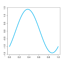
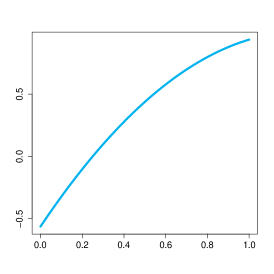
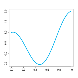
Figure 1: Functional slopes corresponding to the three FLMSR considered in the simulations. Left: $\beta_{1}$. Middle: $\beta_{2}$. Right: $\beta_{3}$.

	$\delta_{0}=0.00$	$\delta_{1}=0.01$	$\delta_{2}=0.02$	$\delta_{3}=0.03$
$\beta_{1}$	$0.8232$	$0.8244$	$0.8285$	$0.8334$
$\beta_{2}$	$0.9490$	$0.9491$	$0.9495$	$0.9500$
$\beta_{3}$	$0.9709$	$0.9710$	$0.9712$	$0.9713$

Table 1: Coefficients of determination

Firstly, Figure 2 shows the logarithm of the estimated MSEEs of the eight estimators of $\beta$ for the three FLMSRs and the three values of $\gamma$ considered for $n=100$. Three comments are in order. First, as expected, the estimators obtained with all the observed responses, denoted by $\widehat{\beta}_{\mathcal{C}}$ and $\widehat{\beta}_{\mathcal{CL}}$, respectively, have lower MSEE than estimators obtained with missing responses. However, the differences between the MSEEs of $\widehat{\beta}_{\mathcal{C}}$ and $\widehat{\beta}_{\mathcal{CL}}$ with respect to the imputed estimators $\widehat{\beta}_{\mathcal{I}}$ and $\widehat{\beta}_{\mathcal{IL}}$ are very small, especially when $\gamma$ increases and, therefore, the number of missing responses decreases. Second, as also expected the imputed estimators $\widehat{\beta}_{\mathcal{I}}$, $\widehat{\beta}_{\mathcal{IL}}$, $\widehat{\beta}_{\mathcal{W}}$, and $\widehat{\beta}_{\mathcal{WL}}$ have lower estimated MSSEs than the simplified estimators $\widehat{\beta}_{\mathcal{S}}$ and $\widehat{\beta}_{\mathcal{SL}}$, especially for the first and third FLMSRs. For the second FLMSR the differences are much smaller, possibly because $\beta_{2}$ is the simplest of the three considered. Third, there is no consensus as to whether or not OLS and CV-based estimators are better than LASSO-based estimators. For the first FLMSR, the former estimators are better, but for the second, the latter are slightly better. The conclusions for $n=50$ and $n=200$ are similar, except that the larger the sample size, the smaller the MSEEs.

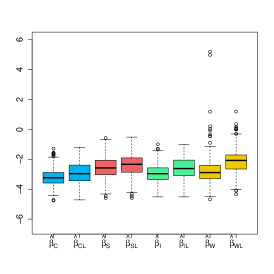
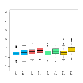
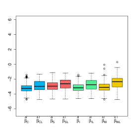
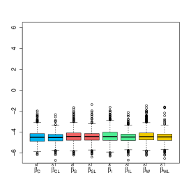
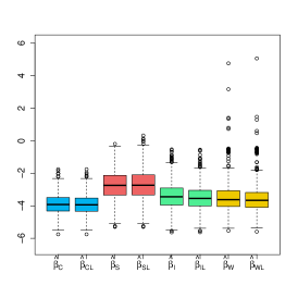
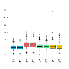
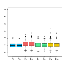
Figure 2: Logarithms of MSEEs for the eight estimators of $\beta_{1},\beta_{2},\beta_{3}$ (columns, from left to right) and $\gamma=0.5,1,2$ (rows, from top to down) for $n=100$.

Secondly, Figure 3 shows the logarithm of the time (in seconds) needed to compute such estimators for the eight estimators of $\beta$ for the three sample sizes considered for the first FLMSR and $\gamma=1$. Three comments are in order. First, as might be expected, simplified estimators are the fastest to compute, since they only use the pairs with observed responses. However, as we have seen above, imputed estimators perform better than simplified estimators at the cost of slightly increasing the computational cost. Second, estimators based on OLS and CV are computationally less demanding than LASSO-selected estimators, without reducing their estimated MSEEs. Third, the inverse probability weighted estimators $\widehat{\beta}_{\mathcal{W}}$ and $\widehat{\beta}_{\mathcal{WL}}$ are the most computationally expensive, which is expected given that these estimators require computing the Nadaraya–Watson estimator of the MAR mechanism $p\left(\cdot\right)$ in (12). The conclusions for $n=50$ and $n=200$ and for $\gamma=0.5$ and $\gamma=2$ are similar; only the computation cost in each case varies similarly to the cases shown.

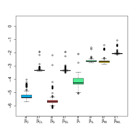
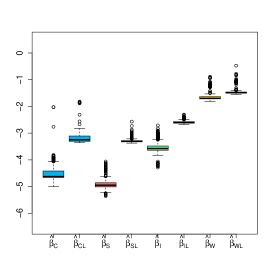
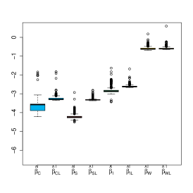
Figure 3: Logarithms of times (in seconds) needed to compute the eight estimators of $\beta$ for the three sample sizes considered for $\beta_{1}$ and $\gamma=1$.

Table 2: Rejection frequencies of the null hypothesis for significance level $\alpha=0.05$ for FLMSR 1.

		$\gamma=0.5$
$n$	$\delta$	$\widehat{\beta}_{\mathcal{C}}$	$\widehat{\beta}_{\mathcal{CL}}$	$\widehat{\beta}_{\mathcal{S}}$	$\widehat{\beta}_{\mathcal{SL}}$	$\widehat{\beta}_{\mathcal{I}}$	$\widehat{\beta}_{\mathcal{IL}}$	$\widehat{\beta}_{\mathcal{W}}$	$\widehat{\beta}_{\mathcal{WL}}$
50	0.00	0.065	0.064	0.053	0.054	0.059	0.058	0.046	0.035
	0.01	0.161	0.163	0.142	0.148	0.156	0.159	0.145	0.137
	0.02	0.412	0.401	0.316	0.306	0.369	0.348	0.343	0.292
	0.03	0.666	0.651	0.540	0.512	0.598	0.556	0.549	0.475
100	0.00	0.055	0.055	0.056	0.051	0.060	0.054	0.059	0.051
	0.01	0.254	0.255	0.224	0.219	0.247	0.239	0.249	0.228
	0.02	0.727	0.715	0.640	0.629	0.666	0.650	0.685	0.647
	0.03	0.951	0.944	0.900	0.900	0.916	0.913	0.909	0.879
200	0.00	0.056	0.055	0.053	0.055	0.056	0.056	0.054	0.052
	0.01	0.462	0.461	0.458	0.453	0.475	0.469	0.479	0.479
	0.02	0.964	0.963	0.937	0.931	0.947	0.937	0.951	0.932
	0.03	0.999	0.999	0.999	0.998	0.998	0.997	0.994	0.994
		$\gamma=1$
50	0.00	0.072	0.069	0.059	0.055	0.067	0.061	0.064	0.060
	0.01	0.150	0.148	0.143	0.147	0.167	0.162	0.163	0.137
	0.02	0.394	0.380	0.372	0.359	0.402	0.378	0.398	0.351
	0.03	0.671	0.645	0.618	0.599	0.670	0.632	0.666	0.585
100	0.00	0.057	0.055	0.055	0.053	0.058	0.057	0.058	0.058
	0.01	0.259	0.254	0.254	0.251	0.266	0.260	0.279	0.265
	0.02	0.719	0.707	0.731	0.720	0.746	0.726	0.751	0.730
	0.03	0.947	0.946	0.934	0.932	0.943	0.942	0.944	0.939
200	0.00	0.056	0.058	0.057	0.060	0.063	0.066	0.065	0.066
	0.01	0.479	0.477	0.509	0.495	0.518	0.511	0.525	0.506
	0.02	0.968	0.966	0.970	0.967	0.977	0.974	0.978	0.971
	0.03	1.000	1.000	1.000	1.000	1.000	1.000	1.000	0.999
		$\gamma=2$
50	0.00	0.046	0.044	0.055	0.059	0.055	0.060	0.056	0.057
	0.01	0.142	0.136	0.156	0.155	0.176	0.169	0.175	0.166
	0.02	0.385	0.378	0.402	0.392	0.419	0.405	0.419	0.385
	0.03	0.674	0.655	0.676	0.659	0.695	0.672	0.697	0.652
100	0.00	0.063	0.057	0.057	0.056	0.055	0.053	0.057	0.053
	0.01	0.255	0.248	0.270	0.270	0.286	0.279	0.291	0.278
	0.02	0.741	0.712	0.758	0.749	0.777	0.754	0.783	0.753
	0.03	0.952	0.946	0.957	0.952	0.959	0.954	0.959	0.957
200	0.00	0.052	0.052	0.049	0.049	0.057	0.056	0.054	0.053
	0.01	0.512	0.508	0.558	0.556	0.559	0.559	0.568	0.551
	0.02	0.963	0.965	0.980	0.977	0.983	0.979	0.984	0.976
	0.03	1.000	1.000	1.000	1.000	1.000	1.000	1.000	1.000

		$\gamma=0.5$
$n$	$\delta$	$\widehat{\beta}_{\mathcal{C}}$	$\widehat{\beta}_{\mathcal{CL}}$	$\widehat{\beta}_{\mathcal{S}}$	$\widehat{\beta}_{\mathcal{SL}}$	$\widehat{\beta}_{\mathcal{I}}$	$\widehat{\beta}_{\mathcal{IL}}$	$\widehat{\beta}_{\mathcal{W}}$	$\widehat{\beta}_{\mathcal{WL}}$
50	0.00	0.051	0.051	0.047	0.049	0.052	0.051	0.050	0.037
	0.01	0.171	0.170	0.124	0.119	0.151	0.146	0.137	0.126
	0.02	0.386	0.388	0.303	0.300	0.349	0.341	0.314	0.278
	0.03	0.692	0.688	0.543	0.545	0.596	0.591	0.552	0.504
100	0.00	0.040	0.040	0.043	0.043	0.049	0.049	0.057	0.047
	0.01	0.269	0.256	0.219	0.215	0.230	0.237	0.242	0.231
	0.02	0.689	0.688	0.618	0.620	0.663	0.667	0.682	0.662
	0.03	0.961	0.965	0.899	0.900	0.927	0.925	0.925	0.904
200	0.00	0.044	0.044	0.053	0.053	0.051	0.054	0.056	0.053
	0.01	0.446	0.438	0.444	0.443	0.463	0.461	0.463	0.464
	0.02	0.947	0.947	0.937	0.937	0.949	0.947	0.948	0.940
	0.03	1.000	1.000	0.999	0.998	1.000	0.999	0.998	0.997
		$\gamma=1$
50	0.00	0.059	0.059	0.052	0.054	0.059	0.059	0.052	0.059
	0.01	0.155	0.152	0.142	0.143	0.151	0.153	0.150	0.145
	0.02	0.415	0.412	0.393	0.397	0.435	0.439	0.421	0.393
	0.03	0.690	0.684	0.649	0.640	0.673	0.675	0.674	0.641
100	0.00	0.061	0.060	0.053	0.053	0.057	0.055	0.053	0.052
	0.01	0.247	0.248	0.252	0.250	0.262	0.266	0.276	0.268
	0.02	0.699	0.706	0.715	0.718	0.730	0.741	0.744	0.738
	0.03	0.956	0.957	0.957	0.956	0.959	0.964	0.961	0.959
200	0.00	0.038	0.044	0.050	0.049	0.049	0.051	0.051	0.052
	0.01	0.489	0.486	0.483	0.481	0.495	0.494	0.496	0.499
	0.02	0.963	0.960	0.967	0.966	0.972	0.968	0.973	0.970
	0.03	1.000	1.000	1.000	1.000	1.000	1.000	1.000	1.000
		$\gamma=2$
50	0.00	0.058	0.056	0.056	0.057	0.059	0.054	0.052	0.051
	0.01	0.145	0.140	0.141	0.141	0.145	0.144	0.149	0.139
	0.02	0.440	0.445	0.475	0.480	0.484	0.487	0.483	0.479
	0.03	0.698	0.694	0.716	0.714	0.730	0.719	0.739	0.718
100	0.00	0.054	0.056	0.041	0.040	0.042	0.040	0.041	0.039
	0.01	0.276	0.272	0.297	0.298	0.306	0.300	0.308	0.304
	0.02	0.746	0.748	0.768	0.768	0.774	0.774	0.780	0.775
	0.03	0.948	0.949	0.956	0.958	0.958	0.959	0.960	0.959
200	0.00	0.047	0.045	0.054	0.059	0.053	0.060	0.052	0.060
	0.01	0.449	0.439	0.512	0.519	0.524	0.519	0.520	0.520
	0.02	0.952	0.949	0.966	0.969	0.970	0.971	0.973	0.974
	0.03	1.000	0.999	1.000	1.000	1.000	1.000	1.000	1.000

Table 3: Rejection frequencies of the null hypothesis for significance level $\alpha=0.05$ for FLMSR 2.

		$\gamma=0.5$
$n$	$\delta$	$\widehat{\beta}_{\mathcal{C}}$	$\widehat{\beta}_{\mathcal{CL}}$	$\widehat{\beta}_{\mathcal{S}}$	$\widehat{\beta}_{\mathcal{SL}}$	$\widehat{\beta}_{\mathcal{I}}$	$\widehat{\beta}_{\mathcal{IL}}$	$\widehat{\beta}_{\mathcal{W}}$	$\widehat{\beta}_{\mathcal{WL}}$
50	0.00	0.064	0.068	0.039	0.032	0.047	0.047	0.054	0.051
	0.01	0.152	0.153	0.095	0.088	0.136	0.126	0.126	0.104
	0.02	0.416	0.419	0.252	0.246	0.361	0.348	0.330	0.298
	0.03	0.675	0.668	0.461	0.434	0.583	0.543	0.532	0.467
100	0.00	0.048	0.048	0.042	0.041	0.052	0.055	0.059	0.053
	0.01	0.265	0.262	0.176	0.171	0.243	0.239	0.256	0.240
	0.02	0.739	0.738	0.577	0.577	0.667	0.674	0.678	0.650
	0.03	0.949	0.949	0.853	0.857	0.918	0.921	0.924	0.900
200	0.00	0.045	0.046	0.036	0.035	0.051	0.045	0.052	0.047
	0.01	0.485	0.488	0.391	0.390	0.448	0.447	0.464	0.463
	0.02	0.950	0.946	0.904	0.904	0.937	0.940	0.947	0.944
	0.03	1.000	1.000	0.994	0.995	0.999	0.999	0.993	0.989
		$\gamma=1$
50	0.00	0.061	0.063	0.045	0.044	0.060	0.065	0.067	0.062
	0.01	0.147	0.148	0.122	0.120	0.149	0.145	0.151	0.145
	0.02	0.411	0.410	0.335	0.342	0.416	0.414	0.419	0.397
	0.03	0.686	0.676	0.572	0.569	0.694	0.663	0.678	0.614
100	0.00	0.057	0.056	0.046	0.045	0.059	0.057	0.055	0.058
	0.01	0.260	0.259	0.261	0.257	0.278	0.283	0.293	0.291
	0.02	0.738	0.744	0.672	0.668	0.722	0.721	0.739	0.727
	0.03	0.958	0.954	0.922	0.924	0.951	0.950	0.952	0.948
200	0.00	0.046	0.059	0.042	0042	0.039	0.040	0.043	0.041
	0.01	0.462	0.455	0.459	0.458	0.501	0.498	0.495	0.497
	0.02	0.961	0.960	0.956	0.955	0.968	0.966	0.969	0.963
	0.03	1.000	1.000	1.000	1.000	1.000	1.000	1.000	1.000
		$\gamma=2$
50	0.00	0.058	0.060	0.056	0.053	0.064	0.064	0.060	0.061
	0.01	0.158	0.159	0.147	0.144	0.177	0.173	0.181	0.176
	0.02	0.406	0.400	0.378	0.380	0.432	0.426	0.440	0.421
	0.03	0.692	0.682	0.666	0.662	0.715	0.699	0.721	0.690
100	0.00	0.051	0.049	0.042	0.041	0.049	0.050	0.047	0.048
	0.01	0.275	0.271	0.261	0.259	0.277	0.278	0.274	0.270
	0.02	0.727	0.728	0.738	0.735	0.762	0.760	0.763	0.760
	0.03	0.942	0.945	0.945	0.949	0.954	0.955	0.959	0.957
200	0.00	0.049	0.050	0.063	0.062	0.062	0.062	0.064	0.062
	0.01	0.458	0.455	0.505	0.507	0.518	0.516	0.521	0.519
	0.02	0.962	0.961	0.967	0.968	0.970	0.971	0.972	0.972
	0.03	1.000	1.000	1.000	1.000	1.000	1.000	1.000	1.000

Table 4: Rejection frequencies of the null hypothesis for significance level $\alpha=0.05$ for FLMSR 3.

To analyze the performance of the proposed testing procedures under the composite hypothesis (2), we consider a model of the form:

$$Y=\left\langle\mathcal{X},\beta_{j}\right\rangle+\delta_{k}\left\|\mathcal{X}\right\|_{\mathbb{H}}^{2}+\varepsilon,$$

where the functional predictor $\mathcal{X}$, the functional slopes $\beta_{j}$, for $j=1,2,3$, and the error variance $\sigma^{2}$ take the same values as in the first simulation experiment, while $\delta_{k}=0.01\cdot k$, for $k=0,1,2,3$, is a coefficient that measures the degree of deviation from the null hypothesis. Obviously, $\delta_{0}=0$ implies that we are under the null hypothesis (2), which allows us to analyze the behavior of the test procedure under that hypothesis, while the remaining values imply that we are under the alternative hypothesis such that the higher $\delta_{k}$ is, the further we are from $H_{0}$, which allows us to analyze the behavior of the test procedures under that hypothesis. The resulting coefficients of determination are those that appear in Table 1 for each model and value of $\delta_{k}$. Note how little effect the nonlinear part of the FLMSRs has even for high values of $\delta_{k}$. This implies that detecting such nonlinearity can be challenging. Besides, the observance probability, the parameters $\gamma$, the sample sizes $n$ and the number of data sets generated for each FLMSR are exactly the same as in the previous simulation experiment. Additionally, to compute the $p$-values we use $B=1000$ bootstrap samples. We then proceed as in the previous experiment by generating a data set with all observed responses and subsequently generating missing responses with the corresponding observance probability and associated parameter $\gamma$. Then, for each generated data set with observed responses, we run the testing procedure in García-Portugués et al., (2014) for the FPC estimator of $\beta$ in Cardot et al., (2007) and the LASSO-selected estimator in García-Portugués et al., (2020), while for each generated data set with missing responses, we run the testing procedure for the six estimators of $\beta$ in Section 3 and the associated residuals (19). Tables 2, 3, and 4 show the rejection frequencies of the null hypothesis for the significance level $\alpha=0.05$ for the three FLMSRs considered, the eight estimates of $\beta$, the three values of the parameter $\gamma$, the three sample sizes, and the four coefficients $\delta_{k}$.

Several comments are in order in view of these three tables. First, the procedure seems to be able to calibrate well the size of the tests, in this case $\alpha=0.05$, since there do not seem to be large deviations with respect to this value. The largest deviation is found in the first FLMSR, with $\gamma=1$ and $n=50$, where the rejection frequency of the null hypothesis is $0.073$. Second, considering the small effect of the nonlinear part of the model even for $\delta_{3}$, the procedure, with and without missing responses, seems to be able to detect such nonlinearity in a large number of generated data sets, which indicates that the performance of the procedure is very satisfactory. Third, in the vast majority of cases, the frequency of rejection of the null hypothesis under the alternative is higher for estimators obtained with the full sample. It is true that for the first FLMSR there are cases where paradoxically this is not the case, but this is most likely due to small size distortions. Fourth, although the differences may sometimes seem small, there is a pattern that indicates that the imputed and inverse probability weighted estimators are more powerful than the simplified imputed estimators. Of course, the larger the sample size, the smaller the difference between the estimators. However, we can find larger differences when the sample size is not large. For example, for the third FLMSR, in the case $n=50$, $\gamma=0.5$, and $\delta=0.2$, the relative increase in rejection frequency between the imputed and the simplified estimator is $43.25\%$, while in the case $n=100$, $\gamma=0.5$, and $\delta=0.1$, the relative increase in rejection frequency between the inverse probability weighted and the simplified estimator is $45.45\%$. Fifth, as expected, the smaller the values of $\gamma$ and/or $n$, the lower the frequency of rejection of estimators based on samples with missing responses. Sixth, there do not appear to be major differences between the OLS- and CV-based estimators and the LASSO-based estimators, so either can be used to test linearity. Quite possibly, the main conclusion is that there is a loss in the power of the test if missing responses are simply discarded, especially when the sample size is not large.

6 Real data example

To exemplify the use in practice of the proposed procedure, we use a real data set previously analyzed in Febrero-Bande et al., (2019). In this data set, the functional predictor is the mean curve of the annual average daily temperature observed in $73$ Spanish weather stations for the period $1980$–$2009$, and the real response is the average of the total number of sunny days per year, where a sunny day means that there are no opaque clouds during more than $80\%$ of daylight hours. The top left panel of Figure 4 shows the temperatures corresponding to the $73$ weather stations after a B-spline smoothing. As it can be seen, there is a small group of temperatures that are clustered together and that have a different shape from the majority of curves. These temperatures correspond to stations in the Canary Islands and are not considered in the analysis. Moreover, there is a curve with very low temperatures that corresponds to a station located in the Port of Navacerrada, one of the coldest places in Spain. Due to its outlying behavior, this curve is also not considered in the analysis. The mean curves of the annual average daily temperature per year of the remaining $65$ stations are shown in the bottom left panel of Figure 4. In the figure, the temperatures corresponding to missing responses are shown in red and, as it can be seen, these temperatures appear mainly in the center, suggesting that the MAR hypothesis is reasonable here as the missing responses correspond to weather stations with mild temperatures. The figure also shows boxplots of the $50$ observed responses with and without the temperatures removed. The percentage of missing responses is $20.63\%$.

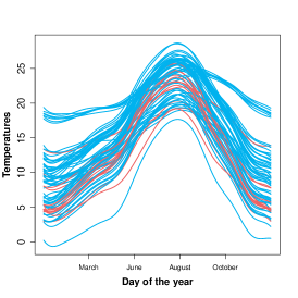
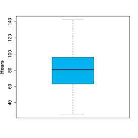
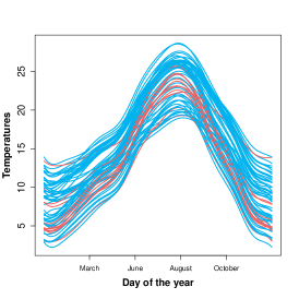
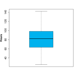
Figure 4: Left: Average daily temperatures. Right: Average number of sunny days per year. Top: Data with all the observations. Bottom: Data without a set of stations in the Canary Islands and Navacerrada.

As mentioned in the introduction, Febrero-Bande et al., (2019) used an FLMSR to predict the average number of sunny days per year with the annual average daily temperatures. Here, the main goal is to check such linearity assumption taking into account the existence of missing responses. For this purpose, we carry out the testing procedure for the six estimators of the functional slope of the FLMSR considered. As in the simulations, we consider $B=1000$ bootstrap samples for the computation of the $p$-values associated with the hypothesis test with each of the $\beta$ estimators. The first three FPCs of the average daily temperatures explain the $99.63\%$ of the total variability of the temperatures, the last of them explaining only the $0.55\%$ of the total. Therefore, we fix $K_{\max}=3$ since taking a larger number may result in a large increase in the mean squared error of estimation of $\beta$. After that, we perform the estimation of $\beta$ with the six methods considered together with the computation of the associated residuals, necessary to obtain the corresponding statistics. The six estimators are shown in Figure 5. Note the clear difference between the OLS+CV estimators and the LASSO estimators, which is due to the fact that the former select $3$ FPCs and the latter $2$ FPCs. Since fewer FPCs are used, the variability of the LASSO estimators is lower. Furthermore, it can be seen that the simplified OLS+CV estimator is somewhat different from the other two OLS+CV estimators so the impact of the imputations seems to be relevant. Finally, Figure 6 shows the test statistics, the bootstrap statistics, and a kernel density estimate of the latter. In particular, the $p$-values are $0.386$, $0.187$, $0.345$, $0.223$, $0.464$, and $0.253$, respectively for such estimators, which indicate that the procedure does not reject the linearity hypothesis with any of the six estimators considered. Consequently, a linear model such as the one used in Febrero-Bande et al., (2019)seems adequate to explain the average of the total number of sunny days per year with the mean curve of the annual average daily temperature when there are missing responses when the first variable is not completely observed. In particular, note the difference in $p$-values depending on whether the estimator is OLS+CV or LASSO. In any case, the test results are similar even if the FLMSR functional slope estimate is different. [2]

Figure 5: Estimators of the functional slope of the FLMSR.

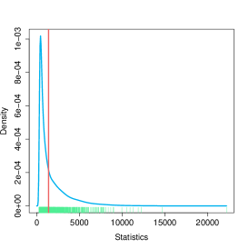
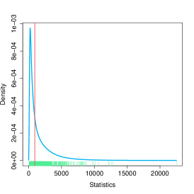
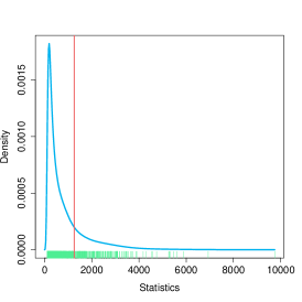
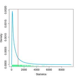
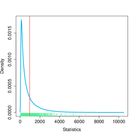
Figure 6: From left to right and from top to bottom, the panels show the test statistics (vertical lines) and the kernel density estimators of the bootstrapped statistics for the tests run with $\widehat{\beta}_{\mathcal{S}}$, $\widehat{\beta}_{\mathcal{I}}$, $\widehat{\beta}_{\mathcal{W}}$, $\widehat{\beta}_{\mathcal{SL}}$, $\widehat{\beta}_{\mathcal{IL}}$, and $\widehat{\beta}_{\mathcal{WL}}$, respectively. The respective $p$-values are $0.386$, $0.345$, $0.464$, $0.187$, $0.223$, and $0.253$.

7 Conclusions

We have proposed a goodness-of-fit testing procedure for the null hypothesis of the functional linear model with scalar response when some of the responses are missing at random. More precisely, the procedure is an adaptation to the case of MAR responses of the procedure proposed by García-Portugués et al., (2014). Six different estimation methods for the functional slope of the model were considered, although the ones that seem to show the best performance in terms of testing are the imputed and inverse probability weighted estimators. Note that this implies that testing with only pairs of observations with observed responses is not the best option. The simulation analysis shows that the procedure behaves well in practice because it respects the significant level and has sufficient power to detect non-linearities even when their effect is small. The procedure was used with a real data set to determine if the FLMSR is a valid model for the data, and no evidence was found to reject the linearity hypothesis.

Although in this article we focused on the FLMSR, the proposed testing procedure can be extended to checking for any other regression model with functional covariate and scalar response. Indeed, as the test statistic is based on residuals, the practical implementation and the wild bootstrap calibration would not differ if similar models are considered in which an estimation mechanism appropriate to the case of the existence of MAR responses would be required. Of course, an obvious extension is the use of several functional covariates or any alternative functional expression to the linear one.

References

- Bianco et al., (2019) Bianco, A., Boente, G., González-Manteiga, W., and Pérez-González, A. (2019). Plug-in marginal estimation under a general regression model with missing responses and covariates. Test, 28(1):106–146.
- Bianco et al., (2020) Bianco, A., Boente, G., González-Manteiga, W., and Pérez-González, A. (2020). Robust location estimators in regression models with covariates and responses missing at random. J. Nonparametr. Stat., 32(4):915–939.
- Cardot et al., (2007) Cardot, H., Mas, A., and Sarda, P. (2007). CLT in functional linear regression models. Probab. Theory Related Fields, 138(3-4):325–361.
- Ciarleglio et al., (2022) Ciarleglio, A., Petkova, E., and Harel, O. (2022). Elucidating age and sex-dependent association between frontal EEG asymmetry and depression: An application of multiple imputation in functional regression. J. Am. Stat. Assoc., 117(537):12–26.
- Crambes and Henchiri, (2019) Crambes, C. and Henchiri, Y. (2019). Regression imputation in the functional linear model with missing values in the response. J. Stat. Plan. Inference, 201:103–119.
- Cuesta-Albertos et al., (2019) Cuesta-Albertos, J. A., García-Portugués, E., Febrero-Bande, M., and González-Manteiga, W. (2019). Goodness-of-fit tests for the functional linear model based on randomly projected empirical processes. Ann. Stat., 47(1):439–467.
- Febrero-Bande et al., (2017) Febrero-Bande, M., Galeano, P., and González-Manteiga, W. (2017). Functional principal component regression and functional partial least-squares regression: an overview and a comparative study. Int. Stat. Rev., 85(1):61–83.
- Febrero-Bande et al., (2019) Febrero-Bande, M., Galeano, P., and González-Manteiga, W. (2019). Estimation and prediction for the functional linear model with scalar response with responses missing at random. Comput. Stat. Data Anal., 131:91–103.
- Ferraty et al., (2013) Ferraty, F., Sued, M., and Vieu, P. (2013). Mean estimation with data missing at random for functional covariables. Statistics, 47(4):688–706.
- Ferraty and Vieu, (2006) Ferraty, F. and Vieu, P. (2006). Nonparametric Functional Data Analysis: Theory and Practice. Springer Series in Statistics. Springer, New York.
- Friedman et al., (2010) Friedman, J., Hastie, T., and Tibshirani, R. (2010). Regularization paths for generalized linear models via coordinate descent. J. Stat. Softw., 33(1):1–22.
- García-Portugués et al., (2020) García-Portugués, E., Álvarez-Liébana, J., Álvarez-Pérez, G., and González-Manteiga, W. (2020). A goodness-of-fit test for the functional linear model with functional response. Scand. J. Stat., 48(2):502–528.
- García-Portugués et al., (2014) García-Portugués, E., González-Manteiga, W., and Febrero-Bande, M. (2014). A goodness-of-fit test for the functional linear model with scalar response. J. Comput. Graph. Stat., 23(3):761–778.
- González-Manteiga, (2023) González-Manteiga, W. (2023). A review on specification tests for models with functional data. Span. J. Stat., 4(1):9–40.
- González-Manteiga et al., (2023) González-Manteiga, W., Crujeiras, R. M., and García-Portugués, E. (2023). A review of goodness-of-fit tests for models involving functional data. In Balakrishnan, N., Gil, M. A., Martín, N., Morales, D., and Pardo, M. C., editors, Trends in Mathematical, Information and Data Sciences, volume 445 of Studies in Systems, Decision and Control, pages 349–358. Springer, Cham.
- González-Manteiga and Pérez-González, (2006) González-Manteiga, W. and Pérez-González, A. (2006). Goodness-of-fit tests for linear regression models with missing response data. Can. J. Stat., 34(1):149–170.
- Greven and Scheipl, (2017) Greven, S. and Scheipl, F. (2017). A general framework for functional regression modelling. Stat. Model., 17(1-2):1–35.
- Horváth and Kokoszka, (2012) Horváth, L. and Kokoszka, P. (2012). Inference for Functional Data with Applications. Springer Series in Statistics. Springer, New York.
- Hsing and Eubank, (2015) Hsing, T. and Eubank, R. (2015). Theoretical Foundations of Functional Data Analysis, with an Introduction to Linear Operators. Wiley Series in Probability and Statistics. John Wiley & Sons, Chichester.
- Kokoszka and Reimherr, (2017) Kokoszka, P. and Reimherr, M. (2017). Introduction to Functional Data Analysis. Texts in Statistical Science Series. CRC Press, Boca Raton.
- Li, (2012) Li, X. (2012). Lack-of-fit testing of a regression model with response missing at random. J. Stat. Plan. Inference, 142(12):155–170.
- Ling et al., (2022) Ling, N., Cheng, L., Vieu, P., and Ding, H. (2022). Missing responses at random in functional single index model for time series data. Stat. Pap., 63(2):665–692.
- Ling et al., (2015) Ling, N., Liang, L., and Vieu, P. (2015). Nonparametric regression estimation for functional stationary ergodic data with missing at random. J. Stat. Plan. Inference, 162:75–87.
- Ling et al., (2016) Ling, N., Liu, Y., and Vieu, P. (2016). Conditional mode estimation for functional stationary ergodic data with responses missing at random. Statistics, 50(5):991–1013.
- Mammen, (1993) Mammen, E. (1993). Bootstrap and wild bootstrap for high dimensional linear models. Ann. Stat., 21(1):255–285.
- McLean et al., (2015) McLean, M. W., Hooker, G., and Ruppert, D. (2015). Restricted likelihood ratio tests for linearity in scalar-on-function regression. Stat. Comput., 25(5):997–1008.
- Pérez González et al., (2021) Pérez González, A., Cotos-Yáñez, T. R., González-Manteiga, W., and Crujeiras, R. M. (2021). Goodness-of-fit tests for quantile regression with missing responses. Stat. Pap., 62(3):1231–1264.
- Qin et al., (2017) Qin, J., Zhang, B., and Leung, D. H. Y. (2017). Efficient augmented inverse probability weighted estimation in missing data problems. J. Bus. Econ. Stat., 35(1):86–97.
- Ramsay and Silverman, (2005) Ramsay, J. O. and Silverman, B. W. (2005). Functional Data Analysis. Springer Series in Statistics. Springer, New York.
- Reiss et al., (2017) Reiss, P. T., Goldsmith, J., Shang, H. L., and Ogden, R. T. (2017). Methods for scalar-on-function regression. Int. Stat. Rev., 85(2):228–249.
- Sun et al., (2017) Sun, Z., Chen, F., Zhou, X., and Zhang, Q. (2017). Improved model checking methods for parametric models with responses missing at random. J. Multivar. Anal., 154:147–161.
- Sun and Wang, (2009) Sun, Z. and Wang, Q. (2009). Checking the adequacy of a general linear model with responses missing at random. J. Stat. Plan. Inference, 139(10):3588–3604.
- Zheng et al., (2020) Zheng, S.-J., Gao, S.-Y., and Sun, Z.-H. (2020). Projection-based consistent test for linear regression model with missing response and covariates. Acta. Math. Appl. Sin., 36(4):917–935.