Weight Try-Once-Discard Protocol-Based $L_{2}$-$L_{\infty}$ State Estimation for Markovian Jumping Neural Networks with Partially Known Transition Probabilities

Abstract

1 Introduction

For nearly decades, it is generally known that artificial neural networks (ANNs) have been continuously promoted and improved in different fields including signal transmission, memory storage and image recognition. However, in practical engineering applications, actuator failure, parameter drift and changes in internal connections of subsystems often occur in actual control network systems, and these negative situations will randomly affect the structure of the control system. Therefore, the Markovian jumping neural networks (MJNNs) have been put forward and widely applied by more and more experts because of its effective modeling capability, which is a random switching system with multiple modes. Considerable related research conclusions have been shown in Li-Zuo-Wang ; Daafouz-Riedinger-Iung ; Hua-Zheng-Deng ; Liang-Dai-Shen-Wang and the references therein.

As is well known, transition probability determines the operation of the whole MJNNs. In an ideal situation, the analysis and design of the system are simple and convenient. Therefore, a large number of existing studies on MJNNs are obtained when the transition probability is fully known. In practical, when the system is modeled as MJNNs, it is difficult to fully know the transition probability of the system jumping between modes according to great difficulty and high cost. Therefore, instead of spending a lot of manpower and material resources to obtain the complete transition probability, from the control point of view, it is better to further study the more general MJNNs whose transition probability is partially unknown. In recent years, many studies based on it have been pay attention, see Yao-Liu-Lu-Xu-Zhou ; Shen-13 ; Cui-Sun-Fang-Xu-Zhao ; Yin-Shi-Liu-Liu ; Zhang-B-L ; Wang-1 .

In engineering applications, it is very critical to get the real state of the system for practical applications such as image recognition. It deserves to note that, the ability to obtain total state information is not enough due to physical limitations and technical difficulties. Consequently, state estimation method has been more and more recognized and studied in engineering control, which gives important rein to obtain real neuron state. As for state estimation problem for MJNNs has recently become a hot topic of research with a great number of results reported in the literature, see Ji-Zhang-T ; Liu-Shen-Li ; Wang-Wang-Liu10 ; Zhao-Wang-Zou-Liu ; Liu-Wang-Fei-Dong and the reference therein. For instance,

On the other side, in the zone of state estimation, it is often the case that the system performance should be considered to deal with the exogenous disturbances. For unknown but energy bounded disturbances, one can resort to the $H_{\infty}$ and $L_{2}$-$L_{\infty}$ performance indexes. Regarding that the $L_{2}$-$L_{\infty}$ state estimation is able to constrain the effect from the energy-bounded external disturbances with unknown statistical characteristic on the estimation error. On ground of the above analysis, plenty of research results have been obtained in the analysis of $L_{2}$-$L_{\infty}$ state estimation issue for MJNNs, see Chen-Zheng ; Shen-Wang-Shen ; Qian-Chen-Liu-Fe ; Qian-Li-Chen-Yang ; Qian-Li-Zhao-Chen ; Shen-Xing-Wu-Cao-Huang . However, in this paper the estimation problem for partially unknown transition probabilities in MJNNs are rarely mentioned and studied.

On another research hotspot is communication protocols, which can orchestrate the transmission order of sensor nodes. In major existing literatures about the estimation issue of MJNNs, there is an assumption that sensor nodes can receive transmission signals from the network at the same time. Nonetheless, it is usually impractical for networked systems because practical networks inevitably are subject to limited bandwidth which lead to data conflicts when encountering multiple information accesses. In contrast with those traditional approaches without protocol scheduling, the introduction of communication protocol would cause some fundamental challenges to dynamic analysis. Up to now, there have been some elementary results about the MJNNs constrained by communication protocols including Round-Robin protocol (RRP), stochastic communication protocol (SCP) and weight try-once-discard protocol (WTOD protocol), see Li-Wang-Dong-Fei ; Zou-Wang-Han-Zhou ; Long-P-Ye ; Liu-Wang-Ma-Zhang-Bo ; Zou-Wang-Gao ; Zhang-Peng ; Shen-Wang-Shen-F ; Ju-Wei-Ding-Liu ; Aslam-Dai ; Chen-Hu-Yu-Chen-Du . As such, the WTOD protocol is a kind of quadratic protocols, which differs from the periodic allocation of RRP. It can dispatch the transmission instants to certain sensor nodes based on a given quadratic selection principle. For instance, in Aslam-Dai . Therefore, it is more challenging to develop the communication protocol approach to address the Chen-Hu-Yu-Chen-Du $L_{2}$-$L_{\infty}$ state estimation problem for delayed MJNNs with partially known transition probabilities.

In view of the above-mentioned discussion, our intention is on the $L_{2}$-$L_{\infty}$ state estimation issue for a class of delayed MJNNs with partially known transition probabilities based on the WTOD protocol. The elementary contributions of this paper are outlined as follows:

1

It was the $L_{2}$-$L_{\infty}$ performance index that for the first time is initiated into the discussion on state estimation of delayed MJNNs with with partially known transition probabilities, which provides a more general promotion for the estimation error.

2

The WTOD protocol is adopted to dispatch the sensor nodes so as to effectively alleviate the updating frequency of output signals.

3

The hybrid effects of the time delays, Markov chain, and protocol parameters are apparently reflected in the co-designed estimator which can be solved by a combination of comprehensive matrix inequalities.

$\mathbf{Notations}.$ The notation used in this paper is normative. There are the $n$-dimensional Euclidean space $\mathbb{R}^{n}$ and the sets of positive integers $\mathbb{Z}^{+}$; $\|\cdot\|$ means the Euclidean norm; $I$, $0$ represent the identity matrix, and zero matrix with appropriate dimensions, respectively. Let $\mathbb{E}\{\cdot\}$ is expressed as the mathematical expectation. $P>0$ stands for that $P$ is a real symmetric positive definite matrix. $\text{diag}\{\cdots\}$ denotes a block diagonal matrix. We use the notation $*$ as the ellipsis of symmetry terms. $\otimes$ represents the Kronecker product.

2 Model Prescription and Lemmas

2.1 MJNNs Establishment

We consider the discrete-time MJNNs with time-varying delays and energy-bounded exogenous disturbances described as follows:

$$\left\{\begin{array}[]{cll}x(k+1)&=A(r_{k})x(k)+B(r_{k})f(x(k))+C(r_{k})f(x(k-\tau(k))+D_{1}(r_{k})\omega(k)\\ y(k)&=E(r_{k})x(k)+D_{2}(r_{k})v(k)\\ z(k)&=M(r_{k})x(k)\\ \end{array}\right.$$ (4)

where $x(k)=[x_{1}(k)\ \ \cdots\ \ x_{n}(k)]^{T}\in\mathbb{R}^{n}$ is the neuron state vector, $y(k)=[y_{1}(k)\ \ \cdots\ \ y_{m}(k)]^{T}\in\mathbb{R}^{m}$ is the measurement output of NNs, and $z(k)\in\mathbb{R}^{q}$ is the output vector to be estimated. $f(x(k)):\mathbb{R}^{n}\longrightarrow\mathbb{R}^{n}$ is nonlinear activation functions. $A(r_{k})$, $B(r_{k})$, $C(r_{k})$, $D_{1}(r_{k})$, $D_{2}(r_{k})$, $E(r_{k})$ and $M(r_{k})$ are matrices with appropriate dimensions, mode-dependent time delay $\tau(k)$ satisfies $0<\bar{\tau}\leq\tau(k)\leq\tau$, and the exogenous disturbance input $\omega(k),v(k)\in\mathbb{R}^{r}$ satisfy $\omega(k),v(k)\in l_{2}[0,\infty]$.
The stochastic process $\{r_{k},k\geq 0\}$ is described by a discrete-time homogeneous Markov chain, which takes values in a finite state space $S=\{1,2,\cdots,N\}$ with the following mode transition probabilities:

$$\text{Prob}\{r_{k+1}=j|r_{k}=i\}=\pi_{ij}$$

where $\pi_{ij}\geq 0$, $\forall$ $i,j\in S$, and $\sum_{j=1}^{N}\pi_{ij}=1$. Furthermore, the transition probabilities matrix is defined by

$$\pi=\left[\begin{array}[]{cccc}\pi_{11}&\pi_{12}&\cdots&\pi_{1N}\\ \pi_{21}&\pi_{22}&\cdots&\pi_{2N}\\ &&\ddots&\\ \pi_{N1}&\pi_{N2}&\cdots&\pi_{NN}\\ \end{array}\right]$$

To simplify the notations, let $r_{k}=i(i\in S)$; thus $A_{i}$ is an abbreviation for $A(r_{k})$, and so on.
In addition, the transition probabilities of the Markov chain in this note are considered to be partially available, namely, some elements in matrix $\pi$ are time-invariant but unknown. For instance, a system (1) with four modes will have the transition probabilities matrix $\pi$ as

$$\pi=\left[\begin{array}[]{cccc}\pi_{11}&?&\pi_{13}&?\\ ?&?&?&\pi_{24}\\ \pi_{31}&?&\pi_{33}&?\\ ?&?&\pi_{43}&\pi_{44}\\ \end{array}\right]$$ (9)

where ”$?$” represents the unavailable elements. For notation clarity, $\forall i\in S$, we denote

$$S_{\mathcal{K}}^{i}\triangleq\{j:\text{if}\ \pi_{ij}\ \text{is known}\},S_{\mathcal{UK}}^{i}\triangleq\{j:\text{if}\ \pi_{ij}\ \text{is unknown}\}.$$ (10)

Moreover, if $S_{\mathcal{K}}^{i}\neq\varnothing$, it is further described as

$$S_{\mathcal{K}}^{i}=\{\mathcal{K}_{1}^{i},\ldots,\mathcal{K}_{s}^{i}\},1\leq s\leq N$$ (11)

where $\mathcal{K}_{s}^{i}$ represents the $s$th known element with the index $\mathcal{K}_{s}^{i}$ in the $i$th row of matrix $\pi$. For example, in (9), for $i=1$, $S_{\mathcal{K}}^{1}=\{1,3\},S_{\mathcal{UK}}^{1}=\{2,4\}$. Also, we denote $\pi_{\mathcal{K}}^{i}\triangleq\sum_{j\in S_{\mathcal{K}}^{i}}\pi_{ij}$ throughout the note. The following assumption is important for obtaining the main results.

Remark 1

1

Assumption 1: There exist known constant matrices $F_{1}$, $F_{2}$, such that the activation functions $f(x(k))$ satisfies

$$[f(x(k))-F_{1}x(k)]^{T}[f(x(k))-F_{2}x(k)]\leq 0.$$

2.2 The Protocol

Next, we shall introduce the effects induced by the communication protocol scheduling. In the considered networked system, the Try-Once-Discard protocol is utilized to schedule the signal transmission between sensors and the controller. In networked communication circumstances, communication protocols are always employed to determine which node (or nodes) obtains access to the network at each time instant. The main idea of the protocol scheduling considered in this paper is that only one sensor node is permitted to send data via the communication network at each transmission instant. Let $o(k)\in\{1,2,\ldots,\mathfrak{M}\}$ denote the selected sensor node obtaining access to the communication network at time instant $k$. Then, as shown in [1], due to the scheduling of the WTOD protocol, $o(k)$ can be characterized by the following selection principle:

$$o(k)\triangleq\arg\max_{1\leq m\leq\mathfrak{M}}\|y_{m}(k)-\bar{y}_{m}(k-1)\|^{2}_{Q_{m}}$$ (12)

where $\bar{y}_{m}(k-1)$ represents the previously transmitted signal before time instant $k$ (excluding $k$) associating with the sensor node $m$, and $Q_{m}(m\in\{1,2,\ldots,\mathfrak{M}\})$ is a known positive definite matrix denoting the weight matrix of the $m$th sensor node.
By defining $\bar{Q}\triangleq\text{diag}\{Q_{1},Q_{2},\ldots,Q_{\mathfrak{M}}\}$ and $\bar{y}_{m}(k-1)\triangleq[\bar{y}^{T}_{1}(k-1)\ \ \bar{y}^{T}_{2}(k-1)\ \cdots\ \bar{y}^{T}_{\mathfrak{M}}(k-1)]^{T}$, the selection principle (12) could be rewritten as follows:

$$o(k)=\arg\max_{1\leq m\leq\mathfrak{M}}\|y(k)-\bar{y}(k-1)\|^{2}_{\bar{Q}\Phi_{m}}$$ (13)

where $\Phi_{m}=\text{diag}\{\delta(m-1)I,\delta(m-2)I,\ldots,\delta(m-\mathfrak{M})I\},(m\in\{1,2,\ldots,\mathfrak{M}\})$ and $\delta(\cdot)\in\{0,1\}$ is the Kronecker delta function. According to the definition of $\bar{y}(k-1)$, it is easy to see that

$$\bar{y}(k)=\Phi_{o(k)}y(k)+(I-\Phi_{o(k)})\bar{y}(k-1)$$ (14)

By setting $\bar{x}(k)\triangleq[x^{T}(k)\ \ \bar{y}^{T}(k-1)]^{T}$, under the dispatching of WTOD protocol, network (4) is redefined as

$$\left\{\begin{array}[]{cll}\bar{x}(k+1)&=\bar{A}_{i,o(k)}\bar{x}(k)+\bar{B}_{i}\bar{f}(\bar{x}(k))+\bar{C}_{i}\bar{f}(\bar{x}(k-\tau(k)))+\bar{D}_{1i,o(k)}\bar{\omega}(k)\\ \bar{y}(k)&=\bar{E}_{i,o(k)}\bar{x}(k)+\bar{D}_{2i,o(k)}\bar{\omega}(k)\\ \bar{z}(k)&=\bar{M}_{i}\bar{x}(k)\\ \end{array}\right.$$ (18)

where

$$\bar{A}_{i,o(k)}=\left(\begin{array}[]{ccc}A_{i}&&0\\ \Phi_{o(k)}E_{i}&&I-\Phi_{o(k)}\end{array}\right),\bar{B}_{i}=\text{diag}\{B_{i},\ 0\},\bar{C}_{i}=\text{diag}\{C_{i},\ 0\},\bar{M}_{i}=(M_{i}\ 0),$$

$$\bar{D}_{1i,o(k)}=\text{diag}\{D_{1i},\ \Phi_{o(k)}D_{2i}\},\bar{E}_{i,o(k)}=\left(\begin{array}[]{ccc}\Phi_{o(k)}E_{i}&&I-\Phi_{o(k)}\\ \end{array}\right),\bar{D}_{2i,o(k)}=(0\ \ \Phi_{o(k)}D_{2i}),$$

$$\bar{f}(x(k))=\mathds{1}_{2}\otimes f(x(k)),\bar{f}(x(k-\tau(k)))=\mathds{1}_{2}\otimes f(x(k-\tau(k))),$$

$$\bar{\omega}(k)=[\omega^{T}(k)\ \ v^{T}(k)]^{T}.$$

2.3 The State Estimator

According to the final outputs $\bar{y}(k)$ transmitted through the communication channel with WTOD protocol, the augmented model (18) of the state estimator is described by the following expression:

$$\left\{\begin{array}[]{cll}\hat{x}(k+1)&=\bar{A}_{i,o(k)}\hat{x}(k)+\bar{B}_{i}\bar{f}(\hat{x}(k))+\bar{C}_{i}\bar{f}(\hat{x}(k-\tau(k)))+K_{i,o(k)}(\bar{y}(k)-\bar{E}_{i,o(k)}\hat{x}(k))\\ \hat{z}(k)&=\bar{M}_{i}\hat{x}(k)\end{array}\right.$$ (21)

where $\hat{x}(k)\in\mathbb{R}{{}^{m+n}}$ is the estimation of $\bar{x}(k)$, $\hat{z}(k)$ is the estimation of the output $z(k)$, and $K_{i,o(k)}$ are the gain matrices to be designed.

Taking $e(k)\triangleq\bar{x}(k)-\hat{x}(k)$ as the estimator error, it is derived from (18) and (21) that the error of estimation is formulated as

$$\left\{\begin{array}[]{cll}e(k+1)&=\bar{x}(k+1)-\hat{x}(k+1)\\ &=(\bar{A}_{i,o(k)}-K_{i,o(k)}\bar{E}_{i,o(k)})e(k)+\bar{B}_{i}[\bar{f}(\bar{x}(k))-\bar{f}(\hat{x}(k))]\\ &\quad+\bar{C}_{i}[\bar{f}(\bar{x}(k-\tau(k)))-\bar{f}(\hat{x}(k-\tau(k)))]+(\bar{D}_{1i,o(k)}-K_{i,o(k)}\bar{D}_{2i,o(k)})\bar{\omega}(k)\\ \tilde{z}(k)&=\bar{M}_{i}e(k).\end{array}\right.$$ (26)

By setting $\eta(k)=[\bar{x}^{T}(k)~{}\ e^{T}(k)]^{T}$ and combining the NNs (18) with the error system (26), we derive a compact form for the augmented system:

$$\left\{\begin{array}[]{cll}\eta(k+1)&=\tilde{A}_{i,o(k)}\eta(k)+\tilde{B}_{i}\tilde{f}(k)+\tilde{C}_{i}\tilde{f}_{\tau}(k)+\tilde{D}_{i,o(k)}W(k)\\ \tilde{z}(k)&=\tilde{M}_{i}\eta(k).\end{array}\right.$$ (29)

where

$$\tilde{f}(k)=[\bar{f}^{T}(\bar{x}(k))\quad\bar{f}^{T}(\bar{x}(k))-\bar{f}^{T}(\hat{x}(k))]^{T},$$

$$\tilde{f}_{\tau}(k)=[\bar{f}^{T}(\bar{x}(k-\tau(k)))\quad\bar{f}^{T}(\bar{x}(k-\tau(k)))-\bar{f}^{T}(\hat{x}(k-\tau(k)))]^{T},$$

$$\tilde{A}_{i,o(k)}=\text{diag}\{\bar{A}_{i,o(k)},\ \bar{A}_{i,o(k)}-K_{i,o(k)}\bar{E}_{i,o(k)}\},\tilde{B}_{i}=\text{diag}\{\bar{B}_{i},\ \bar{B}_{i}\},$$

$$\tilde{C}_{i}=\text{diag}\{\bar{C}_{i},\ \bar{C}_{i}\},\tilde{D}_{i,o(k)}=\text{diag}\{\bar{D}_{1i,o(k)},\ \bar{D}_{1i,o(k)}-K_{i,o(k)}\bar{D}_{2i,o(k)}\},\tilde{M}_{i}=(0\ \bar{M}_{i}),$$

$$W(k)=[\bar{\omega}^{T}(k),\ \bar{\omega}^{T}(k)]^{T}.$$

The goal of this paper is to establish a remote state estimator of the form (26) such that the following requirements are satisfied simultaneously .

1) The augmented error dynamical system (29) with $W(k)\equiv 0$ is asymptotically stable in the mean square, if for any initial conditions, the following equality holds:

$$\lim_{k\rightarrow\infty}\mathbb{E}\{\|\eta(k)\|^{2}\}=0$$ (30)

2)Under the zero-initial conditions, for a specified disturbance attenuation level $\gamma>0$ and all nonzero $W(k)$, the estimation error $\tilde{z}(k)$ from (29) satisfies:

$$\sup_{k}\mathbb{E}\{\|\tilde{z}(k)\|^{2}\}<\gamma^{2}\sum_{k=0}^{\infty}\|W(k)\|^{2}.$$ (31)

The objective of this paper is to design the state estimator (26) such that the augmented error dynamical system (29) is asymptotically stable in the mean square with $L_{2}$-$L_{\infty}$ performance $\gamma$. The lemmas mentioned below will be necessary to prove our main results.
Lemma 1 Wang-Wang-Liu10 The constant matrices $A_{1}$,$A_{2}$,$A_{3}$ are determined where $A_{1}=A_{1}^{T}$ and $A_{2}=A_{2}^{T}>0$, satisfying $A_{1}+A_{3}^{T}A_{2}^{-1}A_{3}<0$ if and only if

$$\left[\begin{array}[]{cc}A_{1}&A_{3}^{T}\\ A_{3}&-A_{2}\end{array}\right]<0\ \ \text{or}\left[\begin{array}[]{cc}-A_{2}&A_{3}\\ A_{3}^{T}&A_{1}\end{array}\right]<0.$$

Lemma 2 Let $V_{0}(x),V_{1}(x),\ldots,V_{p}(x)$ be quadratic functions of $x\in\mathbb{R}^{n}$, $V_{i}(x)=x^{T}T_{i}x,\ (i=0,1,\ldots,p)$ with $T_{i}^{T}=T_{i}$. Then, the following is true $V_{1}(x)\leq 0,\ldots,V_{p}(x)\leq 0\Rightarrow V_{0}(x)\leq 0$ if there exist $\gamma_{1},\gamma_{2},\ldots,\gamma_{p}>0$ such that

$$T_{0}-\sum_{i=1}^{p}\gamma_{i}T_{i}\leq 0.$$

3 Main Results

Lemma 1 Let Assumption 1 hold and the gain matrices $K_{i,o(k)}$ of state estimator be determined. Consider the MJNNs (4) with completely known transition probabilities (10) and time-varying bounded delay under the WTOD protocol, the augmented system (29) is asymptotically stable in the mean square if there exist positive scalars $\rho_{1i}$, $\rho_{2i}$, and positive definite matrices $P_{1i,o(k+1)}>0$, $i\in S$, $Z>0$ such that

$$\left(\begin{array}[]{cc}-\bar{P}_{i,o(k+1)}&\Omega_{1i,o(k)}\\ &\Omega_{2i,o(k)}\\ \end{array}\right)<0.$$ (34)

where

$$\Omega_{1i}=[\bar{P}_{i,o(k+1)}\tilde{A}_{i,o(k)}\ \ 0\ \ \bar{P}_{i,o(k+1)}\tilde{B}_{i}\ \ \bar{P}_{i,o(k+1)}\tilde{C}_{i}],$$

$$\Omega_{2i}=\left(\begin{array}[]{cccc}\Omega_{11}&0&\rho_{1i}F_{4}&0\\ &-\rho_{2i}F_{3}-Z&0&\rho_{2i}F_{4}\\ &*&-\rho_{1i}I&0\\ &*&*&-\rho_{2i}I\end{array}\right),$$

$$\Omega_{11}=-P_{i,o(k)}+(1+\tau-\bar{\tau})Z-\rho_{1i}F_{3}-\check{E}_{i}^{T}\nu\check{E}_{i},$$

$$\nu=\sum_{m=1}^{\mathfrak{M}}\sigma_{m}(k)\bar{Q}(\Phi_{m}-\Phi_{o(k)}),P_{i,o(k)}=\text{diag}\{P_{1i,o(k)},P_{1i,o(k)}\},$$

$$\bar{P}_{i,o(k+1)}=\text{diag}\{\bar{P}_{1i,o(k+1)},\bar{P}_{1i,o(k+1)}\},\bar{P}_{1i,o(k+1)}\triangleq\sum_{j\in S}\pi_{ij}P_{1j,o(k+1)},$$

$$F_{3}=\frac{I\otimes(F_{1}^{T}F_{2}+F_{1}F_{2}^{T})}{2},F_{4}=\frac{(I\otimes(F_{1}+F_{2}))^{T}}{2}.$$

Proof: The Lyapunov-Krasovskii functional is selected as follows

$$V(k)=V_{1}(\eta(k),r_{k})+V_{2}(\eta(k),r_{k})$$ (35)

in which

$$V_{1}(\eta(k),r_{k})=\eta^{T}(k)P_{i,o(k)}\eta(k),$$

$$V_{2}(\eta(k),r_{k})=\sum_{d=k-\tau(k)}^{k-1}\eta^{T}(d)Z\eta(d)+\sum_{l=k-\tau+1}^{k-\bar{\tau}}\sum_{d=l}^{k-1}\eta^{T}(d)Z\eta(d).$$

For $i\in S$, we have

$$\mathbb{E}\{\bigtriangleup V_{1}(\eta(k),r_{k})|W(k)=0\}$$

$$= \mathbb{E}\{[\tilde{A}_{i,o(k)}\eta(k)+\tilde{B}_{i}\tilde{f}(k)+\tilde{C}_{i}\tilde{f}_{\tau}(k)]^{T}\bar{P}_{i,o(k+1)}[\tilde{A}_{i,o(k)}\eta(k)+\tilde{B}_{i}\tilde{f}(k)+\tilde{C}_{i}\tilde{f}_{\tau}(k)]$$

$$-\eta^{T}(k)P_{i,o(k)}\eta(k)\}$$

and

$$\mathbb{E}\{\bigtriangleup V_{2}(\eta(k),r_{k})|W(k)=0\}$$

$$= \mathbb{E}\{\sum_{d=k+1-\tau(k+1)}^{k}\eta^{T}(d)Z\eta(d)+\sum_{l=k+1-\tau+1}^{k+1-\bar{\tau}}\sum_{d=l}^{k}\eta^{T}(d)Z\eta(d)$$

$$-\sum_{d=k-\tau(k)}^{k-1}\eta^{T}(d)Z\eta(d)-\sum_{l=k-\tau+1}^{k-\bar{\tau}}\sum_{d=l}^{k-1}\eta^{T}(d)Z\eta(d)\}$$

$$= \mathbb{E}\{\sum_{d=k+1-\tau(k+1)}^{k-\bar{\tau}}\eta^{T}(d)Z\eta(d)+\sum_{d=k+1-\bar{\tau}}^{k-1}\eta^{T}(d)Z\eta(d)+\eta^{T}(k)Z\eta(k)$$

$$-\sum_{d=k+1-\tau(k)}^{k-1}\eta^{T}(d)Z\eta(d)-\eta_{\tau}^{T}(k)Z\eta_{\tau}(k)+(\tau-\bar{\tau})\eta^{T}(k)Z\eta(k)$$

$$-\sum_{l=k+1-\tau}^{k-\bar{\tau}}\eta^{T}(l)Z\eta(l))\}$$

$$\leq \mathbb{E}\{(1+\tau-\bar{\tau})\eta^{T}(k)Z\eta(k)-\eta_{\tau}^{T}(k)Z\eta_{\tau}(k)\}.$$ (37)

where $\eta_{\tau}(k)=\eta(k-\tau(k))$. It is readily observed from (3)-(3) that

$$\mathbb{E}\{\bigtriangleup V(\eta(k),r_{k})|W(k)=0\}$$

$$\leq \mathbb{E}\{[\tilde{A}_{i,o(k)}\eta(k)+\tilde{B}_{i}\tilde{f}(k)+\tilde{C}_{i}\tilde{f}_{\tau}(k)]^{T}\bar{P}_{i,o(k+1)}[\tilde{A}_{i,o(k)}\eta(k)+\tilde{B}_{i}\tilde{f}(k)+\tilde{C}_{i}\tilde{f}_{\tau}(k)]$$

$$-\eta^{T}(k)P_{i,o(k)}\eta(k)+(1+\tau-\bar{\tau})\eta^{T}(k)Z\eta(k)-\eta_{\tau}^{T}(k)Z\eta_{\tau}(k)\}.$$ (38)

According to Assumption 1, we obtain that

$$\rho_{{}_{1i}}\left[\begin{array}[]{c}\eta(k)\\ \tilde{f}(k)\end{array}\right]^{T}\left[\begin{array}[]{cc}F_{3}&-F_{4}\\ &I\end{array}\right]\left[\begin{array}[]{c}\eta(k)\\ \tilde{f}(k)\end{array}\right]\leq 0$$ (45)

$$\rho_{{}_{2i}}\left[\begin{array}[]{c}\eta_{\tau}(k)\\ \tilde{f}_{\tau}(k)\end{array}\right]^{T}\left[\begin{array}[]{cc}F_{3}&-F_{4}\\ &I\end{array}\right]\left[\begin{array}[]{c}\eta_{\tau}(k)\\ \tilde{f}_{\tau}(k)\end{array}\right]\leq 0$$ (52)

By analyzing the scheduling mechanism of WTOD protocol (13), we obtain that, for any $m\in\mathfrak{M}$

$$\mathbb{E}\{[y(k)-\bar{y}(k-1)]^{T}\bar{Q}(\Phi_{m}-\Phi_{o(k)})[y(k)-\bar{y}(k-1)]|W(k)=0\}\leq 0$$

which can be written in terms of $\eta(k)$ as

$$\mathbb{E}\{\eta^{T}(k)\check{E}_{i}^{T}\bar{Q}(\Phi_{m}-\Phi_{o(k)})\check{E}_{i}\eta(k)|W(k)=0\}\leq 0$$

where $\check{E}_{i}=[E_{i}\ -I\ 0]$.
According to Lemma 2, if there exist $\sigma_{1}(k),\sigma_{2}(k),\ldots,\sigma_{\mathfrak{M}}(k)>0$ such that

$$-\mathbb{E}\{\eta^{T}(k)\check{E}_{i}^{T}\sum_{m=1}^{\mathfrak{M}}\sigma_{m}(k)\bar{Q}(\Phi_{m}-\Phi_{o(k)})\check{E}_{i}\eta(k)\}\geq 0$$ (53)

By substituting (45)-(53) into (3), we obtain

$$\mathbb{E}\{\bigtriangleup V(\eta(k),r_{k})|W(k)=0\}$$

$$\leq \mathbb{E}\{[\tilde{A}_{i,o(k)}\eta(k)+\tilde{B}_{i}\tilde{f}(k)+\tilde{C}_{i}\tilde{f}_{\tau}(k)]^{T}\bar{P}_{i,o(k+1)}[\tilde{A}_{i,o(k)}\eta(k)+\tilde{B}_{i}\tilde{f}(k)+\tilde{C}_{i}\tilde{f}_{\tau}(k)]$$

$$-\eta^{T}(k)P_{i,o(k)}\eta(k)+(1+\tau-\bar{\tau})\eta^{T}(k)Z\eta(k)-\eta_{\tau}^{T}(k)Z\eta_{\tau}(k)$$

$$-\eta^{T}(k)\check{E}_{i}^{T}\nu\check{E}_{i}\eta(k)-\rho_{{}_{1i}}\left[\begin{array}[]{c}\eta(k)\\ \tilde{f}(k)\end{array}\right]^{T}\left[\begin{array}[]{cc}F_{3}&-F_{4}\\ &I\end{array}\right]\left[\begin{array}[]{c}\eta(k)\\ \tilde{f}(k)\end{array}\right]$$ (60)

$$-\rho_{{}_{2i}}\left[\begin{array}[]{c}\eta_{\tau}(k)\\ \tilde{f}_{\tau}(k)\end{array}\right]^{T}\left[\begin{array}[]{cc}F_{3}&-F_{4}\\ &I\end{array}\right]\left[\begin{array}[]{c}\eta_{\tau}(k)\\ \tilde{f}_{\tau}(k)\end{array}\right]\}$$ (67)

$$\leq \xi^{T}(k)\Omega_{i,o(k)}\xi(k)$$ (68)

in which

$$\xi^{T}(k)=[\eta^{T}(k)\ \ \eta^{T}_{\tau}(k)\ \ \tilde{f}^{T}(k)\ \ \tilde{f}_{\tau}^{T}(k)]^{T}$$

$$\Omega_{i,o(k)}=\bar{\Omega}^{T}_{1i,o(k)}\bar{P}_{i,o(k+1)}\bar{\Omega}_{1i,o(k)}+\Omega_{2i,o(k)},\bar{\Omega}_{1i,o(k)}=[\tilde{A}_{i,o(k)}\ \ 0\ \ \tilde{B}_{i}\ \ \tilde{C}_{i}]$$

Letting $\varpi=\lambda_{\max}(\Omega_{i,o(k)})$, we obtain that

$$\mathbb{E}\{\bigtriangleup V(\eta(k),r_{k})|W(k)=0\}\leq\varpi\mathbb{E}\{\|\xi(k)\|^{2}\}.$$ (69)

Summing both sides of (69) from $0$ to $N$ regarding $k$ leads to

$$\mathbb{E}\{V(\eta(N+1),r_{N+1})|W(k)=0\}-\mathbb{E}\{V(\eta(0),r_{0})|W(k)=0\}\leq\varpi\sum_{k=0}^{N}\mathbb{E}\{\|\xi(k)\|^{2}\}$$ (70)

which further indicates

$$\sum_{k=0}^{N}\mathbb{E}\{\|\xi(k)\|^{2}\}\leq-\frac{1}{\varpi}\mathbb{E}\{V(\eta(0),r_{0})|W(k)=0\}.$$

We can draw the conclusion that the series $\sum_{k=0}^{N}\mathbb{E}\{\|\xi(k)\|^{2}\}$ is convergent, and hence

$$\lim_{k\rightarrow\infty}\mathbb{E}\{\|\xi(k)\|^{2}\}=0,$$

which implies that the system (29) is asymptotically stable in the mean square and the proof is now complete.

Remark 2

With partially known transition probabilities, $\bar{P}_{1i,,o(k+1)}=\sum_{j\in S_{\mathcal{K}}^{i}}\pi_{ij}P_{1j,o(k+1)}+(1-\pi_{i}^{k})\sum_{j\in S_{\mathcal{UK}}^{i}}P_{1j,o(k+1)}$. When $\bar{P}_{1i,o(k+1)}=\sum_{j\in S_{\mathcal{K}}^{i}}\pi_{ij}P_{1j,o(k+1)}$ in Theorem 1, the conditions reduce to asymptotically stable with completely known transition probabilities, that is, $S_{\mathcal{K}}^{i}=S$ and $S_{\mathcal{UK}}^{i}=\varnothing$. When $\bar{P}_{1i,o(k+1)}=P_{1j,o(k+1)}$ in Theorem 1, the conditions are reduced to asymptotically stable with completely unknown transition probabilities. That is, both asymptotically stable with completely known transition probabilities or with completely unknown transition probabilities can be seen as special cases of the considered case.

In the following Theorem, a sufficient condition is obtained that guarantees the augmented error system (29) asymptotically stable in the mean square.
Theorem 1 Let Assumption 1 hold and the gain matrices $K_{i,o(k)}$ of state estimator be determined. Consider the MJNNs (4) with partially known transition probabilities (10) and time-varying bounded delay under the WTOD protocol. the augmented system (29) is asymptotically stable in the mean square if there exist positive scalars $\rho_{1i}$, $\rho_{2i}$, and positive definite matrices $P_{1i,o(k+1)}>0$, $i\in S$, $Z>0$ such that

$$\left(\begin{array}[]{cc}-\Upsilon_{j}&\Gamma_{1i,o(k)}\\ &\Omega_{2i,o(k)}\\ \end{array}\right)<0$$ (73)

where $\Gamma_{1i,o(k)}=[\Upsilon_{j}\tilde{A}_{i,o(k)}\ \ 0\ \ \Upsilon_{j}\tilde{B}_{i}\ \ \Upsilon_{j}\tilde{C}_{i}]$ and $\Omega_{2i,o(k)}$ is defined in Proposition 1 and if $\pi_{\mathcal{K}}^{i}=0$, $\Upsilon_{j}\triangleq P_{j}$, otherwise,

$$\left\{\begin{array}[]{cll}\Upsilon_{j}&\triangleq\frac{1}{\pi_{\mathcal{K}}^{i}}P_{\mathcal{K}}^{i}\\ \Upsilon_{j}&\triangleq P_{j},\forall j\in S_{\mathcal{UK}}^{i}\\ \end{array}\right.$$

with

$$P_{\mathcal{K}}^{i}=\sum_{j\in S_{\mathcal{K}}^{i}}\pi_{ij}\left(\begin{array}[]{cc}-P_{1j,o(k+1)}&0\\ &P_{1j,o(k+1)}\\ \end{array}\right),P_{j}=\left(\begin{array}[]{cc}-P_{1j,o(k+1)}&0\\ &P_{1j,o(k+1)}\\ \end{array}\right).$$

Proof: First of all, we know that the augmented error system (29) is asymptotically stable under the completely known transition probabilities (10) if (34) holds. Note that (34) can be rewritten as

$$\Xi_{i}=\left[\begin{array}[]{cc}-P_{\mathcal{K}}^{i}&P_{\mathcal{K}}^{i}\bar{\Omega}_{1i,o(k)}\\ &\pi_{\mathcal{K}}^{i}\Omega_{2i,o(k)}\\ \end{array}\right]+\sum_{j\in S_{\mathcal{UK}}^{i}}\pi_{ij}\left[\begin{array}[]{cc}-P_{j}&P_{j}\bar{\Omega}_{1i,o(k)}\\ &\Omega_{2i,o(k)}\\ \end{array}\right]$$

Therefore, if one has

$$\left[\begin{array}[]{cc}-P_{\mathcal{K}}^{i}&P_{\mathcal{K}}^{i}\bar{\Omega}_{1i,o(k)}\\ &\pi_{\mathcal{K}}^{i}\Omega_{2i,o(k)}\\ \end{array}\right]<0$$ (79)

$$\left[\begin{array}[]{cc}-P_{j}&P_{j}\bar{\Omega}_{1i,o(k)}\\ &\Omega_{2i,o(k)}\\ \end{array}\right]<0,\forall j\in S_{\mathcal{UK}}^{i},$$ (82)

then we have $\Xi_{i}<0$, hence the system (29) is asymptotically stable under partially known transition probabilities, which is concluded from the obvious fact that no knowledge on $\pi_{ij}$, $n\in S_{\mathcal{UK}}^{i}$ is required in (79) and (82). Thus, for $\pi_{\mathcal{K}}^{i}\neq 0$ and $\pi_{\mathcal{K}}^{i}=0$, respectively, one can readily obtain (3), since if $\pi_{\mathcal{K}}^{i}=0$, the conditions (79), (82) will reduce to (82). This completes the proof.
In the following proposition, a sufficient condition is obtained that guarantees the augmented error system (29) asymptotically stable in the mean square with $L_{2}-L_{\infty}$ performance $\gamma$.
Next, we consider the augmented system (29) is asymptotically stable with $L_{2}-L_{\infty}$ performance $\gamma$.
Theorem 2 Under Assumption 1, for given scalar $\gamma$, the estimator gain matrices $K_{i,o(k)}$, the augmented system (29) with partially known transition probabilities (10) and time-varying bounded delay under the WTOD protocol is asymptotically stable in the mean square with $L_{2}$-$L_{\infty}$ performance $\gamma$ if there exist positive scalars $\rho_{1i}$, $\rho_{2i}$, and positive definite matrices $P_{1i,o(k+1)}>0$, $i\in S$, $Z>0$ such that

$$\left(\begin{array}[]{cc}-\Upsilon_{j}&\bar{\Gamma}_{1i,o(k)}\\ &\tilde{\Omega}_{2i,o(k)}\\ \end{array}\right)<0,$$ (85)

$$\left(\begin{array}[]{cc}P_{i,o(k)}&\tilde{M}^{T}_{i}\\ &\gamma^{2}I\\ \end{array}\right)>0$$ (88)

where

$$\bar{\Gamma}_{1i,o(k)}=[\Upsilon_{j}\tilde{A}_{i,o(k)}\ \ 0\ \ \Upsilon_{j}\tilde{B}_{i}\ \ \Upsilon_{j}\tilde{C}_{i}\ \ \Upsilon_{j}\tilde{D}_{i,o(k)}],$$

$$\tilde{\Omega}_{2i,o(k)}=\left(\begin{array}[]{cc}\Omega_{2i,o(k)}&\check{E}_{i}^{T}\nu\hat{D}_{i}\\ &-I-\hat{D}_{i}^{T}\nu\hat{D}_{i}\\ \end{array}\right).$$

Proof: In order to discuss the $L_{2}$-$L_{\infty}$ disturbance attenuation level of the estimator, the same Lyapunov-Krasovskii is chosen as that in proof of Proposition 1 with $W(k)\neq 0$, under scheduling of WTOD protocol we have

$$\mathbb{E}\{\bar{\xi}^{T}(k)\Psi_{i}^{T}\sum_{m=1}^{\mathfrak{M}}\sigma_{m}(k)\bar{Q}(\Phi_{m}-\Phi_{o(k)})\Psi_{i}\bar{\xi}(k)\}\leq 0$$

where

$$\bar{\xi}(k)\triangleq[\xi^{T}(k)\ \ W^{T}(k)]^{T},\Psi_{i}=[\check{E}_{i}\ \hat{D}_{i}],$$

$$\check{E}_{i}=[E_{i}\ -I\ 0],\hat{D}_{i}=[0\ 0\ \check{D}_{i}],\check{D}_{i}=[0\ D_{2i}]$$

Consequently, a similar derivation yields

$$\mathbb{E}\{\bigtriangleup V(\eta(k),r_{k})\}\leq\bar{\xi}^{T}(k)\bar{\Omega}_{i,o(k)}\bar{\xi}(k)$$ (89)

where

$$\bar{\Omega}_{i,o(k)}=\tilde{\Omega}^{T}_{1i,o(k)}\bar{P}_{i,o(k+1)}\tilde{\Omega}_{1i,o(k)}+\bar{\Omega}_{2i,o(k)},$$

$$\tilde{\Omega}_{1i,o(k)}=[\tilde{A}_{i,o(k)}\ \ 0\ \ \tilde{B}_{i}\ \ \tilde{C}_{i}\ \ \tilde{D}_{i,o(k)}],\bar{\Omega}_{2i,o(k)}=\left(\begin{array}[]{cc}\Omega_{2i,o(k)}&\check{E}_{i}^{T}\nu\hat{D}_{i}\\ &-\hat{D}_{i}^{T}\nu\hat{D}_{i}\\ \end{array}\right).$$

By employing Schur complement to (89), it can be easily seen that

$$\mathbb{E}\{\bigtriangleup V(\eta(k),r_{k})\}\leq\bar{\xi}^{T}(k)\left(\begin{array}[]{cc}-\bar{P}_{i,o(k+1)}&\tilde{\Omega}_{1i,o(k)}\\ &\bar{\Omega}_{2i,o(k)}\\ \end{array}\right)\bar{\xi}(k)$$

It is implies from (85) that $\mathbb{E}\{\bigtriangleup V(\eta(k),r_{k})\}\leq 0$.
Under the zero-initial conditions, the following cost function is constructed:

$$\sup_{k}\mathbb{E}\{\|\tilde{z}(k)\|^{2}\}-\gamma^{2}\sum_{k=0}^{\infty}\|W(k)\|^{2}.$$ (90)

Note that

$$\begin{array}[]{ll}&\mathbb{E}\{V(\eta(k),r_{k})\}-\sum_{l=0}^{k-1}W^{T}(l)W(l)\\ =&\sum_{l=0}^{k-1}(\mathbb{E}\{\bigtriangleup V(\eta(l),r_{l})\}-W^{T}(l)W(l))\\ \leq&\sum_{l=0}^{k-1}(\bar{\xi}^{T}(l)\bar{\Omega}_{i,o(k)}\bar{\xi}(l)-W^{T}(l)W(l))\\ =&\sum_{l=0}^{k-1}\bar{\xi}^{T}(l)\tilde{\Omega}_{i,o(k)}\bar{\xi}(l).\end{array}$$ (92)

The inequality $\tilde{\Omega}_{i,o(k)}<0$ from (85) tells

$$\mathbb{E}\{V(\eta(k),r_{k})\}<\sum_{l=0}^{k-1}W^{T}(l)W(l)$$ (93)

By employing Schur complement to (88), it can be easily seen that

$$\tilde{M}^{T}_{i}\tilde{M}_{i}<\gamma^{2}P_{i,o(k)}$$ (94)

Taking (92)-(94) into consideration, one has

$$\begin{array}[]{rl}\mathbb{E}\{\tilde{z}^{T}(k)\tilde{z}(k)\}&=\mathbb{E}\{\eta^{T}(k)\tilde{M}^{T}_{i}\tilde{M}_{i}\eta(k)\}\\ &\leq\gamma^{2}\mathbb{E}\{\eta^{T}(k)P_{i,o(k)}\eta(k)\}\\ &<\gamma^{2}\mathbb{E}\{V(\eta(k),r_{k})\}\\ &\leq\gamma^{2}\sum_{l=0}^{k-1}W^{T}(l)W(l).\end{array}$$

Taking the supremum of $\mathbb{E}\{\tilde{z}^{T}(k)\tilde{z}(k)\}$ over $k$ and the limit of $\sum_{l=0}^{k-1}W^{T}(l)W(l)$ with $k\rightarrow\infty$, we have

$$\sup_{k}\mathbb{E}\{\|\tilde{z}(k)\|^{2}\}<\gamma^{2}\sum_{k=0}^{\infty}\|W(k)\|^{2}.$$ (95)

Hence, condition (31) is fulfilled under the zero initial conditions for any non-zero $W(k)$. This completes the proof.
Now, the following theorem presents a sufficient condition for the asymptotical stability of system (29) with partially known transition probabilities (10).
Now let us consider the stabilizing controller design. From the above development, it can be seen that the system with completely known transition probabilities is just a special case of our considered systems. In what follows, we will give a stabilization condition of the system with partially known transition probabilities as generalized results.
Theorem 3 Under Assumption 1, consider the augmented system (29) with partially known transition probabilities (10) under the WTOD protocol is asymptotically stable in the mean square with $L_{2}$-$L_{\infty}$ performance $\gamma$ if there exist positive scalars $\rho_{1i}$, $\rho_{2i}$, and positive definite matrices $P_{1i,o(k+1)}>0$, $X_{i,o(k)}$, $i\in S$, $Z>0$, and $K_{i,o(k)}$ such that

$$\left(\begin{array}[]{cc}-\hat{\Upsilon}_{j}&L_{\mathcal{K}}^{i}\tilde{\Omega}_{1i,o(k)}\\ &\tilde{\Omega}_{2i,o(k)}\\ \end{array}\right)<0$$ (98)

$$\left(\begin{array}[]{cc}P_{i,o(k)}&\tilde{M}^{T}_{i}\\ &\gamma^{2}I\\ \end{array}\right)>0$$ (101)

$$P_{i,o(k+1)}X_{i,o(k+1)}=I$$ (102)

where $\tilde{\Omega}_{1i,o(k)}$, $\tilde{\Omega}_{2i,o(k)}$ is defined in Theorem 2 and if $\pi_{\mathcal{K}}^{i}=0$, $\hat{\Upsilon}_{j}\triangleq X_{j}$ and $L_{\mathcal{K}}^{i}\triangleq I$, otherwise,

$$\left\{\begin{array}[]{cll}\hat{\Upsilon}_{j}=&\pi_{\mathcal{K}}^{i}\text{diag}\{X_{\mathcal{K}_{1}^{i}},X_{\mathcal{K}_{2}^{i}},\cdots,X_{\mathcal{K}_{s}^{i}}\}\\ L_{j}=&[\sqrt{\pi_{i\mathcal{K}_{1}^{i}}}I,\cdots,\sqrt{\pi_{i\mathcal{K}_{s}^{i}}}I]^{T}\\ \hat{\Upsilon}_{j}=&X_{j},L_{j}=I\ \forall j\in S_{\mathcal{UK}}^{i}\\ \end{array}\right.$$ (106)

Proof: By Schur complement, (73) is equivalent to (for $\pi_{\mathcal{K}}^{i}\neq 0$ )

$$\left[\begin{array}[]{cc}\Xi_{3i}&\Xi_{4i}\tilde{\Omega}_{1i,o(k)}\\ &\tilde{\Omega}_{2i,o(k)}\\ \end{array}\right]<0$$ (109)

$$\left[\begin{array}[]{cc}-P^{-1}_{j}&\tilde{\Omega}_{1i,o(k)}\\ &\Omega_{2i,o(k)}\\ \end{array}\right]<0,\forall j\in S_{\mathcal{UK}}^{j},$$ (112)

where

$$\Xi_{3i}=\left[\begin{array}[]{cccc}-\pi_{\mathcal{K}}^{i}P_{\mathcal{K}_{1}^{i}}^{-1}&0&\cdots&0\\ &\pi_{\mathcal{K}}^{i}P_{\mathcal{K}_{2}^{i}}^{-1}&\cdots&0\\ &*&\ddots&\vdots\\ &*&*&-\pi_{\mathcal{K}}^{i}P_{\mathcal{K}_{s}^{i}}^{-1}\\ \end{array}\right]$$

$$\Xi_{4i}=[\sqrt{\pi_{i\mathcal{K}_{1}^{i}}}I,\cdots,\sqrt{\pi_{i\mathcal{K}_{s}^{i}}}I]^{T}$$

Note that if $\pi_{\mathcal{K}}^{i}=0$, (73) will be just equivalent to (112). Setting $X_{i,o(k+1)}=P_{i,o(k+1)}^{-1}$, $\hat{\Upsilon}_{j}$ and $L_{\mathcal{K}}^{i}$ as shown in (106), we can readily obtain (98) and (102). This completes the proof.
It should be noted that the criteria in Theorems 3 are not strict linear matrix inequalities because the existence $P_{i,o(k+1)}X_{i,o(k+1)}=I$, which can be solved by using the cone complementarity linearization method [1]. In the following, an algorithm is proposed for Theorem 3.
Algorithm 1. Given constants $d,$ and let $c$ denotes the maximum number of iterations.

1. Find a flexible solution $\{P_{i,o(k+1)},X_{i,o(k+1)}\}$ to LMIs (98) and (101)

   $$\left(\begin{array}[]{cc}P_{i,o(k+1)}&I\\ &X_{i,o(k+1)}\\ \end{array}\right)\geq 0,i=1,2,\ldots,N.$$ (116)

   If no feasible solution, EXIT. Else, set $t=0$.

2. Solve the following minimization problem: $\min tr(\sum_{i=1}^{N}(P_{it,o(k+1)}X_{i,o(k+1)}+X_{it,o(k+1)}P_{i,o(k+1)}))$ subject to LMIs (98), (101)and (116).

3. If (118) is satisfied for a sufficient small scalar $\mu>0$, output the feedback gain $K_{i,o(k)}$.
   Otherwise, set $t=t+1$. If $t<c$ (c denotes the maximum number of iterations), go to Step 2, otherwise, EXIT.

   $$|tr(\sum_{i=1}^{N}(P_{it,o(k+1)}X_{i,o(k+1)}+X_{it,o(k+1)}P_{i,o(k+1)}))-2Nn|<\mu,$$ (118)

   where $n$ is the dimension of $P_{i,o(k+1)}$.

4 A Numerical Example

Here, a numerical example is used, and the simulations for the example confirm the validity of the theoretical conclusions.

Let system (4) be two-neuron and four-mode neural network parameters as follows:

$$A(1)=\left(\begin{array}[]{cc}0.27&0\\ 0&0.63\\ \end{array}\right),A(2)=\left(\begin{array}[]{cc}0.32&0\\ 0.16&0.47\\ \end{array}\right),$$

$$A(3)=\left(\begin{array}[]{cc}0.30&0.13\\ 0.16&0.14\\ \end{array}\right),A(4)=\left(\begin{array}[]{cc}0.50&0\\ 0.21&0.29\\ \end{array}\right),$$

$$B(1)=\left(\begin{array}[]{cc}-0.50&0.80\\ 0.30&-0.33\\ \end{array}\right),B(2)=\left(\begin{array}[]{cc}0.20&-0.70\\ -0.55&0.62\\ \end{array}\right),$$

$$B(3)=\left(\begin{array}[]{cc}-0.80&0.70\\ 0.50&0.38\\ \end{array}\right),B(4)=\left(\begin{array}[]{cc}0.40&-0.60\\ -0.40&0.60\\ \end{array}\right),$$

$$C(1)=\left(\begin{array}[]{cc}-0.02&0.12\\ 0.07&-0.14\\ \end{array}\right),C(2)=\left(\begin{array}[]{cc}0.02&0.12\\ 0.07&0.02\\ \end{array}\right),$$

$$C(3)=\left(\begin{array}[]{cc}-0.02&0.12\\ 0.07&0.02\\ \end{array}\right),C(4)=\left(\begin{array}[]{cc}0.02&0.12\\ 0.07&-0.14\\ \end{array}\right),$$

$$D(11)=\text{diag}\{-0.04,-0.04\},D(12)=\text{diag}\{-0.03,-0.04\},$$

$$D(13)=\text{diag}\{-0.02,-0.03\},D(14)=\text{diag}\{-0.05,-0.04\},$$

$$D(21)=\left(\begin{array}[]{cc}-0.11&0.15\\ 0.12&0.16\\ \end{array}\right),D(22)=\left(\begin{array}[]{cc}-0.20&0.18\\ 0.10&0.06\\ \end{array}\right),$$

$$D(23)=\left(\begin{array}[]{cc}-0.21&0.05\\ 0.11&0.15\\ \end{array}\right),D(24)=\left(\begin{array}[]{cc}-0.12&0.14\\ 0.20&0.12\\ \end{array}\right),$$

$$E(1)=\left(\begin{array}[]{cc}0.10&0.20\\ 0.15&-0.20\\ \end{array}\right),E(2)=\left(\begin{array}[]{cc}-0.25&0.15\\ 0.15&0.20\\ \end{array}\right),$$

$$E(3)=\left(\begin{array}[]{cc}-0.20&0.15\\ 0.15&-0.10\\ \end{array}\right),E(4)=\left(\begin{array}[]{cc}-0.20&0.15\\ 0.10&0.20\\ \end{array}\right),$$

$$M(1)=\left(\begin{array}[]{cc}0.15&0.20\\ 0.30&0.40\\ \end{array}\right),M(2)=\left(\begin{array}[]{cc}0.25&0.12\\ 0.20&0.14\\ \end{array}\right),$$

$$M(3)=\left(\begin{array}[]{cc}0.15&-0.20\\ -0.23&0.22\\ \end{array}\right),M(4)=\left(\begin{array}[]{cc}0.15&0.15\\ 0.40&0.20\\ \end{array}\right).$$

The neuron activation functions are selected as

$$f(x(k))=\left(\begin{array}[]{cc}\tanh(0.03x_{1}(k))\\ \tanh(0.02x_{2}(k))\\ \end{array}\right).$$

It is readily seen that there exist matrices

$$F_{1}=\left(\begin{array}[]{cc}0.2&0\\ 0&0.1\\ \end{array}\right),F_{2}={\left(\begin{array}[]{cc}0.1&0\\ 0&0.2\\ \end{array}\right)},$$

such that Assumption 1 holds.

Let the transition probability matrix be

$$\pi=\left(\begin{array}[]{cccc}0.3&0.2&0.1&0.4\\ 0.3&0.2&0.3&0.2\\ 0.1&0.1&0.5&0.3\\ 0.2&0.2&0.1&0.5\\ \end{array}\right),$$

and the exogenous disturbance $w(k)=e^{-0.05^{k}}\sin(k),v(k)=2e^{-0.05^{k}}\cos(2k)$.

In the simulations, we obtain a series of feasible solutions of the gain matrices as follows

$$K_{11}=10^{-4}\times{\left(\begin{array}[]{cc}0&0.3587\\ 0&0.1064\\ 0&0.0002\\ 0.0001&0\\ \end{array}\right)},K_{12}=10^{-4}\times{\left(\begin{array}[]{cc}-0.0036&0\\ 0.1864&0.1317\\ 0&0\\ 0.1321&0\\ \end{array}\right)},$$

$$K_{21}=10^{-5}\times{\left(\begin{array}[]{cc}0&0.9012\\ 0&-0.5550\\ 0&-0.0034\\ -0.0046&0\\ \end{array}\right)},K_{22}=10^{-3}\times{\left(\begin{array}[]{cc}0.2765&0\\ 0.1415&-0.1157\\ 0&0\\ -0.0002&0\\ \end{array}\right)},$$

$$K_{31}=10^{-5}\times{\left(\begin{array}[]{cc}0&-0.6184\\ 0&0.2952\\ 0&0.0067\\ -0.0006&0\\ \end{array}\right)},K_{32}=10^{-4}\times{\left(\begin{array}[]{cc}0.3930&0\\ 0.0150&-0.0003\\ 0&0\\ -0.0005&0\\ \end{array}\right)},$$

$$K_{41}=10^{-4}\times{\left(\begin{array}[]{cc}0&-0.6830\\ 0&0.6758\\ 0&0.0046\\ 0.0049&0\\ \end{array}\right)},K_{42}=10^{-4}\times{\left(\begin{array}[]{cc}0.0735&0\\ -0.1131&-0.0398\\ 0&0\\ -0.0402&0\\ \end{array}\right)}.$$

Figs. 1-3 show the simulation results for the model. Figure 1 shows the evolution process of the Markov chain. The results for the estimation error are shown in Figs. 2. Fig. 3 depicts the number of sensor nodes MJNNs under WTOD protocol. It is readily observed from the simulation results that the designed estimator is effective.

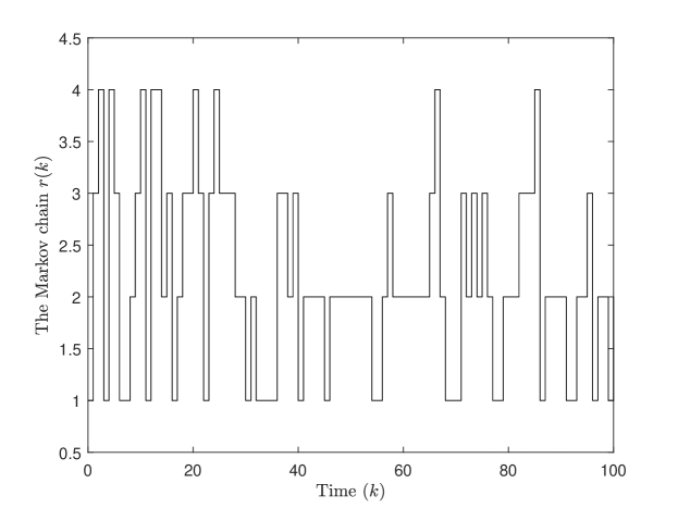
Figure 1: Markov switching between four modes

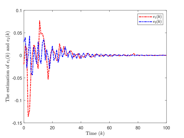
Figure 2: Estimation error $e_{1}(k)$ and $e_{2}(k)$.

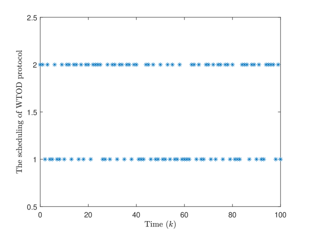
Figure 3: The scheduling of WTOD protocol.

5 Conclusions

References

• (1) Hongchao Li, Zhiqiang Zuo, Yijing Wang (2016) Event triggered control for Markovian jump systems with partially unknown transition probabilities and actuator saturation. Journal of the Franklin Institute 353(8): 1848–1861
• (2) Jamal Daafouz, Pierre Riedinger, Claude Iung (2002) Stability analysis and control synthesis for switched systems: a switched Lyapunov function approach. IEEE Transactions on Automatic Control 47(11): 1883–1887
• (3) Mingang Hua, Dandan Zheng, Feiqi Deng (2018) Partially mode-dependent $l_{2}$-$l_{\infty}$ filtering for discrete-time nonhomogeneous Markov jump systems with repeated scalar nonlinearities. Information Sciences 451–452: 223–239
• (4) Kun Liang, Mingcheng Dai, Hao Shen, Jing Wang, Zhen Wang, Bo Chen (2018) $L_{2}$-$L_{\infty}$ synchronization for singularly perturbed complex networks with semi-Markov jump topology. Applied Mathematics and Computation 321(16): 450–462
• (5) Deyin Yao, Ming Liu, Renquan Lu, Yong Xu, Qi Zhou (2018) Adaptive sliding mode controller design of Markov jump systems with time-varying actuator faults and partly unknown transition probabilities. Nonlinear Analysis: Hybrid Systems 28: 105–122
• (6) Mouquan Shen (2013) $H_{\infty}$ filtering of continuous Markov jump linear system with partly known Markov modes and transition probabilities. Journal of the Franklin Institute 350(10): 3384–3399
• (7) Wenxia Cui, Shaoyuan Sun, Jianan Fang, Yulong Xu, Lingdong Zhao (2014) Finite-time synchronization of Markovian jump complex networks with partially unknown transition rates. Journal of the Franklin Institute 351(5): 2543–2561
• (8) Yanyan Yin, Jiangbin Shi, Fei Liu, Yanqing Liu (2020) Robust fault detection of singular Markov jump systems with partially unknown information. Information Sciences 537: 368–379
• (9) Lixian Zhang, El-Kébir Boukas, James Lam (2008) Analysis and synthesis of Markov jump linear systems with time-varying delays and partially known transition probabilities. IEEE Transactions on Automatic Control 53(10): 2458–2464
• (10) Guoliang Wang (2011) Partially mode-dependent design of filter for stochastic Markovian jump systems with mode-dependent time delays. Journal of Mathematical Analysis and Applications 383(2): 573–584
• (11) Huihui Ji, He Zhang, Tian Senping (2017) Reachable set estimation for inertial Markov jump BAM neural network with partially unknown transition rates and bounded disturbances. Journal of the Franklin Institute 354(15): 7158–7182
• (12) Yufei Liu, Bo Shen, Qi Li (2019) State estimation for neural networks with Markov-based nonuniform sampling: the partly unknown transition probability case. Neurocomputing 357: 261–270
• (13) Zidong Wang, Yao Wang, Yurong Liu (2010) Global synchronization for discrete-time stochastic complex networks with randomly occurred nonlinearities and mixed time delays. IEEE Transactions on Neural Networks 21: 11–25
• (14) Zhongyi Zhao, Zidong Wang, Lei Zou, Hongjian Liu (2018) Finite-horizon $H_{\infty}$ state estimation for artificial neural networks with component-based distributed delays and stochastic protocol. Neurocomputing 321: 169–177
• (15) Hongjian Liu, Zidong Wang, Weiyin Fei, Hongli Dong (2021) On state estimation for discrete time-delayed memristive neural networks under the WTOD Protocol: a resilient set-membership approach. IEEE Transactions on Systems, Man and Cybernetics:Systems
• (16) Yun Chen, Weixing Zheng (2015) $L_{2}$-$L_{\infty}$ filtering for stochastic Markovian jump delay systems with nonlinear perturbations. Signal Processing 109: 154–164
• (17) Yuxuan Shen, Zidong Wang, Bo Shen, Fuad E. Alsaadi, Abdullah M. Dobaie (2020) $l_{2}$-$l_{\infty}$ state estimation for delayed artificial neural networks under high-rate communication channels with Round-Robin protocol. Neural Networks 124: 170–179
• (18) Wei Qian, Yonggang Chen, Yurong Liu, Fuad E. Alsaadi (2018) Further results on $L_{2}$-$L_{\infty}$ state estimation of delayed neural networks. Neurocomputing 273: 509–515
• (19) Wei Qian, Yujie Li, Yonggang Chen, Yi Yang (2019) Delay-dependent $L_{2}$-$L_{\infty}$ state estimation for neural networks with state and measurement time-varying delays. Neurocomputing 331: 434–442
• (20) Wei Qian, Yalong Li, Yunji Zhao, Yonggang Chen (2020) New optimal method for $L_{2}$-$L_{\infty}$ state estimation of delayed neural networks. Neurocomputing 415: 258–265
• (21) Hao Shen, Mengping Xing, Zhengguang Wu, Jinde Cao, Tingwen Huang (2021) $l_{2}$-$l_{\infty}$ state estimation for persistent dwell-time switched coupled networks subject to Round-Robin protocol. IEEE Transactions on Neural Networks and Learning Systems 32(5): 2002–2014
• (22) Jiahui Li, Zidong Wang, Hongli Dong, Weiyin Fei (2020) Delay-distribution-dependent state estimation for neural networks under stochastic communication protocol with uncertain transition probabilities. Neural Networks 130: 143–151
• (23) Lei Zou, Zidong Wang, Qinglong Han, Donghua Zhou (2017) Ultimate boundedness control for networked systems with try-once-discard protocol and uniform quantization effects. IEEE Transactions on Automatic Control 62(12): 6582–6588
• (24) Yue Long, Ju H.Park, Dan Ye (2019) Frequency-dependent fault detection for networked systems under uniform quantization and try-once-discard protocol. International Journal of Robust and Nonlinear Control 30(2): 787–303
• (25) Lei Liu, Yiwen Wang, Lifeng Ma, Jie Zhang, Yuming Bo (2018) Robust finite-horizon filtering for nonlinear time-delay Markovian jump systems with weighted try-once-discard protocol. Systems Science & Control Engineering 6(1): 180–194
• (26) Lei Zou, Zidong Wang, Huijun Gao (2016) Set-membership filtering for time-varying systems with mixed time-delays under Round-Robin and weighted try-once-discard protocols. Automatica 74: 341–348
• (27) Jin Zhang, Chen Peng (2019) Networked $H_{\infty}$ filtering under a weighted TOD protocol. Automatica 107: 333–341
• (28) Yuxuan Shen, Zidong Wang, Bo Shen, Fawaz E. Alsaadi, Fuad E. Alsaadi (2020) Fusion estimation for multi-rate linear repetitive processes under weighted try-once-discard protocol. Information Fusion 55: 281–291
• (29) Yamei Ju, Guoliang Wei, Derui Ding, Shuai Liu (2020) A novel fault detection method under weighted try-once-discard scheduling over sensor networks. IEEE Transactions on Control of Network Systems 7(3):1489–1499
• (30) Muhammad Shamrooz Aslam, Xisheng Dai (2020) Event-triggered based $L_{2}$-$L_{\infty}$ filtering for multiagent systems with Markovian jumping topologies under time-varying delays. Nonlinear Dyn 99: 2877–2892
• (31) Weilu Chen, Jun Hu, Xiaoyang Yu, Dongyan Chen, Junhua Du (2020) Robust fault detection for nonlinear discrete systems with data drift and randomly occurring faults under weighted try-once-discard protocol. Circuits, Systems, and Signal Processing 39: 111–137