SCATTERING BY A PERFORATED SANDWICH PANEL:
METHOD OF RIEMANN SURFACES

Abstract

The model problem of scattering of a sound wave by an infinite plane structure formed by a semi-infinite acoustically hard screen and a semi-infinite sandwich panel perforated from one side and covered by a membrane from the other is exactly solved. The model is governed by two Helmholtz equations for the velocity potentials in the upper and lower half-planes coupled by the Leppington effective boundary condition and the equation of vibration of a membrane in a fluid. Two methods of solution are proposed and discussed. Both methods reduce the problem to an order-2 vector Riemann-Hilbert problem. The matrix coefficients have different entries, have the Chebotarev-Khrapkov structure and share the same order-4 characteristic polynomial. Exact Wiener-Hopf matrix factorization requires solving a scalar Riemann-Hilbert on an elliptic surface and the associated genus-1 Jacobi inversion problem solved in terms of the associated Riemann $\theta$-function. Numerical results for the absolute value of the total velocity potentials are reported and discussed.

1 Introduction

The effect of perforation on the transmission of sound waves through single-leaf and double-leaf panels was analyzed in (1), (2). When an elastic double-leaf honeycomb panel is perforated from one or both sides the transmission of sound is significantly reduced (3). Leppington (3) applied the method of matched asymptotic expansions to analyze this effect for an infinite honeycomb cellular structure in the cases of acoustically hard or acoustically transparent cell walls. One of the main results of this work is the derivation of the effective boundary conditions. In particular, in the case of cells with acoustically hard walls, the effective boundary condition on the panel surface $S=\{x\in I,y=0\}$ has the form

$$\psi_{1y}-\psi_{0y}+k\tau\psi_{1}=0,\quad(x,y)\in S,$$ (1.1)

where $\psi_{0}$ and $\psi_{1}$ are the velocity potentials in the lower and upper half-planes, $\psi_{jy}$ is the normal derivative of $\psi_{j}$, $k$ is the wave number, and $\tau$ is a parameter that accounts for perforations. The condition (1.1) is to be complemented by the classical boundary condition

$$D_{x}[\psi_{0y}]-\alpha(\psi_{1}-\psi_{0})=0,\quad(x,y)\in S,$$ (1.2)

where $D_{x}$ is the differential operator with respect to $x$ of order 2 or 4 depending whether the lower unperforated skin of the elastic structure is a membrane or an elastic plate and $\alpha$ is a parameter.

The model problem of scattering of a plane sound wave by an infinite plane structure formed by a semi-infinite acoustically hard screen and semi-infinite honeycomb elastic panel with acoustically hard walls perforated from one side was reduced (4) to a Riemann-Hilbert problem for two pairs of functions. This work does not factorize the matrix coefficient. Instead, it applies the asymptotic method of small $\tau$ with the leading-order term determined by the decoupled problem.

The vector Riemann-Hilbert (4) was analyzed (5) by the method of factorization on a Riemann surface (6), (7). It was shown that the matrix coefficient of the vector Riemann-Hilbert problem has the Chebotarev-Khrapkov structure (8), (9) with the characteristic polynomial $f(s)$ of degree 8. The Khrapkov methodology is applicable when $degf(s)\leq 2$. For a particular case of the Chebotarev-Khrapkov matrix and when $\deg f(s)=4$, a method of elliptic functions eliminating the essential singularity at infinity was proposed in (10). A numerical approach of Padé approximants for factorization of the Chebotarev–Khrapkov matrix was developed in (11). If $\deg f(s)=8$, then the exact representation of the Wiener-Hopf matrix factors includes exponents of functions having an order-3 pole at infinity and therefore has an unacceptable essential singularity. This singularity was eliminated (5) by reducing the matrix factorization problem to a scalar Riemann-Hilbert problem on a hyperelliptic surface (12) and solving the associated genus-3 Jacobi inversion problem (13), (14). The solution (5) was designed for the case of real wave numbers. In this case all eight branch points lie on the same circle and are symmetric with respect to the origin. That is why the brunch cuts and $A$- and $B$ - cross-sections are two-sided arcs of a circle. The full solution of the model problem requires to determine two unknown constants by satisfying the additional conditions, to analyze the behavior of the Wiener-Hopf matrix factors at infinity, and based on the solution obtained develop an efficient numerical procedure for the velocity potentiails. These aspects were not a scope of the investigation (5).

In this work we analyze the model problem of scattering of a plane sound wave by a structure similar to the one considered in (4), (5). The only one difference is that the lower skin of the structure is a membrane, not a thin plate. Mathematically, this means that instead of the fourth order differential operator $D_{x}$ in (1.2) we have a second order operator. We aim to derive the full solution, find unknown constants, analyze the behavior of the matrix factors at infinity and obtain numerical results. In Section 2, we formulate the model problem and write down the governing boundary value problem for two Helmholts equations coupled by the boundary conditions. We apply the Laplace transform and convert the problem into an order-2 vector Riemann-Hilbert problem in Section 3. We show that the problem of matrix factorization is equivalent to a scalar Riemann-Hilbert problem on an elliptic surface. To eliminate the essential singularity of the factors at infinity, we solve a genus-1 Jacobi inversion problem in terms of the Riemann $\theta$-function. At the end of Section 3, we compute the partial indices of factorization and show that they are stable. In Section 4, we propose another method of reduction of the model problem to a vector Riemann-Hilbert problem in order to understand if the method has an advantage over the method applied in Section 3. Section 5 presents numerical results for the velocity potentials obtained on the basis of the solution derived in Section 3.

2 Formulation

Suppose that a semi-infinite sandwich panel is attached to a semi-infinite acoustically rigid screen (Fig. 1). The upper side of the panel $M_{1}=\{0<x<\infty,y=d\}$ is perforated, while the lower side $M_{0}=\{0<x<\infty,y=0\}$ is a smooth membrane. The unperforated and perforated skins are linked by cells whose sides are assumed to be acoustically hard. The rigid screen $S=\{-\infty<x<0,y=0\}$ and the lower side of the sandwich panel are clamped, and without loss of generality, the displacement is equal to zero at the junction point $x=0$, $y=0$.

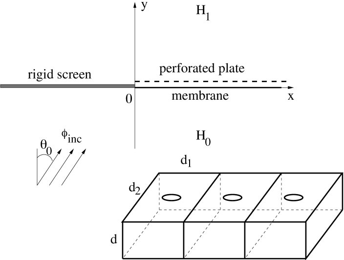
Figure 1: Sandwich panel attached to an acoustically rigid screen

Compressible fluid of wave speed $c$ occupies the regions outside the sandwich panel and the screen. The system is excited by a plane wave of incident velocity potential

$$\mathop{\rm Re}\nolimits\{\phi_{inc}e^{-i\omega t}\}=\mathop{\rm Re}\nolimits\{e^{ik(x\sin\theta_{0}+y\cos\theta_{0}}e^{-i\omega t}\},\quad y<0,$$ (2.1)

where $\theta_{0}\in(-\pi/2,\pi/2)$, $k=\frac{\omega}{c}$ is the acoustic wave number, $k=k_{1}+ik_{2}$, $0<k_{2}<<k_{1}$, and $\omega$ is the radian frequency. The velocity potentials $\psi_{0,1}e^{-i\omega t}$ in the lower and upper half-planes ${{H}_{0}}$ and ${{H}_{1}}$ satisfy the Helmholtz equation

$$\left(\frac{\partial^{2}}{\partial x^{2}}+\frac{\partial^{2}}{\partial x^{2}}+k^{2}\right)\psi_{j}(x,y)=0,\quad(x,y)\in{{H}_{j}},\quad j=0,1.$$ (2.2)

The two potentials satisfy the standard acoustically hard boundary conditions

$$\frac{\partial\psi_{0}}{\partial y}=\frac{\partial\psi_{1}}{\partial y}=0,\quad x<0,\quad y=0.$$ (2.3)

The surface deflection $\eta_{0}e^{-i\omega t}$ of the membrane $M_{0}$ and the pressure fluctuation $p_{j}e^{-i\omega t}$ are given in terms of the potentials by the relations

$$\eta_{0}=\frac{i}{\omega}\frac{\partial\psi_{0}}{\partial y},\quad p_{j}=i\omega\rho_{f}\psi_{j},\quad j=0,1,$$ (2.4)

where $\rho_{f}$ is the mean density of the fluid. The deflection of the membrane responds to the total surface pressure according to the linearized equation (15)

$$m_{0}\frac{\partial^{2}}{\partial t^{2}}\left(\eta_{0}e^{-i\omega t}\right)=T\frac{\partial^{2}}{\partial x^{2}}\left(\eta_{0}e^{-i\omega t}\right)-(p_{1}-p_{0})e^{-i\omega t},\quad y=0,\quad x>0.$$ (2.5)

Here, $m_{0}$ is the mass per unit area of the membrane, $T$ is the tension per unit length. Equivalently, this boundary condition can be written in the form

$$\frac{\partial^{3}\psi_{0}}{\partial x^{2}\partial y}+\mu^{2}\frac{\partial\psi_{0}}{\partial y}-\alpha(\psi_{1}-\psi_{0})=0,\quad y=0,\quad x>0,$$ (2.6)

where

$$\mu=\sqrt{\frac{m_{0}}{T}}\omega,\quad\alpha=\frac{\rho_{f}\omega^{2}}{T}.$$ (2.7)

The second boundary condition of the sandwich panel is the Leppington (3) effective boundary condition

$$\frac{\partial\psi_{1}}{\partial y}-\frac{\partial\psi_{0}}{\partial y}+k\tau\psi_{1}=0,\quad y=0,\quad x>0,$$ (2.8)

where

$$\tau=\frac{kd}{1-k^{2}V/(2a)},$$ (2.9)

where $a$ is the aperture radius and $V$ is the cell volume, $V=d_{1}d_{2}d$. In the derivation (3) of the boundary condition (2.8), it is assumed that the wavelength is large compared with the spacing parameters $d_{1}$, $d_{2}$ and $d$ (Fig. 1), so that $|k|d_{1}<<1$, $|k|d_{2}<<1$, and $|k|d<<1$. Since $|k|d$ is small, the boundary condition can be applied at $y=0$ to leading order. The parameter $\tau$ is dimensionless, while the parameters $\mu$ and $\alpha$ have dimensions $L^{-1}$ and $L^{-3}$, respectively, with $L$ measured in units of length. The condition $\tau=\infty$, an analog of the Helmholtz resonance (16) condition, gives the critical value $k_{res}$ (3) of the wave number

$$k_{res}=\sqrt{\frac{2a}{V}}.$$ (2.10)

For complex wave numbers $k$, this condition is never satisfied. However, it is clear that when $\mathop{\rm Re}\nolimits k>>\mathop{\rm Im}\nolimits k>0$ and $|k|\to k_{res}$, $|\tau|\to\infty$.

It is convenient to introduce a reflected wave of potential $\phi_{ref}=e^{ik(x\sin\theta_{0}-y\cos\theta_{0})}$ and scattering potentials $\phi_{0}$ and $\phi_{1}$. Then the total velocity potentials are expressed through the incident, reflected and scattering potentials by

$$\psi_{0}=\phi_{inc}+\phi_{ref}+\phi_{0},\quad y<0;\quad\psi_{1}=\phi_{1},\quad y>0.$$ (2.11)

The scattering potentials satisfy the Helmholtz equation

$$\left(\frac{\partial^{2}}{\partial x^{2}}+\frac{\partial^{2}}{\partial x^{2}}+k^{2}\right)\phi_{j}(x,y)=0,\quad(x,y)\in{{H}_{j}},\quad j=0,1,$$ (2.12)

and the following boundary conditions:

$$\frac{\partial\phi_{0}}{\partial y}=\frac{\partial\phi_{1}}{\partial y}=0,\quad x<0,\quad y=0,$$

$$\frac{\partial^{3}\phi_{0}}{\partial x^{2}\partial y}+\mu^{2}\frac{\partial\phi_{0}}{\partial y}-\alpha(\phi_{1}-\phi_{0})=-2\alpha e^{ikx\sin\theta_{0}},\quad x>0,\quad y=0,$$

$$\frac{\partial\phi_{1}}{\partial y}-\frac{\partial\phi_{0}}{\partial y}+k\tau\phi_{1}=0,\quad x>0,\quad y=0.$$ (2.13)

It is also required that the scattering potentials $\phi_{0}$ and $\phi_{1}$ satisfy an outgoing wave radiation condition as $x^{2}+y^{2}\to\infty$.

3 Vector Riemann-Hilbert problem

3.1 Derivation based on the Laplace transform of the velocity potentials

To reduce the boundary value problem (2.12), (2.13) to a vector Riemann-Hilbert problem (known also as a matrix Wiener-Hopf problem), we introduce the Laplace transforms of the velocity potentials

$$\Phi_{j+}(s;y)=\int_{0}^{\infty}\phi_{j}(x,y)e^{isx}dx,\quad\Phi_{j-}(s;y)=\int_{-\infty}^{0}\phi_{j}(x,y)e^{isx}dx.$$ (3.1)

Their sums $\Phi_{j}(s;y)=\Phi_{j+}(s;y)+\Phi_{j-}(s;y)$ satisfy the equations

$$\left[\frac{d^{2}}{dy^{2}}-(s^{2}-k^{2})\right]\Phi_{j}(s;y)=0,\quad j=0,1.$$ (3.2)

Fix a single branch of the function $\gamma^{2}(s)=(s^{2}-k^{2})$ in the $s$-plane cut along the line joining the branch points $k$ and $-k$ and passing through the infinite point. Denote by $\theta_{*}=\arg k\in(0,\frac{\pi}{2})$ and select

$$-\pi+\theta_{*}\leq\theta_{+}\leq\pi+\theta_{*},\quad-2\pi+\theta_{*}\leq\theta_{-}\leq\theta_{*},$$ (3.3)

where $\theta_{\pm}=\arg(s\pm k)$. Then $\gamma(0)=-ik$ and $\mathop{\rm Re}\nolimits\gamma(s)>0$ on $L=(-\infty+i\kappa_{0},\infty+i\kappa_{0})$, $\kappa_{0}\in(-k_{2}\sin\theta_{0},k_{2})$. On disregarding the solution exponentially growing at infinity we write the general solution of equation (3.2)

$$\Phi_{0}(s,y)=A_{0}(s)e^{\gamma y},\quad y<0,\quad\Phi_{1}(s,y)=A_{1}(s)e^{-\gamma y},\quad y>0.$$ (3.4)

Applying the Laplace transforms (3.1) to the boundary conditions (2.13) gives four equations. They are

$$\frac{d}{dy}\Phi_{0-}(s;0)=0,\quad\frac{d}{dy}\Phi_{1-}(s;0)=0,$$

$$\frac{d}{dy}\Phi_{1+}(s;0)-\frac{d}{dy}\Phi_{0+}(s;0)+k\tau\Phi_{1+}(s;0)=0,$$

$$(\mu^{2}-s^{2})\frac{d}{dy}\Phi_{0+}(s;0)-\alpha\Phi_{1+}(s;0)+\alpha\Phi_{0+}(s;0)=N-\frac{2\alpha i}{s+k\sin\theta_{0}}.$$ (3.5)

Here, we used the fact that, owing to the continuity of the displacements at the point $x=0$,

$$\lim_{x\to 0^{+}}\frac{d}{dy}\phi_{0}(x;0)=0,$$ (3.6)

and denoted $N=\frac{d^{2}}{dxdy}\phi_{0}(0^{+};0)$ ($N$ is a free constant at this stage). On fixing $y=0$ in the general solutions defined by (3.4) and their derivatives and also employing the first two equations in the system (3.6) we find

$$\Phi_{j+}(s;0)+\Phi_{j-}(s;0)=A_{j}(s),\quad A_{j}(s)=\frac{(-1)^{j}}{\gamma(s)}\frac{d}{dy}\Phi_{j+}(s;0).$$ (3.7)

Analysis at infinity of the fourth equation in (3.5) and equations (3.7) shows that

$$\frac{d}{dy}\Phi_{0+}(s;0)=O(s^{-2}),\quad A_{0}(s)=O(s^{-3}),\quad A_{1}(s)=O(s^{-2}),\quad s\to\infty.$$ (3.8)

As for the asymptotics at infinity of the other functions in the system (3.5), they ensue from the Laplace representations (3.1) and the asymptotics (3.8). We have

$$\Phi_{j\pm}(s;0)=O(s^{-1}),\quad s\in{{C}^{\pm}},\quad j=0,1,\quad\frac{d}{dy}\Phi_{1+}(s;0)=O(s^{-1}),\quad s\in{{C}^{+}},\quad s\to\infty,$$

$$\Phi_{0+}(s;0)+\Phi_{0-}(s;0)=O(s^{-3}),\quad\Phi_{1+}(s;0)+\Phi_{1-}(s;0)=O(s^{-2}),\quad|s|\to\infty,\quad s\in L.$$ (3.9)

Now, the relations (3.7) enable us to eliminate the derivatives $\frac{d}{dy}\Phi_{j+}(s;0)$ from the third and fourth equations of the system (3.5) and obtain

$$[(\mu^{2}-s^{2})\gamma(s)+\alpha]\Phi_{0+}(s;0)-\alpha\Phi_{1+}(s;0)+(\mu^{2}-s^{2})\gamma(s)\Phi_{0-}(s;0)=N-\frac{2\alpha i}{s+k\sin\theta_{0}},$$

$$-\gamma(s)\Phi_{0+}(s;0)+(k\tau-\gamma)\Phi_{1+}(s;0)-\gamma(s)\Phi_{0-}(s;0)-\gamma(s)\Phi_{1-}(s;0)=0.$$ (3.10)

To rewrite this system in the matrix-vector form, we denote $\Phi_{j}^{\pm}(s)=\Phi_{j\pm}(s,0)$ and introduce the vectors

$$\Phi^{\pm}(s)=\left(\begin{array}[]{c}\Phi_{0}^{\pm}(s)\\ \Phi_{1}^{\pm}(s)\\ \end{array}\right),$$

$$g(s)=\frac{1}{\gamma(s)(s^{2}-\mu^{2})}\left(N-\frac{2\alpha i}{s+k\sin\theta_{0}}\right)\left(\begin{array}[]{c}-1\\ 1\end{array}\right),$$ (3.11)

and the matrix

$$G(s)=\left(\begin{array}[]{cc}b(s)+c(s)l(s)&c(s)m\\ c(s)m&b(s)-c(s)l(s)\end{array}\right),$$ (3.12)

where $b(s)$ and $c(s)$ are Hölder functions on the contour $L$, $l(s)$ is a polynomial and $m$ is a constant given by

$$b(s)=1-\frac{1}{\gamma(s)}\left(\frac{k\tau}{2}+\frac{\alpha}{s^{2}-\mu^{2}}\right),\quad c(s)=\frac{k\tau}{2\gamma(s)(s^{2}-\mu^{2})},$$

$$l(s)=s^{2}-\mu^{2},\quad m=\frac{2\alpha}{k\tau}.$$ (3.13)

In these notations, the system (3.10) can be reformulated as the following vector Riemann-Hilbert problem of the theory of analytic functions.

Find two vectors $\Phi^{+}(s)$ and $\Phi^{-}(s)$ analytic in the upper and lower half-planes ${{C}^{+}}$ and ${{C}^{-}}$, respectively, Hölder-continuous up to the contour $L$, such that their limit values on the boundary satisfy the vector equation

$$G(t)\Phi^{+}(t)+\Phi^{-}(t)=g(t),\quad t\in L.$$ (3.14)

The solution vanishes at infinity, $\Phi^{\pm}(s)=O(s^{-1})$, $s\to\infty$, $s\in{{C}^{\pm}}$, and

$$\Phi_{0}^{+}(t)+\Phi_{0}^{-}(t)=O(t^{-3}),\quad\Phi_{1}^{+}(t)+\Phi_{1}^{-}(t)=O(t^{-2}),\quad|t|\to\infty,\quad t\in L.$$ (3.15)

Also, due to the condition (3.6),

$$\int_{L}\gamma(t)[\Phi^{+}_{0}(t)+\Phi^{-}_{0}(t)]dt=0.$$ (3.16)

3.2 Matrix factorization

The matrix coefficient $G(s)$ of the vector Riemann-Hilbert problem is a Chebotarev-Khrapkov matrix (8), (9). Its characteristic polynomial is a degree-4 polynomial

$$f(s)=l^{2}(s)+m^{2}=(s^{2}-\mu^{2})^{2}+m^{2}.$$ (3.17)

In this case the problem of factorization reduces to a scalar Riemann-Hilbert problem on a two-sheeted genus-1 Riemann surface ${\cal R}$ of the algebraic function $w^{2}=f(s)$. Fix a single branch of this function by the condition $f^{1/2}(s)\sim s^{2}$, $s\to\infty$, in the plane $\hat{{C}}$ cut along the segments $\Gamma_{1}=[s_{1},s_{2}]$ and $\Gamma_{2}=[-s_{2},-s_{1}]$. Here, $\pm s_{1}$ and $\pm s_{2}$ are the four zeros of the function $f(s)$, $s_{1}^{2}=\mu^{2}+im$, $s_{2}^{2}=\mu^{2}-im$, $s_{1}$ and $s_{2}$ are the zeros lying in the second and first quadrant, respectively (Fig. 2).

Figure 2: The cuts $\Gamma_{1}$ and $\Gamma_{2}$ and the canonical cross-sections a and b.

Denote the two sheets of the surface ${\cal R}$ glued along the cuts $\Gamma_{1}$ and $\Gamma_{2}$ by ${C}_{1}$ and ${C}_{2}$. Let $w=f^{1/2}(s)$, $(s,w)\in{{C}_{1}}$ and $w=-f^{1/2}(s)$, $(s,w)\in{{C}_{2}}$.

A meromorphic solution of the factorization problem

$$G(t)=X^{+}(t)[X^{-}(t)]^{-1}=[X^{-}(t)]^{-1}X^{+}(t),\quad t\in L,$$ (3.18)

the matrix $X(s)$ and its inverse, has the form (6), (7), (5)

$$X(s)=F(s,w)B(s,w)+F(s,-w)B(s,-w),$$

$$[X(s)]^{-1}=\frac{B(s,w)}{F(s,w)}+\frac{B(s,-w)}{F(s,-w)},$$ (3.19)

where

$$B(s,w)=\frac{1}{2}\left(I+\frac{A(s)}{w}\right),\quad A(s)=\left(\begin{array}[]{cc}l(s)&m\\ m&-l(s)\end{array}\right).$$ (3.20)

The function $F(s,w)$ solves the following scalar Riemann-Hilbert problem on the contour ${\cal L}=L_{1}\cup L_{2},$ where $L_{1}\subset{C}_{1}$ and $L_{2}\subset{C}_{2}$ are two copies of the contour $L$.

Find a function $F(s,w)$ piece-wise meromorphic on the surface ${\cal R}$, Hölder-continuous up to the contour ${\cal L}$, bounded at the two infinite points of the surface ${\cal R}$, such that the limit values of the function $F(s,w)$ on the contour ${\cal L}$ satisfy the relation

$$F^{+}(t,\xi)=\lambda(t,\xi)F^{-}(t,\xi),\quad(t,\xi)\in{\cal L},$$ (3.21)

where $\xi=w(t)$, $\lambda(t,\xi)=\lambda_{j}(t)$ on ${C}_{j}$, $j=1,2$, and $\lambda_{1}(t)=b(t)+c(t)f^{1/2}(t)$ and $\lambda_{2}(t)=b(t)-c(t)f^{1/2}(t)$ are the two eigenvalues of the matrix $G(t)$.

It is directly verified that the increments of the arguments of the eigenvalues $\lambda_{1}(t)$ and $\lambda_{2}(t)$ when $t$ traverses the contour $L$ from $-\infty+i\kappa_{0}$ to $+\infty+i\kappa_{0}$ are equal to zero. Therefore the general solution of the problem (3.21) has the form

$$F(s,w)=e^{\chi(s,w)},\quad(s,w)\in{\cal R},$$ (3.22)

where

$$\chi(s,w)=\frac{1}{2\pi i}\int_{\cal L}\log\lambda(t,\xi)dW+\int_{\Gamma}dW+m_{a}\int_{\rm{\bf a}}dW+m_{b}\int_{\rm{\bf b}}dW,$$ (3.23)

$dW$ is the Weierstrass analog of the Cauchy kernel on an elliptic surface,

$$dW=\frac{w+\xi}{2\xi}\frac{dt}{t-s}$$ (3.24)

and $\Gamma$ is a contour on the surface ${\cal R}$ whose starting point $q_{0}$ is fixed arbitrarily say, $q_{0}=(\zeta_{0},f^{1/2}(\zeta_{0}))\in{{C}_{1}}$, while the terminal point $q_{1}=(\zeta_{1},w(\zeta_{1}))\in{\cal R}$ cannot be fixed a priori and has to be determined. In formula (3.23), there are two more undetermined quantities, $m_{a}$ and $m_{b}$. They are integers and have also to be determined. The contours of integration ${\rm\bf a}$ and ${\rm\bf b}$ are canonical cross-sections of the surface ${\cal R}$ (Fig. 2). The cross-section ${\rm\bf a}={\rm\bf a^{+}}\cup{\rm\bf a^{-}}$ is a two-sided loop, ${\rm\bf a^{+}}\in{{C}_{1}}$ and ${\rm\bf a^{-}}\in{{C}_{2}}$. The closed contour ${\rm\bf b}$ consists os the segment $[s_{2},-s_{1}]\in{{C}_{1}}$ and the segment $[-s_{1},s_{2}]\in{{C}_{2}}$ (the dashed line in Fig.2). The loop ${\rm\bf a}$ intersects the loop ${\rm\bf b}$ at the branch point $s_{2}$ from left to right. Note that the contour $\Gamma$ has to be chosen such that it intersects neither the contour ${\rm\bf a}$ no the contour ${\rm\bf b}$.

Because of the logarithmic singularities of the second integral in (3.23) at the endpoints of the contour $\Gamma$ the solution $F(s,w)$ has a simple pole at the point $q_{0}\in{{C}_{1}}$ and a simple zero at the point $q_{1}\in{\cal R}$. The kernel $dW$ has an order-2 pole at the infinite points of the surface. That is why the solution $F(s,w)$ has unacceptable essential singularities at the infinite points. To remove them, we first rewrite $\chi(s,w)$ in the form

$$\chi(s,w)=\chi_{1}(s)+w\chi_{2}(s),$$ (3.25)

where

$$\chi_{1}(s)=\frac{1}{4\pi i}\int_{L}\frac{\log\Delta(t)dt}{t-s}+\frac{1}{2}\int_{\Gamma}\frac{dt}{t-s},$$

$$\chi_{2}(s)=\frac{1}{4\pi i}\int_{L}\frac{\log\epsilon(t)dt}{(t-s)f^{1/2}(t)}+\frac{1}{2}\left(\int_{\Gamma}+m_{a}\int_{{\bf a}}+m_{b}\int_{{\bf b}}\right)\frac{dt}{(t-s)\xi},$$

$$\Delta(t)=\lambda_{1}(t)\lambda_{2}(t),\quad\epsilon(t)=\frac{\lambda_{1}(t)}{\lambda_{2}(t)}.$$ (3.26)

The function $\chi(s,w)$ is bounded at infinity if and only if $w\chi_{2}(s)=O(1)$, $s\to\infty$, or, equivalently,

$$\frac{1}{2\pi i}\int_{L}\frac{\log\epsilon(t)dt}{f^{1/2}(t)}+\int_{\Gamma}\frac{dt}{\xi}+m_{a}\int_{{\bf a}}\frac{dt}{\xi}+m_{b}\int_{{\bf b}}\frac{dt}{\xi}=0.$$ (3.27)

If the function $\chi_{2}(s)$ satisfies this condition, then because of the identity

$$\frac{1}{t-s}=-\frac{1}{s}+\frac{t}{s(t-s)},$$ (3.28)

it admits an alternative representation

$$\chi_{2}(s)=\frac{1}{4\pi is}\int_{L}\frac{\log\epsilon(t)tdt}{(t-s)f^{1/2}(t)}+\frac{1}{2s}\left(\int_{\Gamma}+m_{a}\int_{{\bf a}}+m_{b}\int_{{\bf b}}\right)\frac{tdt}{(t-s)\xi}.$$ (3.29)

This formula is valid for all $s\neq 0$ and can be used for numerical calculations when $|s|>1$ instead of formula (3.26) that is more convenient when $|s|\leq 1$.

3.3 Jacobi inversion problem

The condition (3.27) is equivalent to a genus-1 Jacobi inversion problem. To show this, consider the abelian (elliptic) integral

$$\omega(q)=\int_{-s_{2}}^{q}\frac{ds}{w(s)},\quad q=(s,w(s)).$$ (3.30)

Then the third and fourth integrals in equation (3.27),

$${\cal A}=\int_{{\bf a}}\frac{ds}{w(s)}=2\int_{{\bf a}^{+}}\frac{ds}{f^{1/2}(s)},$$

$${\cal B}=\int_{{\bf b}}\frac{ds}{w(s)}=2\int_{s_{2}}^{-s_{1}}\frac{ds}{f^{1/2}(s)},$$ (3.31)

are the $A$- and $B$-periods of the integral $\omega(q)$. Thus the condition (3.27) constitute the following Jacobi inversion problem.

Find a point $q_{1}=(\zeta_{1},w_{1})\in{\cal R}$ and two integers $m_{a}$ and $m_{b}$ such that

$$\omega(q_{1})+m_{a}{\cal A}+m_{b}{\cal B}=d_{0},$$ (3.32)

where

$$d_{0}=\omega(q_{0})-\frac{1}{2\pi i}\int_{L}\frac{\log\epsilon(t)dt}{f^{1/2}(t)}.$$ (3.33)

By dividing equation (3.32) by ${\cal A}$ we arrive at the canonical form of the Jacobi problem

$$\hat{\omega}(q_{1})=e_{1}-k_{1}-m_{a}-m_{b}\hat{\cal B}\equiv e_{1}-k_{1}\quad(\rm{modulo\;the\;periods})$$ (3.34)

for the canonical abelian integral $\hat{\omega}(q)=\frac{\omega(q)}{{\cal A}}$. It has the unit $A$-period, while its $B$-period $\hat{\cal B}=\frac{{\cal B}}{{\cal A}}$ has a positive imaginary part, $\mathop{\rm Im}\nolimits\hat{\cal B}>0$. Here, $e_{1}=\frac{d_{0}}{{\cal A}}+k_{1}$ and $k_{1}$ is the Riemann constant of the surface $\tilde{\cal R}$ cut along the loops $\rm{\bf a}$ and $\rm{\bf b}$. It is computed in (17), $k_{1}=-\frac{1}{2}+\frac{1}{2}\hat{\cal B}$.

The unknown point $q_{1}=(\zeta_{1},w_{1})$ is the single zero of the genus-1 Riemann $\theta$-function

$${\cal F}(q)=\theta(\hat{\omega}(q)-e_{1})=\sum_{\nu=-\infty}^{\infty}\exp\{\pi i\hat{\cal B}\nu^{2}+2\pi i\nu[\hat{\omega}(q)-e_{1}]\}.$$ (3.35)

To find $\zeta_{1}$, consider the integral

$$M=\frac{1}{2\pi i}\int_{\partial\hat{\cal R}}\frac{d\log{\cal F}(q)}{s-i},$$ (3.36)

where $\partial\hat{\cal R}$ is the boundary of the surface ${\cal R}$ cut along the cross-section ${{\bf a}}$ only. The procedure we are going to apply is a modification of the method (9) that instead of the poles at the two points $i_{1}=(i,f^{1/2}(i))\in{{C}_{1}}$ and $i_{2}=(i,-f^{1/2}(i))\in{{C}_{2}}$ in (3.36) uses an integrand with two poles at the infinite points of the surface ${\cal R}$. Without loss we assume that ${\cal F}(i_{n})\neq 0$, $n=1,2$, and compute the integral $M$ by applying the theory of residues. We have

$$M=\frac{1}{\zeta_{1}-i}+\frac{{\cal F}^{\prime}(i_{1})}{{\cal F}(i_{1})}+\frac{{\cal F}^{\prime}(i_{2})}{{\cal F}(i_{2})}.$$ (3.37)

where the derivative of the Riemann $\theta$-function is a rapidly convergent series

$${\cal F}^{\prime}(q)=\frac{2\pi i(-1)^{n-1}}{{\cal A}f^{1/2}(s)}\sum_{\nu=-\infty}^{\infty}\nu\exp\{\pi i\hat{\cal B}\nu^{2}+2\pi i\nu[\hat{\omega}(q)-e_{1}]\},\quad q\in{{C}_{n}},\quad n=1,2.$$ (3.38)

The integral (3.36) can also be represented as a contour integral

$$M=\frac{1}{2\pi i}\left(\int_{{\bf a}^{+}}+\int_{{\bf a}^{-}}\right)\frac{d\log{\cal F}(q)}{s-i}=\frac{1}{2\pi i}\int_{{\bf a}}\frac{1}{s-i}[d\log{\cal F}^{+}(q)-d\log{\cal F}^{-}(q)],$$ (3.39)

where ${\bf a}^{+}$ and ${\bf a}^{-}$ have opposite directions and pointwise coincide with the loop ${\bf a}$ from the side of the sheets ${C}_{1}$ and ${C}_{2}$, respectively, while the positive direction of the loops ${\bf a}^{+}$ and ${\bf a}$ are chosen such that the exterior of the cut $[s_{1},s_{2}]$ on the first sheet is on the left. Using the relation between the boundary values of the Riemann $\theta$-function on the loop ${\bf a}$

$${\cal F}^{+}(p)={\cal F}^{-}(p)\exp\{\pi i\hat{\cal B}-2\pi ie_{1}+2\pi i\hat{\omega}^{+}(p)\},\quad p\in{\rm{\bf a}},$$ (3.40)

where

$$\hat{\omega}^{+}(p)=\lim_{q\to p,q\in{{C}_{1}}}\hat{\omega}(q),$$ (3.41)

we derive another formula for the integral $M$

$$M=\int_{{\bf a}}\frac{d\hat{\omega}^{+}(q)}{s-i}=\frac{2}{{\cal A}}\int_{[s_{1},s_{2}]^{+}}\frac{ds}{(s-i)f^{1/2}(s)}.$$ (3.42)

Combining formulas (3.37) and (3.42) and introducing the quantity

$${\cal J}=\frac{2}{{\cal A}}\int_{[s_{1},s_{2}]^{+}}\frac{ds}{(s-i)f^{1/2}(s)}-\frac{{\cal F}^{\prime}(i_{1})}{{\cal F}(i_{1})}-\frac{{\cal F}^{\prime}(i_{2})}{{\cal F}(i_{2})}$$ (3.43)

we find the parameter $\zeta_{1}$

$$\zeta_{1}=i+\frac{1}{{\cal J}}.$$ (3.44)

Evaluate now the abelian integral at the point $\zeta_{1}$ lying on the first and second sheets,

$$\hat{\omega}(\zeta_{1},\pm f^{1/2}(\zeta_{1}))=\pm\frac{1}{{\cal A}}\int_{-s_{2}}^{\zeta_{1}}\frac{ds}{f^{1/2}(s)}.$$ (3.45)

and denote

$$d_{\pm}=\frac{d_{0}}{{\cal A}}-\hat{\omega}(\zeta_{1},\pm f^{1/2}(\zeta_{1})).$$ (3.46)

Taking the imaginary and real parts of the complex equation (3.40) we determine the constants $m^{\pm}_{b}$ and $m^{\pm}_{a}$

$$m^{\pm}_{b}=\frac{\mathop{\rm Im}\nolimits d_{\pm}}{\mathop{\rm Im}\nolimits\hat{\cal B}},\quad m^{\pm}_{a}=\mathop{\rm Re}\nolimits d_{\pm}-\frac{\mathop{\rm Re}\nolimits\hat{\cal B}}{\mathop{\rm Im}\nolimits\hat{\cal B}}\mathop{\rm Im}\nolimits d_{\pm}.$$ (3.47)

If it turns out that both of the integers $m^{+}_{a}$ and $m_{b}^{+}$ are integers, then $m_{a}=m_{a}^{+}$, $m_{b}=m_{b}^{+}$, and the point $q_{1}\in{{C}_{1}}$. Otherwise, $m_{a}=m_{a}^{-}$, $m_{b}=m_{b}^{-}$ are integers, and $q_{1}\in{{C}_{2}}$.

3.4 Solution of the vector Riemann-Hilbert problem

On having factorized the matrix $G(t)=X^{+}(t)[X^{-}(t)]^{-1}=[X^{-}(t)]^{-1}X^{+}(t)$, $t\in L$, and eliminated the essential singularity of the factors $X^{\pm}(s)$ at infinity, we proceed with the solution of the vector Riemann-Hilbert problem (3.14) by rewriting the boundary relation as

$$X^{+}(t)\Phi^{+}(t)-N\Psi_{+}^{(1)}(t)-\Psi_{+}^{(2)}(t)=-X^{-}(t)\Phi^{-}(t)-N\Psi_{-}^{(1)}(t)-\Psi_{-}^{(2)}(t),\quad t\in L.$$ (3.48)

Here, $\Psi^{(n)}_{\pm}(t)$ are the limit values of the Cauchy integrals

$$\Psi^{(1)}(s)=\frac{1}{2\pi i}\int_{L}\frac{X^{-}(t)J}{\gamma(t)(t^{2}-\mu^{2})}\frac{dt}{t-s},\quad J=\left(\begin{array}[]{c}-1\\ 1\end{array}\right),$$

$$\Psi^{(2)}(s)=-\frac{\alpha}{\pi}\int_{L}\frac{X^{-}(t)J}{\gamma(t)(t^{2}-\mu^{2})(t+k\sin\theta_{0})}\frac{dt}{t-s},$$ (3.49)

defined by the Sokhotski-Plemelj formulas

$$\Psi_{\pm}^{(1)}(t)=\pm\frac{X^{-}(t)J}{2\gamma(t)(t^{2}-\mu^{2})}+P.V.\Psi^{(1)}(t),$$

$$\Psi_{\pm}^{(2)}(t)=\mp\frac{\alpha iX^{-}(t)J}{\gamma(t)(t^{2}-\mu^{2})(t+k\sin\theta_{0})}+P.V.\Psi^{(2)}(t),\quad t\in L.$$ (3.50)

By the continuity principle and the generalized Liouville’s theorem of the theory of analytic functions,

$$\pm X^{\pm}(s)\Phi^{\pm}(s)-N\Psi_{\pm}^{(1)}(s)-\Psi_{\pm}^{(2)}(s)=R(s),\quad s\in{{C}^{\pm}},$$ (3.51)

where $R(s)$ is a rational vector-function to be determined. Since the matrices $X^{\pm}(s)$ are bounded at infinity, while the vectors $\Phi^{\pm}(s)$, $\Psi_{\pm}^{(1)}(s)$ and $\Psi_{\pm}^{(2)}(s)$ behave as $s^{-1}\mbox{const}$ for large $s$, we have $R(s)=O(s^{-1})$, $s\to\infty$.

Show next that the rational vector-function $R(s)$ has a pole at the point $s=\zeta_{0}$. Indeed, due to the logarithmic singularity of the function $\chi(s,w)$ at the starting point $(\zeta_{0},f^{1/2}(\zeta_{0}))\in{{C}_{1}}$ of the contour $\Gamma$, the function $F(s,w)$ has a simple pole at this point and is bounded at the point $(\zeta_{0},-f^{1/2}(\zeta_{0}))\in{{C}_{2}}$,

$$F(s,w)\sim D_{0}(s-\zeta_{0})^{-1},\quad F(s,-w)=O(1),\quad s\to\zeta_{0},\quad(s,w)\in{{C}_{1}}.$$ (3.52)

Employing the first formula in (3.19) for the matrix $X(s)$ we obtain

$$X(s)\Phi(s)\sim\frac{D_{0}}{2(s-\zeta_{0})}\left[\left(1+\frac{l(\zeta_{0})}{f^{1/2}(\zeta_{0})}\right)\Phi_{0}(\zeta_{0})+\frac{m}{f^{1/2}(\zeta_{0})}\Phi_{1}(\zeta_{0})\right]\left(\begin{array}[]{c}1\\ \eta_{0}\end{array}\right),$$ (3.53)

where

$$\eta_{0}=\frac{m}{l(\zeta_{0})+f^{1/2}(\zeta_{0})}.$$ (3.54)

This enables us to find the vector $R(s)$. We have

$$R(s)=\frac{C}{s-\zeta_{0}}\left(\begin{array}[]{c}1\\ \eta_{0}\end{array}\right),$$ (3.55)

where $C$ is a free constant. By substituting this expression into equation (3.51) we get the solution of the vector Riemann-Hilbert problem (3.14)

$$\Phi^{\pm}(s)=\pm[X^{\pm}(s)]^{-1}\left[\frac{C}{s-\zeta_{0}}\left(\begin{array}[]{c}1\\ \eta_{0}\end{array}\right)+N\Psi_{\pm}^{(1)}(s)+\Psi_{\pm}^{(2)}(s)\right],\quad s\in{{C}^{\pm}}.$$ (3.56)

Now, the function $F(s,w)$ has a simple zero at the point $q_{1}\in{\cal R}$ caused by the logarithmic singularity of the function $\chi(s,w)$ at the terminal point of the contour $\Gamma$. If $q_{1}=(\zeta_{1},w_{1})\in{{C}_{1}}$, then $w_{1}=f^{1/2}(\zeta_{1})$ and

$$F(s,w)\sim D_{1}(s-\zeta_{1}),\quad F(s,-w)\sim D_{2},\quad(s,w)\in{{C}_{1}},\quad s\to\zeta_{1}.$$ (3.57)

Otherwise, is $q_{1}=(\zeta_{1},w_{1})\in{{C}_{2}}$, then $w_{1}=-f^{1/2}(\zeta_{1})$ and

$$F(s,w)\sim D_{2},\quad F(s,-w)\sim D_{1}(s-\zeta_{1}),\quad(s,w)\in{{C}_{1}},\quad s\to\zeta_{1}.$$ (3.58)

Here, $D_{1}$ and $D_{2}$ are nonzero constants. From the second formula in (3.19) for the inverse matrix $[X(s)]^{-1}$, it becomes evident that the matrix $[X(s)]^{-1}$ has a pole at the point $s=\zeta_{1}$. Since ${\rm rank}\,B(s,w)=1$, the vector-function $F(s,w)$ has a removable singularity at the point $s=\zeta_{1}$ if and only if

$$\Pi_{0}C+\Pi_{1}N=-\Pi_{2},$$ (3.59)

where

$$\Pi_{0}=\left(\frac{w_{1}+l(\zeta_{1})}{m}+\eta_{0}\right)\frac{1}{\zeta_{1}-\zeta_{0}},\quad\Pi_{1}=\frac{w_{1}+l(\zeta_{1})}{m}\Psi_{0}^{(1)}(\zeta_{1})+\Psi_{1}^{(1)}(\zeta_{1}),$$

$$\Pi_{2}=\frac{w_{1}+l(\zeta_{1})}{m}\Psi_{0}^{(2)}(\zeta_{1})+\Psi_{1}^{(2)}(\zeta_{1}),$$ (3.60)

and $\Psi_{0}^{(n)}(s)$ and $\Psi_{1}^{(n)}(s)$ ($n=1,2$) are the two components of the vectors $\Psi^{(n)}(s)$ given by (3.49). Equation (3.59) constitutes the first equation for the unknown constants $C$ and $N$.

The solution derived has to be restricted to the class of functions satisfying the conditions (3.15). To verify these conditions, we examine the asymptotics of the vectors $\Phi^{+}(t)$ and $\Phi^{-}(t)$ as $|t|\to\infty$, $t\in L$. We start with the analysis of the functions $\Delta(t)$ and $\epsilon(t)$. From formulas (3.13) and (3.26) we have

$$\Delta(t)=1-\frac{k\tau}{\gamma(t)}-\frac{2\alpha}{\gamma(t)(t^{2}-\mu^{2})}+\frac{k\tau\alpha}{\gamma^{2}(t)(t^{2}-\mu^{2})}=1-\frac{k\tau}{|t|}+O(t^{-3}),\quad|t|\to\infty,\quad t\in L,$$

$$\epsilon(t)=\frac{b(t)+c(t)f^{1/2}(t)}{b(t)-c(t)f^{1/2}(t)}=1+\frac{k\tau}{|t|}+O(t^{-2}),\quad|t|\to\infty,\quad t\in L,$$ (3.61)

By applying the Sokhotski-Plemelj formulas to the integral representations of the functions $\chi_{1}(s)$ and $\chi_{2}(s)$ given by (3.26) and (3.29) we deduce

$$\chi_{1}^{\pm}(t)=\pm\frac{\log\Delta(t)}{4}+\frac{1}{4\pi i}\int_{L}\frac{\log\Delta(t_{0})dt_{0}}{t_{0}-t}+\frac{1}{2}\int_{\Gamma}\frac{dt_{0}}{t_{0}-t},\quad t\in L,$$

$$f^{1/2}(t)\chi^{\pm}_{2}(t)=\pm\frac{\log\epsilon(t)}{4}+\frac{f^{1/2}(t)}{4\pi it}\int_{L}\frac{\log\epsilon(t_{0})t_{0}dt_{0}}{(t_{0}-t)f^{1/2}(t_{0})}$$

$$+\frac{f^{1/2}(t)}{2t}\left(\int_{\Gamma}+m_{a}\int_{{\bf a}}+m_{b}\int_{{\bf b}}\right)\frac{t_{0}dt_{0}}{(t_{0}-t)\xi(t_{0})},\quad t\in L\setminus\{0\}.$$ (3.62)

We focus our attention on the principal terms of the asymptotic expansions at infinity of the two functions in (3.62) and observe that

$$\chi_{1}^{\pm}(t)=\mp\frac{k\tau}{4|t|}+\frac{k\tau}{2\pi it}\log|t|+\frac{h_{1}}{t}+O(t^{-2}),\quad|t|\to\infty,\quad t\in L,$$

$$f^{1/2}(t)\chi^{\pm}_{2}(t)=h_{0}\pm\frac{k\tau}{4|t|}-\frac{k\tau}{2\pi it}\log|t|+\frac{h_{2}}{t}+O(t^{-2}),\quad|t|\to\infty,\quad t\in L,$$ (3.63)

where

$$h_{0}=-\frac{1}{2}\left(\int_{\Gamma}+m_{a}\int_{{\bf a}}+m_{b}\int_{{\bf b}}\right)\frac{tdt}{\xi(t)}$$ (3.64)

and $h_{1}$ and $h_{2}$ are some constants. Their values do not affect the asymptotics we aim to derive.

Next, by virtue of the relation (3.25) we can derive the asymptotics of the solution of the Riemann-Hilbert problem on the surface ${\cal R}$ as follows:

$$F^{\pm}(t,f^{1/2}(t))=e^{h_{0}}\left[1+\frac{h_{+}}{t}+O(t^{-2})\right],\quad|t|\to\infty,\quad t\in L,$$

$$F^{\pm}(t,-f^{1/2}(t))=e^{-h_{0}}\left[1\mp\frac{k\tau}{2|t|}+\frac{k\tau}{\pi it}\log|t|+\frac{h_{-}}{t}+O\left(\frac{\log^{2}|t|}{t^{2}}\right)\right],\quad|t|\to\infty,\quad t\in L,$$ (3.65)

where $h_{\pm}=h_{1}\pm h_{2}$. Substituting these expressions into formula (3.19) for the inverse matrix $[X(s)]^{-1}$ gives

$$[X^{\pm}(t)]^{-1}=\left(\begin{array}[]{cc}e^{-h_{0}}(1-h_{+}t^{-1})&0\\ 0&e^{h_{0}}[1-k\tau(\pi it)^{-1}\log|t|-h_{-}t^{-1}]+O(t^{-2}\log^{2}|t|)\end{array}\right)$$

$$\pm\frac{k\tau e^{h_{0}}}{2|t|}\left(\begin{array}[]{cc}0&0\\ 0&1\end{array}\right)+O\left(\frac{1}{t^{2}}\right),\quad|t|\to\infty,\quad t\in L,$$ (3.66)

The above result, together with formulas (3.50) and (3.56) enables us to derive formulas which describe the behavior of the solution $\Phi^{\pm}(t)$ of the vector Riemann-Hilbert problem on the contour $L$ when $|t|\to\infty$

$$\Phi^{\pm}(t)=\pm\frac{C_{0}}{t}\left(\begin{array}[]{cc}e^{-h_{0}}(1-h_{+}t^{-1})&0\\ 0&e^{h_{0}}[1-k\tau(\pi it)^{-1}\log|t|-h_{-}t^{-1}]+O(t^{-2}\log^{2}|t|)\end{array}\right)$$

$$+\frac{C_{0}k\tau e^{h_{0}}}{2|t|t}\left(\begin{array}[]{cc}0&0\\ 0&1\end{array}\right)+O\left(\frac{1}{t^{3}}\right),\quad|t|\to\infty,\quad t\in L,$$ (3.67)

where $C_{0}$ is a constant. From here we immediately get $\Phi^{+}_{0}(t)+\Phi^{-}_{0}(t)=O(t^{-3})$ and $\Phi^{+}_{1}(t)+\Phi^{-}_{1}(t)=O(t^{-2})$, $|t|\to\infty$, $t\in L$, and the conditions (3.15) are fulfilled as required.

Finally, we satisfy the condition (3.16) that guarantees the continuity of the displacement at the junction point $x=0$. The asymptotics of the sum $\Phi^{+}_{0}(t)+\Phi^{-}_{0}(t)=O(t^{-3})$, $t\to\infty$, $t\in L$, we just verified, is sufficient for the convergence of the integral in (3.16). To transform the condition (3.16) into an equation with respect to the constants $C$ and $N$, we recast the formula (3.19) and express $[X^{\pm}(t)]^{-1}$ through functions on the complex plane

$$[X^{\pm}(t)]^{-1}=e^{-\chi_{1}^{\pm}(t)}\left\{I\cosh[f^{1/2}(t)\chi_{2}^{\pm}(t)]-\left(\begin{array}[]{cc}t^{2}-\mu^{2}&m\\ m&-t^{2}+\mu^{2}\end{array}\right)\frac{\sinh[f^{1/2}(t)\chi_{2}^{\pm}(t)]}{f^{1/2}(t)}\right\}.$$ (3.68)

It is convenient to introduce the functions

$$\Lambda_{j}^{\pm}(t)=e^{-\chi_{1}^{\pm}(t)}[\cosh(f^{1/2}(t)\chi_{2}^{\pm}(t))+\frac{t^{2}-\mu^{2}}{(-1)^{j}f^{1/2}(t)}\sinh(f^{1/2}(t)\chi_{2}^{\pm}(t))],\quad j=0,1,$$

$$\Lambda_{2}^{\pm}(t)=\frac{me^{-\chi_{1}^{\pm}(t)}}{f^{1/2}(t)}\sinh(f^{1/2}(t)\chi_{2}^{\pm}(t)).$$ (3.69)

In terms of these functions, the functions $\Phi_{0}^{\pm}(t)$ can be written as follows:

$$\pm\Phi_{0}^{\pm}(t)=\Lambda_{1}^{\pm}(t)\left[\frac{C}{t-\zeta_{0}}+N\Psi_{0\pm}^{(1)}(t)+\Psi_{0\pm}^{(2)}(t)\right]$$

$$-\Lambda_{2}^{\pm}(t)\left[\frac{C\eta_{0}}{t-\zeta_{0}}+N\Psi_{1\pm}^{(1)}(t)+\Psi_{1\pm}^{(2)}(t)\right],\quad t\in L,$$ (3.70)

where $\Psi_{0\pm}^{(n)}(t)$ and $\Psi_{1\pm}^{(n)}(t)$ are the two components of the vectors $\Psi_{\pm}^{(n)}(t)$, $n=1,2$, given by (3.50). On substituting these expressions into the relation (3.16) we obtain the second equation for the constants $C$ and $N$

$$\Omega_{0}C+\Omega_{1}N=-\Omega_{2},$$ (3.71)

where

$$\Omega_{0}=\int_{L}[\Lambda_{1}^{+}(t)-\Lambda_{1}^{-}(t)-\eta_{0}\Lambda_{2}^{+}(t)+\eta_{0}\Lambda_{2}^{-}(t)]\frac{\gamma(t)dt}{t-\zeta_{0}},$$

$$\Omega_{j}=\int_{L}[\Lambda_{1}^{+}(t)\Psi_{0+}^{(j)}(t)-\Lambda_{1}^{-}(t)\Psi_{0-}^{(j)}(t)-\Lambda_{2}^{+}(t)\Psi_{1+}^{(j)}(t)+\Lambda_{2}^{-}(t)\Psi_{1-}^{(j)}(t)]\gamma(t)dt,\quad j=1,2.$$ (3.72)

The system (3.59), (3.72) determines the constants $C$ and $N$

$$C=\frac{\Pi_{1}\Omega_{2}-\Pi_{2}\Omega_{1}}{\Delta_{0}},\quad N=\frac{\Pi_{2}\Omega_{0}-\Pi_{0}\Omega_{2}}{\Delta_{0}},$$ (3.73)

where $\Delta_{0}=\Pi_{0}\Omega_{1}-\Pi_{1}\Omega_{0}.$ The determination of these constants completes the solution of the vector Riemann-Hilbert problem (3.14) to (3.16).

3.5 Partial indices of factorization

In this section we wish to determine the partial indices of factorization defined as the orders of the columns of the canonical matrix of factorization (18), (19), (20) by the method (18) applied in the genus 3 case (5). The canonical matrix is a matrix $X(s)$ that solves the factorization problem $X^{+}(t)=G(t)X^{-}(t)$, $t\in L$, and satisfies the conditions

(i) at any finite point $s\in{{C}}$, $X(s)$ is in normal form,

(ii) $\det X(s)$ does not have zeros at any finite point in the complex plane, and

(iii) the matrix $X(s)$ is in normal form at infinity.

We recall that a matrix $Y(s)$ is in normal form at a point (finite or infinite) if the order of the determinant of the matrix at this point is equal to the sum of the orders of the matrix columns.

Assume $Y_{j}(s)=Y_{j}^{*}(s)(s-s_{0})^{\alpha_{j}}$, $s\to s_{0}$, $j=1,\ldots,n$, where $\alpha_{j}$ is real, $Y_{j}^{*}(s)$ is bounded at $s=s_{0}$ and $Y_{j}^{*}(s_{0})\neq 0$. Then $\alpha_{j}$ is called the order of the function $Y_{j}(s)$ at $s=s_{0}$ and $\alpha=\min\{\alpha_{1},\ldots,\alpha_{n}\}$ is called the order of the vector $Y(s)=(Y_{1}(s),\ldots,Y_{n}(s))$ at the point $s=s_{0}$.

Let $Y_{j}(s)=Y_{j}^{*}(s)s^{-\alpha_{j}}$, $s\to\infty$, $j=1,\ldots,n$, where $\alpha_{j}$ is real, $Y_{j}^{*}(s)$ is bounded at infinity and $Y_{j}^{*}(\infty)\neq 0$. Then $\alpha_{j}$ and $\alpha=\min\{\alpha_{1},\ldots,\alpha_{n}\}$ are called the order at infinity of the function $Y_{j}(s)$ and vector $Y(s)$, respectively.

Since the properties of the inverse matrix $[X(s)]^{-1}$ have been studied in Section 3.4, we shall convert the matrix $[X(s)]^{-1}$, not the matrix $X(s)$ itself, into a canonical matrix. The matrix $[X(s)]^{-1}$ has three singular points, $\zeta_{0}$, $\zeta_{1}$, and $\infty$. At the point $s=\zeta_{0}$, it admits the representation

$$[X(s)]^{-1}\sim F_{0}\left(\begin{array}[]{cc}1-\frac{l_{0}}{w_{0}}&-\frac{m}{w_{0}}\\ -\frac{m}{w_{0}}&1+\frac{l_{0}}{w_{0}}\end{array}\right)+(s-\zeta_{0})\left(\begin{array}[]{cc}F_{11}&F_{12}\\ F_{21}&F_{22}\end{array}\right),\quad s\to\zeta_{0},$$ (3.74)

where $l_{0}=l(\zeta_{0})$, $w_{0}=f^{1/2}(\zeta_{0})$, and $F_{0}$ and $F_{nj}$ are nonzero constants. It is clear that $\det\{[X(s)]^{-1}\}\sim 0$ as $s\to\zeta_{0}$, and the order of the determinant at the point $\zeta_{0}$ is equal to 1, while both columns have zero-orders. To transform the matrix into normal form, we multiply it from the right by the matrix

$$T_{0}(s)=\left(\begin{array}[]{cc}\frac{1}{s-\zeta_{0}}&0\\ \frac{\nu_{0}}{s-\zeta_{0}}&1\\ \end{array}\right),\quad\nu_{0}=\frac{w_{0}-l_{0}}{m}.$$ (3.75)

The new matrix $[X(s)]^{-1}T_{0}(s)$ is in normal form at the point $s=\zeta_{0}$,

$$[X(s)]^{-1}T_{0}(s)\sim\left(\begin{array}[]{cc}F_{11}+\nu_{0}F_{12}&-\frac{m}{w_{0}}F_{0}\\ F_{21}+\nu_{0}F_{22}&\left(1+\frac{l_{0}}{w_{0}}\right)F_{0}\\ \end{array}\right),\quad s\to\zeta_{0}.$$ (3.76)

Proceed now with converting the new matrix into normal form at the point $\zeta=\zeta_{1}$. The original matrix $[X(s)]^{-1}$ behaves at the point $(\zeta_{1},w_{1})$ as

$$[X(s)]^{-1}\sim\frac{F_{1}}{s-\zeta_{1}}\left(\begin{array}[]{cc}1+\frac{l_{1}}{w_{1}}&\frac{m}{w_{1}}\\ \frac{m}{w_{1}}&1-\frac{l_{1}}{w_{1}}\end{array}\right)+\left(\begin{array}[]{cc}\hat{F}_{11}&\hat{F}_{12}\\ \hat{F}_{21}&\hat{F}_{22}\end{array}\right),\quad(s,w)\to(\zeta_{1},w_{1}),$$ (3.77)

where $w_{1}=(-1)^{n-1}f^{1/2}(\zeta_{1})$, $n=1$ if the point $(\zeta_{1},w_{1})$ lies on the first sheet ${{C}_{1}}$ and $n=2$ otherwise, $l_{1}=l(\zeta_{1})$, and $F_{1}$ and $\hat{F}_{nj}$ are nonzero constants. By multiplying the new matrix $[X(s)]^{-1}T_{0}(s)$ from the right by the matrix

$$T_{1}(s)=\left(\begin{array}[]{cc}\zeta_{1}-\zeta_{0}&0\\ \nu_{1}-\nu_{0}&s-\zeta_{1}\\ \end{array}\right),\quad\nu_{1}=-\frac{w_{1}+l_{1}}{m},$$ (3.78)

we obtain the matrix $[X(s)]^{-1}\hat{T}(s)$, where

$$\hat{T}(s)=T_{0}(s)T_{1}(s)=\left(\begin{array}[]{cc}\frac{\zeta_{1}-\zeta_{0}}{s-\zeta_{0}}&0\\ \nu_{1}-\nu_{0}+\frac{\nu_{0}(\zeta_{1}-\zeta_{0})}{s-\zeta_{0}}&s-\zeta_{1}\\ \end{array}\right).$$ (3.79)

It is directly verified that the matrix $[X(s)]^{-1}\hat{T}(s)$ is in normal form at both points, $s=\zeta_{0}$ and $\zeta_{1}$. At the point $(s,w)=(\zeta_{1},w_{1})$, we have

$$[X(s)]^{-1}\hat{T}(s)\sim\left(\begin{array}[]{cc}\hat{F}_{11}+\nu_{1}\hat{F}_{12}&\frac{m}{w_{1}}F_{1}\\ \hat{F}_{21}+\nu_{1}\hat{F}_{22}&\left(1-\frac{l_{1}}{w_{1}}\right)F_{1}\\ \end{array}\right),\quad s\to\zeta_{1}.$$ (3.80)

A similar remedy is to be used to make the matrix $[X(s)]^{-1}\hat{T}(s)$ in normal form at infinity. Analysis of the matrix $[X(s)]^{-1}\hat{T}(s)$ at infinity shows

$$[X(s)]^{-1}\hat{T}(s)\sim\left(\begin{array}[]{cc}e^{-h_{0}}(\zeta_{1}-\zeta_{0})s^{-1}&h_{12}s^{-1}\\ e^{h_{0}}(\nu_{1}-\nu_{0})&e^{h_{0}}s\\ \end{array}\right),\quad s\to\infty,$$ (3.81)

where $h_{0}$ is given by (3.64) and $h_{12}$ is a nonzero constant. The orders of the columns of the matrix $[X(s)]^{-1}\hat{T}(s)$ at infinity are equal to 0 and $-1$, and their sum does not equal the order 0 of the determinant of this matrix at infinity. We multiply it from the right by the matrix

$$U(s)=\left(\begin{array}[]{cc}0&\nu s\\ 0&1\\ \end{array}\right),$$ (3.82)

and arrive at the matrix $\tilde{X}(s)=[X(s)]^{-1}T(s)$ that is in normal form at the infinite point if the parameter $\nu$ is chosen to be $\nu=(\nu_{0}-\nu_{1})^{-1}$. Then

$$\tilde{X}(s)\sim\left(\begin{array}[]{cc}e^{-d_{0}}(\zeta_{1}-\zeta_{0})s^{-1}&e^{-d_{0}}\frac{\zeta_{1}-\zeta_{0}}{\nu_{0}-\nu_{1}}\\ e^{d_{0}}(\nu_{1}-\nu_{0})&d_{22}\\ \end{array}\right),\quad s\to\infty,$$ (3.83)

where $d_{22}$ is a constant. The transformation matrix $T(s)=\hat{T}(s)U(s)$ is

$$T(s)=\left(\begin{array}[]{cc}\frac{\zeta_{1}-\zeta_{0}}{s-\zeta_{0}}&\frac{(\zeta_{1}-\zeta_{0})s}{(s-\zeta_{0})(\nu_{0}-\nu_{1})}\\ \nu_{1}-\nu_{0}+\frac{\nu_{0}(\zeta_{1}-\zeta_{0})}{s-\zeta_{0}}&-\zeta_{1}+\frac{\nu_{0}(\zeta_{1}-\zeta_{0})s}{(\nu_{0}-\nu_{1})(s-\zeta_{0})}\\ \end{array}\right).$$ (3.84)

The orders of the columns of the matrix $\tilde{X}(s)$ and its determinant at infinity are equal to 0. The determinant of the matrix $\tilde{X}(s)$ does not have zeros in any finite complex plane. Therefore the matrix $\tilde{X}(s)$ is the canonical matrix of factorization and the partial indices $\kappa_{1}=\kappa_{2}=0$.

Notice that the original vector Riemann-Hilbert problem can be rewritten as

$$\Phi^{+}(t)=-[G(t)]^{-1}\Phi^{-}(t)+[G(t)]^{-1}g(t),\quad t\in L.$$ (3.85)

Since

$$\tilde{X}(s)=[X(s)]^{-1}T(s),\quad s\in{{C}},$$ (3.86)

and

$$G(t)=X^{+}(t)[X^{-}(t)]^{-1}=[X^{-}(t)]^{-1}X^{+}(t),\quad t\in L,$$ (3.87)

we see that

$$[G(t)]^{-1}=\tilde{X}^{+}(t)[T(t)]^{-1}T(t)[\tilde{X}^{-}(t)]^{-1}=\tilde{X}^{+}(t)[\tilde{X}^{-}(t)]^{-1},\quad t\in L.$$ (3.88)

Therefore $\tilde{X}(s)$ is the canonical matrix of factorization of the coefficient $[G(t)]^{-1}$ of the Riemann-Hilbert problem (3.85). We may conclude now that the vector Riemann-Hilbert problem (3.14) has zero partial indices and according to the stability criterion (21), (20) they are stable.

4 Vector Riemann-Hilbert problem associated with the direct extension of the boundary conditions

In the preceding section we solved the vector Riemann-Hilbert problem derived by employing the Laplace transforms of the velocity potentials. In this section we wish to apply a different approach for its derivation that employs the Fourier transform and another way of extension of the boundary conditions on the whole real axis. We aim to understand whether one method has the advantage of the other. For simplicity, we confine ourselves to the case $0<\theta_{0}<\pi/2$ and take $L$ as the real axis. We start with writing the general integral representation of the scattering potentials

$$\phi_{0}(x,y)=\frac{1}{2\pi}\int_{-\infty}^{\infty}A_{0}(s)e^{-isx+\gamma y}ds,\quad y<0,$$

$$\phi_{1}(x,y)=\frac{1}{2\pi}\int_{-\infty}^{\infty}A_{1}(s)e^{-isx-\gamma y}ds,\quad y>0,$$ (4.1)

where $\gamma=\gamma(s)$ is the branch fixed by (3.3). The first derivative $\frac{\partial}{\partial y}\phi_{0}(x,0)$ is continuous at the point $x=0$ and equals 0, while the mixed derivative $\frac{\partial^{2}}{\partial x\partial y}\phi_{0}(x,0)$ is bounded at the point $x=0$ and discontinuous,

$$\lim_{x\to 0^{-}}\frac{\partial^{2}}{\partial x\partial y}\phi_{0}(x,0)=0,\quad\lim_{x\to 0^{+}}\frac{\partial^{2}}{\partial x\partial y}\phi_{0}(x,0)=N,$$ (4.2)

where $N$ is a nonzero constant. Extend now the boundary conditions (2.13) onto the whole real axis $L=\{-\infty<x<\infty,y=0\}$ except for the point $x=0$,

$$\frac{\partial\phi_{0}}{\partial y}=\phi_{0}^{+}(x),\quad\frac{\partial\phi_{1}}{\partial y}=\phi_{1}^{+}(x),$$

$$\frac{\partial^{3}\phi_{0}}{\partial x^{2}\partial y}+\mu^{2}\frac{\partial\phi_{0}}{\partial y}-\alpha(\phi_{1}-\phi_{0})=\beta^{+}(x)+\phi_{0}^{-}(x),$$

$$\frac{\partial\phi_{1}}{\partial y}-\frac{\partial\phi_{0}}{\partial y}+k\tau\phi_{1}=\phi_{1}^{-}(x),$$ (4.3)

where

$$\phi_{j}^{+}(x)=0,\quad x<0;\quad\phi_{j}^{-}(x)=0,\quad x>0,\quad j=0,1.$$

$$\beta^{+}(x)=\left\{\begin{array}[]{cc}-2\alpha e^{ikx\sin\theta_{0}},&x>0,\\ 0,&x<0.\\ \end{array}\right.$$ (4.4)

To derive the associated vector Riemann-Hilbert problem, we introduce the Laplace transforms (one-sided Fourier integrals)

$$\hat{\Phi}_{j}^{-}(s)=\int_{-\infty}^{0}\phi_{j}^{-}(x)e^{isx}dx,\quad\Phi_{j}^{+}(s)=\int_{0}^{\infty}\phi_{j}^{+}(x)e^{isx}dx,\quad j=0,1,$$ (4.5)

apply the Fourier integral transform to the boundary conditions (4.3) and observe that

$$\int_{-\infty}^{\infty}\frac{\partial^{3}\phi_{0}}{\partial x^{2}\partial y}(x,0)e^{isx}dx=-N-s^{2}\gamma(s)A_{0}(s).$$ (4.6)

Then the boundary condition (4.3) can be rewritten in terms of the functions $\Phi_{j}^{\pm}(s)$ and $A_{j}(s)$ as

$$\gamma(s)A_{0}(s)=\Phi_{0}^{+}(s),\quad\gamma(s)A_{1}(s)=-\Phi_{1}^{+}(s),$$

$$A_{0}(s)[\gamma(s)(\mu^{2}-s^{2})+\alpha]-\alpha A_{1}(s)=\hat{\Phi}_{0}^{-}(s)-\frac{2i\alpha}{s+k\sin\theta_{0}}+N,$$

$$[-\gamma(s)+k\tau]A_{1}(s)-\gamma(s)A_{0}(s)=\hat{\Phi}_{1}^{-}(s).$$ (4.7)

We now eliminate the functions $A_{0}(s)$ and $A_{1}(s)$ to have the vector Riemann-Hilbert problem

$$\left(\begin{array}[]{c}\hat{\Phi}_{0}^{-}(s)\\ \hat{\Phi}_{1}^{-}(s)\\ \end{array}\right)=\left(\begin{array}[]{cc}\mu^{2}-s^{2}+\frac{\alpha}{\gamma(s)}&\frac{\alpha}{\gamma(s)}\\ -1&1-\frac{k\tau}{\gamma(s)}\\ \end{array}\right)\left(\begin{array}[]{c}\Phi_{0}^{+}(s)\\ \Phi_{1}^{+}(s)\\ \end{array}\right)+\frac{1}{2}g(s),\quad s\in L,$$ (4.8)

where

$$g(s)=\left(\frac{4i\alpha}{s+k\sin\theta_{0}}-2N\right)\left(\begin{array}[]{c}1\\ 0\\ \end{array}\right).$$ (4.9)

To transform the matrix coefficient of the problem to the form (3.12), we replace the functions $\hat{\Phi}^{-}_{0}(s)$ and $\hat{\Phi}^{-}_{1}(s)$ by two new functions,

$$\Phi_{0}^{-}(s)=2\hat{\Phi}_{0}^{-}(s)+\frac{2\alpha}{k\tau}\hat{\Phi}_{1}^{-}(s),\quad\Phi_{1}^{-}(s)=-\frac{2\alpha}{k\tau}\hat{\Phi}_{1}^{-}(s).$$ (4.10)

In terms of the vector-functions $\Phi^{\pm}(s)=(\Phi_{0}^{\pm}(s),\Phi_{1}^{\pm}(s))^{\top}$, the Riemann-Hilbert problem has the form

$$\Phi^{-}(s)=(\mu^{2}-s^{2})G(s)\Phi^{+}(s)+g(s),\quad s\in L.$$ (4.11)

with the matrix coefficient $G(s)$ defined by

$$G(s)=\left(\begin{array}[]{cc}b_{0}(s)+c_{0}(s)l_{0}(s),&c_{0}(s)m\\ c_{0}(s)m&b_{0}(s)-c_{0}(s)l_{0}(s)\\ \end{array}\right),$$

$$b_{0}(s)=1+\frac{2\alpha}{\mu^{2}-s^{2}}\left(\frac{1}{\gamma}-\frac{1}{k\tau}\right),\quad c_{0}(s)=\frac{1}{\mu^{2}-s^{2}},\quad l_{0}(s)=\mu^{2}-s^{2},\quad m=\frac{2\alpha}{k\tau}.$$ (4.12)

It is seen that the functions $b_{0}(s)$, $c_{0}(s)$ and $l_{0}(s)$ differ from the corresponding functions $b(s)$, $c(s)$ and $l(s)$ appeared in Section 3, while the characteristic polynomial $f(s)=(s^{2}-\mu^{2})^{2}+m^{2}$ is the same. This means that both vector Riemann-Hilbert problems reduce to the scalar Riemann-Hilbert problem (3.21) on the same genus-1 Riemann surface ${\cal R}$. The solution of the problem (3.21), the matrix factorization and Jacobi inversion problems are given by the same formulas as in Section 3 if the functions $b(s)$, $c(s)$, and $l(s)$ are replaced by $b_{0}(s)$, $c_{0}(s)$, and $l_{0}(s)$, respectively.

Substantial differences between the two problems begin when we start analyzing the behavior of the functions $\Delta(s)=\lambda_{1}(s)\lambda_{2}(s)$ and $\epsilon(s)=\lambda_{1}(s)/\lambda_{2}(s)$ at infinity. These asymptottics are required to determine the asymptotics of the the factorization matrix that is crucual for the application of the Liouville’s theorem. It is not hard to show that

$$\Delta(t)=\frac{4\alpha}{k\tau t^{2}}\left(1-\frac{k\tau}{|t|}+O(t^{-2}\right),\quad t\to\pm\infty,$$

$$\epsilon(t)=\frac{\alpha}{k\tau t^{2}}\left(1-\frac{k\tau}{|t|}+O(t^{-2}\right),\quad t\to\pm\infty.$$ (4.13)

This results in logarithmic singularities of the functions $\log\Delta(t)$ and $\log\epsilon(t)$ at infinity which make the analysis of the behavior of the functions $\chi_{1}(s)$ and $\chi_{2}(s)$ at infinity harder. Consider first the limit values $\chi^{\pm}_{1}(t)$ on the contour $L$ of the function $\chi_{1}(s)$ given by (3.62)

$$\chi^{\pm}_{1}(t)=\pm\frac{\log\Delta(t)}{4}+\frac{t}{2\pi i}\int_{0}^{1}\frac{\log\Delta(t_{0})dt_{0}}{t^{2}_{0}-t^{2}}+\frac{1}{2}\int_{\Gamma}\frac{dt_{0}}{t_{0}-t}+I_{1}(t)+I_{2}(t)+I_{3}(t),\quad t\in L,$$ (4.14)

where

$$I_{1}(t)=\frac{t}{2\pi i}\int_{1}^{\infty}\log\frac{k\tau t_{0}^{2}\Delta(t_{0})}{4\alpha}\frac{dt_{0}}{t^{2}_{0}-t^{2}},$$

$$I_{2}(t)=\frac{t}{2\pi i}\log\frac{4\alpha}{k\tau}\int_{1}^{\infty}\frac{dt_{0}}{t^{2}_{0}-t^{2}},\quad I_{3}(t)=-\frac{t}{\pi i}\int_{1}^{\infty}\frac{\log t_{0}dt_{0}}{t_{0}^{2}-t^{2}}.$$ (4.15)

Except for the last integral $I_{3}(t)$ the asymptotics at infinity of the terms in (4.14) and (4.15) can be written immediately. For the integrals $I_{1}(t)$ and $I_{2}(t)$ we have

$$I_{1}(t)=\frac{k\tau}{2\pi it}\log|t|-\frac{1}{2\pi it}\int_{1}^{\infty}\left(\frac{k\tau}{t_{0}}+\log\frac{k\tau t_{0}^{2}\Delta(t_{0})}{4\alpha}\right)dt_{0}+O(t^{-2}),\quad t\to\pm\infty,$$

$$I_{2}(t)=\frac{1}{4\pi i}\log\frac{4\alpha}{k\tau}\log\frac{1+t^{-1}}{1-t^{-1}}=\frac{1}{2\pi it}\log\frac{4\alpha}{k\tau}+O(t^{-3}),\quad t\to\pm\infty.$$ (4.16)

As for the integral $I_{3}(t)$, it can be expressed through the limit

$$I_{3}(t)=-\frac{t}{\pi i}\lim_{\nu\to 0}\frac{{\cal I}_{\nu}(t)-{\cal I}_{0}(t)}{\nu},\quad{\cal I}_{\nu}(t)=\int_{1}^{\infty}\frac{t_{0}^{\nu}dt_{0}}{t_{0}^{2}-t^{2}}.$$ (4.17)

On making the substitutions $t_{0}=y^{-1/2}$ and $|t|=x^{-1/2}$ we represent the integral ${\cal I}_{\nu}(t)$ as a Mellin convolution integral

$${\cal I}_{\nu}(t)=-\frac{x}{2}\int_{0}^{\infty}\frac{h_{-}(y)}{1-\frac{x}{y}}\frac{dy}{y},\quad x>0,$$ (4.18)

where

$$h_{-}(y)=\left\{\begin{array}[]{cc}y^{-\nu/2-1/2},&0<y<1,\\ 0,&y>1.\\ \end{array}\right.$$ (4.19)

By the Mellin convolution theorem we recast the integral to write

$${\cal I}_{\nu}(t)=-\frac{x}{4i}\int_{\kappa-i\infty}^{\kappa+i\infty}\frac{\cot\pi\sigma}{\sigma-\frac{\nu+1}{2}}x^{-\sigma}d\sigma,\quad\max\left\{0,\frac{\nu+1}{2}\right\}<\kappa<1,$$ (4.20)

and compute it by the theory of residues. In the case $|t|>1$ we have

$${\cal I}_{\nu}(t)=\sum_{j=0}^{\infty}\frac{t^{-2j-2}}{2j+\nu+1}+\frac{\pi|t|^{\nu-1}}{2}\tan\frac{\pi\nu}{2}.$$ (4.21)

If we substitute this expression into (4.18) and compute the limit, we obtain

$$I_{3}(t)=\frac{\pi i}{4}\mathop{\rm sgn}\nolimits t+\frac{1}{\pi i}\sum_{j=0}^{\infty}\frac{t^{-2j-1}}{(2j+1)^{2}}.$$ (4.22)

When we combine the asymptotics we derived with those of the other terms in (4.14) and (4.15) we get the following representation of the functions $\chi^{\pm}_{1}(t)$ on the real axis for large $|t|$:

$$\chi_{1}^{\pm}(t)=\mp\frac{1}{2}\left[\log|t|-\frac{1}{2}\log\frac{4\alpha}{k\tau}+\frac{k\tau}{2|t|}\right]+\frac{\pi i}{4}\mathop{\rm sgn}\nolimits t+\frac{kt}{2\pi i}\frac{\log|t|}{t}+\frac{r_{1}}{t}+O(t^{-2}),\quad t\to\pm\infty,$$ (4.23)

where

$$r_{1}=\frac{1}{2\pi i}\left[2+\log\frac{4\alpha}{k\tau}-\int_{0}^{1}\log\Delta(t)dt-\int_{1}^{\infty}\left(\frac{k\tau}{t}+\log\frac{k\tau t^{2}\Delta(t)}{4\alpha}\right)dt\right]+\frac{\zeta_{0}-\zeta_{1}}{2}.$$ (4.24)

Analyze now the behavior of the function $\chi_{1}(s)$ as $s\to\infty$ and $s\in{{C}^{\pm}}\setminus L$. We have

$$\chi_{1}(s)=\frac{s}{2\pi i}\int_{0}^{1}\frac{\log\Delta(t)dt}{t^{2}-s^{2}}+\frac{1}{2}\int_{\Gamma}\frac{dt}{t-s}+I_{1}(s)+I_{2}(s)+I_{3}(s),\quad s\in{{C}^{\pm}}\setminus L,$$ (4.25)

where $I_{j}(s)$ are defined by (4.15). As before, we focus our attention on the integral $I_{3}(s)$. On making the substitution $s=\pm is_{0}$, $-\frac{1}{2}\pi<\arg s_{0}<\frac{1}{2}\pi$, $s\in{{C}^{\pm}}$ we represent the integral $I_{3}(s)$ in the form

$$I_{3}(s)=-\frac{s}{\pi i}\lim_{\nu\to 0}\frac{{\cal J}_{\nu}(s_{0})-{\cal J}_{0}(s_{0})}{\nu},\quad{\cal J}_{\nu}(s_{0})=\int_{1}^{\infty}\frac{t^{\nu}dt}{t^{2}+s_{0}^{2}}.$$ (4.26)

Substitute next $t$ by $y^{-1/2}$ and $s_{0}^{2}$ by $x^{-1}$ and write the integral ${\cal J}_{\nu}(s_{0})$ as a Mellin convolution integral

$${\cal J}_{\nu}(s_{0})=\frac{x}{2}\int_{0}^{\infty}\frac{h_{-}(y)}{1+\frac{x}{y}}\frac{dy}{y}.$$ (4.27)

We apply the convolution theorem and convert this integral into the following one:

$${\cal J}_{\nu}(s_{0})=\frac{x}{4i}\int_{\kappa-i\infty}^{\kappa+i\infty}\frac{x^{-\sigma}}{\sin\pi\sigma}\frac{d\sigma}{\sigma-\frac{\nu+1}{2}},\quad\max\left\{0,\frac{\nu+1}{2}\right\}<\kappa<1.$$ (4.28)

After the theory of residues is employed we have a series representation of the integral for $|s_{0}|>1$

$${\cal I}_{\nu}(s_{0})=\sum_{j=0}^{\infty}\frac{(-1)^{j+1}x^{j+1}}{2j+\nu+1}+\frac{\pi x^{1/2-\nu/2}}{2\cos\frac{\pi\nu}{2}},\quad x=s_{0}^{-2},\quad|\arg s_{0}|<\frac{\pi}{2}.$$ (4.29)

On coming back to $s$ ($s_{0}=\mp is$, $s\in{{C}^{\pm}}$) and computing the limit in (4.26) we obtain

$$I_{3}(s)=\mp\frac{1}{2}\log(\mp is)+\frac{1}{\pi i}\sum_{j=0}^{\infty}\frac{s^{-2j-1}}{(2j+1)^{2}},\quad|s|>1,\quad s\in{{C}^{\pm}}.$$ (4.30)

The asymptotics of the other terms in (4.25) is derived in a simple manner, and we have

$$\chi_{1}(s)=\mp\frac{1}{2}\log(\mp is)\pm\frac{1}{4}\log\frac{4\alpha}{k\tau}+\frac{k\tau}{2\pi is}\log(\mp is)+\frac{r_{1}}{s}+O(s^{-2}),\quad s\to\infty,\quad s\in{{C}^{\pm}},$$ (4.31)

where $r_{1}$ is given by (4.24). It becomes evident that when $s\to t\in L$ in (4.31), then for both cases $t>0$ and $t<0$ treated separately, the asymtpotics deduced coincide with formula (4.23).

The derivation of the asymptotics of the function $f^{1/2}(s)\chi_{2}(s)$ as $s\to\infty$ is analogous to the deduction of the asymptotics of the function $\chi_{1}(s)$. We have

$$f^{1/2}(s)\chi_{2}(s)=\mp\frac{1}{2}\log(\mp s)+\frac{k\tau}{2\pi is}\log(\mp is)\pm\frac{1}{4}\log\frac{\alpha}{k\tau}$$

$$-\frac{1}{2}\left(\int_{\Gamma}+m_{a}\int_{{\bf a}}+m_{b}\int_{\bf b}\right)\frac{tdt}{\xi(t)}+\frac{r_{2}}{s}+O(s^{-2}),\quad s\to\infty,\quad s\in{{C}^{\pm}},$$ (4.32)

where

$$r_{2}=\frac{1}{2\pi i}\left[2+\log\frac{\alpha}{k\tau}-\int_{0}^{1}\log\epsilon(t)\frac{t^{2}dt}{f^{1/2}(t)}-\int_{1}^{\infty}\left(\frac{k\tau}{t}+\frac{t^{2}}{f^{1/2}(t)}\log\frac{k\tau t^{2}\epsilon(t)}{\alpha}\right)dt\right]$$

$$-\frac{1}{2}\left(\int_{\Gamma}+m_{a}\int_{{\bf a}}+m_{b}\int_{\bf b}\right)\frac{t^{2}dt}{\xi(t)}.$$ (4.33)

As before for the function $\chi_{1}(s)$, the two asymptotics for large $t$ when $t\in L$ derived by means of the Sokhotski-Plemelj formulas and directly from the asymptotics (4.32) as $s\to t\pm 0$ coincide.

Our next step is to write down the asymptotics of the solution

$$F(s,\pm f^{1/2}(s))=e^{\chi_{1}(s)\pm f^{1/2}(s)\chi_{2}(s)}$$ (4.34)

of the scalar Riemann-Hilbert problem on the surface ${\cal R}$. We have

$$F(s,f^{1/2}(s))=e^{r_{1}^{\pm}+r_{2}^{\pm}}(\mp is)^{\mp 1}\left[1+\frac{k\tau}{\pi is}\log(\mp is)+\frac{r_{1}+r_{2}}{s}+O\left(\frac{\log^{2}s}{s^{2}}\right)\right],$$

$$F(s,-f^{1/2}(s))=e^{r_{1}^{\pm}-r_{2}^{\pm}}\left[1+\frac{r_{1}-r_{2}}{s}+O\left(\frac{1}{s^{2}}\right)\right],\quad s\to\infty,\quad s\in{{C}^{\pm}},$$ (4.35)

where

$$r_{1}^{\pm}=\pm\frac{1}{4}\log\frac{4\alpha}{k\tau},\quad r_{2}^{\pm}=\pm\frac{1}{4}\log\frac{\alpha}{k\tau}-\frac{1}{2}\left(\int_{\Gamma}+m_{a}\int_{{\bf a}}+m_{b}\int_{\bf b}\right)\frac{tdt}{\xi(t)}.$$ (4.36)

On substituting the asymptotics (4.35) into the expressions (3.19), (3.20), where $l(s)$ needs to be replaced by $l_{0}(s)$, we deduce

$$X^{\pm}(s)=e^{+}_{\pm}(\mp is)^{\mp 1}\left[1+\frac{k\tau}{\pi is}\log(\mp s)+\frac{\kappa_{+}}{s}+O\left(\frac{\log^{2}s}{s^{2}}\right)\right]\left[\left(\begin{array}[]{cc}0&0\\ 0&1\end{array}\right)+O(s^{-2})\right]$$

$$+e^{-}_{\pm}\left(1+\frac{\kappa_{-}}{s}\right)\left[\left(\begin{array}[]{cc}1&0\\ 0&0\end{array}\right)+O(s^{-2})\right],\;s\to\infty,\;s\in{{C}^{\pm}},$$

$$[X^{\pm}(s)]^{-1}=\frac{1}{e^{+}_{\pm}}(\mp is)^{\pm 1}\left[1-\frac{k\tau}{\pi is}\log(\mp s)-\frac{\kappa_{+}}{s}+O\left(\frac{\log^{2}s}{s^{2}}\right)\right]\left[\left(\begin{array}[]{cc}0&0\\ 0&1\end{array}\right)+O(s^{-2})\right]$$

$$+\frac{1}{e^{-}_{\pm}}\left(1-\frac{\kappa_{-}}{s}\right)\left[\left(\begin{array}[]{cc}1&0\\ 0&0\end{array}\right)+O(s^{-2})\right],\;s\to\infty,\;s\in{{C}^{\pm}},$$ (4.37)

where

$$e_{\pm}^{+}=e^{r_{1}^{\pm}+r_{2}^{\pm}},\quad e_{\pm}^{-}=e^{r_{1}^{\pm}-r_{2}^{\pm}},\quad\kappa_{\pm}=r_{1}\pm r_{2}.$$ (4.38)

Now we replace $G(s)$ by $[X^{-}(s)]^{-1}X^{+}(s)$, $s\in L$, in (4.11) and represent $X^{-}(s)g(s)$ as

$$X^{-}(s)g(s)=\Psi^{+}(s)-\Psi^{-}(s),$$ (4.39)

where

$$\Psi^{+}(s)=\frac{4\alpha i}{(s+k\sin\theta_{0})(\mu+k\sin\theta_{0})}\left(\begin{array}[]{c}X^{-}_{1}(-k\sin\theta_{0})\\ X^{-}_{2}(-k\sin\theta_{0})\\ \end{array}\right),$$

$$\Psi^{-}(s)=\frac{4\alpha i}{s+k\sin\theta_{0}}\left[\frac{1}{\mu+k\sin\theta_{0}}\left(\begin{array}[]{c}X^{-}_{1}(-k\sin\theta_{0})\\ X^{-}_{2}(-k\sin\theta_{0})\\ \end{array}\right)-\frac{1}{\mu-s}\left(\begin{array}[]{c}X^{-}_{1}(s)\\ X^{-}_{2}(s)\\ \end{array}\right)\right],$$ (4.40)

and

$$X_{1}^{-}(s)=e^{\chi_{1}^{-}(s)}[\cosh(f^{1/2}(s)\chi_{2}^{-}(s))+\frac{\mu^{2}-s^{2}}{f^{1/2}(s)}\sinh(f^{1/2}(s)\chi_{2}^{-}(s))],$$

$$X_{2}^{-}(s)=\frac{me^{\chi_{1}^{-}(s)}}{f^{1/2}(s)}\sinh(f^{1/2}(s)\chi_{2}^{-}(s)).$$ (4.41)

Return next to the boundary condition of the Riemann-Hilbert problem. We have

$$\frac{1}{\mu-s}X^{-}(s)\left[\Phi^{-}(s)+2N\left(\begin{array}[]{c}1\\ 0\\ \end{array}\right)\right]+\Psi^{-}(s)=(\mu+s)X^{+}(s)\Phi^{+}(s)+\Psi^{+}(s),\quad s\in L.$$ (4.42)

Using the asymptotics (4.37) of the matrices $X^{\pm}(s)$ at infinity we conclude from (4.42) that

$$\Phi_{0}^{-}(s)=O(s^{-1}),\quad\Phi_{1}^{-}(s)=O(s^{-1}),\quad s\to\infty,\quad s\in{{C}^{-}},$$

$$\Phi_{0}^{+}(s)=O(s^{-2}),\quad\Phi_{1}^{+}(s)=O(s^{-1}),\quad s\to\infty,\quad s\in{{C}^{+}}.$$ (4.43)

The asymptotics of $\Phi^{+}(s)=O(s^{-2})$, $s\to\infty$, $s\in{{C}^{+}}$ results in $\phi^{+}(x)\to 0$, $x\to 0^{+}$, and the continuity condition for the displacement at $x=0$, $y=0^{-}$ is fulfilled.

As in Section 3, the vector $X(s)\Phi(s)$ has a simple pole at the point $\zeta_{0}$ and admits the representation (3.53). By applying the continuity principle and the generalized Liouville theorem we find the solution of the vector Riemann-Hilbert problem

$$\Phi^{-}(s)=-2N\left(\begin{array}[]{c}1\\ 0\\ \end{array}\right)+(\mu-s)[X^{-}(s)]^{-1}\left[\frac{C}{s-\zeta_{0}}\left(\begin{array}[]{c}1\\ \eta_{0}\\ \end{array}\right)-\Psi^{-}(s)\right],\quad s\in{{C}^{-}},$$

$$\Phi^{+}(s)=\frac{1}{\mu+s}[X^{+}(s)]^{-1}\left[\frac{C}{s-\zeta_{0}}\left(\begin{array}[]{c}1\\ \eta_{0}\\ \end{array}\right)-\Psi^{+}(s)\right],\quad s\in{{C}^{+}},$$ (4.44)

where $C$ is an arbitrary constant. Now, the solution we derived has an unacceptable simple pole at the point $(\zeta_{1},w_{1})\in{\cal R}$. It becomes a removable point if the constant $C$ is fixed by the condition

$$C=\frac{\zeta_{1}-\zeta_{0}}{w_{1}+l(\zeta_{1})+m\eta_{0}}\left[(w_{1}+l(\zeta_{1}))\Psi_{0}(\zeta_{1})+m\Psi_{1}(\zeta_{1})\right].$$ (4.45)

Finally, we verify the asymptotics of the solution (4.44) at infinity. On substituting the representation of the matrix $[X^{-}(s)]^{-1}$ from rd(4.37) into formulas (4.44) we determine

$$\Phi_{0}^{-}(s)=-2N-\frac{C-\hat{\Psi}_{0}}{e_{-}^{-}}+O(s^{-1}),\quad\Phi_{1}^{-}(s)\sim\frac{i}{se_{-}^{+}}(C\eta_{0}-\hat{\Psi}_{1}),\quad s\to\infty,\quad s\in{{C}^{-}},$$

$$\Phi_{0}^{+}(s)\sim\frac{i}{s^{2}e_{+}^{-}}(C-\hat{\Psi}_{0}),\quad\Phi_{1}^{+}(s)\sim-\frac{i}{se_{+}^{+}}(C\eta_{0}-\hat{\Psi}_{1}),\quad s\to\infty,\quad s\in{{C}^{+}},$$ (4.46)

where

$$\hat{\Psi}_{j}=\frac{4\alpha i}{\mu+k\sin\theta_{0}}X_{j}^{-}(-k\sin\theta_{0}),\quad j=0,1.$$ (4.47)

It is clear that the function $\Phi_{0}^{-}(s)$ vanishes at infinity, $\Phi_{0}^{-}(s)=O(s^{-1})$, $s\to\infty$, $s\in{{C}^{-}}$, if and only if the constant $N=\frac{\partial^{2}}{\partial x\partial y}\phi_{0}(0^{+},0)$ is fixed as

$$N=-\frac{C-\hat{\Psi}_{0}}{2e_{-}^{-}}.$$ (4.48)

This completes the solution of the vector Riemann-Hilbert problem (4.11), (4.12).

5 Numerical results

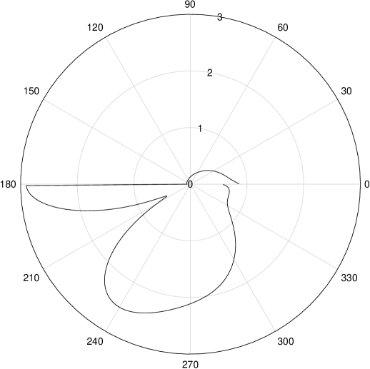
Figure 3: Variation of the function $P(r,\theta)$ for $r=5$ and $0\leq\theta\leq 2\pi$ when $\theta_{0}=\pi/4$, $\rho_{f}/m_{0}=100$, $d=d_{1}=d_{2}=0.01$, $a=0.001$, $|k|=1$, $\arg k=\tan^{-1}0.1$, $|\alpha|=10$.

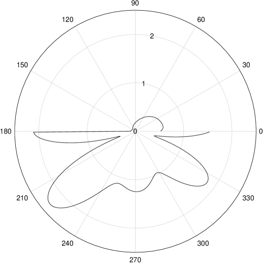
Figure 4: Variation of the function $P(r,\theta)$ for $r=5$ and $0\leq\theta\leq 2\pi$ when $\theta_{0}=\pi/16$, $\rho_{f}/m_{0}=100$, $d=d_{1}=d_{2}=0.01$, $a=0.001$, $|k|=1$, $\arg k=\tan^{-1}0.1$, $|\alpha|=10$.

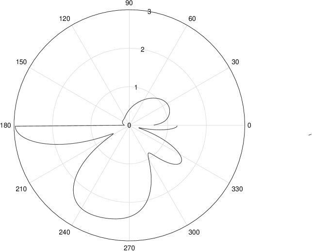
Figure 5: Variation of the function $P(r,\theta)$ for $r=5$ and $0\leq\theta\leq 2\pi$ when $\rho_{f}/m_{0}=500$, $\theta_{0}=\pi/4$, $|\alpha|=10$, $d=d_{1}=d_{2}=0.01$, $a=0.001$, $|k|=1$, $\arg k=\tan^{-1}0.1$, $|\alpha|=10$.

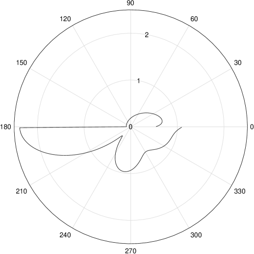
Figure 6: Variation of the function $P(r,\theta)$ for $r=3$ and $0\leq\theta\leq 2\pi$ when $\theta_{0}=\pi/4$, $\rho_{f}/m_{0}=100$, $d=d_{1}=d_{2}=0.01$, $a=0.001$, $|k|=1$, $\arg k=\tan^{-1}0.1$, $|\alpha|=10$.

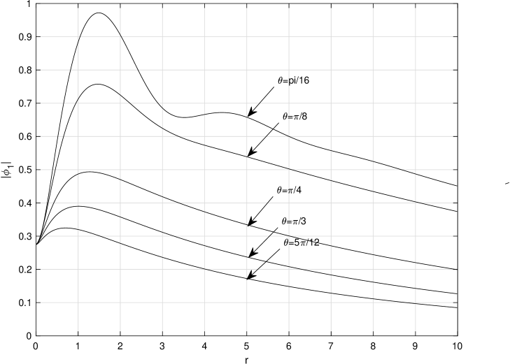
Figure 7: Variation of the function $P(r,\theta)=|\phi_{1}(x,y)|$ versus $r$ for $\theta=\pi/16,\pi/8,\pi/4,\pi/3$, and $5\pi/12$ when $\theta_{0}=\pi/4$, $\rho_{f}/m_{0}=100$, $d=d_{1}=d_{2}=0.01$, $a=0.001$, $|k|=1$, $\arg k=\tan^{-1}0.1$, $|\alpha|=10$.

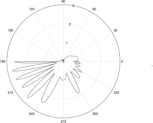
Figure 8: Variation of the function $P(r,\theta)$ for $r=5$ and $0\leq\theta\leq 2\pi$ when $|k|=5$, $\arg k=\tan^{-1}0.02$, $|\alpha|=250$, $\theta_{0}=\pi/4$, $\rho_{f}/m_{0}=100$, $d=d_{1}=d_{2}=0.01$, $a=0.001$.

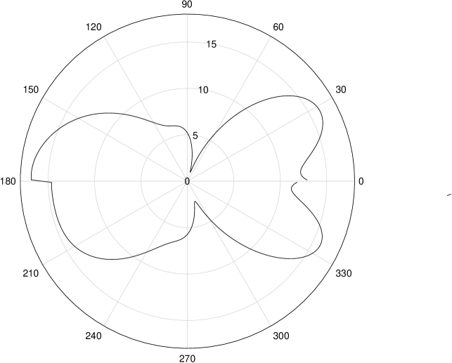
Figure 9: Variation of the function $P(r,\theta)$ when $r=5$, $0\leq\theta\leq 2\pi$ and $k$ is close to the resonance value $k_{res}$. The parameters are $\theta_{0}=\pi/4$, $\rho_{f}/m_{0}=100$, $d=d_{1}=d_{2}=0.2$, $a=0.005$, $|k|=1$, $\arg k=\tan^{-1}0.02$, $|\alpha|=10.$

For our computations, we shall use the solution obtained in Section 3 and consider the case $0<\theta_{0}<\pi/2$. In this case we may choose $\kappa_{0}=0$, and the contour $L$ is the real axis. By inverting the integrals (3.4) and employing formula (3.7) we express the two potential $\phi_{0}(x,y)$ and $\phi_{1}(x,y)$ through the solution of the Riemann-Hilbert problem (3.14) to (3.16)

$$\phi_{0}(x,y)=\frac{1}{2\pi}\int_{-\infty}^{\infty}[\Phi_{0+}(s,0)+\Phi_{0-}(s,0)]e^{\gamma y-isx}ds,\quad y<0.$$

$$\phi_{1}(x,y)=\frac{1}{2\pi}\int_{-\infty}^{\infty}[\Phi_{1+}(s,0)+\Phi_{1-}(s,0)]e^{-\gamma y-isx}ds,\quad y>0.$$ (5.1)

On substituting formulas (3.56) and (3.68) into these expressions we transform them as

$$\phi_{0}(x,y)=C\hat{\Omega}_{0}(r,\theta)+N\hat{\Omega}_{1}(r,\theta)+\hat{\Omega}_{2}(r,\theta),\quad y<0,$$

$$\phi_{1}(x,y)=C\tilde{\Omega}_{0}(r,\theta)+N\tilde{\Omega}_{1}(r,\theta)+\tilde{\Omega}_{2}(r,\theta),\quad y>0,$$ (5.2)

where $(r,\theta)$ are the polar coordinates of a point $(x,y)$, $x=r\cos\theta$, $y=r\sin\theta$,

$$\hat{\Omega}_{0}(r,\theta)=\frac{1}{2\pi}\int_{-\infty}^{\infty}[\Lambda_{1}^{+}(t)-\Lambda_{1}^{-}(t)-\eta_{0}\Lambda_{2}^{+}(t)+\eta_{0}\Lambda_{2}^{-}(t)]\frac{v_{+}(t,r,\theta)dt}{t-\zeta_{0}},$$

$$\hat{\Omega}_{j}(r,\theta)=\frac{1}{2\pi}\int_{-\infty}^{\infty}[\Lambda_{1}^{+}(t)\Psi_{0+}^{(j)}(t)-\Lambda_{1}^{-}(t)\Psi_{0-}^{(j)}(t)-\Lambda_{2}^{+}(t)\Psi_{1+}^{(j)}(t)+\Lambda_{2}^{-}(t)\Psi_{1-}^{(j)}(t)]v_{+}(t,r,\theta)dt,\$$

$$\tilde{\Omega}_{0}(r,\theta)=\frac{1}{2\pi}\int_{-\infty}^{\infty}[\Lambda_{2}^{-}(t)-\Lambda_{2}^{+}(t)-\eta_{0}\Lambda_{0}^{-}(t)+\eta_{0}\Lambda_{0}^{+}(t)]\frac{v_{-}(t,r,\theta)dt}{t-\zeta_{0}},$$

$$\tilde{\Omega}_{j}(r,\theta)=\frac{1}{2\pi}\int_{-\infty}^{\infty}[\Lambda_{2}^{-}(t)\Psi_{0-}^{(j)}(t)-\Lambda_{2}^{+}(t)\Psi_{0+}^{(j)}(t)-\Lambda_{0}^{-}(t)\Psi_{1-}^{(j)}(t)+\Lambda_{0}^{+}(t)\Psi_{1+}^{(j)}(t)]v_{-}(t,r,\theta)dt,$$

$$j=1,2,\quad v_{\pm}(t,r,\theta)=e^{[\pm\gamma(t)\sin\theta-it\cos\theta]r},$$ (5.3)

and the functions $\Lambda_{j}^{\pm}(t)$ are given by (3.69).

The improper integrals over the real axis $L$ are computed by mapping the contour $L$ onto the unit, positively oriented circle ${\cal C}=\{|u|=1\}$ and applying the Simpson rule,

$$\int_{L}S(t)dt=-4\int_{\cal C}\frac{S(t)du}{(u-i)^{2}}=-4i\int_{\pi/2}^{5\pi/2}\frac{S(t)ud\theta}{(u-i)^{2}},$$ (5.4)

where $t=-2i(u+i)(u-i)^{-1}$ and $u=e^{i\theta}$. The principal value of the Cauchy integrals over the contour $L$ are computed by employing the same mapping to the unit circle ${\cal C}$ and the following formula:

$$\frac{1}{2\pi i}\int_{L}\frac{S(t)dt}{t-s}=\frac{\sigma-i}{2\pi i}\int_{\cal C}\frac{S(t)du}{(u-i)(u-\sigma)}$$

$$=\frac{\sigma-i}{2(2n+1)}\sum_{j=-n}^{n}\frac{S(t_{j})}{u_{j}-i}\left[1+\frac{2i\sin((\theta-\theta_{j})n/2)\sin((\theta-\theta_{j})(n+1)/2)}{\sin((\theta-\theta_{j})/2)}\right],\quad s\in L,$$ (5.5)

where

$$\sigma=i\frac{s-2i}{s+2i},\quad\theta=-i\log\sigma,\quad t_{j}=-2i\frac{u_{j}+i}{u_{j}-i},\quad u_{j}=e^{i\theta_{j}},\quad\theta_{j}=\frac{2\pi j}{2n+1},$$ (5.6)

and $n$ is the number of knots of the integration formula. For computing integrals (3.31), (3.43), and (3.45) we apply the Gauss quadrature formula with Chebyshev’s weights and abscissas.

In our numerical tests, we focus our attention on the absolute values of the full potentials $\psi_{0}=\psi_{inc}+\phi_{ref}+\phi_{0}$ in the lower half-plane ${{H}_{0}}$ and $\psi_{1}=\phi_{1}$ in the upper half-plane ${{H}_{1}}$. Denote by $P(r,\theta)=|\psi_{1}(x,y)|$, $(x,y)\in{{H}_{1}}$ ($0<\theta<\pi$) and $P(r,\theta)=|\psi_{0}(x,y)|$, $(x,y)\in{{H}_{0}}$ ($\pi<\theta<2\pi$). For all tests we choose water’s density $\rho_{f}=997$ kg/m³. Except for Figs. 8 and 9, we choose $\arg k=\tan^{-1}0.1$, $|k|=1$ m^-1, the cell measurements $d=d_{1}=d_{2}=0.01$ m, and the aperture radius $a=0.001$ m. In this case the parameter $\tau$ is complex and its magnitude is small, $\tau=5.035610^{-2}+i5.153110^{-3}$.

The curves drawn in Figs 3 to 6 show the variation of the function $P(r,\theta)$ with change of $\theta$ when $r$ is kept constant. In Fig. 3, we use $\theta_{0}=\pi/4$, $|\alpha|=10$ m^-3, $\rho_{f}/m_{0}=100$ m^-1, and $r=5$ m. For Fig. 4, we choose the same parameters as for Fig. 3 except for $\theta_{0}=\frac{\pi}{16}$. In Fig. 5, we increase the ratio $\rho_{f}/m_{0}$ from 100 to 500 that results in a fivefold decrease of the panel surface density. The other parameters coincide with those employed for computations portrayed in Fig. 3. It is possible to infer from this figure that as the membrane surface density increases the absolute value of the potential $\psi_{1}$ is decreases. In Fig. 6, we decrease $r$ and select it to be $3$ m and keep the other parameters of Fig. 3 unchanged. Fig. 7 shows how the function $P(r)$ varies with change of $r$ when the polar angle $\theta$ equals $\pi/16$, $\pi/8$, $\pi/4$, $\pi/3$, and $5\pi/12$, while the other parameters are selected the same way as in Fig. 3. In Fig. 8, we increase the value of $|k|$ from 1 to $5$, change its argument, $\arg k=\tan^{-1}0.02$, and because of formula (2.7), increase $|\alpha|$ from 10 to 250. The other parameters of Fig. 3 are the same.

As $k_{2}\to 0^{+}$ and $k_{1}\to k_{res}=\sqrt{2a/V}$, the parameter $\tau\to\infty$. In Fig. 9, we change the cell measurements, the aperture radius, and $\arg k$, $d=d_{1}=d_{2}=0.2$ m, $a=0.005$ m and $\arg k=\tan^{-1}0.02$, and keep the other parameters the same as in Fig. 3. In this case $\tau=0.96881+i0.17439$. It is seen that when $|\tau|$ is growing, the magnitude of the function $P(r)$ is also growing. We have $P(r)\to\infty$ as the wave number $k$ approaches the resonance value $k_{res}$.

6 Conclusions

A closed-form solution has been given for the model problem of the scattering of a plane sound wave by an infinite thin structure formed by a semi-infinite acoustically hard screen attached to a sandwich panel with acoustically hard walls. The upper side of the sandwich panel is perforated, while the lower side is an unperforated membrane. We have applied two methods of extension of the boundary conditions to the whole real axis and deduce two order-2 vector Riemann-Hilbert problems. The matrix coefficients of both problems have the Chebotarev-Khrapkov structure with the same order-4 characteristic polynomial but with distinct entries. Wiener-Hopf matrix factors for both problems have been derived by quadratures by solving a scalar Riemann-Hilbert problem on the same elliptic surface. The coefficient of the scalar problem is equal to the first eigenvalue of the matrix on the upper sheet of the surface and the second eigenvalue on the lower sheet. We have eliminated the essential singularity caused by simple poles of the Cauchy analogue at the two infinite points of the surface by solving a genus-1 Jacobi inversion problems in terms of the Riemann $\theta$-function.

We have found that the analysis of the Wiener-Hopf matrix factors at infinity is simpler for the first method that sets the Riemann-Hilbert problem for the one-sided Fourier transforms of the velocity potentials on the upper and lower sides of the infinite structure. The second method extends the four boundary conditions to the whole real axis by means of unknown functions and employ the one-sided Fourier transforms of these functions. The advantage of the first method over the second one is explained by the presence of the logarithmic growth at infinity of the densities of the singular integrals involved in the solution obtained by the second method. Both methods lead to the solution having two arbitrary constants. The constants have been fixed by additional conditions of the problem. For the first method, in addition to the meromorphic Wiener-Hopf factors, we constructed the canonical matrix of factorization and computed the partial indices of factorization. It turns out that they both are equal to zero and therefore stable.

Numerical tests have been implemented for the solution derived by the first method. The integrals involved are rapidly convergent for all values of the parameters tested except for the case when $|\tau|\to\infty$, when the method is not numerically efficient. We have computed the absolute values of the full velocity potentials, the function $P(r,\theta)=|\phi_{1}|$, $0<\theta<\pi$, and $P(r,\theta)=|\phi_{inc}+\phi_{ref}+\phi_{0}|$, $\pi<\theta<2\pi$. We have found that the presence of the sandwich panel perforated from the upper side reduces the transmission of sound, and when the membrane surface density $m_{0}$ is growing the function $P(r,\theta)$ ($0<\theta<\pi)$ decreases. We have also discovered that when the absolute value $|k|$ of the complex wave number approaches the resonance value $k_{res}$, then $|\tau|\to\infty$ and the magnitude of the function $P(r,\theta)$ tends to infinity.

References

1. J. E. Ffowcs Williams, The acoustics of turbulence near sound absorbent liners, J. Fluid Mech. 51 (1972) 737-749..

2. F. G. Leppington and H. Levine, Reflexion and transmission at a plane screen with periodically arranged circular or elliptical apertures. J. Fluid Mech. 61 (1973) 109-127.

3. F. G. Leppington, The effective boundary conditions for a perforated elastic sandwich panel in a compressible fluid, Proc. R. Soc. A 427 (1990) 385-399.

4. C. M. A. Jones, Scattering by a semi-infinite sandwich panel perforated on one side, Proc. R. Soc. A 431 (1990) 465-479.

5. Y. A. Antipov and V. V. Silvestrov, Factorization on a Riemann surface in scattering theory, Quart. J. Mech. Appl. Math. 55 (2002) 607-654.

6. N.G.Moiseyev, Factorization of matrix functions of special form, Soviet Math. Dokl. 39 (1989) 264-267.

7. Y. A. Antipov and N. G. Moiseyev, Exact solution of the plane problem for a composite plane with a cut across the boundary between two media, J. Appl. Math. Mech. (PMM) 55 (1991) 531-539.

8. G. N. Chebotarev, On closed-form solution of a Riemann boundary value problem for n pairs of functions, Uchen. Zap. Kazan. Univ. 116 (1956) 31-58.

9. A. A. Khrapkov, Certain cases of the elastic equilibrium of an infinite wedge with a non- symmetric notch at the vertex, subjected to concentrated forces, J. Appl. Math. Mech. (PMM) 35 (1971) 625-637.

10. V. G. Daniele, On the solution of two coupled Wiener–Hopf equations, SIAM J. Appl. Math. 44 (1984) 667-680.

11. I. D. Abrahams, On the non-commutative factorization of Wiener–Hopf kernels of Khrapkov type, Proc. R. Soc. A 454 (1998) 1719-1743.

12. E. I. Zverovich, Boundary value problems in the theory of analytic functions in Hol̈der classes on Riemann surfaces, Russian Math. Surveys 26 (1971) 117-192.

13. A. Krazer, Lehrbuch der Thetafunktionen, Teubner, Leipzig 1903.

14. G. Springer, Introduction to Riemann Surfaces, Addison–Wesley, Reading, MA 1956.

15. I. Papanikolaou and F. G. Leppington, Acoustic scattering by a parallel pair of semi-infinite wave-bearing surfaces, Proc. R. Soc. A 455 (1999) 3743-3765.

16. A. P. Dowling and J. E. Ffowcs Williams, Sound and Sources of Sound, Ellis Horwood, Chichester, 1983.

17. Y.A. Antipov and V.V. Silvestrov, Electromagnetic scattering from an anisotropic half-plane at oblique incidence: the exact solution, Quart. J. Mech. Appl. Math. 59 (2006) 211-251.

18. F. D. Gakhov, Riemann boundary-value problem for a system of n pairs of functions, Russian Math. Surveys 7 (1952) 3-54.

19. N. I. Muskhelishvili, Singular Integral Equations, Noordhoff, Groningen 1958.

20. N. P. Vekua, Systems of Singular Integral Equations Noordhoff, Groningen 1967.

21. I. Gohberg and M. G. Krein, On the stability of a system of partial indices of the Hilbert problem for several unknown functions, Dokl. AN SSSR 119 (1958) 854-857.