Probably Approximately Correct Federated Learning

Abstract

Federated learning (FL) is a distributed learning framework with privacy, utility, and efficiency as its primary concerns. Existing research indicates that it is unlikely to simultaneously achieve privacy protection, utility and efficiency. How to find an optimal trade-off for the three factors is a key consideration for trustworthy federated learning. Is it possible to cast the trade-off as a multi-objective optimization problem in order to minimize the utility loss and efficiency reduction while constraining the privacy leakage? Existing multi-objective optimization frameworks are not suitable for this goal because they are time-consuming and provide no guarantee for the existence of the Pareto frontier for solutions. This challenge motivates us to seek an alternative solution to transform the multi-objective problem into a single-objective problem, which can potentially be more cost-effective and optimal. To this end, we present FedPAC, a unified framework that leverages PAC learning to quantify multiple objectives in terms of sample complexity. This unification provides a quantification that allows us to constrain the solution space of multiple objectives to a shared dimension. We can then solve the problem with the help of a single-objective optimization algorithm. Specifically, we provide the theoretical results and detailed analyses on how to quantify the utility loss, privacy leakage, and efficiency, and show that their trade-off can be attained at the maximal cost on potential attackers from the PAC learning perspective.

Keywords: Federated learning, PAC learning, Multi-objective optimization, Trade-off, Generalization error bounds

1 Introduction

Federated learning (FL) is a trustworthy machine learning framework, where privacy, utility, and efficiency are the three main concerns that must be scrutinized and optimized. Existing research has shown that there always exists a trade-off among privacy protection, utility and efficiency (Zhang et al. (2019)). How to find an optimal trade-off among all desired objectives is a key consideration when designing and deploying the FL framework in practice (Tsipras et al. (2018)).

Most of the existing works cast the above-mentioned trade-off problem as a constrained optimization problem, which aims to minimize certain objectives subject to imposed constraints. For example, (Makhdoumi and Fawaz, 2013; du Pin Calmon and Fawaz, 2012) formulated the privacy-utility trade-off as an optimization problem where private information leaked to the adversary is minimized subject to a given set of utility constraints. (Rassouli and Gündüz, 2019) illustrated that the optimal privacy-utility trade-off can be solved using a standard linear program and provided a closed-form solution for the special case when the data to be released is a binary variable. In essence, this line of research can be generalized to the following multi-objective constrained optimization problem:

$$\begin{array}[]{r@{\quad}l@{}l@{\quad}l}\quad\min&(\epsilon_{1},\ \dots,\ \epsilon_{k})\\ \text{subject to}&\epsilon_{k+j}\leq\alpha_{j},\ \ \ \ \forall\ j\in\{1,\cdots,m\},\end{array}$$ (3)

In the above, $(\epsilon_{1},...,\epsilon_{k})$ denote objectives to be optimized in federated learning and $(\epsilon_{k+1},...,\epsilon_{k+m})$ are constrains to be fulfilled. The constrained multi-objective optimization as such poses several challenges that do not admit trivial solutions. First, one must prescribe in advance a proper constraint (i.e., $\alpha_{j}$) that ensures feasible solutions of equation 3 to be useful in practice. Unfortunately, existing multi-objective optimization frameworks do not guarantee the existence of Pareto solutions that minimizes all objective functions simultaneously (Miettinen (1999); Hassanzadeh and Rouhani (2010)); Second, in most cases, the objective function of equation 3 is usually not convex, direct multi-objective optimization cannot make use of efficient gradient-based approaches, and are often time-consuming by using e.g. evolution-based methods ( Tian et al. (2022b, a); Cheng et al. (2022); Liu et al. (2022); Hua et al. (2021)); Third, the problem of equation 3 can be scalarized into the single objective optimization problem (i.e., $\lambda_{1}\epsilon_{1}+\dots+\lambda_{k}\epsilon_{k}$), yet it remains an open problem of how to set proper scalarizing coefficients such that optimal solutions can reach every Pareto optimal solutions of the original problem. Furthermore, when considering how to model the efforts of potential attackers in the FL framework, we need to unify both the protection and the attacking mechanisms. If we can find a unifying dimension in which to compare these efforts, it would be much easier to optimize the trustworthy FL framework under all three objectives.

Taking consideration of the aforementioned challenges of multi-objective problems, we propose a new unified framework that leverages the PAC learning theory (Valiant (1984)) to quantify multiple objectives in terms of the sample complexity (denoted as $s$). The sample complexity is used in the PAC learning framework to measure the number of samples needed for a learning model to attain a certain level of competence within a given confidence level. This number can be used to measure both the costs for the defender and the attacker in an FL framework. With this in mind, we can reformulate the optimal trade-off problem as equation 6.

$$\begin{array}[]{r@{\quad}l@{}l@{\quad}l}\quad\mathop{\min}\limits_{s}&f(\epsilon_{1}(s),\epsilon_{2}(s),\dots,\epsilon_{k}(s))\\ \text{subject to}&\epsilon_{i}\leq f_{i}(s),\ \ \ \ \ \ \ \forall\ i\in\{1,\dots,k,\dots,(k+m)\}.\end{array}$$ (6)

Here, $f$ is a specific function with sample complexity ($s$) as its variables. We list the advantages of equation 6 as follows:

1. Solutions for multiple objectives of equation 6 share the same space (i.e., sample complexity), while the solution spaces of equation 3 are independent of each other. A shared and small dimensional space means that it is more likely to achieve the optimal solution instead of a suboptimal one.

2. Following up the aforementioned conclusion, theoretically, it can potentially be more efficient to find the optimal solution in a smaller search space.

3. Sample complexity is easier to understand and applied to model both the attackers’ costs and protection expenses, thus leading to a trade-off mechanism for both the attackers and the defenders.

The main contributions of our paper are summarized as follows:

• We present a unified framework to analyze the federated learning algorithm. Specifically, we proposed FedPAC framework, to measure and quantify privacy leakage (Definition 4.1), utility loss (Definition 5.1), and training efficiency (Definition 5.2).

• From the PAC learning perspective, we provide the upper bound for the utility loss (Theorem 5.1) and privacy leakage (Theorem 4.1), and further formalize the privacy-utility-efficiency trade-off expression (Theorem 5.3). Based on these results, we formalize the concept of private PAC learning (Corollary 1), which serves as the basis for the algorithmic proposal of a novel protection mechanism.

• For the attacker, we provide a detailed analysis about the upper bound of the privacy leakage (Section 4.1), and analyze the cost of the attacker from the perspective of PAC learning (Section 4.2).

• For the protector, we provide a detailed analysis about the upper bound of the utility loss (Section 5.1). Specifically, we analyze the utility loss caused by different protection mechanisms separately, including Randomization (Geyer et al. (2017); Truex et al. (2020); Abadi et al. (2016)) and Homomorphic Encryption (HE) (Gentry and Boneh (2009); Zhang et al. (2020a)) (Section 5.3).

Our paper is organized as follows: In section 2, we first provide necessary preliminary to better understand this paper, including learning scenario setting in section 2.1, threat model in section 2.2, and summarize our main results in section 2.3. In section 3, we review some related works of our paper, including privacy-utility-efficiency trade-off, multi-objective optimization, and PAC learning; In section 4, we focus on the attacker, we provide a detailed analysis of the upper bound of privacy leakage and the cost of the attacker. In section 5, we focus on the protector and provide a detailed analysis of the upper bound of utility loss in the presence of different protection mechanisms. In section 6, we discuss how our results provide theoretical bounds on the gains and losses of privacy, utility, and efficiency in federated learning.

2 Preliminary

In this section, we describe the learning scenario setting and threat model of our paper, as well as briefly summarize the main results.

2.1 Learning scenario setting

In this work, we consider the learning scenario based on horizontal federated learning (HFL), as shown in Figure 1.

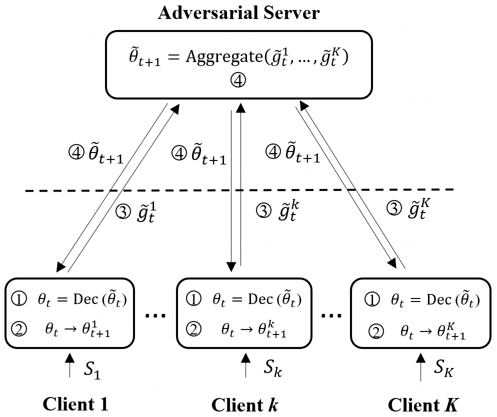
Figure 1: Learning scenario of our work.

We assume there are a total of $K$ clients collaboratively to learn a shared model, the server side is an adversary attacker, and each client acts as a protector to prevent privacy leakage. For convenience, we first provide the notation used throughout this article, as shown in table 1.

We follow the FL training procedure of federated averaging (FedAvg) (McMahan et al. (2017)), plus adding protection mechanisms for the sake of security concerns. Without loss of generality, suppose the training process is running on the $t$-th round iteration, let $\theta_{t}$ be the aggregated global model at round $t$, $\eta_{t}$ represent the learning rate, and $\delta_{t}^{(k)}$ be the distortion applied to protect the local information of client $k$ at iteration $t$. We denote $\mathcal{D}_{\text{\rm prot}}^{(k)}=\{\textbf{X}^{(k)},\textbf{Y}^{(k)}\}=\{(X_{1}^{(k)},Y_{1}^{(k)}),\cdots,(X_{m_{k}}^{(k)},Y_{m_{k}}^{(k)})\}$ as the local training set of client $k$, and $\mathcal{L}$ represents the loss function. The training process for privacy-preserving HFL contains the following four steps:

• Upon receiving the global model $\widetilde{\theta}_{t}$ at round $t$, each protector decodes the global model $\theta_{t}\leftarrow\text{Dec}(\widetilde{\theta}_{t})$.

  Please note that, some protection mechanisms, e.g., Randomization (Geyer et al. (2017); Truex et al. (2020); Abadi et al. (2016)), do not have the decoding procedure. However, for consistency, we keep this step and set $\text{Dec}(\widetilde{\theta}_{t})=\widetilde{\theta}_{t}$ for those who without decoding operation.

• Take client $k$ as an example, with the decoded global model, the protector $k$ updates its local model parameters using SGD as:

  $$\theta_{t+1}^{(k)}\leftarrow\theta_{t}-\eta_{t}\cdot\frac{1}{|\mathcal{D}_{\text{\rm prot}}^{(k)}|}\sum_{i=1}^{|\mathcal{D}_{\text{\rm prot}}^{(k)}|}\nabla\mathcal{L}(\theta_{t},X_{i}^{(k)},Y_{i}^{(k)})$$ (7)

• The protector $k$ uploads the distorted gradient to the server, which is defined as:

  $$\widetilde{g}_{t}^{(k)}\leftarrow\frac{1}{|\mathcal{D}_{\text{\rm prot}}^{(k)}|}\sum_{i=1}^{|\mathcal{D}_{\text{\rm prot}}^{(k)}|}\nabla\mathcal{L}(\theta_{t},X_{i}^{(k)},Y_{i}^{(k)})+\delta_{t}^{(k)},$$ (8)

  where $\delta_{t}^{(k)}$ represents the distortion added by client $k$ at round $t$;

• Upon receiving distorted gradients from all clients, the server aggregates these information and updates global model as:

  $$\widetilde{\theta}_{t+1}\leftarrow\widetilde{\theta}_{t}-\eta_{t}\cdot\sum_{k=1}^{K}\frac{|\mathcal{D}_{\text{\rm prot}}^{(k)}|}{\sum_{k=1}^{K}|\mathcal{D}_{\text{\rm prot}}^{(k)}|}\widetilde{g}_{t}^{(k)}$$ (9)

  After that, the server dispatches $\widetilde{\theta}_{t+1}$ to all clients and follows the above steps for the next round.

2.2 Threat model

We consider the server is a semi-honest attacker, he/she follows the FL protocol, yet may execute privacy attacks on exposed data to deduce the private information of other participants, e.g., gradient inversion attacks proposed by Zhu et al. (2019). Specifically, the attacker has two main tasks, as shown in Figure 2.

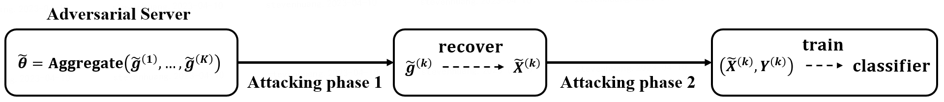
Figure 2: Threat Model.

• Attacking Phase 1: Out of curiosity, the attacker takes the distorted gradient $\widetilde{g}^{(k)}$ of client $k$, and utilizes different attack approaches to recover the dataset (denoted as $\widetilde{X}^{(k)}$). The goal is to restore the original dataset as much as possible.

• Attacking Phase 2: The attacker wants to know and quantify the cost of the attack approach, so they simulate an experiment for this purpose. Specifically, they utilized the recovered dataset ( $\widetilde{X}^{(k)}$), with their corresponding true label $Y^{(k)}$ to train a classifier. The goal is to deduce how many samples are needed to make the classifier satisfies $(\epsilon,\delta)$-PAC learnability.

2.3 Main Results

Under the aforementioned setting, our goal is to build a unified framework in which privacy, utility, and efficiency can be measured from the PAC learning perspective. Based on that, we further formalize the key conclusion of this paper: How to quantify the trade-off between privacy, utility, and efficiency from the perspective of PAC learning ? To better understand the workflow of our main results, we illustrate the roadmap in Figure 3 for convenience.

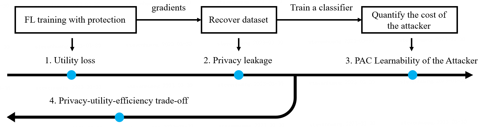
Figure 3: Roadmap of our main results.

1. The FL system follows the training procedure described in section 2.1 to execute FL training. Because protection mechanisms are utilized to protect the information, which might potentially lead to the utility loss.

2. Following Phase 1 described in section 2.2, whenever the server side (attacker) receives the distorted gradients from clients, the attacker trys to recover the dataset, and inevitably leads to the privacy leakage.

3. Following Phase 2 described in section 2.2, the attacker further wants to evaluate the cost of the attack approach, so as to decide whether to launch an attack.

4. Based on privacy leakage and utility loss, we expect to formalize the privacy-utility-efficiency trade-off.

Specifically, we will discuss the following questions and provide the results, as well as detailed analyses correspondingly (see Figure 4 for the illustration).

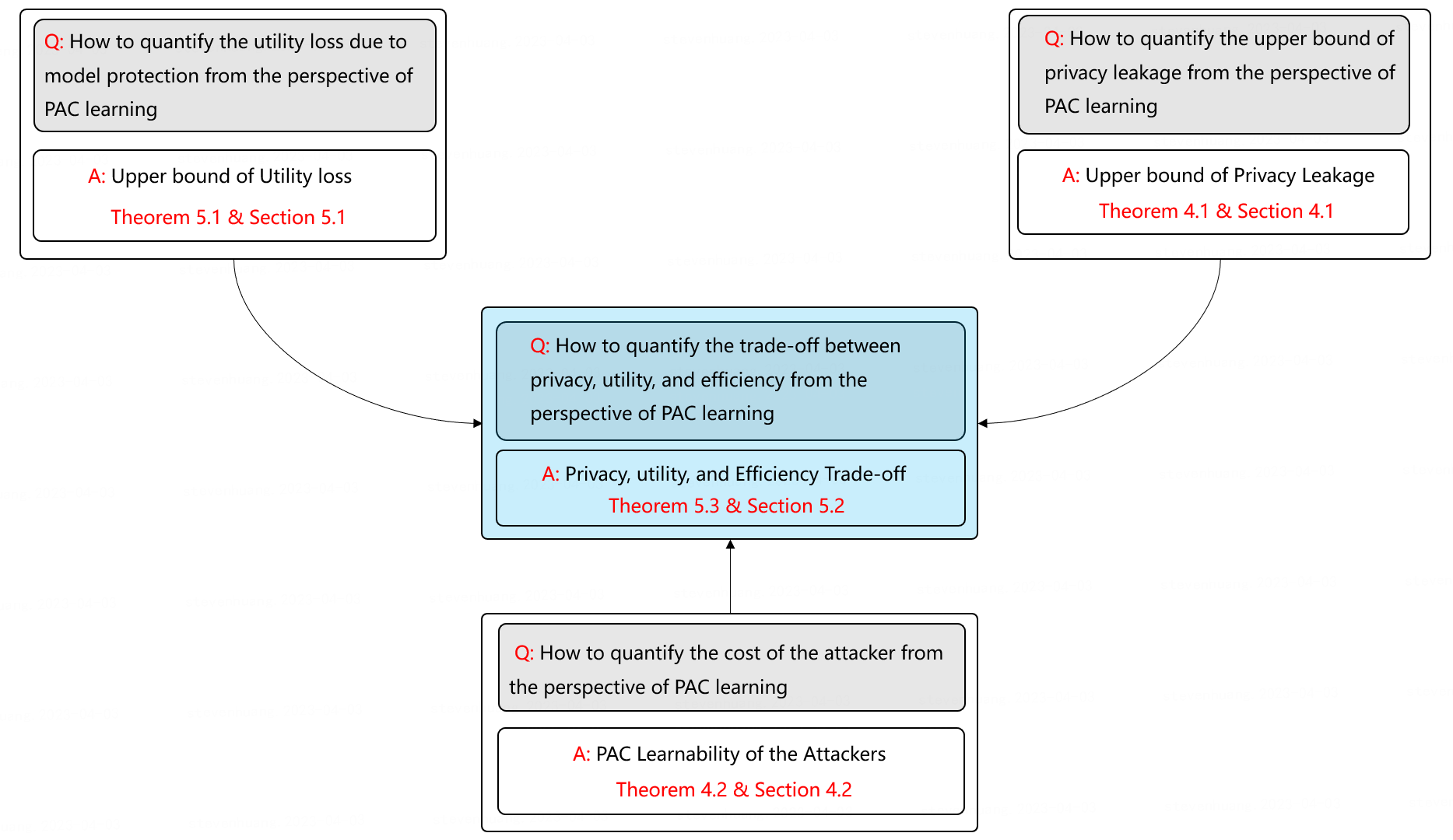
Figure 4: Illustration of our main results.

1. Q: How to quantify the upper bound of privacy leakage (Definition 4.1) from the perspective of PAC learning?

   A: Privacy leakage measures the gap between the recovered dataset by the attacker and the original dataset. We argue that the upper bound of privacy leakage relies on the size of the training samples. Intuitively, the more training samples, the smaller the upper bound of the privacy leakage of the model, which means that, With the same probability, it is more challenging to attack the model.

   Please refer to Theorem 4.1 for formal definition, and we provide detailed analyses in Section 4.1.

2. Q: How to quantify the cost of the attacker from the perspective of PAC learning?

   A: To quantify the cost of the attack approach, we simulate an experiment to train a classifier with the recovered dataset, we provide the lower bound of sample sizes for this purpose, which means how many samples are needed to make the classifier satisfy $(\epsilon,\delta)$-PAC learnability.

   Please refer to Theorem 4.2 for formal definition, and we provide detailed analyses in Section 4.2.

3. Q: How to quantify the utility loss (Definition 5.1) due to model protection from the perspective of PAC learning?

   A: Utility loss measures the gap between the performance of the model before and after adding protection. We argue that the upper bound of utility loss relies on the size of the training samples. Intuitively, the more training samples, the smaller the upper bound of the utility loss of the model, which means that the model can achieve better model performance with the same probability.

   Please refer to Theorem 5.1 for formal definition, and we provide detailed analyses in Section 5.1.

4. Q: How to quantify the trade-off between privacy, utility, and efficiency from the perspective of PAC learning?

   A: Combining the upper bound of utility loss and the upper bound of privacy leakage, by sample complexity, we can unify these three dimensions and establish the trade-off expression between utility, privacy and efficiency.

   Please refer to Theorem 5.3 for formal definition, and we provide detailed analyses in Section 5.2.

3 Related Work

The concept of Federated Learning was first proposed in 2016 (McMahan et al. (2017); Yang et al. (2019a)). There are many surveys and books that cover all aspects of federated learning research (Yang et al. (2023); Kairouz et al. (2021); Li et al. (2020); Yang et al. (2019b)). In summary, existing research can be categorized into three folds, i.e., privacy, utility, and efficiency. However, most of the research is interest in addressing each of these challenges separately, while there is relatively less focus on how to make trade-offs between these three dimensions.

In this section, we provide an overview of the trade-off problem, multi-objective optimization, and also review the basic knowledge of PAC learning, as well as how PAC learning can be applied to theoretical analysis of machine learning algorithms.

3.1 Privacy-utility-efficiency trade-off

The privacy-utility trade-off problem has been extensively studied in many areas, such as machine learning, database queries, etc. A well-known theory in this area is differential privacy (DP), where the goal is to prevent information leakage by adding an amount of randomness (Dwork (2006)). However, the original DP definition can be overly cautious by focusing on worst-case scenarios, following this work, more flexible and generalized versions have been proposed to remedy this shortcoming, such as $(\epsilon,\delta)$-differential privacy, Rényi differential privacy (Mironov (2017)), etc.

In addition to DP theory, Another research line is to cast the trade-off problem as an optimization problem. Makhdoumi and Fawaz (2013) cast the privacy-utility trade-off as a convex optimization problem, where privacy leakage is modeled under the log-loss by the mutual information between private data and released data, and utility constraint is regarded as the average distortion between original and distorted data. Sankar et al. (2013) utilized rate-distortion theory to develop privacy-utility trade-off region for i.i.d. data sources with known distribution. Chen et al. (2020) develop novel encoding and decoding mechanisms that simultaneously achieve optimal privacy and communication efficiency in various canonical settings under distributed learning scenarios. Zhong and Bu (2022) investigates the privacy-utility trade-off problem for seven popular privacy measures in two different scenarios: global and local privacy.

Under FL scenarios, many algorithms take into account the balance of privacy, utility and efficiency. For example, Zhang et al. (2020b) present BatchCrypt that substantially reduces the encryption and communication overhead caused by HE. Huang et al. (2020) introduce RPN to keep the model performance without loss while reducing the communication overhead. However, such researches are case by case and have no unified theoretical analysis. To fill this gap, Zhang et al. (2022b) proposed No-Free-Lunch (NFL) theorem with a similar motivation to this paper, where privacy, utility, and efficiency are measured by distortion extent, a metric to measure the data distribution difference before and after data protection. However, in most cases, the distortion extent can only be used in the protection mechanisms, which makes it not suitable for analyzing attack algorithms. Besides, the distortion extent is determined by the data distribution, which is usually unknown in advance in real-world applications.

3.2 Multi-objective Optimization

Multi-objective optimization (MOO), also known as Pareto optimization (Miettinen (1999); Hwang and Masud (2012); Hassanzadeh and Rouhani (2010)), is an area of mathematical optimization problems involving more than one objective function to be optimized simultaneously. MOO has been widely studied, and most MOO solutions can fall into either one of the following two classes:

• Priori methods (Hwang and Masud (2012)), which require sufficient preference information before the solution process, including lexicographic optimization (Sherali and Soyster (1983); Isermann (1982); Ogryczak et al. (2005); Cococcioni et al. (2018)), Scalarizing (Srinivas and Deb (1994); Miettinen (1998); Wierzbicki (1982); Sen (1983); Golovin and Zhang (2020)), goal programming (Charnes et al. (1955); Tamiz et al. (1998); Jones et al. (2010); Tafakkori et al. (2022)), etc.

• Posteriori methods, which aim at producing all the Pareto optimal solutions, including mathematical optimization (Jeter (1986); Martins and Ning (2021)), evolutionary algorithms (Deb et al. (2002); Deb and Jain (2013); Jain and Deb (2013); Kim et al. (2004); Suman and Kumar (2006); Vargas et al. (2015); Lehman and Stanley (2011)), deep learning-based algorithms (Navon et al. (2020); Liu et al. (2021)), etc.

FL is a new application area for MOO. Xu et al. (2021b) proposes a federated data-driven evolutionary optimization framework that is able to perform data-driven optimization when the data is distributed on multiple devices. Xu et al. (2021a) extends this work and focuses on MOO; Some other research works utilize the MOO to deal with the trade-off among utility, efficiency, robustness, and privacy under FL setting, Liu and Jin (2021) proposes MORAS, a multi-objective robust architecture search algorithm to balance both accuracy and robustness in the presence of multiple adversarial attacks. Yin et al. (2022) applies multi-objective optimization to federated split learning, the goal is to obtain the trade-off solution between the training time and energy consumption. Zhu and Jin (2019) aims to optimize the structure of the neural network models in FL using a multi-objective evolutionary algorithm to simultaneously minimize efficiency and utility. Morell et al. (2022) optimizes communication overhead in FL by modeling it as a multi-objective problem and applying NSGA-II (Deb et al. (2002)) to solve it.

3.3 Probably Approximately Correct learning

Probably Approximately Correct (PAC) learning was first proposed in 1984 by Leslie Valiant (Valiant (1984)). Briefly, PAC learning is a framework for the mathematical analysis of machine learning, under which the learner selects a hypothesis function. The goal is that, with high probability, the selected function will have low generalization error.

PAC learning has been extensively studied and applied to machine learning algorithm analysis. For example, Zhang and Tao (2010) present the risk bounds for Levy processes without Gaussian components in the PAC-learning framework. Balcan et al. (2012) consider the problem of PAC-learning from distributed data and analyze fundamental communication complexity questions involve, as well as provide general upper and lower bounds on the amount of communication needed to learn well. Feldman (2009) studied the properties of the agnostic learning framework, which is a natural generalization of PAC learning. Cullina et al. (2018) extend the PAC learning framework to account for the presence of an adversary, and seek to understand the limits of what can be learned in the presence of an evasion adversary.

There are also some studies that apply PAC learning to distributed learning scenarios. Blum et al. (2017) consider a collaborative learning scenario, in which k players attempt to learn the same underlying concept, they present lower bounds and upper bounds on the sample complexity of collaborative PAC learning. However, they only consider realizable setting. Further, Nguyen and Zakynthinou (2018) extend the results to the realizable and non-realizable settings. Blum et al. (2021) analyzed how the sample complexity of federated learning may be affected by the agents’ desire to keep their individual sample complexities low in the PAC learning setting.

4 On the Learnability of the Attacker

We formulate two phases of learning process for the semi-honest attackers (see Figure 2). During Learning Phase 1, the attacker infers the dataset of the protector upon observing the released model information. During Learning Phase 2, with the inferred dataset, the attacker trains a classifier. To provide a unified analysis framework for trade-off between utility, privacy and efficiency for protection mechanisms including Randomization Mechanism and Homomorphic Encryption Mechanism, we introduce the following two distortion extents during the training process of federated learning, called two-way distortion extent and uplink distortion extent (see Definition 4.3 and Definition 5.3).

4.1 Upper Bound for Privacy Leakage

In this section, we provide theoretical analysis for Learning Phase 1. To illustrate the Learning Phase 1 of the attacker, we elaborate on the goal of the attacker, the evaluation metric of the learning separately. Let $\widetilde{g}^{(k)}$ represent the distorted gradient, and $g^{(k)}$ represent the true gradient of client $k$. We denote $\mathcal{D}_{\text{\rm prot}}^{(k)}=\{\textbf{X}^{(k)},\textbf{Y}^{(k)}\}=\{(X_{1}^{(k)},Y_{1}^{(k)}),\cdots,(X_{m_{k}}^{(k)},Y_{m_{k}}^{(k)})\}$ as the dataset of client $k$. Assume the server is a semi-honest attacker, and is aware of the label information $\{Y_{1}^{(k)},\cdots,Y_{m_{k}}^{(k)}\}$.

Learning Phase $1$ of the Attacker

• With the private dataset $\mathcal{D}_{\text{\rm prot}}^{(k)}$ sampled from the dataset of protector $k$, the protector generates the true gradient $g^{(k)}=\frac{1}{|\mathcal{D}_{\text{\rm prot}}^{(k)}|}\sum_{i=1}^{|\mathcal{D}_{\text{\rm prot}}^{(k)}|}\nabla\mathcal{L}(\theta,X_{i}^{(k)},Y_{i}^{(k)})$;

• To protect the private information, protector $k$ uploads the distorted gradient $\widetilde{g}^{(k)}$ to the server;

• Upon observing the distorted information $\widetilde{g}^{(k)}$, the semi-honest attacker infers the private information.

The recovered dataset of the attacker is denoted as $\mathcal{D}_{\text{\rm attack}}^{(k)}=\{(\widetilde{X}_{1}^{(k)},Y_{1}^{(k)}),\cdots,(\widetilde{X}_{m_{k}}^{(k)},Y_{m_{k}}^{(k)})\}$, and $|\mathcal{D}_{\text{\rm attack}}^{(k)}|=|D_{\text{\rm prot}}^{(k)}|$. Let $X_{t,i}^{(k)}$ represent the $i$-th data recovered by the attacker at the $t$-th round of the optimization algorithm, and $X_{i}^{(k)}$ represent the $i$-th original data. For Phase 1, the goal of the attacker is to minimize the gap between the estimated data and the true data, i.e.,

$$\frac{1}{|\mathcal{D}_{\text{\rm attack}}^{(k)}|}\sum_{i=1}^{|\mathcal{D}_{\text{\rm attack}}^{(k)}|}\frac{1}{T}\sum_{t=1}^{T}\frac{||X_{t,i}^{(k)}-X_{i}^{(k)}||}{D}.$$ (10)

For semi-honest attackers, the privacy leakage is measured using the gap between the estimated dataset and the original dataset.

Definition 4.1 (Privacy Leakage)

Let $X_{t,i}^{(k)}$ represent the $i$-th data recovered by the attacker at the $t$-th round of the optimization algorithm, and $X_{i}^{(k)}$ represent the $i$-th original data. The privacy leakage is measured using

$$\epsilon_{p}^{(k)}=1-\mathbb{E}\left[\frac{1}{|\mathcal{D}_{\text{\rm attack}}^{(k)}|}\sum_{i=1}^{|\mathcal{D}_{\text{\rm attack}}^{(k)}|}\frac{1}{T}\sum_{t=1}^{T}\frac{||X_{t,i}^{(k)}-X_{i}^{(k)}||}{D}\right],$$ (11)

where the expectation is taken with respect to the randomness of the mini-batch $\mathcal{D}_{\text{\rm attack}}^{(k)}$.
Remark: We assume that $||X_{t,i}^{(k)}-X_{i}^{(k)}||\leq D$. Therefore, $\epsilon_{p}^{(k)}\in[0,1]$.

Definition 4.2 (Distorted Feature and Distorted Information)

Let $\mathcal{L}$ be the loss function, and $Y$ be the feature information. We denote $\widetilde{g}$ as the distorted information, and ${\widetilde{X}}$ as the distorted feature satisfying that $\nabla\mathcal{L}(\theta,\widetilde{X},Y)=\widetilde{g}$.

Now we introduce an important measurements related to privacy leakage called the uplink distortion extent.

Definition 4.3 (Uplink Distortion Extent)

The process of sending updated parameter from clients to the server is referred to as uplink. We denote $\theta^{(k)}$ as the original information of client $k$, and $\widetilde{\theta}^{(k)}$ as the distorted information uploaded from client $k$ to the server. The uplink distortion extent of client $k$ is $\Delta_{\text{up}}^{(k)}=\|\theta^{(k)}-\widetilde{\theta}^{(k)}\|$, which measures the gap between the original information and the distorted information, it is related to the amount of privacy leakage and is referred to as the uplink distortion extent.

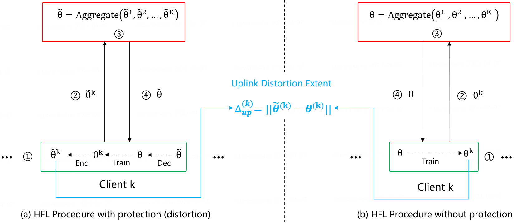
Figure 5: Illustration of uplink distortion extent. The left side is HFL training procedure with protection, and the right side is HFL training procedure without protection.

Assumption 4.1

Assume that $||X_{1}-X_{2}||\leq D$ for any two data. Assume that $c_{a}||\nabla\mathcal{L}(\theta,X_{1},Y)-\nabla\mathcal{L}(\theta,X_{2},Y)||\leq||X_{1}-X_{2}||\leq c_{b}||\nabla\mathcal{L}(\theta,X_{1},Y)-\nabla\mathcal{L}(\theta,X_{2},Y)||$.

Let $d$ represent the dimension of the parameter, and $T$ represent the total number of rounds. The optimization algorithms that guarantee asymptotically optimal regret are all applicable for our analysis, the examples include:

• AdaGrad algorithm proposed by Duchi et al. (2011), achieves an optimal $\Theta(\sqrt{T})$ regret bound. Specifically, the regret bound is $O(\max\{\log d,d^{1-\alpha/2}\sqrt{T}\})$, where $\alpha\in(1,2)$.

• Adam algorithm introduced by Kingma and Ba (2014), achieves an optimal $\Theta(\sqrt{T})$ regret bound. Specifically, the regret bound is $O(\log d\sqrt{T})$ with an improved constant.

The two motivating examples lead to the following assumption.

Assumption 4.2 (Upper and Lower Bounds for Optimization Algorithms)

Let $T$ represent the total number of the learning rounds of the semi-honest attacker. Suppose that $c_{0}\cdot T^{1/2}\leq\sum_{t=1}^{T}||\nabla\mathcal{L}(\theta,X_{t},Y_{t})-\nabla\mathcal{L}(\theta,\widetilde{X}_{t},Y_{t})||=\Theta(T^{1/2})\leq c_{2}\cdot T^{1/2}$, where $X_{t}$ represents the dataset reconstructed by the attacker at round $t$, and ${\widetilde{X}}$ represents the dataset satisfying that $\nabla\mathcal{L}(\theta,\widetilde{X},Y)=\widetilde{g}$.

The reconstruction attack merits in-depth research (Geng et al. (2021)). However, there is a basic lack of theoretical knowledge regarding how and when gradients can result in the unique recovery of original data (Zhu and Blaschko (2020)). The following theorem illustrates a quantitative relationship between privacy leakage $\epsilon_{p}^{(k)}$, the size of the training set $|\mathcal{D}_{\text{\rm prot}}^{(k)}|$ and the uplink distortion extent $\Delta_{\text{up}}^{(k)}$. See Appendix B for more detailed analysis and proof.

Theorem 4.1 (Upper Bound for Privacy Leakage)

Let $T$ represent the total number of the learning rounds of the semi-honest attacker. Let Assumption 4.1 and Assumption 4.2 hold. Assume that $\Delta_{\text{up}}^{(k)}\geq\frac{2c_{2}\cdot c_{b}}{c_{a}\sqrt{T}}$, where $c_{a},c_{2}$ and $c_{b}$ are introduced in Assumption 4.1 and Assumption 4.2. With probability at least $1-\gamma^{(k)}$,

$$\epsilon_{p}^{(k)}\leq 1+\sqrt{\frac{\ln(2/\gamma^{(k)})}{2|\mathcal{D}_{\text{\rm prot}}^{(k)}|}}-\frac{c_{a}}{2D}\cdot\Delta_{\text{up}}^{(k)}.$$ (12)

4.2 PAC Sample Complexity Lower Bound of the Attacker

In this section, we focus on Learning Phase 2 of the attacker, and analyze PAC learnability for the semi-honest attackers. We measure privacy using the distance between the inferred data and the private data, which is referred to as data privacy. Aside from the physical distance, the utility of the inferred data is also a crucial component. To evaluate the utility, we propose Learning Phase 2 for the attacker.

We are curious about the least amount of samples required for the attacker to achieve an error of $\epsilon$ with probability at least $1-\delta$. We provide a lower bound for the number of samples for achieving PAC learnability in terms of the amount of distortion, and show that an exponential amount of samples is necessary to achieve PAC learnability.

Learning Phase $2$ of the Attacker

We denote the dataset of client $k$ recovered by the attacker as ${\mathcal{D}_{\text{\rm attack}}^{(k)}}=\{(\widetilde{X}_{1}^{(k)},Y_{1}^{(k)}),\cdots,(\widetilde{X}_{m_{k}}^{(k)},Y_{m_{k}}^{(k)})\}$, and $|\mathcal{D}_{\text{\rm attack}}^{(k)}|=|\mathcal{D}_{\text{\rm prot}}^{(k)}|$.

Let $h\in\mathcal{H}$ represent the classifier of the learner, and $c$ represent the true classifier.

• The inferred dataset of the attacker is denoted as ${\mathcal{D}_{\text{\rm attack}}^{(k)}}=\{(\widetilde{X}_{1}^{(k)},Y_{1}^{(k)}),\cdots,(\widetilde{X}_{m_{k}}^{(k)},Y_{m_{k}}^{(k)})\}$;

• With the inferred dataset ${\mathcal{D}_{\text{\rm attack}}^{(k)}}$, the attacker trains a classifier $h\in\mathcal{H}$;

• Sample a true labeled example $(X_{\text{\rm test}},c(X_{\text{\rm test}}))$.

The learning problem of the attacker is specified as $\mathcal{F}=(\mathcal{X},\mathcal{Y},\mathcal{C},\mathcal{P},\mathcal{H})$, where $\mathcal{X}$ represents the instance set, $\mathcal{Y}$ represents the label set, $\mathcal{C}$ represents the concept class, and $\mathcal{H}$ represents the hypothesis class. Let $\mathcal{P}$ represent a class of distributions over instances $\mathcal{X}$. Let the probability space be $(\mathcal{X},P,d)$, where $P\in\mathcal{P}$ represents a distribution, and $d$ represents a metric for measuring the distance. Let $c\in\mathcal{C}$ represent the true classifier. The goal of the attacker is to train a classifier based on the inferred dataset, and minimize the risk of the classifier on the true dataset. The question we are concerned about is: when is it possible for the attacker to achieve the $(\epsilon,\delta)$-PAC learning? $(\epsilon,\delta)$-PAC learnability requires the error of the classifier $h$ is at most $\epsilon$ on the original dataset under bounded distortion of the model parameter, with probability at least $1-\delta$.

Risk of the Attacker

The risk of the attacker is taken with respect to the distribution $\widetilde{P}$ and evaluated on the inferred dataset $\widetilde{\mathcal{D}}$,

$$\text{\rm Risk}(h,c)=\Pr_{\widetilde{X}\sim\widetilde{P}}[h(\widetilde{X})\neq c(\widetilde{X})].$$ (13)

Risk depicts the classification loss with the true information, and we also need a quantity that measures the classification loss with the distorted information. The attacker could perturb the victim’s training data but does not know the model initialization, training routine, or architecture of the victim. The victim trains a new model with the poisoned dataset. The performance of the attacker is evaluated according to the accuracy of the victim model on the original (uncorrupted) dataset (Diochnos et al. (2019); Fowl et al. (2021)).

Adversarial Risk of the Attacker

The adversarial risk of the attacker is defined as

$$\text{\rm AdvRisk}(h,c,\Delta)=\Pr_{\widetilde{X}\sim\widetilde{P}}[\exists X\in\mathcal{X}:d(X,\widetilde{X})\leq\Delta,h(X)\neq c(X)],$$ (14)

where the budget $\Delta$ measures the amount of distortion that the protector could introduce considering the constraint on the utility loss. The limitation is measured using some metric $d$ defined over the input space $\mathcal{X}$ and a budget $\Delta$ on the amount of perturbations that the protector can introduce.

The Goals of the Attacker and the Protector

The goal of the attacker is to learn a robust $h$ to minimize the adversarial risk from the inferred dataset. The goal of the protector is to increase the adversarial risk of the attacker, with a small amount of distortion on the transmitted model parameter. The protector aims at finding the label of the original untampered point $X$ by only having its corrupted version $\widetilde{X}$. Therefore, the success criterion of the protector is to reach

$$d(X,\widetilde{X})\leq\Delta,h(X)\neq c(X).$$

Assumption 4.3

For all $1\geq\epsilon\geq 2^{-\Theta(d)}$, there exist two classifiers $c_{1},c_{2}$ (from $\mathcal{X}$ to $\mathcal{Y}$) satisfying that $\Pr_{\widetilde{X}\sim P}[c_{1}(\widetilde{X})\neq c_{2}(\widetilde{X})]=\Theta(\epsilon)$, where $P$ represents a distribution over $\mathcal{X}$.

Assumption 4.4

Assume that the domain of the protected information is a Normal Levy Family.

The classifier is trained using the original dataset and evaluated on the distorted dataset. The following theorem provides a lower bound for sample complexity for PAC learnability of an attacker. It measures the relationship between the number of samples and the distortion extent, and also provides a relationship between distortion extent and model privacy. The high-level idea is: If the size of the inferred dataset $\widetilde{\mathcal{D}}$ is not exponentially large, then the risk of any learner on the inferred dataset is significantly larger than $0$, and then the risk of any learner on the original dataset is at least $2^{\Omega(\Delta)}$.

Theorem 4.2 (Lower bound for PAC Learnability of the Attackers)

Let Assumption 4.1, Assumption 4.3 and Assumption 4.4 hold. Assume $1>\delta>0.5$. For any $(\epsilon,\delta)$-PAC learning attacker, the number of samples associated with protector $k$ should be at least

$$|\mathcal{D}_{\text{\rm attack}}^{(k)}|\geq\min\{2\delta-1,1-\epsilon\}\cdot 2^{c_{a}^{2}{\Delta_{\text{up}}^{(k)}}^{2}},$$ (15)

where $\Delta_{\text{up}}^{(k)}$ represents the uplink distortion extent of client $k$, and $c_{a}$ is introduced in Assumption 4.1.

Remark: Distinct corruption settings and risk definitions correspond to distinct levels of lower bounds. For example, linear, polynomial and exponential with respect to the distortion extent.

5 On the Utility Loss of the Protector in Privacy-Preserving Federated Learning

Zhang et al. (2022a, b) measured utility via the model performance on the given dataset of the client. In contrast, we propose a more general measurement for the utility of the client, assuming the dataset of each client is sampled i.i.d. from an unknown distribution. Before elaborating on the measurement for utility loss, we introduce the generalized protected loss and the empirical original loss first. For parameter distortion, the generalized protected loss is defined as

$$\mathcal{L}^{(k)}_{\text{exp}}(\theta+\delta)=\mathbb{E}_{Z\sim P}[\mathcal{L}^{(k)}(\theta+\delta,Z)],$$ (16)

where $\delta$ is the distortion applied to the model parameter $\theta$ for protecting privacy. $\delta$ can take various forms, including noise and compression, and it is typically bounded by private budget, communication cost, and other constraints. The bounds of $\delta$ are generally determined according to the specific domain. We denote the empirical original loss as

$$\mathcal{L}^{(k)}_{\text{emp}}(\theta,Z)=\frac{1}{m_{k}}\sum_{i=1}^{m_{k}}\mathcal{L}^{(k)}(\theta,Z_{i}^{(k)}).$$ (17)

With the aforementioned loss functions, we are now ready to introduce the definition of utility loss.

Definition 5.1 (Utility Loss)

Let $\mathcal{D}_{\text{\rm prot}}^{(k)}=\{Z_{1}^{(k)},\cdots,Z_{m_{k}}^{(k)}\}$. We denote the empirical original loss as $\mathcal{L}^{(k)}_{\text{emp}}(\theta,\mathcal{D}_{\text{\rm prot}}^{(k)})=\frac{1}{m_{k}}\sum_{i=1}^{m_{k}}\mathcal{L}^{(k)}(\theta,Z_{i}^{(k)})$, and denote the generalized protected loss as $\mathcal{L}^{(k)}_{\text{exp}}(\theta+\delta)=\mathbb{E}_{Z\sim P}[\mathcal{L}^{(k)}(\theta+\delta,Z)]$. The utility loss of client $k$ is measured using

$$\epsilon_{u}^{(k)} =|\mathcal{L}^{(k)}_{\text{exp}}(\theta+\delta)-\mathcal{L}^{(k)}_{\text{emp}}(\theta)|.$$ (18)

Another important metric we consider in the PAC framework is the training efficiency, which is defined as follows.

Definition 5.2 (Training Efficiency)

The training efficiency of client $k$ is measured using the size of the training set of client $k$, denoted as $\epsilon_{e}^{(k)}$.

5.1 On the Price of Preserving Privacy

In this section, we provide an upper bound for the utility loss of the protector with i.i.d. samples. The utility loss measures the gap between the performance of the model on a shifted distribution and that on the training dataset. We focus on the generalization bound of learning algorithms by investigating the utility loss on the distorted information from the training set. First we introduce an important measurement related to the utility loss called two-way distortion extent.

Definition 5.3 (Two-way Distortion Extent)

The process of sending updated parameter from clients to the server is referred to as uplink. The process of sending parameters from the server to clients is referred to as downlink. We denote $\theta$ as the original information, and $\widetilde{\theta}$ as the distorted information downloaded from the server and initialized for local optimization. The two-way distortion extent

$$\Delta_{\text{two}}=\|\text{Dec}(\widetilde{\theta})-\theta\|$$ (19)

measures the gap between the original information and the distorted information during the whole process of uplink and downlink, and is related to utility loss.

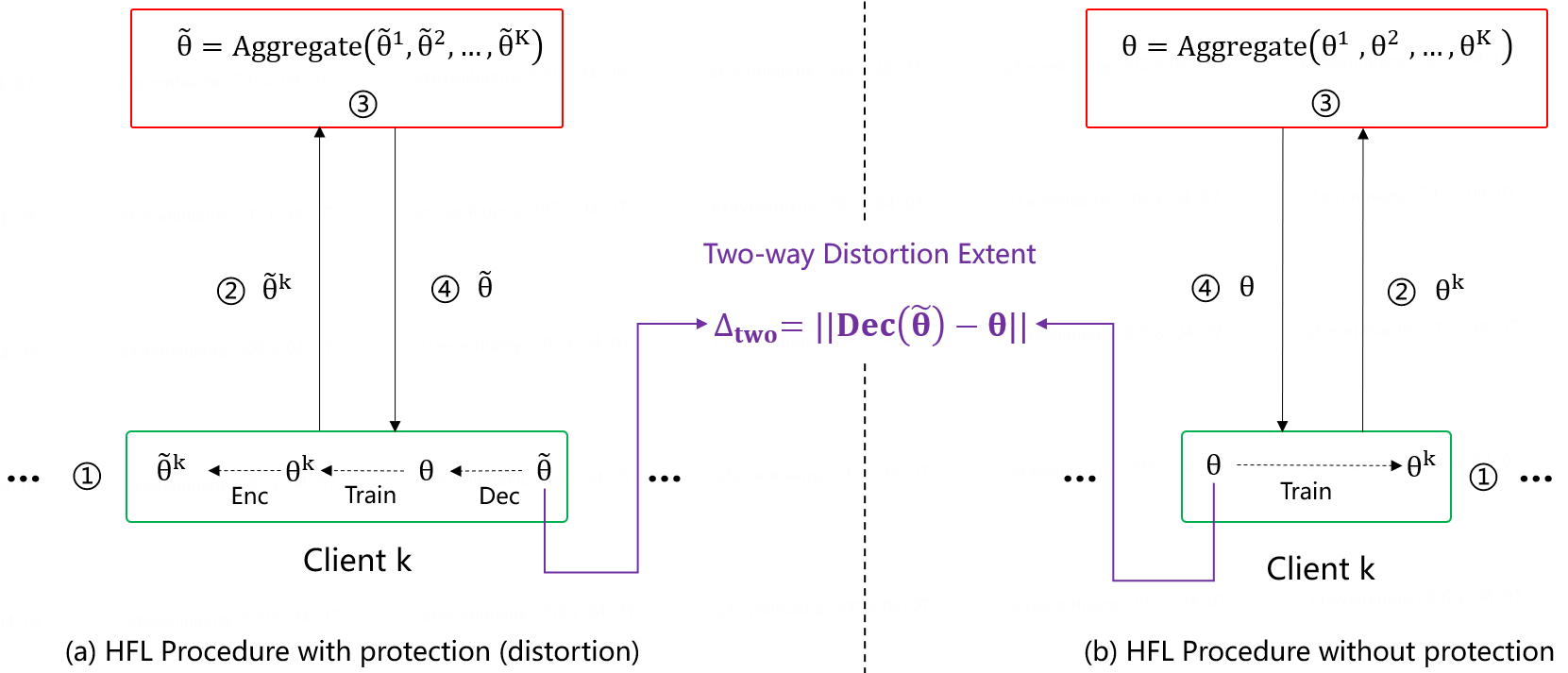
Figure 6: Illustration of two-way distortion extent. The left side is HFL training procedure with protection, and the right side is HFL training procedure without protection.

Definition 5.4 ($\lambda^{(k)}$-cover)

A $\lambda^{(k)}$-cover of $(\mathcal{X}_{\text{\rm prot}}^{(k)},\|\cdot\|_{2})$ is a point set $\{\mathbf{u}\}\subset\mathcal{X}_{\text{\rm prot}}^{(k)}$ such that for any $\mathbf{v}\in\mathcal{D}_{\text{\rm prot}}^{(k)}$, there exists $\mathbf{u}$ satisfies $\|\mathbf{u}-\mathbf{v}\|_{2}\leq\lambda^{(k)}$.

Now we analyze the generalization bounds against semi-honest attackers, with Randomization Mechanism be the protection mechanism. The following theorem measures the price of preserving privacy in terms of utility loss using the two-way distortion extent, assuming the training set of client $k$ consists of $|\mathcal{D}_{\text{\rm prot}}^{(k)}|$ independent and identically distributed samples that follows distribution $P$.

Theorem 5.1 (Utility Loss against Semi-honest Attackers)

Let $\theta\in\mathbb{R}^{d}$ represent the model parameter. Assume that $\max_{Z\in\mathcal{D}_{\text{\rm prot}}^{(k)}}|\mathcal{L}^{(k)}(\theta+\delta,Z)|\leq M^{(k)}$. We denote the empirical loss as $\mathcal{L}^{(k)}_{\text{emp}}(\theta,Z)=\frac{1}{m_{k}}\sum_{i=1}^{m_{k}}\mathcal{L}^{(k)}(\theta,Z_{i}^{(k)})$, and denote the expected loss as $\mathcal{L}^{(k)}_{\text{exp}}(\theta+\delta)=\mathbb{E}_{Z\sim P}[\mathcal{L}^{(k)}(\theta+\delta,Z)]$. With probability at least $1-\eta^{(k)}$,

$$\epsilon_{u}^{(k)} =|\mathcal{L}^{(k)}_{\text{exp}}(\theta+\delta)-\mathcal{L}^{(k)}_{\text{emp}}(\theta)|$$

$$\leq C\cdot\lambda^{(k)}+C\cdot\Delta_{\text{two}}+M^{(k)}\sqrt{\frac{2N^{(k)}\ln 2+2\ln(1/\eta^{(k)})}{|\mathcal{D}_{\text{\rm prot}}^{(k)}|}},$$ (20)

where $\mathcal{D}_{\text{\rm prot}}^{(k)}=\{Z_{1}^{(k)},\cdots,Z_{m_{k}}^{(k)}\}$ represents the training set of client $k$, $\lambda^{(k)}>\Delta_{\text{two}}$ represents a constant, $M^{(k)}$ is a constant, $N^{(k)}=(2d)^{2D/(\lambda^{(k)})^{2}+1}$ represents the covering number of $\lambda^{(k)}$-cover (Definition 5.4), $\Delta_{\text{two}}$ represents the two-way distortion extent (Definition 5.3), and $\|\delta\|=\Delta_{\text{two}}$.

5.2 Trade-off Between Utility, Privacy and Efficiency for General Protection Mechanisms

Before elaborating on the theoretical trade-off for the protection mechanism, we first derive the relationship between the two-way distortion extent and the uplink distortion extent. The following theorem illustrates the relationship between $\delta$ and $\Delta_{\text{two}}$, shows that $\Delta_{\text{up}}^{(k)}$ is equal to the norm of $\delta^{(k)}$, and further highlights the relationship between the uplink distortion extent and the two-way distortion extent.

Theorem 5.2

Let $\Delta_{\text{two}}$ denote the two-way distortion extent (Definition 5.3), and $\Delta_{\text{up}}^{(k)}$ denote the uplink distortion extent (Definition 4.3). The protector $k$ distorts the gradient according to Eq. (8), $\delta^{(k)}$ is introduced therein, and $\delta=\widetilde{\theta}-\theta$. Assume that $\text{Dec}(\widetilde{\theta})=\widetilde{\theta}$, then we have

$$\Delta_{\text{two}}=\|\delta\|,\quad\text{and}\quad\Delta_{\text{up}}^{(k)}=\|\delta^{(k)}\|.$$ (21)

Furthermore, assume that $\delta^{(1)}=\cdots=\delta^{(K)}$. Then we have

$$\Delta_{\text{two}}=\Delta_{\text{up}}^{(k)}.$$ (22)

Combining Theorem 4.1, Theorem 5.1 and Theorem 5.2, our main result is illustrated in the following theorem, which establishes a trade-off between utility, privacy and efficiency that acts as a paradigm for the design of protection mechanism against learning-based and semi-honest attacks. Please refer to Section F for the full proof.

Theorem 5.3 (Utility, Privacy and Efficiency Trade-off for General Protection Mechanisms)

Let $M^{(k)}$ be a constant satisfying that $\max_{Z\in\mathcal{D}_{\text{\rm prot}}^{(k)}}|\mathcal{L}(\theta+\delta,Z)|\leq M^{(k)}$. Assume that $\Delta_{\text{two}}=\Theta(\Delta_{\text{up}}^{(k)})$, then there exists a constant $L$, satisfying that $\Delta_{\text{two}}\leq L\cdot\Delta_{\text{up}}^{(k)}$. With probability at least $1-\eta^{(k)}-\sum_{k=1}^{K}\gamma^{(k)}$, we have that

$$\epsilon_{u}^{(k)} \leq C\cdot L\cdot\frac{1}{K}\sum_{k=1}^{K}\left(\frac{2D}{c_{a}}\cdot(1-\epsilon_{p}^{(k)})+\frac{2D}{c_{a}}\cdot\sqrt{\frac{\ln(1/\gamma^{(k)})}{\epsilon_{e}^{(k)}}}\right)$$

$$+M^{(k)}\sqrt{\frac{2N^{(k)}\ln 2+2\ln(1/\eta^{(k)})}{\epsilon_{e}^{(k)}}}.$$ (23)

5.3 Trade-off Analysis for Randomization Mechanism and Homomorphic Encryption Mechanism

In this section, we quantify the trade-off between utility, privacy and efficiency for two commonly-used privacy-preserving mechanisms: Randomization Mechanism (Geyer et al. (2017); Truex et al. (2020); Abadi et al. (2016)) and Homomorphic Encryption Mechanism (Gentry and Boneh (2009); Zhang et al. (2020a)).

5.3.1 Utility, Privacy and Efficiency Trade-off for Randomization Mechanism

Now we apply our theoretical framework to analyze the trade-off for Randomization Mechanism. Please refer to Appendix G for the full proof.

Theorem 5.4 (Utility, Privacy and Efficiency Trade-off for Randomization Mechanism)

Assume that $\max_{Z\in\mathcal{D}_{\text{\rm prot}}^{(k)}}|\mathcal{L}(\theta+\delta,Z)|\leq M^{(k)}$. For Randomization Mechanism, with probability at least $1-\eta^{(k)}-\sum_{k=1}^{K}\gamma^{(k)}$, we have that

$$\epsilon_{u}^{(k)} \leq(2+\rho)C\cdot\frac{1}{K}\sum_{k=1}^{K}\frac{2D}{c_{a}}\cdot(1-\epsilon_{p}^{(k)})+(2+\rho)C\cdot\frac{1}{K}\sum_{k=1}^{K}\frac{2D}{c_{a}}\cdot\sqrt{\frac{\ln(1/\gamma^{(k)})}{\epsilon_{e}^{(k)}}}$$

$$+M^{(k)}\sqrt{\frac{2N^{(k)}\ln 2+2\ln(1/\eta^{(k)})}{\epsilon_{e}^{(k)}}},$$ (24)

where $\rho>0$ represents a constant.

5.3.2 Utility-Efficiency Trade-off for Homomorphic Encryption Mechanism

Now we introduce the generalization bounds for Homomorphic Encryption (Gentry and Boneh (2009); Zhang et al. (2020a)). For Homomorphic Encryption Mechanism, the two-way distortion extent $\Delta_{\text{two}}=\|\text{Dec}(\widetilde{\theta})-\theta\|=0$. The following lemma illustrates the value of $\Delta_{\text{two}}$ for Homomorphic Encryption Mechanism. Please refer to Appendix H for the full proof.

Lemma 5.5

Let $\Delta_{\text{two}}$ denote the two-way distortion extent (Definition 5.3). For Homomorphic Encryption Mechanism, we have that

$$\Delta_{\text{two}}=0.$$ (25)

Note that $\Delta_{\text{up}}^{(k)}>0$ for Homomorphic Encryption Mechanism. Therefore, the assumption that $\Delta_{\text{two}}=\Theta(\Delta_{\text{up}}^{(k)})$ in Theorem 5.3 does not hold. Therefore, we do not provide trade-off analysis for the three factors via applying Theorem 5.3 for Homomorphic Encryption Mechanism. Instead, we provide a theoretical trade-off analysis for utility and efficiency, as is illustrated in the following theorem.

Theorem 5.6 (Utility-Efficiency Trade-off for Homomorphic Encryption Mechanism)

Let $\theta\in\mathbb{R}^{d}$ represent the model parameter. Assume that $\max_{Z\in\mathcal{D}_{\text{\rm prot}}^{(k)}}|\mathcal{L}^{(k)}(\theta+\delta,Z)|\leq M^{(k)}$. We denote the empirical loss as $\mathcal{L}^{(k)}_{\text{emp}}(\theta,Z)=\frac{1}{m_{k}}\sum_{i=1}^{m_{k}}\mathcal{L}^{(k)}(\theta,Z_{i}^{(k)})$, and denote the expected loss as $\mathcal{L}^{(k)}_{\text{exp}}(\theta+\delta)=\mathbb{E}_{Z\sim P}[\mathcal{L}^{(k)}(\theta+\delta,Z)]$. With probability at least $1-\eta^{(k)}$,

$$\epsilon_{u}^{(k)} =|\mathcal{L}^{(k)}_{\text{exp}}(\theta+\delta)-\mathcal{L}^{(k)}_{\text{emp}}(\theta)|$$

$$\leq C\cdot\lambda^{(k)}+M^{(k)}\sqrt{\frac{2N^{(k)}\ln 2+2\ln(1/\eta^{(k)})}{|\mathcal{D}_{\text{\rm prot}}^{(k)}|}},$$ (26)

where $\mathcal{D}_{\text{\rm prot}}^{(k)}=\{Z_{1}^{(k)},\cdots,Z_{m_{k}}^{(k)}\}$ represents the training set of client $k$, $\lambda^{(k)}>\Delta_{\text{two}}$ represents a constant, $M^{(k)}$ is a constant, $N^{(k)}=(2d)^{2D/(\lambda^{(k)})^{2}+1}$ represents the covering number of $\lambda^{(k)}$-cover (Definition 5.4), $\Delta_{\text{two}}$ represents the two-way distortion extent (Definition 5.3), and $\|\delta\|=\Delta_{\text{two}}=0$.

6 Discussions

The challenge of increasing the effectiveness and efficiency of federated learning has prompted the development of a number of strategies in this area, which are classified into the following categories:

• Improving Model Utility [C1]: Personalization (Hard et al. (2018); Wang et al. (2019)), Fine-tuning and Domain Adaptation (Mansour et al. (2009); Ben-David et al. (2010); Mansour et al. (2021); Cortes and Mohri (2014));

• Improving Privacy Guarantee [C2]: Randomization (Geyer et al. (2017); Truex et al. (2020); Abadi et al. (2016)), Sparsity (Shokri and Shmatikov (2015); Gupta and Raskar (2018); Thapa et al. (2020)) and Homomorphic Encryption (HE) (Gentry and Boneh (2009); Zhang et al. (2020a));

• Improving Training Efficiency [C3]: Accelerated Mini-batch SGD (Cotter et al. (2011); Dekel et al. (2012); Lan (2012); Stich (2018)), SCAFFOLD (Karimireddy et al. (2020)).

We propose a unifying framework for analyzing the trade-off between privacy, utility and efficiency for various protection mechanisms including Randomization (Geyer et al. (2017); Truex et al. (2020); Abadi et al. (2016)) and Homomorphic Encryption (HE) (Gentry and Boneh (2009); Zhang et al. (2020a)). Within this framework, we provide a unified metric so that different protection and attacking mechanisms are comparable via sample complexity. We derive theoretical bounds for a myriad of federated learning approaches against semi-honest attackers. Specifically, Theorem 5.3 and Theorem 4.2 shed light on algorithmic designs of protection mechanisms against semi-honest attackers with Learning Phase 1 and 2 separately. Theorem 5.3 shows that the preservation of privacy [C2] (efficiency [C3]) may be fundamentally at odds with the goal of improving utility [C1], and provides an explanation for the decline in model utility [C1] when privacy [C2] (efficiency [C3])-preserving strategies are implemented in real-world settings. Theorem 4.2 could serve as a basis for the algorithmic proposal of a novel protection mechanism, which assures PAC-learnability for any semi-honest attackers with Learning Phase 2 could not be achieved.

Implications on Designing a Protection Mechanism Against Phase-1 Attacker

We use Randomization Mechanism as an example, and focus on the theoretical result illustrated in Theorem 5.4 (an application of Theorem 5.3 on Randomization Mechanism). Theorem 5.4 provides an avenue to evaluate the number of samples required for the protector to achieve a utility loss of at most $\alpha$ with high probability, given the requirement on privacy leakage. Please refer to Appendix I for the full proof.

Corollary 1 (Private PAC Learning)

Let $\mathcal{X}$ represent the feature set, and $\mathcal{Y}$ represent the label set. Let $\epsilon_{p}$ represent the amount of privacy leaked to the learning-based and semi-honest attackers. For any $\alpha>c_{2}(1-\epsilon_{p})$, given $n=\Theta\left(\frac{\ln(\frac{1}{\eta})}{(\alpha-c_{2}(1-\epsilon_{p}))^{2}}\right)$ i.i.d. samples from any distribution $P$ on $\mathcal{X}\times\mathcal{Y}$, with probability at least $1-\eta$, the utility loss of the protector is at most $\alpha$, as is shown in the following equation:

$${\rm Pr}(\epsilon_{u}\leq\alpha)\geq 1-\eta.$$ (27)

Implications on Designing a Protection Mechanism Against Phase-2 Attacker

Theorem 4.2 implies that the protector could guarantee not PAC learnable for any semi-honest attacker with Learning Phase 2 by adjusting the distortion extent and the size of the training set, as is illustrated in the following corollary.

Corollary 2 (Not PAC Learnable)

If the uplink distortion extent of protector $k$ satisfies that $\Delta_{\text{up}}^{(k)}>\ln\left(\frac{|\mathcal{D}_{\text{\rm prot}}^{(k)}|}{1-\epsilon}\right)$, then the classification problem associated with protector $k$ is not $(\epsilon,\delta)$-PAC learnable for any semi-honest attacker.

It is worth noting that $|\mathcal{D}_{\text{\rm prot}}^{(k)}|$ and $\Delta_{\text{up}}^{(k)}$ are both determined by the protector, which facilitates the proposal of a novel protection mechanism, and at the same time guarantees that any learning-based and semi-honest attackers could not achieve PAC-learnability.

7 Conclusion and Future Work

In this work, we model the performance of the protector and the attacker from the perspective of PAC learning, and evaluate the cost of both the protector and the attacker via sample complexity in a unified manner. Within the proposed unified framework, we measure multiple objectives including privacy, utility and efficiency along the unified evaluation metric. For the learning-based and semi-honest attacker, we analyze how many samples are needed to achieve PAC learnability (see exponential lower bound). For the defender, we analyze how many samples are needed to achieve required utility loss with high probability in the framework of PAC learning (see upper bound for utility loss). The unifying framework along with the unified measurements can further inspire the design of smart privacy-preserving federated learning algorithms that deal with the trade-offs in the solution space. We also provide an upper bound for the privacy leakage of the semi-honest attacker. The bounds for utility loss and privacy leakage in the PAC framework further establishes a trade-off between utility, privacy and efficiency. Our analysis is applicable to distinct protection mechanisms including Randomization Mechanism and Homomorphic Encryption Mechanism against learning-based and semi-honest attackers. Our theoretical analysis serves as a basis for the algorithmic proposal of a novel protection mechanism. It is an intriguing direction to see if our techniques could be used to quantify theoretical trade-offs against malicious attackers.

Appendix A Notations

The notations used throughout this article is shown in the following table.

Table 1: Table of Notation

Notation	Meaning
$\epsilon_{p}^{(k)}$	privacy leakage of client $k$
$\epsilon_{u}^{(k)}$	utility loss of client $k$
$\mathcal{L}$	loss function
$g$	the original gradient
$\widetilde{g}$	the distorted gradient
$\Delta$	distortion extent
$\theta$	the original model parameter
$\widetilde{\theta}$	the distorted model parameter
$\mathcal{X}$	a set of instances
$\mathcal{Y}$	a set of labels
$P$	distribution over instances $\mathcal{X}$

Appendix B Analysis for Theorem 4.1

Lemma B.1 (Chernoff-Hoeffding Inequality)

Let $X_{1},X_{2},\dots,X_{t}$ be i.i.d. random variables supported on $[0,1]$. For any positive number $\epsilon$, we have

$$\Pr\left(\left|\frac{1}{t}\sum_{i=1}^{t}X_{i}-E\left[\frac{1}{t}\sum_{i=1}^{t}X_{i}\right]\right|\geq\epsilon\right)\leq 2\exp\left(-2t\epsilon^{2}\right).$$ (28)

Theorem B.2 (Upper Bound for Privacy Leakage)

Let Assumption 4.1 and Assumption 4.2 hold. Assume that $\Delta_{\text{up}}^{(k)}\geq\frac{2c_{2}\cdot c_{b}}{c_{a}\sqrt{T}}$, where $T$ represents the total number of the learning rounds of the semi-honest attacker, $c_{a},c_{2}$ and $c_{b}$ are introduced in Assumption 4.1 and Assumption 4.2. With probability at least $1-\gamma^{(k)}$, we have

$$\epsilon_{p}^{(k)}\leq 1+\sqrt{\frac{\ln(2/\gamma^{(k)})}{2|\mathcal{D}_{\text{\rm prot}}^{(k)}|}}-\frac{c_{a}}{2D}\cdot\Delta_{\text{up}}^{(k)}.$$ (29)

Proof  Let $X_{t,i}^{(k)}$ represent the $i$-th data of the protector $k$ that is recovered by the attacker at the $t$-th round of the optimization algorithm, and $X_{i}^{(k)}$ represent the $i$-th original data of the protector $k$. Let $\mathcal{D}_{\text{\rm attack}}^{(k)}=\{(X_{1}^{(k)},Y_{1}^{(k)}),\cdots,(X_{m_{k}}^{(k)},Y_{m_{k}}^{(k)})\}$ represent the mini-batch that generates $\widetilde{g}$. We have that

$$\frac{1}{|\mathcal{D}_{\text{\rm attack}}^{(k)}|}\sum_{i=1}^{|\mathcal{D}_{\text{\rm attack}}^{(k)}|}\frac{1}{T}\sum_{t=1}^{T}||X_{t,i}^{(k)}-X_{i}^{(k)}||$$

$$\geq\frac{1}{|\mathcal{D}_{\text{\rm attack}}^{(k)}|}\sum_{i=1}^{|\mathcal{D}_{\text{\rm attack}}^{(k)}|}\frac{1}{T}\sum_{t=1}^{T}||\widetilde{X}_{i}^{(k)}-X_{i}^{(k)}||-\frac{1}{|\mathcal{D}_{\text{\rm attack}}^{(k)}|}\sum_{i=1}^{|\mathcal{D}_{\text{\rm attack}}^{(k)}|}\frac{1}{T}\sum_{t=1}^{T}||X_{t,i}^{(k)}-\widetilde{X}_{i}^{(k)}||$$

$$\geq c_{a}\cdot\frac{1}{T}\sum_{t=1}^{T}\frac{1}{|\mathcal{D}_{\text{\rm attack}}^{(k)}|}\sum_{i=1}^{|\mathcal{D}_{\text{\rm attack}}^{(k)}|}||\nabla\mathcal{L}(\theta,\widetilde{X}_{i}^{(k)},Y_{i}^{(k)})-\nabla\mathcal{L}(\theta,X_{i}^{(k)},Y_{i}^{(k)})||$$

$$\quad-c_{b}\cdot\frac{1}{T}\sum_{t=1}^{T}\frac{1}{|\mathcal{D}_{\text{\rm attack}}^{(k)}|}\sum_{i=1}^{|\mathcal{D}_{\text{\rm attack}}^{(k)}|}||\nabla\mathcal{L}(\theta,X_{t,i}^{(k)},Y_{i}^{(k)})-\nabla\mathcal{L}(\theta,\widetilde{X}_{i}^{(k)},Y_{i}^{(k)})||$$

$$\geq c_{a}\cdot\frac{1}{T}\sum_{t=1}^{T}||\frac{1}{|\mathcal{D}_{\text{\rm attack}}^{(k)}|}\sum_{i=1}^{|\mathcal{D}_{\text{\rm attack}}^{(k)}|}(\nabla\mathcal{L}(\theta,\widetilde{X}_{i}^{(k)},Y_{i}^{(k)})-\nabla\mathcal{L}(\theta,X_{i}^{(k)},Y_{i}^{(k)}))||$$

$$\quad-c_{b}\cdot\frac{1}{T}\sum_{t=1}^{T}\frac{1}{|\mathcal{D}_{\text{\rm attack}}^{(k)}|}\sum_{i=1}^{|\mathcal{D}_{\text{\rm attack}}^{(k)}|}||\nabla\mathcal{L}(\theta,X_{t,i}^{(k)},Y_{i}^{(k)})-\nabla\mathcal{L}(\theta,\widetilde{X}_{i}^{(k)},Y_{i}^{(k)})||$$

$$=c_{a}\cdot\Delta_{\text{up}}^{(k)}-c_{b}\cdot\frac{1}{T}\sum_{t=1}^{T}\frac{1}{|\mathcal{D}_{\text{\rm attack}}^{(k)}|}\sum_{i=1}^{|\mathcal{D}_{\text{\rm attack}}^{(k)}|}||\nabla\mathcal{L}(\theta,X_{t,i}^{(k)},Y_{i}^{(k)})-\nabla\mathcal{L}(\theta,\widetilde{X}_{i}^{(k)},Y_{i}^{(k)})||,$$ (30)

where the second inequality is due to $||\widetilde{X}_{i}^{(k)}-X_{i}^{(k)}||\geq c_{a}||\nabla\mathcal{L}(\theta,\widetilde{X}_{i}^{(k)},Y_{i}^{(k)})-\nabla\mathcal{L}(\theta,X_{i}^{(k)},Y_{i}^{(k)})||$ and $||X_{t,i}^{(k)}-\widetilde{X}_{i}^{(k)}||\leq c_{b}||\nabla\mathcal{L}(\theta,X_{t,i}^{(k)},Y_{i}^{(k)})-\nabla\mathcal{L}(\theta,\widetilde{X}_{i}^{(k)},Y_{i}^{(k)})||$, the third inequality is due to the triangle inequality ($\|a\|+\|b\|\geq\|a+b\|$), and the last equality is due to $\|\frac{1}{|\mathcal{D}_{\text{\rm attack}}^{(k)}|}\sum_{i=1}^{|\mathcal{D}_{\text{\rm attack}}^{(k)}|}(\nabla\mathcal{L}(\theta,\widetilde{X}_{i}^{(k)},Y_{i}^{(k)})-\nabla\mathcal{L}(\theta,X_{i}^{(k)},Y_{i}^{(k)}))\|=\|\delta^{(k)}\|=\Delta_{\text{up}}^{(k)}$ from Lemma E.2. Now we bound the second term of Eq. (30). We have that

$$c_{a}\cdot\Delta_{\text{up}}^{(k)}-c_{b}\cdot\frac{1}{T}\sum_{t=1}^{T}\frac{1}{|\mathcal{D}_{\text{\rm attack}}^{(k)}|}\sum_{i=1}^{|\mathcal{D}_{\text{\rm attack}}^{(k)}|}||\nabla\mathcal{L}(\theta,X_{t,i}^{(k)},Y_{i}^{(k)})-\nabla\mathcal{L}(\theta,\widetilde{X}_{i}^{(k)},Y_{i}^{(k)})||$$

$$\geq c_{a}\Delta_{\text{up}}^{(k)}-c_{2}\cdot c_{b}T^{-\frac{1}{2}}$$

$$\geq\frac{c_{a}}{2}\cdot\Delta_{\text{up}}^{(k)},$$

where the second inequality is due to $c_{a}\Delta_{\text{up}}^{(k)}\geq 2c_{2}\cdot c_{b}T^{-\frac{1}{2}}$ from our assumption.
Using Hoeffding’s inequality (Lemma B.1), we have that with probability at least $1-\delta$,

$$\left|\frac{1}{|\mathcal{D}_{\text{\rm attack}}^{(k)}|}\sum_{i=1}^{|\mathcal{D}_{\text{\rm attack}}^{(k)}|}X_{i}-\mathbb{E}\left[\frac{1}{|\mathcal{D}_{\text{\rm attack}}^{(k)}|}\sum_{i=1}^{|\mathcal{D}_{\text{\rm attack}}^{(k)}|}X_{i}\right]\right|\leq\sqrt{\frac{\ln(2/\gamma^{(k)})}{2|\mathcal{D}_{\text{\rm attack}}^{(k)}|}},$$ (31)

where $|\mathcal{D}_{\text{\rm attack}}^{(k)}|$ represents the size of the mini-batch (the training set of the attacker).
Therefore, with probability at least $1-\delta$, we have

$$\frac{1}{|\mathcal{D}_{\text{\rm attack}}^{(k)}|}\sum_{i=1}^{|\mathcal{D}_{\text{\rm attack}}^{(k)}|}\frac{1}{T}\sum_{t=1}^{T}\frac{||X_{t,i}^{(k)}-X_{i}^{(k)}||}{D}$$

$$\leq\mathbb{E}\left[\frac{1}{|\mathcal{D}_{\text{\rm attack}}^{(k)}|}\sum_{i=1}^{|\mathcal{D}_{\text{\rm attack}}^{(k)}|}\frac{1}{T}\sum_{t=1}^{T}\frac{||X_{t,i}^{(k)}-X_{i}^{(k)}||}{D}\right]+\sqrt{\frac{\ln(2/\gamma^{(k)})}{2|\mathcal{D}_{\text{\rm attack}}^{(k)}|}}$$

$$=1-\epsilon_{p}^{(k)}+\sqrt{\frac{\ln(2/\gamma^{(k)})}{2|\mathcal{D}_{\text{\rm attack}}^{(k)}|}}.$$

Therefore, we have

$$1-\epsilon_{p}^{(k)}+\sqrt{\frac{\ln(2/\gamma^{(k)})}{2|\mathcal{D}_{\text{\rm attack}}^{(k)}|}} \geq\frac{1}{|\mathcal{D}_{\text{\rm attack}}^{(k)}|}\sum_{i=1}^{|\mathcal{D}_{\text{\rm attack}}^{(k)}|}\frac{1}{T}\sum_{t=1}^{T}\frac{||X_{t,i}^{(k)}-X_{i}^{(k)}||}{D}$$

$$\geq\frac{c_{a}\Delta_{\text{up}}^{(k)}}{2D}.$$

Therefore,

$$\Delta_{\text{up}}^{(k)}\leq\frac{2D}{c_{a}}\cdot(1-\epsilon_{p}^{(k)})+\frac{2D}{c_{a}}\cdot\sqrt{\frac{\ln(2/\gamma^{(k)})}{2|\mathcal{D}_{\text{\rm attack}}^{(k)}|}}.$$ (32)

Notice that

$$|\mathcal{D}_{\text{\rm attack}}^{(k)}|=|\mathcal{D}_{\text{\rm prot}}^{(k)}|.$$ (33)

Therefore, we have that

$$\frac{c_{a}}{2D}\cdot\Delta_{\text{up}}^{(k)}\leq 1-\epsilon_{p}^{(k)}+\sqrt{\frac{\ln(2/\gamma^{(k)})}{2|\mathcal{D}_{\text{\rm prot}}^{(k)}|}}.$$ (34)

Therefore, we have

$$\epsilon_{p}^{(k)}\leq 1+\sqrt{\frac{\ln(2/\gamma^{(k)})}{2|\mathcal{D}_{\text{\rm prot}}^{(k)}|}}-\frac{c_{a}}{2D}\cdot\Delta_{\text{up}}^{(k)}.$$ (35)

 

Appendix C Analysis for Theorem 4.2

We provide an exponential lower bound for the sample complexity of the attacker. With a sublinear amount of distortion of the model parameter, at least an exponentially amount of samples are required for the attacker to achieve PAC learnability. The high-level ideas are

• First, the risk of a classifier generated by any learning algorithm with sub-exponential sample complexity is at least $\Omega\left(\frac{1}{|\mathcal{D}_{\text{\rm attack}}^{(k)}|}\right)$, where $|\mathcal{D}_{\text{\rm attack}}^{(k)}|$ represents the number of samples.

• Second, we show that the original risk turns into a rather large adversarial risk with a certain amount of distortion, which contradicts the assumption of PAC learnability.

Now we are ready to provide the analysis for this theorem that is motivated by Diochnos et al. (2019).

Notice that the distance between any data from the original dataset and that from the inferred dataset is about $\Theta(\Delta^{(k)})$.

Theorem C.1

Let $\Delta_{\text{up}}^{(k)}$ denote the uplink distortion extent (Definition 4.3), and $\Delta^{(k)}=\max_{i}||\widetilde{X}^{(k)}_{i}-X^{(k)}_{i}||$. Then we have that,

$$\Delta^{(k)}\geq c_{a}\Delta_{\text{up}}^{(k)}.$$ (36)

Proof  We denote $g^{(k)}$ as the original gradient of client $k$, and $\widetilde{g}^{(k)}$ as the distorted gradient uploaded from client $k$ to the server. Recall that $g^{(k)}=\frac{1}{|\mathcal{D}_{\text{\rm attack}}^{(k)}|}\sum_{i=1}^{|\mathcal{D}_{\text{\rm attack}}^{(k)}|}\nabla\mathcal{L}(\theta,X_{i}^{(k)},Y_{i}^{(k)})$, and $\widetilde{g}^{(k)}=\frac{1}{|\mathcal{D}_{\text{\rm attack}}^{(k)}|}\sum_{i=1}^{|\mathcal{D}_{\text{\rm attack}}^{(k)}|}\nabla\mathcal{L}(\theta,\widetilde{X}_{i}^{(k)},Y_{i}^{(k)})$. The distortion extent of client $k$

$$\Delta_{\text{up}}^{(k)}=\|\widetilde{g}^{(k)}-g^{(k)}\|.$$ (37)

From Assumption 4.1, we have that

$$||\widetilde{X}^{(k)}_{i}-X^{(k)}_{i}|| \geq c_{a}||\nabla\mathcal{L}(\theta,\widetilde{X}^{(k)}_{i},Y_{i})-\nabla\mathcal{L}(\theta,X^{(k)}_{i},Y_{i})||.$$ (38)

Therefore, we have

$$\max_{i}||\widetilde{X}^{(k)}_{i}-X^{(k)}_{i}|| \geq\frac{1}{|\mathcal{D}_{\text{\rm attack}}^{(k)}|}\sum_{i=1}^{|\mathcal{D}_{\text{\rm attack}}^{(k)}|}c_{a}||\nabla\mathcal{L}(\theta,\widetilde{X}_{i}^{(k)},Y_{i})-\nabla\mathcal{L}(\theta,X_{i}^{(k)},Y_{i})||$$

$$\geq c_{a}\big{\|}\frac{1}{|\mathcal{D}_{\text{\rm attack}}^{(k)}|}\sum_{i=1}^{|\mathcal{D}_{\text{\rm attack}}^{(k)}|}\nabla\mathcal{L}(\theta,\widetilde{X}_{i}^{(k)},Y_{i}^{(k)})-\frac{1}{|\mathcal{D}_{\text{\rm attack}}^{(k)}|}\sum_{i=1}^{|\mathcal{D}_{\text{\rm attack}}^{(k)}|}\nabla\mathcal{L}(\theta,X_{i}^{(k)},Y_{i}^{(k)})\big{\|}$$

$$=c_{a}||\widetilde{g}^{(k)}-g^{(k)}||,$$

where the second inequality is due to the triangle inequality ($\|a\|+\|b\|\geq\|a+b\|$).
Therefore,

$$\Delta^{(k)}=\max_{i}||\widetilde{X}^{(k)}_{i}-X^{(k)}_{i}||\geq c_{a}\|\widetilde{g}^{(k)}-g^{(k)}\|=c_{a}\Delta_{\text{up}}^{(k)}.$$ (39)

Therefore, we have that

$$\Delta^{(k)}\geq c_{a}\Delta_{\text{up}}^{(k)}.$$ (40)

 

Definition C.1 (Normal Levy Family)

Let $d$ represent the dimension. A family of metric probability spaces with concentration function $\alpha_{d}(\cdot)$ is called a normal Levy family, if there exist $k_{1},k_{2}$ satisfying that

$$\alpha_{d}(c)\leq k_{1}\cdot e^{-k_{2}\cdot c^{2}/d}.$$ (41)

The intuition of the following lemma is: if the number of samples is not large enough, with high constant probability, all the instances in the training set could not provide any information for the learner to distinguish classifier $c_{1}$ from classifier $c_{2}$. Then, with high constant probability, we can provide a lower bound for the original risk of the learner.

Lemma C.2 (Lower Bound for Original Risk)

Let Assumption 4.3 hold. Assume $1>\delta>0.5$. Let $|\mathcal{D}_{\text{\rm attack}}^{(k)}|=2^{O(\Delta^{(k)})}$, then with probability at least $1-\delta$, we have that

$$\text{\rm Risk}(h,c)\geq\frac{a_{1}(2\delta-1)}{4a_{2}|\mathcal{D}_{\text{\rm attack}}^{(k)}|},$$ (42)

where $a_{1},a_{2}>0$ represent two constants.

Proof  Recall Assumption 4.3 implies that there exist two classifiers $c_{1},c_{2}$ (from $\mathcal{X}$ to $\mathcal{Y}$) satisfying that $\Pr_{\widetilde{X}\sim\widetilde{P}}[c_{1}(\widetilde{X})\neq c_{2}(\widetilde{X})]=\Theta(\epsilon)$, for all $1\geq\epsilon\geq 2^{-\Theta(d)}$.

We define $\text{\rm Diff}(c_{1},c_{2})=\{\widetilde{X}\in\mathcal{X}|c_{1}(\widetilde{X})\neq c_{2}(\widetilde{X})\}$. Note that $|\mathcal{D}_{\text{\rm attack}}^{(k)}|=2^{O(\Delta^{(k)})}$. From Assumption 4.3 and $\frac{\gamma}{2|\mathcal{D}_{\text{\rm attack}}^{(k)}|}\geq 2^{-\Theta(\Delta^{(k)})}\geq 2^{-\Theta(d)}$, there exist two classifiers $c_{1},c_{2}$ such that

$$\frac{a_{2}\gamma}{|\mathcal{D}_{\text{\rm attack}}^{(k)}|}\geq\Pr_{\widetilde{X}\sim\widetilde{P}}[\widetilde{X}\in\text{\rm Diff}(c_{1},c_{2})]\geq\frac{a_{1}\gamma}{2|\mathcal{D}_{\text{\rm attack}}^{(k)}|},$$ (43)

where $a_{1},a_{2}>0$ represent two constants.

Assume the learner has a total of $|\mathcal{D}_{\text{\rm attack}}^{(k)}|$ i.i.d. samples, which is denoted as the training set $\mathcal{S}$. Let $\mathcal{X}=\{X_{1},X_{2},\cdots,X_{|\mathcal{D}_{\text{\rm attack}}^{(k)}|}\}$, $\mathcal{E}_{i}=\{X_{i}\notin\text{\rm Diff}(c_{1},c_{2})\}$, and $\mathcal{E}=\{\forall X\in\mathcal{X}|X\notin\text{\rm Diff}(c_{1},c_{2})\}$. Therefore,

$$\Pr[\bar{\mathcal{E}}_{i}]\leq\frac{a_{2}\gamma}{|\mathcal{D}_{\text{\rm attack}}^{(k)}|}.$$ (44)

Then, the probability that event $\mathcal{E}$ holds is

$$\Pr[\mathcal{E}] =\Pr[\mathcal{E}_{1}\cap\cdots\cap\mathcal{E}_{|\mathcal{D}_{\text{\rm attack}}^{(k)}|}]$$ (45)

$$=1-\Pr[\bar{\mathcal{E}}_{1}\cup\cdots\cup\bar{\mathcal{E}}_{|\mathcal{D}_{\text{\rm attack}}^{(k)}|}]$$ (46)

$$\geq 1-\sum_{i}\Pr[\bar{\mathcal{E}}_{i}]$$ (47)

$$\geq 1-|\mathcal{D}_{\text{\rm attack}}^{(k)}|\cdot\frac{a_{2}\gamma}{|\mathcal{D}_{\text{\rm attack}}^{(k)}|}$$ (48)

$$=1-a_{2}\gamma.$$ (49)

Therefore,

$$\Pr[\mathcal{E}]\geq 1-a_{2}\gamma=2(1-\delta).$$ (50)

If all the samples in the training set do not belong to $\text{\rm Diff}(c_{1},c_{2})$ (which corresponds to $\mathcal{E}$), then the learner could not distinguish $c_{1}$ from $c_{2}$. Let $c$ be a random classifier that is sampled from $\{c_{1},c_{2}\}$. With probability at least $1-\delta$,

$$\text{\rm Risk}(h,c) =\Pr_{\widetilde{X}\sim\widetilde{P}}[h(\widetilde{X})\neq c(\widetilde{X})]$$

$$\geq\frac{1}{2}\cdot\Pr_{\widetilde{X}\sim\widetilde{P}}[\widetilde{X}\in\text{\rm Diff}(c_{1},c_{2})]$$

$$\geq\frac{a_{1}\gamma}{4|\mathcal{D}_{\text{\rm attack}}^{(k)}|}$$

$$=\frac{a_{1}(2\delta-1)}{4a_{2}|\mathcal{D}_{\text{\rm attack}}^{(k)}|}.$$

 

The following lemma measures the relationship between the risk and the adversarial risk using the distortion extent.

Lemma C.3 (Relationship between Risk and Adversarial Risk)

Let $\mathcal{B}$ represent a Borel set. If the original risk $\Pr_{\widetilde{X}\sim\widetilde{P}}[h(\widetilde{X})\neq c(\widetilde{X})]>1-\inf\{\Pr_{\widetilde{X}\sim\widetilde{P}}[d(\widetilde{X},\mathcal{B})\leq\Delta_{1}^{(k)}]|\Pr_{\widetilde{X}\sim\widetilde{P}}[\widetilde{X}\in\mathcal{B}]\geq\frac{1}{2}\}$, and the distortion extent is $\Delta_{1}^{(k)}+\Delta_{2}^{(k)}$, then the adversarial risk is larger than $1-\gamma$, where $\gamma>1-\inf\{\Pr_{\widetilde{X}\sim\widetilde{P}}[d(\widetilde{X},\mathcal{B})\leq\Delta_{2}^{(k)}]|\Pr_{\widetilde{X}\sim\widetilde{P}}[\widetilde{X}\in\mathcal{B}]\geq\frac{1}{2}\}$.

Proof  The risk of a classifier $h\in\mathcal{H}$ is defined as

$$\text{\rm Risk}(h,c)=\Pr_{\widetilde{X}\sim\widetilde{P}}[h(\widetilde{X})\neq c(\widetilde{X})].$$ (51)

We denote $\text{\rm Diff}(h,c)=\{X\in\mathcal{X}|h(X)\neq c(X)\}$, and $\text{\rm Diff}(h,c,\Delta^{(k)})=\{X\in\mathcal{X}|d(X,\text{\rm Diff}(h,c))\leq\Delta^{(k)}\}$. The adversarial risk is defined as

$$\text{\rm AdvRisk}(h,c,\Delta^{(k)}) =\Pr_{\widetilde{X}\sim\widetilde{P}}[\exists X\in\mathcal{X}:d(X,\widetilde{X})\leq\Delta^{(k)},h(X)\neq c(X)]$$ (52)

$$=\Pr_{\widetilde{X}\sim\widetilde{P}}[d(\widetilde{X},\text{\rm Diff}(h,c))\leq\Delta^{(k)}].$$ (53)

Assume that $\text{\rm AdvRisk}(h,c,\Delta_{1}^{(k)})\leq\frac{1}{2}$, and denote $\mathcal{B}_{0}=\mathcal{X}\setminus\text{\rm Diff}(h,c,\Delta_{1}^{(k)})$. Then, it holds that

$$\Pr_{\widetilde{X}\sim\widetilde{P}}[\widetilde{X}\in\mathcal{B}_{0}] =\Pr_{\widetilde{X}\sim\widetilde{P}}[d(\widetilde{X},\text{\rm Diff}(h,c))>\Delta_{1}^{(k)}]$$

$$=1-\Pr_{\widetilde{X}\sim\widetilde{P}}[\exists X\in\mathcal{X}:d(X,\widetilde{X})\leq\Delta_{1}^{(k)},h(X)\neq c(X)]$$

$$=1-\text{\rm AdvRisk}(h,c,\Delta_{1}^{(k)})$$

$$\geq\frac{1}{2}.$$

We denote $\mathcal{B}_{1}=\{X\in\mathcal{X}|d(X,\mathcal{B}_{0})\leq\Delta_{1}^{(k)}\}$. We know that

$$\Pr_{\widetilde{X}\sim\widetilde{P}}[\widetilde{X}\in\mathcal{B}_{1}] =\Pr_{\widetilde{X}\sim\widetilde{P}}[d(\widetilde{X},\mathcal{B}_{0})\leq\Delta_{1}^{(k)}]$$ (54)

$$\geq\inf\{\Pr_{\widetilde{X}\sim\widetilde{P}}[d(\widetilde{X},\mathcal{B})\leq\Delta_{1}^{(k)}]|\Pr_{\widetilde{X}\sim\widetilde{P}}[\widetilde{X}\in\mathcal{B}]\geq\frac{1}{2}\}$$ (55)

$$>1-\Pr_{\widetilde{X}\sim\widetilde{P}}[h(\widetilde{X})\neq c(\widetilde{X})]$$ (56)

$$=\Pr_{\widetilde{X}\sim\widetilde{P}}[h(\widetilde{X})=c(\widetilde{X})],$$ (57)

where the first inequality is due to $\Pr_{\widetilde{X}\sim\widetilde{P}}[\widetilde{X}\in\mathcal{B}_{0}]\geq\frac{1}{2}$, and the second inequality is due to $\Pr_{\widetilde{X}\sim\widetilde{P}}[h(\widetilde{X})\neq c(\widetilde{X})]>1-\inf\{\Pr_{\widetilde{X}\sim\widetilde{P}}[d(\widetilde{X},\mathcal{B})\leq\Delta_{1}^{(k)}]|\Pr_{\widetilde{X}\sim\widetilde{P}}[\widetilde{X}\in\mathcal{B}]\geq\frac{1}{2}\}$ from our assumption.
Therefore, there exist $\widehat{X}\in\mathcal{X}\setminus\text{\rm Diff}(h,c,\Delta_{1}^{(k)})$ and $\widetilde{X}\in\text{\rm Diff}(h,c)\cap\mathcal{B}_{1}$ such that

$$d(\widetilde{X},\hat{X})\leq\Delta_{1}^{(k)}.$$ (58)

$\widetilde{X}\in\text{\rm Diff}(h,c)$ further implies that

$$\widehat{X}\in\text{\rm Diff}(h,c,\Delta_{1}^{(k)}),$$ (59)

which leads to a contradiction.
Therefore, we have that

$$\text{\rm AdvRisk}(h,c,\Delta_{1}^{(k)}) =\Pr_{\widetilde{X}\sim\widetilde{P}}[d(\widetilde{X},\text{\rm Diff}(h,c))\leq\Delta_{1}^{(k)}]$$ (60)

$$=\Pr_{\widetilde{X}\sim\widetilde{P}}[\widetilde{X}\in\text{\rm Diff}(h,c,\Delta_{1}^{(k)})]$$ (61)

$$>\frac{1}{2}.$$ (62)

Let $\mathcal{B}_{2}=\{X\in\mathcal{X}|d(X,\text{\rm Diff}(h,c,\Delta_{1}^{(k)}))\leq\Delta_{2}^{(k)}\}$. From $\gamma>1-\inf\{\Pr_{\widetilde{X}\sim\widetilde{P}}[d(\widetilde{X},\mathcal{B})\leq\Delta_{2}^{(k)}]|\Pr_{\widetilde{X}\sim\widetilde{P}}[\widetilde{X}\in\mathcal{B}]\geq\frac{1}{2}\}$, we have that

$$\Pr_{\widetilde{X}\sim\widetilde{P}}[\widetilde{X}\in\mathcal{B}_{2}] \geq\inf\{\Pr_{\widetilde{X}\sim\widetilde{P}}[d(\widetilde{X},\mathcal{B})\leq\Delta_{2}^{(k)}]|\Pr_{\widetilde{X}\sim\widetilde{P}}[\widetilde{X}\in\mathcal{B}]\geq\frac{1}{2}\}$$ (63)

$$>1-\gamma.$$ (64)

Therefore, we have that

$$\text{\rm AdvRisk}(h,c,\Delta_{1}^{(k)}+\Delta_{2}^{(k)})>1-\gamma.$$ (65)

 

Assume the original risk is $\Omega\left(\frac{1}{|\mathcal{D}_{\text{\rm attack}}^{(k)}|}\right)$, and the distortion extent is $\Theta(\sqrt{\ln|\mathcal{D}_{\text{\rm attack}}^{(k)}|})$. The following lemma shows that the adversarial risk is larger than $1-\gamma$.

Lemma C.4

Let Assumption 4.4 hold. Let $\eta>0$ denote the original risk. Let $\Delta^{(k)}=\frac{\sqrt{\ln(k_{1}/\eta)+\ln(k_{1}/\gamma)}}{\sqrt{k_{2}d}}$ represent the distortion extent. Then the adversarial risk is larger than $1-\gamma$.

Proof  Let the system be a $(k_{1},k_{2})$-Levy family, and $d$ represent the dimension. Setting $\gamma$ and $\eta$ as positive constants. Let $\Delta_{2}^{(k)}=\sqrt{\frac{\ln(k_{1}/\gamma)}{k_{2}\cdot d}}$, and denote

$$\Delta_{1}^{(k)}=\Delta^{(k)}-\Delta_{2}^{(k)}.$$ (66)

Note that $\Delta^{(k)}=\frac{\sqrt{\ln(k_{1}/\eta)+\ln(k_{1}/\gamma)}}{\sqrt{k_{2}d}}$. Therefore, we have that

$$\Delta_{1}^{(k)}=\Delta^{(k)}-\Delta_{2}^{(k)}>\sqrt{\frac{\ln(k_{1}/\eta)}{k_{2}\cdot d}}.$$ (67)

Therefore, we have

$$\eta>k_{1}\cdot e^{-k_{2}\cdot(\Delta_{1}^{(k)})^{2}\cdot d}.$$ (68)

From the definition of $(k_{1},k_{2})$-normal Levy family, we know that the concentration function $\alpha(\cdot)$ satisfies that

$$\alpha(\Delta^{(k)})\leq k_{1}\cdot e^{-k_{2}\cdot(\Delta^{(k)})^{2}\cdot d}.$$ (69)

Therefore, we have that

$$\gamma=k_{1}\cdot e^{-k_{2}\cdot(\Delta_{2}^{(k)})^{2}\cdot d}\geq\alpha(\Delta_{2}^{(k)}),$$ (70)

and

$$\eta=\text{\rm Risk}(h,c)=\Pr_{\widetilde{X}\sim\widetilde{P}}[h(\widetilde{X})\neq c(\widetilde{X})]>k_{1}\cdot e^{-k_{2}\cdot(\Delta_{1}^{(k)})^{2}\cdot d}\geq\alpha(\Delta_{1}^{(k)}),$$ (71)

where the first inequality is due to Eq. (68), and the second inequality is due to Eq. (69).
From Lemma C.3, Eq. (66), Eq. (70) and Eq. (71), we know that the adversarial risk

$$\text{\rm AdvRisk}(h,c,\Delta^{(k)})>1-\gamma,$$ (72)

where $\Delta^{(k)}=\Delta_{1}^{(k)}+\Delta_{2}^{(k)}$.  

Theorem C.5 (Lower bound for PAC Learnability of the Attackers)

Let Assumption 4.1, Assumption 4.3 and Assumption 4.4 hold. Assume $1>\delta>0.5$. Let $c_{a}$ be introduced in Assumption 4.1. For any $(\epsilon,\delta)$-PAC learning attacker, the number of samples associated with protector $k$ should be at least

$$|\mathcal{D}_{\text{\rm attack}}^{(k)}|\geq\min\{2\delta-1,1-\epsilon\}\cdot 2^{c_{a}^{2}{\Delta_{\text{up}}^{(k)}}^{2}},$$ (73)

where $\Delta_{\text{up}}^{(k)}$ represents the uplink distortion extent of client $k$.

Proof  Let $|\mathcal{D}_{\text{\rm attack}}^{(k)}|$ represent the number of samples required by the attacker to achieve $(\epsilon,\delta)$-PAC learning in Phase 2, which guarantees that

$$\Pr[\text{\rm AdvRisk}(h,c,\Delta^{(k)})\geq\epsilon]\leq\delta.$$ (74)

Let Assumption 4.4 hold. Let $\eta$ denote the original risk, and $\Delta^{(k)}$ represent the distortion extent. Assume that $|\mathcal{D}_{\text{\rm attack}}^{(k)}|<(1-\epsilon)\cdot 2^{{\Delta_{\text{up}}^{(k)}}^{2}}$. From Lemma C.2, with probability at least $1-\delta$, we have

$$\eta=\text{\rm Risk}(h,c)\geq\frac{a_{1}(2\delta-1)}{4a_{2}|\mathcal{D}_{\text{\rm attack}}^{(k)}|}=\Omega\left(\frac{1}{|\mathcal{D}_{\text{\rm attack}}^{(k)}|}\right).$$ (75)

Let $\Delta^{(k)}>\frac{\sqrt{\ln(k_{1}/\eta)+\ln(k_{1}/(1-\epsilon))}}{\sqrt{k_{2}d}}$. From Lemma C.4, the adversarial risk is at least $\epsilon$ for any attacker with a distortion extent of $\Delta^{(k)}$, which contradicts the assumption that the learner achieves $(\epsilon,\delta)$-PAC learning.
From the above analysis, we know that

$$\Delta^{(k)} \leq\frac{\sqrt{\ln(k_{1}/\eta)+\ln(k_{1}/(1-\epsilon))}}{\sqrt{k_{2}d}}$$ (76)

$$=O\left(\sqrt{\ln\frac{|\mathcal{D}_{\text{\rm attack}}^{(k)}|}{\min\{2\delta-1,1-\epsilon\}}}\right).$$ (77)

Therefore, $|\mathcal{D}_{\text{\rm attack}}^{(k)}|\geq\min\{2\delta-1,1-\epsilon\}\cdot 2^{(\Delta^{(k)})^{2}}$ is required to guarantee $(\epsilon,\delta)$-PAC learning. From Theorem C.1, we know that

$$\Delta^{(k)}\geq c_{a}\Delta_{\text{up}}^{(k)}.$$ (78)

Therefore, we have

$$|\mathcal{D}_{\text{\rm attack}}^{(k)}|\geq\min\{2\delta-1,1-\epsilon\}\cdot 2^{c_{a}^{2}{\Delta_{\text{up}}^{(k)}}^{2}}.$$ (79)

 

Appendix D Analysis for Theorem 5.1

From the Breteganolle-Huber-Carol inequality (Wellner et al. (2013)), we have the following concentration inequality.

Lemma D.1

Let $(|S_{1}|,\cdots,|S_{m}|)$ represent i.i.d. multinomial random variable with parameter $(\mu_{1},\cdots,\mu_{m})$. Then with probability at least $1-\delta$, we have that

$$\Pr\left[\sum_{i=1}^{m}\left|\frac{|S_{i}|}{\sum_{j=1}^{m}|S_{j}|}-\mu_{i}\right|\geq\epsilon\right]\leq 2^{m}\exp\left(\epsilon^{2}\frac{-\sum_{j=1}^{m}|S_{j}|}{2}\right).$$ (80)

In terms of the covering number, we refer to the following lemma.

Lemma D.2 (Papaspiliopoulos (2020))

Let $P$ be a polytope in $\mathbb{R}^{d}$ with $M$ vertices and whose diameter is bounded by $1$. Then $P$ can be covered by at most $M^{\frac{1}{\epsilon^{2}}}$ Euclidean balls of radius $\epsilon>0$.

This lemma could be further generalized as follows.

Lemma D.3

Let $P$ be a polytope in $\mathbb{R}^{d}$ with $M$ vertices and whose diameter is bounded by $L$. Then $P$ can be covered by at most $M^{\frac{L}{\epsilon^{2}}}$ Euclidean balls of radius $\epsilon>0$.

Now we provide a bound for the size of the cover set.

Lemma D.4

Let $d$ be the dimension of the model parameter, and $D$ be introduced in Assumption 4.1. For $\lambda^{(k)}>0$, the covering number of $\lambda^{(k)}$-cover is at most $(2d)^{2D/(\lambda^{(k)})^{2}+1}$.

Proof  Assume that the distribution of the feature has compact support $\mathcal{X}\subset\mathbb{R}^{d}$. Therefore, there exists a constant $D>0$, satisfying that $\|x_{1}-x_{2}\|_{2}\leq D$, $\forall x_{1},x_{2}\in\mathcal{X}$. Therefore $\mathcal{X}_{\text{\rm prot}}^{(k)}$ can be covered by a polytope with $l_{2}$-diameter smaller than $2D$ and $2d$ vertices. Let $\mathcal{N}(\lambda^{(k)},\mathcal{X}_{\text{\rm prot}}^{(k)},\|\cdot\|_{2})$ represent the cardinality of the smallest $\lambda^{(k)}$-cover. From Lemma D.3, the cardinality of the smallest $\lambda^{(k)}$-cover (the covering number of $\lambda^{(k)}$-cover) is at most $\mathcal{N}(\lambda^{(k)},\mathcal{X}_{\text{\rm prot}}^{(k)},\|\cdot\|_{2})\leq(2d)^{2D/(\lambda^{(k)})^{2}+1}=N^{(k)}$ (e.g., $\lambda^{(k)}=\Delta_{\text{two}}$).

 

Theorem D.5 (Utility Loss against Semi-honest Attackers)

Let $\theta\in\mathbb{R}^{d}$ represent the model parameter. Assume that $\max_{Z\in\mathcal{D}_{\text{\rm prot}}^{(k)}}|\mathcal{L}^{(k)}(\theta+\delta,Z)|\leq M^{(k)}$. We denote the empirical loss as $\mathcal{L}^{(k)}_{\text{emp}}(\theta,Z)=\frac{1}{m_{k}}\sum_{i=1}^{m_{k}}\mathcal{L}^{(k)}(\theta,Z_{i}^{(k)})$, and denote the expected loss as $\mathcal{L}^{(k)}_{\text{exp}}(\theta+\delta)=\mathbb{E}_{Z\sim P}[\mathcal{L}^{(k)}(\theta+\delta,Z)]$. With probability at least $1-\eta^{(k)}$,

$$\epsilon_{u}^{(k)} =|\mathcal{L}^{(k)}_{\text{exp}}(\theta+\delta)-\mathcal{L}^{(k)}_{\text{emp}}(\theta)|$$

$$\leq C\cdot\lambda^{(k)}+C\cdot\Delta_{\text{two}}+M^{(k)}\sqrt{\frac{2N^{(k)}\ln 2+2\ln(1/\eta^{(k)})}{|\mathcal{D}_{\text{\rm prot}}^{(k)}|}},$$ (81)

where $\mathcal{D}_{\text{\rm prot}}^{(k)}=\{Z_{1}^{(k)},\cdots,Z_{m_{k}}^{(k)}\}$ represents the training set of client $k$, $\lambda^{(k)}>\Delta_{\text{two}}$ represents a constant, $M^{(k)}$ is a constant, $N^{(k)}=(2d)^{2D/(\lambda^{(k)})^{2}+1}$ represents the covering number of $\lambda^{(k)}$-cover (Definition 5.4), $\Delta_{\text{two}}$ represents the two-way distortion extent (Definition 5.3), and $\|\delta\|=\Delta_{\text{two}}$.

Proof  Let $\mathcal{D}_{\text{\rm prot}}^{(k)}=\{Z_{1}^{(k)},\cdots,Z_{m_{k}}^{(k)}\}$, and $\mathcal{X}_{\text{\rm prot}}^{(k)}=\{X_{1}^{(k)},\cdots,X_{m_{k}}^{(k)}\}\subset\mathbb{R}^{d}$. Let $\mathcal{X}_{\text{\rm prot}}^{(k)}$ be partitioned into a total of $N^{(k)}$ disjoint sets $C_{1},C_{2},\cdots,C_{N^{(k)}}$. We denote $S_{i}$ as the set of index of points of $\mathcal{X}_{\text{\rm prot}}^{(k)}$ that belong to the set $C_{i}$, and $n$ as the size of $\mathcal{X}_{\text{\rm prot}}^{(k)}$. We decompose $\mathbb{E}_{Z\sim P}[\mathcal{L}^{(k)}(\theta+\delta,Z)]$ as $\sum_{i=1}^{N^{(k)}}\mathbb{E}[\mathcal{L}^{(k)}(\theta+\delta,Z)|Z\in C_{i}]\Pr[Z\in C_{i}]$.

We can construct a $\lambda^{(k)}$-cover of $(\mathcal{X}_{\text{\rm prot}}^{(k)},\|\cdot\|_{2})$, which is a point set $\{\mathbf{u}\}\subset\mathcal{X}_{\text{\rm prot}}^{(k)}$ such that for any $\mathbf{v}\in\mathcal{X}_{\text{\rm prot}}^{(k)}$, there exists $\mathbf{u}$ satisfies $\|\mathbf{u}-\mathbf{v}\|_{2}\leq\lambda^{(k)}$. From Lemma D.4, the cardinality of the smallest $\lambda^{(k)}$-cover is at most $N^{(k)}=(2d)^{2D/(\lambda^{(k)})^{2}+1}$ (e.g., $\lambda^{(k)}=\|\delta\|$).

$$\epsilon_{u}^{(k)} =|\mathcal{L}^{(k)}_{\text{exp}}(\theta+\delta)-\mathcal{L}^{(k)}_{\text{emp}}(\theta)|$$

$$=|\mathbb{E}_{Z\sim P}[\mathcal{L}^{(k)}(\theta+\delta,Z)]-\frac{1}{m_{k}}\sum_{i=1}^{m_{k}}\mathcal{L}^{(k)}(\theta,Z_{i}^{(k)})|$$

$$=|\sum_{i=1}^{N^{(k)}}\mathbb{E}[\mathcal{L}^{(k)}(\theta+\delta,Z)|Z\in C_{i}]\Pr[Z\in C_{i}]-\frac{1}{m_{k}}\sum_{i=1}^{m_{k}}\mathcal{L}^{(k)}(\theta,Z_{i}^{(k)})|$$

$$=|\sum_{i=1}^{N^{(k)}}\mathbb{E}[\mathcal{L}^{(k)}(\theta+\delta,Z)|Z\in C_{i}]\frac{|S_{i}|}{m_{k}}-\frac{1}{m_{k}}\sum_{i=1}^{m_{k}}\mathcal{L}^{(k)}(\theta,Z_{i}^{(k)})|$$

$$\quad+|\sum_{i=1}^{N^{(k)}}\mathbb{E}[\mathcal{L}^{(k)}(\theta+\delta,Z)|Z\in C_{i}]\Pr[Z\in C_{i}]-\sum_{i=1}^{N^{(k)}}\mathbb{E}[\mathcal{L}^{(k)}(\theta+\delta,Z)|Z\in C_{i}]\frac{|S_{i}|}{m_{k}}|$$

$$=|\frac{1}{m_{k}}\sum_{i=1}^{N^{(k)}}\sum_{j\in S_{i}}\mathbb{E}[\mathcal{L}^{(k)}(\theta+\delta,Z)|Z\in C_{i}]-\frac{1}{m_{k}}\sum_{i=1}^{N^{(k)}}\sum_{j\in S_{i}}\mathcal{L}^{(k)}(\theta,Z_{j}^{(k)})|$$

$$\quad+|\sum_{i=1}^{N^{(k)}}\mathbb{E}[\mathcal{L}^{(k)}(\theta+\delta,Z)|Z\in C_{i}]\Pr[Z\in C_{i}]-\sum_{i=1}^{N^{(k)}}\mathbb{E}[\mathcal{L}^{(k)}(\theta+\delta,Z)|Z\in C_{i}]\frac{|S_{i}|}{m_{k}}|.$$ (82)

Bounding the first term of Eq. (82).
Now we provide bounds for $|\frac{1}{m_{k}}\sum_{i=1}^{N^{(k)}}\sum_{j\in S_{i}}\mathbb{E}[\mathcal{L}^{(k)}(\theta+\delta,Z)|Z\in C_{i}]-\frac{1}{m_{k}}\sum_{i=1}^{N^{(k)}}\sum_{j\in S_{i}}\mathcal{L}^{(k)}(\theta,Z_{j}^{(k)})|$.

$$\left|\frac{1}{m_{k}}\sum_{i=1}^{N^{(k)}}\sum_{j\in S_{i}}\mathbb{E}[\mathcal{L}^{(k)}(\theta+\delta,Z)|Z\in C_{i}]-\frac{1}{m_{k}}\sum_{i=1}^{N^{(k)}}\sum_{j\in S_{i}}\mathcal{L}^{(k)}(\theta,Z_{j}^{(k)})\right|$$

$$=\left|\frac{1}{m_{k}}\sum_{i=1}^{N^{(k)}}\sum_{j\in S_{i}}\left(\mathbb{E}[\mathcal{L}^{(k)}(\theta+\delta,Z)|Z\in C_{i}]-\mathcal{L}^{(k)}(\theta,Z_{j}^{(k)})\right)\right|$$

$$\leq\frac{1}{m_{k}}\sum_{i=1}^{N^{(k)}}\sum_{j\in S_{i}}\left|\mathbb{E}[\mathcal{L}^{(k)}(\theta+\delta,Z)|Z\in C_{i}]-\mathcal{L}^{(k)}(\theta+\delta,Z_{j}^{(k)})+\mathcal{L}^{(k)}(\theta+\delta,Z_{j}^{(k)})-\mathcal{L}^{(k)}(\theta,Z_{j}^{(k)})\right|$$

$$\leq\frac{1}{m_{k}}\sum_{i=1}^{N^{(k)}}\sum_{j\in S_{i}}\left|\mathbb{E}[\mathcal{L}^{(k)}(\theta+\delta,Z)|Z\in C_{i}]-\mathcal{L}^{(k)}(\theta+\delta,Z_{j}^{(k)})\right|+\frac{1}{m_{k}}\sum_{i=1}^{N^{(k)}}\sum_{j\in S_{i}}\left|\mathcal{L}^{(k)}(\theta+\delta,Z_{j}^{(k)})-\mathcal{L}^{(k)}(\theta,Z_{j}^{(k)})\right|.$$

For any $\theta\in\mathbb{R}^{d}$, $Z\in C_{i},Z_{j}\in S_{i}$, we have

$$|\mathcal{L}^{(k)}(\theta+\delta,Z)-\mathcal{L}^{(k)}(\theta+\delta,Z_{j})| \leq C\|Z-Z_{j}\|$$

$$\leq C\cdot\lambda^{(k)},$$

where the first inequality is due to the Lipschitz’s inequality, and the second inequality is due to the definition of the cover set.
Therefore, we have

$$|\mathbb{E}[\mathcal{L}^{(k)}(\theta+\delta,Z)|Z\in C_{i}]-\mathcal{L}^{(k)}(\theta+\delta,Z_{j}^{(k)})| \leq\max_{Z\in C_{i}}|\mathcal{L}^{(k)}(\theta+\delta,Z)-\mathcal{L}^{(k)}(\theta+\delta,Z_{j}^{(k)})|$$

$$\leq C\cdot\lambda^{(k)}.$$ (83)

From Lipschitz’s inequality, we know that

$$|\mathcal{L}^{(k)}(\theta,Z_{j}^{(k)})-\mathcal{L}^{(k)}(\theta+\delta,Z_{j}^{(k)})|\leq C\|\delta\|.$$ (84)

Therefore,

$$\left|\frac{1}{m_{k}}\sum_{i=1}^{N^{(k)}}\sum_{j\in S_{i}}\mathbb{E}[\mathcal{L}^{(k)}(\theta+\delta,Z)|Z\in C_{i}]-\frac{1}{m_{k}}\sum_{i=1}^{N^{(k)}}\sum_{j\in S_{i}}\mathcal{L}^{(k)}(\theta,Z_{j}^{(k)})\right|$$

$$\leq\frac{1}{m_{k}}\sum_{i=1}^{N^{(k)}}\sum_{j\in S_{i}}\left|\mathbb{E}[\mathcal{L}^{(k)}(\theta+\delta,Z)|Z\in C_{i}]-\mathcal{L}^{(k)}(\theta+\delta,Z_{j}^{(k)})\right|$$

$$+\frac{1}{m_{k}}\sum_{i=1}^{N^{(k)}}\sum_{j\in S_{i}}\left|\mathcal{L}^{(k)}(\theta+\delta,Z_{j}^{(k)})-\mathcal{L}^{(k)}(\theta,Z_{j}^{(k)})\right|$$

$$\leq C\cdot\lambda^{(k)}+C\cdot\|\delta\|$$

$$=C\cdot\lambda^{(k)}+C\cdot\Delta_{\text{two}},$$

where the second inequality is due to Eq. (83) and Eq. (84), and the last equality is due to $\Delta_{\text{two}}=\|\delta\|$ from Lemma E.1.
Bounding the second term of Eq. (82).
Now we provide bounds for $|\sum_{i=1}^{N^{(k)}}\mathbb{E}[\mathcal{L}^{(k)}(\theta+\delta,Z)|Z\in C_{i}]\Pr[Z\in C_{i}]-\sum_{i=1}^{N^{(k)}}\mathbb{E}[\mathcal{L}^{(k)}(\theta+\delta,Z)|Z\in C_{i}]\frac{|S_{i}|}{m_{k}}|$. We have

$$|\sum_{i=1}^{N^{(k)}}\mathbb{E}[\mathcal{L}^{(k)}(\theta+\delta,Z)|Z\in C_{i}]\Pr[Z\in C_{i}]-\sum_{i=1}^{N^{(k)}}\mathbb{E}[\mathcal{L}^{(k)}(\theta+\delta,Z)|Z\in C_{i}]\frac{|S_{i}|}{m_{k}}|$$

$$\leq\max_{Z\in\mathcal{D}_{\text{\rm prot}}^{(k)}}|\mathcal{L}^{(k)}(\theta+\delta,Z)|\sum_{i=1}^{N^{(k)}}\left|\Pr[Z\in C_{i}]-\frac{|S_{i}|}{m_{k}}\right|$$

$$\leq M\sum_{i=1}^{N^{(k)}}\left|\Pr[Z\in C_{i}]-\frac{|S_{i}|}{m_{k}}\right|.$$

From Lemma D.1, with probability at least $1-\eta^{(k)}$, we have that

$$\sum_{i=1}^{N^{(k)}}\left|\frac{|S_{i}|}{m_{k}}-\Pr[Z\in C_{i}]\right|\leq\sqrt{\frac{2{N^{(k)}}\ln 2+2\ln(1/\eta^{(k)})}{m_{k}}}.$$ (85)

Therefore, we have

$$|\mathcal{L}^{(k)}_{\text{exp}}(\theta+\delta)-\mathcal{L}^{(k)}_{\text{emp}}(\theta,Z)|$$ (86)

$$=|\frac{1}{m_{k}}\sum_{i=1}^{N^{(k)}}\sum_{j\in S_{i}}\mathbb{E}[\mathcal{L}^{(k)}(\theta+\delta,Z)|Z\in C_{i}]-\frac{1}{m_{k}}\sum_{i=1}^{N^{(k)}}\sum_{j\in S_{i}}\mathcal{L}^{(k)}(\theta,Z_{j}^{(k)})|$$

$$\quad+|\sum_{i=1}^{N^{(k)}}\mathbb{E}[\mathcal{L}^{(k)}(\theta+\delta,Z)|Z\in C_{i}]\Pr[Z\in C_{i}]-\sum_{i=1}^{N^{(k)}}\mathbb{E}[\mathcal{L}^{(k)}(\theta+\delta,Z)|Z\in C_{i}]\frac{|S_{i}|}{m_{k}}|$$

$$\leq\frac{1}{m_{k}}\sum_{i=1}^{N^{(k)}}\sum_{j\in S_{i}}\max_{Z_{j}^{(k)}\in C_{i}}|\mathcal{L}^{(k)}(\theta,Z_{j}^{(k)})-\mathcal{L}^{(k)}(\theta+\delta,Z_{j}^{(k)})|$$

$$\quad+\max_{Z\in\mathcal{D}_{\text{\rm prot}}^{(k)}}|\mathcal{L}^{(k)}(\theta+\delta,Z)|\sum_{i=1}^{N^{(k)}}\left|\Pr[Z\in C_{i}]-\frac{|S_{i}|}{m_{k}}\right|$$

$$\leq C\cdot\lambda^{(k)}+C\cdot\frac{1}{K}\sum_{k=1}^{K}\Delta_{\text{two}}+M^{(k)}\sum_{i=1}^{N^{(k)}}\left|\Pr[Z\in C_{i}]-\frac{|S_{i}|}{m_{k}}\right|$$

$$\leq C\cdot\lambda^{(k)}+C\cdot\Delta_{\text{two}}+M^{(k)}\sqrt{\frac{2N^{(k)}\ln 2+2\ln(1/\eta^{(k)})}{|\mathcal{D}_{\text{\rm prot}}^{(k)}|}},$$ (87)

where $N^{(k)}=(2d)^{2D/(\lambda^{(k)})^{2}+1}$.  

Appendix E Analysis for Theorem 5.2

The following lemma illustrates the relationship between $\delta$ and $\Delta_{\text{two}}$.

Lemma E.1

Let $\Delta_{\text{two}}$ denote the two-way distortion extent (Definition 5.3). The protector $k$ distorts the gradient according to Eq. (8), and $\delta=\widetilde{\theta}-\theta$. Assume that the protection mechanism satisfies that $\text{Dec}(\theta)=\theta$, $\forall\theta$. Then we have

$$\Delta_{\text{two}}=\|\delta\|.$$ (88)

Proof  The process of sending updated parameter from clients to the server is referred to as uplink. The process of sending parameters from the server to clients is referred to as downlink. We denote $\theta$ as the original information, and $\widetilde{\theta}$ as the distorted information downloaded from the server and initialized for local optimization. The two-way distortion extent

$$\Delta_{\text{two}} =\|\text{Dec}(\widetilde{\theta})-\theta\|$$ (89)

$$=\|\widetilde{\theta}-\theta\|$$ (90)

$$=\|\delta\|.$$ (91)

 

The following lemma illustrates that $\Delta_{\text{up}}^{(k)}$ is equal to the norm of $\delta^{(k)}$.

Lemma E.2

Let $\Delta_{\text{up}}^{(k)}$ denote the uplink distortion extent (Definition 4.3). The protector $k$ distorts the gradient according to Eq. (8), and $\delta^{(k)}$ is introduced therein. Then we have

$$\Delta_{\text{up}}^{(k)}=\|\delta^{(k)}\|.$$ (92)

Proof  We denote $g^{(k)}$ as the original gradient of client $k$, and $\widetilde{g}^{(k)}$ as the distorted gradient uploaded from client $k$ to the server. The distortion extent of client $k$

$$\Delta_{\text{up}}^{(k)}=\|\widetilde{g}^{(k)}-g^{(k)}\|.$$ (93)

Recall that $g^{(k)}=\frac{1}{|\mathcal{D}_{\text{\rm attack}}^{(k)}|}\sum_{i=1}^{|\mathcal{D}_{\text{\rm attack}}^{(k)}|}\nabla\mathcal{L}(\theta,X_{i}^{(k)},Y_{i}^{(k)})$, and $\widetilde{g}^{(k)}=\frac{1}{|\mathcal{D}_{\text{\rm attack}}^{(k)}|}\sum_{i=1}^{|\mathcal{D}_{\text{\rm attack}}^{(k)}|}\nabla\mathcal{L}(\theta,\widetilde{X}_{i}^{(k)},Y_{i}^{(k)})$. Therefore, we have

$$\Delta_{\text{up}}^{(k)} =\|\widetilde{g}^{(k)}-g^{(k)}\|$$ (94)

$$=\|\frac{1}{|\mathcal{D}_{\text{\rm attack}}^{(k)}|}\sum_{i=1}^{|\mathcal{D}_{\text{\rm attack}}^{(k)}|}(\nabla\mathcal{L}(\theta,\widetilde{X}_{i}^{(k)},Y_{i}^{(k)})-\nabla\mathcal{L}(\theta,X_{i}^{(k)},Y_{i}^{(k)}))\|$$ (95)

$$=\|\frac{1}{|\mathcal{D}_{\text{\rm attack}}^{(k)}|}\sum_{i=1}^{|\mathcal{D}_{\text{\rm attack}}^{(k)}|}\nabla\mathcal{L}(\theta,X_{i}^{(k)},Y_{i}^{(k)})+\delta^{(k)}-\nabla\mathcal{L}(\theta,X_{i}^{(k)},Y_{i}^{(k)}))\|$$ (96)

$$=\|\delta^{(k)}\|.$$ (97)

 

Lemma E.3

Let $\Delta_{\text{two}}$ denote the two-way distortion extent (Definition 5.3), and $\Delta_{\text{up}}^{(k)}$ denote the uplink distortion extent (Definition 4.3). The protector $k$ distorts the gradient according to Eq. (8). Assume that $\text{Dec}(\widetilde{\theta})=\widetilde{\theta}$, and that $\delta^{(1)}=\cdots=\delta^{(K)}$, where $\delta^{(k)}$ are introduced in Eq. (8). Then we have

$$\Delta_{\text{two}}=\Delta_{\text{up}}^{(k)}.$$ (98)

Proof  The process of sending updated parameter from clients to the server is referred to as uplink. The process of sending parameters from the server to clients is referred to as downlink. We denote $\theta$ as the original information, and $\widetilde{\theta}$ as the distorted information downloaded from the server and initialized for local optimization. The two-way distortion extent

$$\Delta_{\text{two}} =\|\text{Dec}(\widetilde{\theta})-\theta\|$$ (99)

$$=\|\widetilde{\theta}-\theta\|$$ (100)

measures the gap between the original information and the distorted information during the whole process of uplink and downlink, and is related to utility loss.

We denote $\widetilde{g}^{(k)}=\frac{1}{|\mathcal{D}_{\text{\rm prot}}^{(k)}|}\sum_{i=1}^{|\mathcal{D}_{\text{\rm prot}}^{(k)}|}\nabla\mathcal{L}(\theta,X_{i}^{(k)},Y_{i}^{(k)})+\delta^{(k)}$, and $g^{(k)}=\frac{1}{|\mathcal{D}_{\text{\rm prot}}^{(k)}|}\sum_{i=1}^{|\mathcal{D}_{\text{\rm prot}}^{(k)}|}\nabla\mathcal{L}(\theta,X_{i}^{(k)},Y_{i}^{(k)})$. The protected model parameter

$$\widetilde{\theta} \leftarrow\theta-\eta\cdot\sum_{k=1}^{K}\frac{|\mathcal{D}^{(k)}|}{\sum_{k=1}^{K}|\mathcal{D}^{(k)}|}\widetilde{g}^{(k)}$$ (101)

$$=\theta-\eta\cdot\sum_{k=1}^{K}\frac{|\mathcal{D}^{(k)}|}{\sum_{k=1}^{K}|\mathcal{D}^{(k)}|}g^{(k)}-\eta\cdot\sum_{k=1}^{K}\frac{|\mathcal{D}^{(k)}|}{\sum_{k=1}^{K}|\mathcal{D}^{(k)}|}\delta^{(k)}.$$ (102)

The unprotected model parameter

$$\theta\leftarrow\theta-\eta\cdot\sum_{k=1}^{K}\frac{|\mathcal{D}^{(k)}|}{\sum_{k=1}^{K}|\mathcal{D}^{(k)}|}g^{(k)}.$$ (103)

Therefore, we have

$$\Delta_{\text{two}} =\|\widetilde{\theta}-\theta\|$$ (104)

$$=\|\delta\|$$ (105)

$$=\|-\eta\cdot\sum_{k=1}^{K}\frac{|\mathcal{D}^{(k)}|}{\sum_{k=1}^{K}|\mathcal{D}^{(k)}|}\delta^{(k)}\|.$$ (106)

We denote $g^{(k)}$ as the original gradient, and $\widetilde{g}^{(k)}$ as the distorted gradient uploaded from the client to the server. The original model of client $k$

$$\theta^{(k)}=\theta-\eta\cdot\frac{1}{|\mathcal{D}_{\text{\rm prot}}^{(k)}|}\sum_{i=1}^{|\mathcal{D}_{\text{\rm prot}}^{(k)}|}\nabla\mathcal{L}(\theta,X_{i}^{(k)},Y_{i}^{(k)})=\theta-\eta\cdot g^{(k)},$$ (107)

and the distorted model of client $k$

$$\widetilde{\theta}^{(k)}=\theta-\eta\cdot\widetilde{g}^{(k)}.$$ (108)

The distortion extent of client $k$

$$\Delta_{\text{up}}^{(k)} =\|\widetilde{\theta}^{(k)}-\theta^{(k)}\|$$ (109)

$$=\|\eta\cdot(\widetilde{g}^{(k)}-g^{(k)})\|$$ (110)

$$=\|\eta\cdot\delta^{(k)}\|,$$ (111)

where the third equality is due to Lemma E.2. Assume $\delta^{(1)}=\cdots=\delta^{(K)}$. Then we have

$$\Delta_{\text{two}}=\Delta_{\text{up}}^{(k)}.$$ (112)

 

Appendix F Analysis for Theorem 5.3

Theorem F.1 (Utility, Privacy and Efficiency Trade-off for General Protection Mechanisms)

Let $M^{(k)}$ be a constant satisfying that $\max_{Z\in\mathcal{D}_{\text{\rm prot}}^{(k)}}|\mathcal{L}(\theta+\delta,Z)|\leq M^{(k)}$. Assume that $\Delta_{\text{two}}=\Theta(\Delta_{\text{up}}^{(k)})$, then there exists a constant $L$, satisfying that $\Delta_{\text{two}}\leq L\cdot\Delta_{\text{up}}^{(k)}$. With probability at least $1-\eta^{(k)}-\sum_{k=1}^{K}\gamma^{(k)}$, we have that

$$\epsilon_{u}^{(k)} \leq C\cdot L\cdot\frac{1}{K}\sum_{k=1}^{K}\left(\frac{2D}{c_{a}}\cdot(1-\epsilon_{p}^{(k)})+\frac{2D}{c_{a}}\cdot\sqrt{\frac{\ln(1/\gamma^{(k)})}{\epsilon_{e}^{(k)}}}\right)$$

$$+M^{(k)}\sqrt{\frac{2N^{(k)}\ln 2+2\ln(1/\eta^{(k)})}{\epsilon_{e}^{(k)}}}.$$ (113)

Proof  From Theorem 5.1, we have that

$$\epsilon_{u}^{(k)}\leq C\cdot\frac{1}{K}\sum_{k=1}^{K}\Delta_{\text{two}}+M^{(k)}\sqrt{\frac{2N^{(k)}\ln 2+2\ln(1/\eta^{(k)})}{\epsilon_{e}^{(k)}}},$$ (114)

From Theorem 4.1, we have that

$$\Delta_{\text{up}}^{(k)}\leq\frac{2D}{c_{a}}\cdot(1-\epsilon_{p}^{(k)})+\frac{2D}{c_{a}}\cdot\sqrt{\frac{\ln(1/\gamma^{(k)})}{\epsilon_{e}^{(k)}}}.$$ (115)

From the assumption that $\Delta_{\text{two}}\leq L\cdot\Delta_{\text{up}}^{(k)}$, we have that

$$\epsilon_{u}^{(k)} \leq C\cdot L\cdot\frac{1}{K}\sum_{k=1}^{K}\left(\frac{2D}{c_{a}}\cdot(1-\epsilon_{p}^{(k)})+\frac{2D}{c_{a}}\cdot\sqrt{\frac{\ln(1/\gamma^{(k)})}{\epsilon_{e}^{(k)}}}\right)$$

$$+M^{(k)}\sqrt{\frac{2N^{(k)}\ln 2+2\ln(1/\eta^{(k)})}{\epsilon_{e}^{(k)}}},$$ (116)

where $L$ represents a constant.  

Appendix G Analysis for Theorem 5.4

Theorem G.1 (Trade-off Between Utility, Privacy and Efficiency for Randomization Mechanism)

Assume that $\max_{Z\in\mathcal{D}_{\text{\rm prot}}^{(k)}}|\mathcal{L}(\theta+\delta,Z)|\leq M^{(k)}$. For Randomization Mechanism, with probability at least $1-\eta^{(k)}-\sum_{k=1}^{K}\gamma^{(k)}$, we have that

$$\epsilon_{u}^{(k)} \leq(2+\rho)C\cdot\frac{1}{K}\sum_{k=1}^{K}\frac{2D}{c_{a}}\cdot(1-\epsilon_{p}^{(k)})+(2+\rho)C\cdot\frac{1}{K}\sum_{k=1}^{K}\frac{2D}{c_{a}}\cdot\sqrt{\frac{\ln(1/\gamma^{(k)})}{\epsilon_{e}^{(k)}}}$$

$$+M^{(k)}\sqrt{\frac{2N^{(k)}\ln 2+2\ln(1/\eta^{(k)})}{\epsilon_{e}^{(k)}}},$$ (117)

where $\rho>0$ represents a constant.

Proof  From Theorem 5.1, we have that

$$\epsilon_{u}^{(k)}\leq C\cdot\lambda^{(k)}+C\cdot\Delta_{\text{two}}+M^{(k)}\sqrt{\frac{2N^{(k)}\ln 2+2\ln(1/\eta^{(k)})}{\epsilon_{e}^{(k)}}},$$ (118)

where $\lambda^{(k)}>\Delta_{\text{two}}$ represents a constant. Setting $\lambda^{(k)}=(1+\rho)\cdot\Delta_{\text{two}}$, where $\rho>0$ represents a constant. We have

$$\epsilon_{u}^{(k)} \leq C\cdot\lambda^{(k)}+C\cdot\Delta_{\text{two}}+M^{(k)}\sqrt{\frac{2N^{(k)}\ln 2+2\ln(1/\eta^{(k)})}{\epsilon_{e}^{(k)}}}$$ (119)

$$=(2+\rho)C\cdot\Delta_{\text{two}}+M^{(k)}\sqrt{\frac{2N^{(k)}\ln 2+2\ln(1/\eta^{(k)})}{\epsilon_{e}^{(k)}}}.$$ (120)

From Theorem 4.1, we have that

$$\Delta_{\text{up}}^{(k)}\leq\frac{2D}{c_{a}}\cdot(1-\epsilon_{p}^{(k)})+\frac{2D}{c_{a}}\cdot\sqrt{\frac{\ln(1/\gamma^{(k)})}{\epsilon_{e}^{(k)}}}.$$ (121)

From Lemma E.3, for Randomization Mechanism, we know that

$$\Delta_{\text{two}}=\Delta_{\text{up}}^{(k)}.$$ (122)

Therefore, we have that

$$\epsilon_{u}^{(k)} \leq(2+\rho)C\cdot\frac{1}{K}\sum_{k=1}^{K}\frac{2D}{c_{a}}\cdot(1-\epsilon_{p}^{(k)})+(2+\rho)C\cdot\frac{1}{K}\sum_{k=1}^{K}\frac{2D}{c_{a}}\cdot\sqrt{\frac{\ln(1/\gamma^{(k)})}{\epsilon_{e}^{(k)}}}$$

$$+M^{(k)}\sqrt{\frac{2N^{(k)}\ln 2+2\ln(1/\eta^{(k)})}{\epsilon_{e}^{(k)}}}.$$ (123)

 

Appendix H Analysis for Lemma 5.5

The following lemma illustrates the value of $\Delta_{\text{two}}$ for Homomorphic Encryption Mechanism.

Lemma H.1

Let $\Delta_{\text{two}}$ denote the two-way distortion extent (Definition 5.3). For Homomorphic Encryption Mechanism, we have that

$$\Delta_{\text{two}}=0.$$ (124)

Proof  The process of sending updated parameter from clients to the server is referred to as uplink. The process of sending parameters from the server to clients is referred to as downlink. We denote $\theta$ as the original information, and $\widetilde{\theta}$ as the distorted information downloaded from the server and initialized for local optimization. The two-way distortion extent

$$\Delta_{\text{two}} =\|\text{Dec}(\widetilde{\theta})-\theta\|$$ (125)

$$=\|\theta-\theta\|$$ (126)

$$=0.$$ (127)

Therefore, for Homomorphic Encryption Mechanism, the two-way distortion extent

$$\Delta_{\text{two}}=0.$$ (128)

 

Appendix I Analysis for Corollary 1

Corollary 3 (Private PAC Learning)

Let $\mathcal{X}$ represent the feature set, and $\mathcal{Y}$ represent the label set. Let $\epsilon_{p}$ represent the amount of privacy leaked to the optimization-base semi-honest attackers. For any $\alpha>c_{2}(1-\epsilon_{p})$, given $n=\Theta(\frac{\ln(\frac{1}{\eta})}{(\alpha-c_{2}(1-\epsilon_{p}))^{2}})$ i.i.d. samples from any distribution $P$ on $\mathcal{X}\times\mathcal{Y}$, with probability at least $1-\eta$, the utility loss of the protector is at most $\alpha$, as is shown in the following equation:

$${\rm Pr}(\epsilon_{u}\leq\alpha)\geq 1-\eta.$$ (129)

Proof  From Eq. (G.1), with probability at least $1-\eta^{(k)}-\sum_{k=1}^{K}\gamma^{(k)}$, we have that

$$\epsilon_{u}^{(k)} \leq(2+\rho)C\cdot\frac{1}{K}\sum_{k=1}^{K}\frac{2D}{c_{a}}\cdot(1-\epsilon_{p}^{(k)})+(2+\rho)C\cdot\frac{1}{K}\sum_{k=1}^{K}\frac{2D}{c_{a}}\cdot\sqrt{\frac{\ln(1/\gamma^{(k)})}{|D^{(k)}_{\text{\rm prot}}|}}$$

$$+M^{(k)}\sqrt{\frac{2N^{(k)}\ln 2+2\ln(1/\eta^{(k)})}{|D^{(k)}_{\text{\rm prot}}|}},$$ (130)

where $\rho>0$ represents a constant.

Assume that $K=1$, then with probability at least $1-2\eta$,

$$\epsilon_{u}\leq(2+\rho)C\cdot\frac{2D}{c_{a}}\cdot(1-\epsilon_{p})+(2+\rho)C\cdot\frac{2D}{c_{a}}\cdot\sqrt{\frac{\ln(1/\gamma)}{|\mathcal{D}_{\text{\rm prot}}|}}+M\sqrt{\frac{2N\ln 2+2\ln(1/\eta)}{|\mathcal{D}_{\text{\rm prot}}|}}.$$ (131)

Assume that

$$|\mathcal{D}_{\text{\rm prot}}|=\Theta\left(\frac{\ln(\frac{1}{\eta})}{(\alpha-c_{2}(1-\epsilon_{p}))^{2}}\right),$$ (132)

then

$$(2+\rho)C\cdot\frac{2D}{c_{a}}\cdot(1-\epsilon_{p})+(2+\rho)C\cdot\frac{2D}{c_{a}}\cdot\sqrt{\frac{\ln(1/\gamma)}{|\mathcal{D}_{\text{\rm prot}}|}}+M\sqrt{\frac{2N\ln 2+2\ln(1/\eta)}{|\mathcal{D}_{\text{\rm prot}}|}}=\alpha.$$ (133)

Therefore, we have that

$$\epsilon_{u}\leq\alpha.$$ (134)

References

• Abadi et al. (2016) Martin Abadi, Andy Chu, Ian Goodfellow, H Brendan McMahan, Ilya Mironov, Kunal Talwar, and Li Zhang. Deep learning with differential privacy. In Proceedings of the 2016 ACM SIGSAC Conference on Computer and Communications Security, pages 308–318, 2016.
• Balcan et al. (2012) Maria Florina Balcan, Avrim Blum, Shai Fine, and Yishay Mansour. Distributed learning, communication complexity and privacy. In Conference on Learning Theory, pages 26–1. JMLR Workshop and Conference Proceedings, 2012.
• Ben-David et al. (2010) Shai Ben-David, John Blitzer, Koby Crammer, Alex Kulesza, Fernando Pereira, and Jennifer Wortman Vaughan. A theory of learning from different domains. Machine learning, 79:151–175, 2010.
• Blum et al. (2017) Avrim Blum, Nika Haghtalab, Ariel D Procaccia, and Mingda Qiao. Collaborative pac learning. In I. Guyon, U. Von Luxburg, S. Bengio, H. Wallach, R. Fergus, S. Vishwanathan, and R. Garnett, editors, Advances in Neural Information Processing Systems, volume 30. Curran Associates, Inc., 2017. URL https://proceedings.neurips.cc/paper/2017/file/186a157b2992e7daed3677ce8e9fe40f-Paper.pdf.
• Blum et al. (2021) Avrim Blum, Nika Haghtalab, Richard Lanas Phillips, and Han Shao. One for one, or all for all: Equilibria and optimality of collaboration in federated learning. In International Conference on Machine Learning, pages 1005–1014. PMLR, 2021.
• Charnes et al. (1955) Abraham Charnes, William W Cooper, and Robert O Ferguson. Optimal estimation of executive compensation by linear programming. Management science, 1(2):138–151, 1955.
• Chen et al. (2020) Wei-Ning Chen, Peter Kairouz, and Ayfer Özgür. Breaking the communication-privacy-accuracy trilemma. In Hugo Larochelle, Marc’Aurelio Ranzato, Raia Hadsell, Maria-Florina Balcan, and Hsuan-Tien Lin, editors, Advances in Neural Information Processing Systems 33: Annual Conference on Neural Information Processing Systems 2020, NeurIPS 2020, December 6-12, 2020, virtual, 2020. URL https://proceedings.neurips.cc/paper/2020/hash/222afbe0d68c61de60374b96f1d86715-Abstract.html.
• Cheng et al. (2022) Ran Cheng, Jinliang Ding, Wenli Du, and Yaochu Jin. Thematic issue on knowledge and data driven evolutionary multi-objective optimization. Memetic Comput., 14(2):133–134, 2022. doi: 10.1007/s12293-022-00369-6. URL https://doi.org/10.1007/s12293-022-00369-6.
• Cococcioni et al. (2018) Marco Cococcioni, Massimo Pappalardo, and Yaroslav D Sergeyev. Lexicographic multi-objective linear programming using grossone methodology: Theory and algorithm. Applied Mathematics and Computation, 318:298–311, 2018.
• Cortes and Mohri (2014) Corinna Cortes and Mehryar Mohri. Domain adaptation and sample bias correction theory and algorithm for regression. Theoretical Computer Science, 519:103–126, 2014.
• Cotter et al. (2011) Andrew Cotter, Ohad Shamir, Nati Srebro, and Karthik Sridharan. Better mini-batch algorithms via accelerated gradient methods. Advances in neural information processing systems, 24, 2011.
• Cullina et al. (2018) Daniel Cullina, Arjun Nitin Bhagoji, and Prateek Mittal. Pac-learning in the presence of evasion adversaries. Advances in Neural Information Processing Systems, 2018-December:230–241, 2018. ISSN 1049-5258. Funding Information: This work was supported by the National Science Foundation under grants CNS-1553437, CIF-1617286 and CNS-1409415, by Intel through the Intel Faculty Research Award and by the Office of Naval Research through the Young Investigator Program (YIP) Award. Publisher Copyright: © 2018 Curran Associates Inc..All rights reserved.; 32nd Conference on Neural Information Processing Systems, NeurIPS 2018 ; Conference date: 02-12-2018 Through 08-12-2018.
• Deb and Jain (2013) Kalyanmoy Deb and Himanshu Jain. An evolutionary many-objective optimization algorithm using reference-point-based nondominated sorting approach, part i: solving problems with box constraints. IEEE transactions on evolutionary computation, 18(4):577–601, 2013.
• Deb et al. (2002) Kalyanmoy Deb, Amrit Pratap, Sameer Agarwal, and TAMT Meyarivan. A fast and elitist multiobjective genetic algorithm: Nsga-ii. IEEE transactions on evolutionary computation, 6(2):182–197, 2002.
• Dekel et al. (2012) Ofer Dekel, Ran Gilad-Bachrach, Ohad Shamir, and Lin Xiao. Optimal distributed online prediction using mini-batches. Journal of Machine Learning Research, 13(1), 2012.
• Diochnos et al. (2019) Dimitrios I Diochnos, Saeed Mahloujifar, and Mohammad Mahmoody. Lower bounds for adversarially robust pac learning. arXiv preprint arXiv:1906.05815, 2019.
• du Pin Calmon and Fawaz (2012) Flávio du Pin Calmon and Nadia Fawaz. Privacy against statistical inference. In 2012 50th annual Allerton conference on communication, control, and computing (Allerton), pages 1401–1408. IEEE, 2012.
• Duchi et al. (2011) John Duchi, Elad Hazan, and Yoram Singer. Adaptive subgradient methods for online learning and stochastic optimization. Journal of machine learning research, 12(7), 2011.
• Dwork (2006) Cynthia Dwork. Differential privacy. In Michele Bugliesi, Bart Preneel, Vladimiro Sassone, and Ingo Wegener, editors, Automata, Languages and Programming, pages 1–12, Berlin, Heidelberg, 2006. Springer Berlin Heidelberg. ISBN 978-3-540-35908-1.
• Feldman (2009) Vitaly Feldman. On the power of membership queries in agnostic learning. J. Mach. Learn. Res., 10:163–182, jun 2009. ISSN 1532-4435.
• Fowl et al. (2021) Liam Fowl, Micah Goldblum, Ping-yeh Chiang, Jonas Geiping, Wojtek Czaja, and Tom Goldstein. Adversarial examples make strong poisons. arXiv preprint arXiv:2106.10807, 2021.
• Geng et al. (2021) Jiahui Geng, Yongli Mou, Feifei Li, Qing Li, Oya Beyan, Stefan Decker, and Chunming Rong. Towards general deep leakage in federated learning. arXiv preprint arXiv:2110.09074, 2021.
• Gentry and Boneh (2009) Craig Gentry and Dan Boneh. A fully homomorphic encryption scheme, volume 20. Stanford university Stanford, 2009.
• Geyer et al. (2017) Robin C Geyer, Tassilo Klein, and Moin Nabi. Differentially private federated learning: A client level perspective. arXiv preprint arXiv:1712.07557, 2017.
• Golovin and Zhang (2020) Daniel Golovin and Qiuyi (Richard) Zhang. Random hypervolume scalarizations for provable multi-objective black box optimization. CoRR, abs/2006.04655, 2020. URL https://arxiv.org/abs/2006.04655.
• Gupta and Raskar (2018) Otkrist Gupta and Ramesh Raskar. Distributed learning of deep neural network over multiple agents. Journal of Network and Computer Applications, 116:1–8, 2018.
• Hard et al. (2018) Andrew Hard, Kanishka Rao, Rajiv Mathews, Swaroop Ramaswamy, Françoise Beaufays, Sean Augenstein, Hubert Eichner, Chloé Kiddon, and Daniel Ramage. Federated learning for mobile keyboard prediction. arXiv preprint arXiv:1811.03604, 2018.
• Hassanzadeh and Rouhani (2010) Hamid Reza Hassanzadeh and Modjtaba Rouhani. A multi-objective gravitational search algorithm. In 2010 2nd international conference on computational intelligence, communication systems and networks, pages 7–12. IEEE, 2010.
• Hua et al. (2021) Yicun Hua, Qiqi Liu, Kuangrong Hao, and Yaochu Jin. A survey of evolutionary algorithms for multi-objective optimization problems with irregular pareto fronts. IEEE CAA J. Autom. Sinica, 8(2):303–318, 2021. doi: 10.1109/JAS.2021.1003817. URL https://doi.org/10.1109/JAS.2021.1003817.
• Huang et al. (2020) Anbu Huang, Yuanyuan Chen, Yang Liu, Tianjian Chen, and Qiang Yang. Rpn: A residual pooling network for efficient federated learning. arXiv preprint arXiv:2001.08600, 2020.
• Hwang and Masud (2012) C-L Hwang and Abu Syed Md Masud. Multiple objective decision making—methods and applications: a state-of-the-art survey, volume 164. Springer Science & Business Media, 2012.
• Isermann (1982) H Isermann. Linear lexicographic optimization. Operations-Research-Spektrum, 4(4):223–228, 1982.
• Jain and Deb (2013) Himanshu Jain and Kalyanmoy Deb. An evolutionary many-objective optimization algorithm using reference-point based nondominated sorting approach, part ii: Handling constraints and extending to an adaptive approach. IEEE Transactions on evolutionary computation, 18(4):602–622, 2013.
• Jeter (1986) Melvyn Jeter. Mathematical programming: an introduction to optimization, volume 102. CRC press, 1986.
• Jones et al. (2010) Dylan Jones, Mehrdad Tamiz, et al. Practical goal programming, volume 141. Springer, 2010.
• Kairouz et al. (2021) Peter Kairouz, H Brendan McMahan, Brendan Avent, Aurélien Bellet, Mehdi Bennis, Arjun Nitin Bhagoji, Kallista Bonawitz, Zachary Charles, Graham Cormode, Rachel Cummings, et al. Advances and open problems in federated learning. Foundations and Trends® in Machine Learning, 14(1–2):1–210, 2021.
• Karimireddy et al. (2020) Sai Praneeth Karimireddy, Satyen Kale, Mehryar Mohri, Sashank Reddi, Sebastian Stich, and Ananda Theertha Suresh. Scaffold: Stochastic controlled averaging for federated learning. In International Conference on Machine Learning, pages 5132–5143. PMLR, 2020.
• Kim et al. (2004) Mifa Kim, Tomoyuki Hiroyasu, Mitsunori Miki, and Shinya Watanabe. Spea2+: Improving the performance of the strength pareto evolutionary algorithm 2. In Parallel Problem Solving from Nature-PPSN VIII: 8th International Conference, Birmingham, UK, September 18-22, 2004. Proceedings 8, pages 742–751. Springer, 2004.
• Kingma and Ba (2014) Diederik P Kingma and Jimmy Ba. Adam: A method for stochastic optimization. arXiv preprint arXiv:1412.6980, 2014.
• Lan (2012) Guanghui Lan. An optimal method for stochastic composite optimization. Mathematical Programming, 133(1-2):365–397, 2012.
• Lehman and Stanley (2011) Joel Lehman and Kenneth O Stanley. Abandoning objectives: Evolution through the search for novelty alone. Evolutionary computation, 19(2):189–223, 2011.
• Li et al. (2020) Tian Li, Anit Kumar Sahu, Ameet Talwalkar, and Virginia Smith. Federated learning: Challenges, methods, and future directions. IEEE Signal Processing Magazine, 37(3):50–60, 2020.
• Liu and Jin (2021) Jia Liu and Yaochu Jin. Multi-objective search of robust neural architectures against multiple types of adversarial attacks. Neurocomputing, 453:73–84, 2021.
• Liu et al. (2022) Qiqi Liu, Yuping Yan, Péter Ligeti, and Yaochu Jin. A secure federated data-driven evolutionary multi-objective optimization algorithm. CoRR, abs/2210.08295, 2022. doi: 10.48550/arXiv.2210.08295. URL https://doi.org/10.48550/arXiv.2210.08295.
• Liu et al. (2021) Xingchao Liu, Xin Tong, and Qiang Liu. Profiling pareto front with multi-objective stein variational gradient descent. Advances in Neural Information Processing Systems, 34:14721–14733, 2021.
• Makhdoumi and Fawaz (2013) Ali Makhdoumi and Nadia Fawaz. Privacy-utility tradeoff under statistical uncertainty. In 2013 51st Annual Allerton Conference on Communication, Control, and Computing (Allerton), pages 1627–1634. IEEE, 2013.
• Mansour et al. (2009) Yishay Mansour, Mehryar Mohri, and Afshin Rostamizadeh. Domain adaptation: Learning bounds and algorithms. arXiv preprint arXiv:0902.3430, 2009.
• Mansour et al. (2021) Yishay Mansour, Mehryar Mohri, Jae Ro, Ananda Theertha Suresh, and Ke Wu. A theory of multiple-source adaptation with limited target labeled data. In International Conference on Artificial Intelligence and Statistics, pages 2332–2340. PMLR, 2021.
• Martins and Ning (2021) Joaquim RRA Martins and Andrew Ning. Engineering design optimization. Cambridge University Press, 2021.
• McMahan et al. (2017) Brendan McMahan, Eider Moore, Daniel Ramage, Seth Hampson, and Blaise Aguera y Arcas. Communication-efficient learning of deep networks from decentralized data. In Artificial Intelligence and Statistics, pages 1273–1282. PMLR, 2017.
• Miettinen (1998) Kaisa Miettinen. Nonlinear multiobjective optimization. In International Series in Operations Research and Management Science, 1998.
• Miettinen (1999) Kaisa Miettinen. Nonlinear multiobjective optimization, volume 12. Springer Science & Business Media, 1999.
• Mironov (2017) Ilya Mironov. Rényi differential privacy. pages 263–275, 08 2017. doi: 10.1109/CSF.2017.11.
• Morell et al. (2022) José Ángel Morell, Zakaria Abdelmoiz Dahi, Francisco Chicano, Gabriel Luque, and Enrique Alba. Optimising communication overhead in federated learning using nsga-ii. In Applications of Evolutionary Computation: 25th European Conference, EvoApplications 2022, Held as Part of EvoStar 2022, Madrid, Spain, April 20–22, 2022, Proceedings, pages 317–333. Springer, 2022.
• Navon et al. (2020) Aviv Navon, Aviv Shamsian, Gal Chechik, and Ethan Fetaya. Learning the pareto front with hypernetworks. arXiv preprint arXiv:2010.04104, 2020.
• Nguyen and Zakynthinou (2018) Huy Nguyen and Lydia Zakynthinou. Improved algorithms for collaborative pac learning. Advances in Neural Information Processing Systems, 31, 2018.
• Ogryczak et al. (2005) Wlodzimierz Ogryczak, Michal Pióro, and Artur Tomaszewski. Telecommunications network design and max-min optimization problem. Journal of telecommunications and information technology, pages 43–56, 2005.
• Papaspiliopoulos (2020) Omiros Papaspiliopoulos. High-dimensional probability: An introduction with applications in data science, 2020.
• Rassouli and Gündüz (2019) Borzoo Rassouli and Deniz Gündüz. Optimal utility-privacy trade-off with total variation distance as a privacy measure. IEEE Transactions on Information Forensics and Security, 15:594–603, 2019.
• Sankar et al. (2013) Lalitha Sankar, S. Raj Rajagopalan, and H. Vincent Poor. Utility-privacy tradeoffs in databases: An information-theoretic approach. IEEE Trans. Inf. Forensics Secur., 8(6):838–852, 2013. doi: 10.1109/TIFS.2013.2253320. URL https://doi.org/10.1109/TIFS.2013.2253320.
• Sen (1983) Chandra Sen. A new approach for multiobjective rural development planning. 30:91–96, 01 1983.
• Sherali and Soyster (1983) Hanif D Sherali and Allen L Soyster. Preemptive and nonpreemptive multi-objective programming: Relationship and counterexamples. Journal of Optimization Theory and Applications, 39:173–186, 1983.
• Shokri and Shmatikov (2015) Reza Shokri and Vitaly Shmatikov. Privacy-preserving deep learning. In Proceedings of the 22nd ACM SIGSAC conference on computer and communications security, pages 1310–1321, 2015.
• Srinivas and Deb (1994) N. Srinivas and Kalyanmoy Deb. Muiltiobjective optimization using nondominated sorting in genetic algorithms. Evolutionary Computation, 2(3):221–248, 1994. doi: 10.1162/evco.1994.2.3.221.
• Stich (2018) Sebastian U Stich. Local sgd converges fast and communicates little. arXiv preprint arXiv:1805.09767, 2018.
• Suman and Kumar (2006) Balram Suman and Prabhat Kumar. A survey of simulated annealing as a tool for single and multiobjective optimization. Journal of the operational research society, 57:1143–1160, 2006.
• Tafakkori et al. (2022) Keivan Tafakkori, Reza Tavakkoli-Moghaddam, and Ali Siadat. Sustainable negotiation-based nesting and scheduling in additive manufacturing systems: A case study and multi-objective meta-heuristic algorithms. Engineering Applications of Artificial Intelligence, 112:104836, 2022.
• Tamiz et al. (1998) Mehrdad Tamiz, Dylan Jones, and Carlos Romero. Goal programming for decision making: An overview of the current state-of-the-art. European Journal of operational research, 111(3):569–581, 1998.
• Thapa et al. (2020) Chandra Thapa, Mahawaga Arachchige Pathum Chamikara, and Seyit Camtepe. Splitfed: When federated learning meets split learning. arXiv preprint arXiv:2004.12088, 2020.
• Tian et al. (2022a) Ye Tian, Haowen Chen, Haiping Ma, Xingyi Zhang, Kay Chen Tan, and Yaochu Jin. Integrating conjugate gradients into evolutionary algorithms for large-scale continuous multi-objective optimization. IEEE CAA J. Autom. Sinica, 9(10):1801–1817, 2022a. doi: 10.1109/JAS.2022.105875. URL https://doi.org/10.1109/JAS.2022.105875.
• Tian et al. (2022b) Ye Tian, Langchun Si, Xingyi Zhang, Ran Cheng, Cheng He, Kay Chen Tan, and Yaochu Jin. Evolutionary large-scale multi-objective optimization: A survey. ACM Comput. Surv., 54(8):174:1–174:34, 2022b. doi: 10.1145/3470971. URL https://doi.org/10.1145/3470971.
• Truex et al. (2020) Stacey Truex, Ling Liu, Ka-Ho Chow, Mehmet Emre Gursoy, and Wenqi Wei. Ldp-fed: Federated learning with local differential privacy. In Proceedings of the Third ACM International Workshop on Edge Systems, Analytics and Networking, pages 61–66, 2020.
• Tsipras et al. (2018) Dimitris Tsipras, Shibani Santurkar, Logan Engstrom, Alexander Turner, and Aleksander Madry. Robustness may be at odds with accuracy. arXiv preprint arXiv:1805.12152, 2018.
• Valiant (1984) Leslie G Valiant. A theory of the learnable. Communications of the ACM, 27(11):1134–1142, 1984.
• Vargas et al. (2015) Danilo Vasconcellos Vargas, Junichi Murata, Hirotaka Takano, and Alexandre Cláudio Botazzo Delbem. General subpopulation framework and taming the conflict inside populations. Evolutionary computation, 23(1):1–36, 2015.
• Wang et al. (2019) Kangkang Wang, Rajiv Mathews, Chloé Kiddon, Hubert Eichner, Françoise Beaufays, and Daniel Ramage. Federated evaluation of on-device personalization. arXiv preprint arXiv:1910.10252, 2019.
• Wellner et al. (2013) Jon Wellner et al. Weak convergence and empirical processes: with applications to statistics. Springer Science & Business Media, 2013.
• Wierzbicki (1982) Andrzej P. Wierzbicki. A mathematical basis for satisficing decision making. Mathematical Modelling, 3(5):391–405, 1982. ISSN 0270-0255. doi: https://doi.org/10.1016/0270-0255(82)90038-0. URL https://www.sciencedirect.com/science/article/pii/0270025582900380. Special IIASA Issue.
• Xu et al. (2021a) Jinjin Xu, Yaochu Jin, and Wenli Du. A federated data-driven evolutionary algorithm for expensive multi/many-objective optimization. CoRR, abs/2106.12086, 2021a. URL https://arxiv.org/abs/2106.12086.
• Xu et al. (2021b) Jinjin Xu, Yaochu Jin, Wenli Du, and Sai Gu. A federated data-driven evolutionary algorithm. CoRR, abs/2102.08288, 2021b. URL https://arxiv.org/abs/2102.08288.
• Yang et al. (2019a) Qiang Yang, Yang Liu, Tianjian Chen, and Yongxin Tong. Federated machine learning: Concept and applications. ACM Transactions on Intelligent Systems and Technology (TIST), 10(2):1–19, 2019a.
• Yang et al. (2019b) Qiang Yang, Yang Liu, Yong Cheng, Yan Kang, Tianjian Chen, and Han Yu. Federated Learning. Synthesis Lectures on Artificial Intelligence and Machine Learning. Morgan & Claypool Publishers, 2019b. doi: 10.2200/S00960ED2V01Y201910AIM043. URL https://doi.org/10.2200/S00960ED2V01Y201910AIM043.
• Yang et al. (2023) Qiang Yang, Anbu Huang, Lixin Fan, Chee Seng Chan, Jian Han Lim, Kam Woh Ng, Ding Sheng Ong, and Bowen Li. Federated learning with privacy-preserving and model ip-right-protection. Machine Intelligence Research, 20(1):19–37, 2023.
• Yin et al. (2022) Benshun Yin, Zhiyong Chen, and Meixia Tao. Predictive gan-powered multi-objective optimization for hybrid federated split learning. arXiv preprint arXiv:2209.02428, 2022.
• Zhang and Tao (2010) Chao Zhang and Dacheng Tao. Risk bounds for lévy processes in the pac-learning framework. In Proceedings of the Thirteenth International Conference on Artificial Intelligence and Statistics, pages 948–955. JMLR Workshop and Conference Proceedings, 2010.
• Zhang et al. (2020a) Chengliang Zhang, Suyi Li, Junzhe Xia, Wei Wang, Feng Yan, and Yang Liu. Batchcrypt: Efficient homomorphic encryption for cross-silo federated learning. In 2020 USENIX Annual Technical Conference (USENIX ATC 20), pages 493–506. USENIX Association, July 2020a. ISBN 978-1-939133-14-4. URL https://www.usenix.org/conference/atc20/presentation/zhang-chengliang.
• Zhang et al. (2020b) Chengliang Zhang, Suyi Li, Junzhe Xia, Wei Wang, Feng Yan, and Yang Liu. Batchcrypt: Efficient homomorphic encryption for cross-silo federated learning. In Proceedings of the 2020 USENIX Annual Technical Conference (USENIX ATC 2020), 2020b.
• Zhang et al. (2019) Hongyang Zhang, Yaodong Yu, Jiantao Jiao, Eric Xing, Laurent El Ghaoui, and Michael Jordan. Theoretically principled trade-off between robustness and accuracy. In International conference on machine learning, pages 7472–7482. PMLR, 2019.
• Zhang et al. (2022a) Xiaojin Zhang, Hanlin Gu, Lixin Fan, Kai Chen, and Qiang Yang. No free lunch theorem for security and utility in federated learning. ACM Transactions on Intelligent Systems and Technology, 14(1):1–35, 2022a.
• Zhang et al. (2022b) Xiaojin Zhang, Yan Kang, Kai Chen, Lixin Fan, and Qiang Yang. Trading off privacy, utility and efficiency in federated learning. arXiv preprint arXiv:2209.00230, 2022b.
• Zhong and Bu (2022) Hao Zhong and Kaifeng Bu. Privacy-utility trade-off. ArXiv, abs/2204.12057, 2022.
• Zhu and Jin (2019) Hangyu Zhu and Yaochu Jin. Multi-objective evolutionary federated learning. IEEE transactions on neural networks and learning systems, 31(4):1310–1322, 2019.
• Zhu and Blaschko (2020) Junyi Zhu and Matthew Blaschko. R-gap: Recursive gradient attack on privacy. arXiv preprint arXiv:2010.07733, 2020.
• Zhu et al. (2019) Ligeng Zhu, Zhijian Liu, , and Song Han. Deep leakage from gradients. In Annual Conference on Neural Information Processing Systems (NeurIPS), 2019.