Mixed-Precision Random Projection for RandNLA
on Tensor Cores

Abstract

Random projection can reduce the dimension of data while capturing its structure and is a fundamental tool for machine learning, signal processing, and information retrieval, which deal with a large amount of data today. RandNLA (Randomized Numerical Linear Algebra) leverages random projection to reduce the computational complexity of low-rank decomposition of tensors and solve least-square problems. While the computation of the random projection is a simple matrix multiplication, its asymptotic computational complexity is typically larger than other operations in a RandNLA algorithm. Therefore, various studies propose methods for reducing its computational complexity. We propose a fast mixed-precision random projection method on NVIDIA GPUs using Tensor Cores for single-precision tensors. We exploit the fact that the random matrix requires less precision, and develop a highly optimized matrix multiplication between FP32 and FP16 matrices – SHGEMM (Single and Half GEMM) – on Tensor Cores, where the random matrix is stored in FP16. Our method can compute Randomized SVD 1.28 times faster and Random projection high order SVD 1.75 times faster than baseline single-precision implementations while maintaining accuracy.

1 Introduction

Random projection is a robust tool for reducing data dimension and compressing data while preserving its structure by projecting it onto a lower-dimensional subspace. It is used for various methods such as machine learning [8, 42, 17, 7, 18], computer vision [24, 41, 29], database search [2, 21], and other applications [33, 46]. As the amount of data we process in such compressed formats increases, the performance of random projection becomes critical. RandNLA (Randomized Numerical Linear Algebra) [12] is a group of numerical algorithms that leverage the random projection and other randomized methods for reducing the computational complexity of low-rank approximation of tensors [20, 39, 15, 31, 3, 6], and least-squares methods [38]. For instance, Randomized SVD (Singular Value Decomposition) is a fast low-rank approximation algorithm for matrices with predetermined approximation rank [20]. While the low-rank approximation of a matrix using SVD is a fundamental operation, the computational complexity of SVD is large. The Randomized SVD and its variants reduce the complexity and are used for image and data compression [14], matrix completion [16], digital watermarking [5, 40], and other research fields [44, 45, 25, 43, 22]. They can be used through scikit-learn Python packages [37], for instance. Although the random projection is a simple multiplication of an input matrix and a random matrix, its asymptotic computational complexity is larger than other parts, such as the SVD and QR factorization of the small and skinny matrices, in RandNLA algorithms. Therefore, various studies focus on reducing the computational complexity of the random projection using a structured random matrix [20], sparse random matrix [2, 26], and Hadamard matrix [30]. However, to the best of our knowledge, there are very few studies on using the latest hardware features to accelerate the random projection.

In response to the high demand for fast matrix multiplication computations in deep learning, several specialized computing units for matrix multiplication have been developed, e.g. NVIDIA Tensor Core [10], AMD Matrix Core [4], Google TPU [23], and Preferred Networks MN-Core [27]. NVIDIA Tensor Core is a mixed-precision matrix multiplication and addition computing unit, and its theoretical peak performance is 312 TFlop/s on A100 GPU. Although the input data type of two matrices for multiplication is stored in low-precision (FP16 or TF32), the computation inside is performed in FP32, and we can obtain the resulting matrix in FP32. However, the resulting accuracy degrades when computing a single-precision matrix multiplication on Tensor Cores since we need to convert input FP32 matrices to low-precision. To recover the accuracy, Markidis et al. propose a method for recovering the accuracy using a compensated summation. Their method splits each input FP32 matrix into a sum of two FP16 matrices and sums up the result of the multiplication of each sub-divided matrix on Tensor Cores [28]. Although their method can recover the accuracy theoretically, it is still worse than single-precision in practice [34]. Our previous work shows that the rounding mode used inside Tensor Cores (RZ) is the cause of the accuracy degradation. We propose a method, TCEC-SGEMM (Tensor Core with Error Correction), that avoids the accumulation inside Tensor Cores by performing the accumulation on the FP32 SIMT Cores. We have demonstrated that our method outperforms the theoretical peak performance of FP32 SIMT Cores on A100 GPU while the accuracy is at the same level. As another splitting approach for computing high-precision GEMM on Tensor Cores, Mukunoki et al. use the Ozaki scheme [36] and show that their method can compute double-precision matrix multiplication on Tensor Cores [32]. The main difference between the Ozaki scheme and TCEC-SGEMM is that while the former method splits the mantissa of input matrices by thresholds shared by rows or columns and conducts error-free matrix multiplications of sub-divided matrices, the latter method splits the mantissa by element local thresholds and all matrix multiplications of sub-divided matrices introduces rounding error. Although Mukunoki et al. demonstrate that their method can compute double-precision equivalent matrix multiplication faster than FP64 theoretical peak performance on NVIDIA TITAN RTX GPU, single-precision multiplication is slower.

We propose a mixed-precision random projection method on Tensor Cores to improve the random projection throughput for a single-precision tensor. In previous research, the data type of the Gaussian random matrix in the random projection is the same as the input matrix (FP32) since it can leverage highly optimized GEMM implementations for each processor. On the other hand, we use an FP16 random matrix for the random projection since our GEMM method – SHGEMM (Single and Half GEMM) – can multiply it to an FP32 input matrix faster than SGEMM while maintaining accuracy. Therefore, using a low-precision random matrix allows us to reduce the memory usage for the random matrix and improve the computational throughput. We show that the method improves the throughput of RandNLA algorithms while maintaining accuracy as well.

The main contributions of this paper are highlighted below.

• We investigate the properties of the low-precision representation of the Gaussian random matrix and show that we can use it for the random projection.

• We implement SHGEMM, a matrix multiplication between FP32 and FP16 matrices using Tensor Cores. We show its rounding error analysis, accuracy, and throughput and investigate the throughput bottleneck.

• We evaluate the low-precision Gaussian random projection and SHGEMM in two RandNLA algorithms. We improve the throughput of Randomized SVD by $1.28$ times and Random projection HOSVD by $1.49$ times compared to baseline FP32 implementations while maintaining accuracy.

2 Background

2.1 Low-rank approximation using SVD

For a complex matrix $\mathbf{A}\in\mathbb{C}^{m,n}$, SVD (Singular Value Decomposition) decompose $\mathbf{A}$ as a multiplication of three matrices as $\mathbf{A}=\mathbf{U}\cdot\mathbf{\Sigma}\cdot\mathbf{V}^{\top}$. The matrices $\mathbf{U}$ and $\mathbf{V}$ are unitary matrices, and $\mathbf{\Sigma}$ is a diagonal matrix where diagonal elements $\sigma_{1},\cdots,\sigma_{k}$ are singular values of $\mathbf{A}$ and $k$ is the rank of $\mathbf{A}$. The $p$-rank approximation of $\mathbf{A}$ by SVD (truncated SVD; tSVD) can be calculated by the truncation of $[p+1:k]$ column vectors of $\mathbf{U},\mathbf{V}$ and the diagonal elements of $\mathbf{\Sigma}$ as follows:

$$\mathbf{A} \sim\hat{\mathbf{A}}=\hat{\mathbf{U}}\cdot\mathbf{\Sigma}_{1}\cdot\hat{\mathbf{V}^{\top}}$$

where

$$\hat{\mathbf{U}}\leftarrow\mathbf{U}_{[1:p]},\hat{\mathbf{V}}\leftarrow\mathbf{V}_{[1:p]},\mathbf{\Sigma}_{1}\leftarrow\text{diag}(\sigma_{1},\cdots,\sigma_{p}).$$

The Eckart bounds the approximation accuracy–Young theorem [13].

Theorem 1 (Eckart–Young theorem)

$$||\mathbf{A}-\hat{\mathbf{A}}||_{F}=||\mathbf{\Sigma}_{2}||_{F},$$ (1)

where $\mathbf{\Sigma}_{2}=\text{diag}(\sigma_{p+1},\cdots,\sigma_{k})$ and $||\cdot||_{F}$ denotes the Frobenius norm.

Since the computational complexity of SVD for an $m\times n$ matrix is $\mathcal{O}(mn\cdot\text{min}(m,n))$ and large, we do not compute the full SVD of the input matrix when the approximation rank is already known. Instead, we use an algorithm based on the rank-revealing QR decomposition [19] to compute the same approximation in $\mathcal{O}(mnp)$.

When the singular values decay slowly, we can use a power scheme that changes the input matrix to $\hat{\mathbf{A}}$ calculated as follows:

$$\hat{\mathbf{A}}=\left(\mathbf{AA}^{\top}\right)^{q}\mathbf{A}=\mathbf{U}\cdot\mathbf{\Sigma}^{2q+1}\cdot\mathbf{V}^{\top},$$

where $q$ is the number of the power iterations.

2.2 Random Projection in RandNLA

In this section, we take Randomized SVD as an example to explain the random projection method in RandNLA. The Randomized SVD algorithm can be used when the approximation rank is given. In a $p$-rank approximation by Randomized SVD, we calculate a matrix $\mathbf{Y}\in\mathbb{R}^{m\times p}$ as follows:

$$\mathbf{Y}=\mathbf{A\Omega}$$ (2)

where $\mathbf{\Omega}\in\mathbb{R}^{n\times p}$ is a random matrix. Since the column vectors of $\mathbf{Y}$ are the linear combinations of the column vectors of $\mathbf{A}$, these two matrices share the orthonormal vectors. Therefore, an orthogonal matrix $\mathbf{Q}$ obtained by a QR factorization of $\mathbf{Y}$, for instance, is also the orthonormal vectors of $\mathbf{A}$. Thus, $\mathbf{A}$ is approximated as follows:

$$\mathbf{A}\sim\mathbf{Q}\mathbf{Q}^{\top}\mathbf{A}.$$ (3)

Then, we can calculate the $p$-rank approximation by computing the SVD of $\mathbf{Q}^{\top}\mathbf{A}$ as follows:

$$\hat{\mathbf{U}}^{\prime},\mathbf{\Sigma}_{1},\hat{\mathbf{V}}\leftarrow\text{SVD}\left(\mathbf{Q}^{\top}\mathbf{A}\right),\hat{\mathbf{U}}\leftarrow\mathbf{Q}\hat{\mathbf{U}}^{\prime}.$$

The computation of Eq. (2) is called random projection. In practice, we set $p$ as $\hat{p}=p+s$ where $s(\geq 2)$ is an oversampling parameter.

When using a Gaussian random matrix $\mathbf{G}$ where each element is generated with $\mathcal{N}(0,1)$, the accuracy of the random projection is bounded as follows [20]:

$$\mathbb{E}_{\mathbf{G}}||\mathbf{A}-\mathbf{QQ}^{\top}\mathbf{A}||_{F}\leq\left(\sqrt{1+p/(s-1)}\right)||\mathbf{\Sigma}_{2}||_{F},$$ (4)

where $\mathbb{E}_{X}$ is the expectation with respect to $X$, and $||\cdot||_{F}$ is the Frobenius norm.

Algorithm 1 Randomized SVD

1:Input matrix $\mathbf{A}\in\mathbb{C}^{m\times n}$, $\mathbf{\Omega}\in\mathbb{R}^{n\times\hat{p}}$, Target rank $p\in\mathbb{N}$

2:$\hat{\mathbf{U}},\mathbf{\Sigma}_{1},\hat{\mathbf{V}},s.t.\hat{\mathbf{A}}=\hat{\mathbf{U}}\cdot\mathbf{\Sigma}_{1}\cdot\hat{\mathbf{V}}^{\top}$

3:$\mathbf{Y}\leftarrow\mathbf{A}\cdot\mathbf{\Omega}$

4:$\mathbf{Q},\mathbf{R}\leftarrow\text{QR}(\mathbf{Y})$

5:$\mathbf{B}\leftarrow\mathbf{Q}^{\top}\cdot\mathbf{A}$

6:$\hat{\mathbf{U}}^{\prime},\mathbf{\Sigma}_{1},\hat{\mathbf{V}}\leftarrow\text{tSVD}(\mathbf{B},rank=p)$

7:$\hat{\mathbf{U}}\leftarrow\mathbf{Q}\cdot\hat{\mathbf{U}}^{\prime}$

We show the algorithm of the Randomized SVD in Algorithm 1. In the algorithm, the asymptotic computational complexity of the QR factorization (Line 2) and SVD (Line 4) are $\mathcal{O}(mp^{2})$ and $\mathcal{O}(np^{2})$, respectively, and the random projection (Line 1) is $\mathcal{O}(mnp)$. Therefore, since $p\ll m,n$ typically, the random projection is the most expensive computation in the algorithm, and the total asymptotic complexity of the Randomized SVD is $\mathcal{O}(mnp)$. Although this is the same as the complexity of a tSVD algorithm based on the rank-revealing QR decomposition, the Randomized SVD has been shown to be experimentally faster than that algorithm [20]. Furthermore, to reduce the complexity of the random projection, there are some studies on using random matrices instead of the Gaussian random matrix. For instance, when using subsampled random Fourier transform, the computational complexity is $\mathcal{O}(mn\cdot\text{log}(p))$ [20]. We can also use sparse random matrices for the random projection, although they were not originally proposed in the context of RandNLA. These matrices are sparse from the perspective of non-zero elements and the choice of element values. For instance, Achlioptas proposes a random matrix $\mathbf{\Omega}\in\mathbb{R}^{n\times q}$ where the $(i,j)$ element is decided as follows [2]:

$$\mathbf{\Omega}_{(i,j)}=\sqrt{s}\times\left\{\begin{array}[]{ll}+1&\text{with probability 1/2s}\\ 0&\text{with probability 1 - 1/s}\\ -1&\text{with probability 1/2s}\end{array}\right.$$ (5)

for $s=1$ and $3$. Li et al. propose a very sparse random projection where $s\gg 3$, especially $s=\sqrt{n}$ or $n/\log n$ [26].

2.3 Single-precision GEMM emulation on Tensor Cores

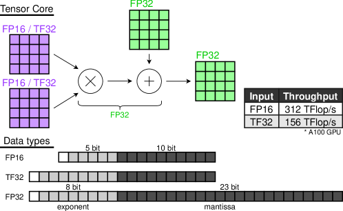
Figure 1: The input, output, and computation precision of Tensor Cores we use.

NVIDIA Tensor Cores are mixed-precision computing units for fixed-size matrix multiplications and additions on NVIDIA GPUs. When computing a large matrix multiplication on Tensor Cores, we split the input matrices and sum up the resulting matrices. The data type of input matrices to Tensor Cores is limited to low-precision, FP16, TF32, etc. Although the multiplication and addition are performed in high-precision, such as FP32, as shown in Fig. 1, the accuracy degrades when computing a single-precision GEMM on Tensor Cores since the input matrices have to be converted to low-precision. Our previous work (TCEC-SGEMM method) recovers this accuracy through compensated summation and the avoidance of rounding inside Tensor Cores, RZ (Round to Zero) [34]. We have demonstrated that the method can outperform the FP32 SIMT Core peak performance while the accuracy is at the same level as single-precision. In our method, the single-precision matrix multiplication $\mathbf{C}_{\text{F32}}\leftarrow\mathbf{A}_{\text{F32}}\cdot\mathbf{B}_{\text{F32}}$ is approximately computed as follows:

$$\mathbf{A}_{\text{low}} \leftarrow\text{toLow}\left(\mathbf{A}_{\text{F32}}\right)$$ (6)

$$\Delta\mathbf{A}_{\text{low}} \leftarrow\text{toLow}\left(\left(\mathbf{A}_{\text{F32}}-\text{toF32}\left(\mathbf{A}_{\text{low}}\right)\right)\times 2^{11}\right)$$ (7)

$$\mathbf{B}_{\text{low}} \leftarrow\text{toLow}\left(\mathbf{B}_{\text{F32}}\right)$$ (8)

$$\Delta\mathbf{B}_{\text{low}} \leftarrow\text{toLow}\left(\left(\mathbf{B}_{\text{F32}}-\text{toF32}\left(\mathbf{B}_{\text{low}}\right)\right)\times 2^{11}\right)$$ (9)

$$\mathbf{C}_{\text{F32}} \sim\mathbf{A}_{\text{low}}\cdot\mathbf{B}_{\text{low}}+(\Delta\mathbf{A}_{\text{low}}\cdot\mathbf{B}_{\text{low}}+\mathbf{A}_{\text{low}}\cdot\Delta\mathbf{B}_{\text{low}})\times 2^{-11},$$ (10)

where toLow converts an FP32 matrix to low-precision, FP16 or TF32, and toF32 converts a low-precision matrix to FP32. Since the matrix multiplications in Eq. (10) are computed on Tensor Cores in high precision, this method manages to compute the matrix multiplication in single precision. And we compute parts of additions inside $\mathbf{A}_{\text{low}}\cdot\mathbf{B}_{\text{low}}$ in Eq. (10) on FP32 SIMT Cores to use Round to Nearest (RN) for the rounding. We denote a Tensor Core which takes FP16 matrices as “FP16 Tensor Core” and one which takes TF32 matrices as “TF32 Tensor Core”.

3 Random projection by low-precision Gaussian random matrix

3.1 Floating point value representation of a Gaussian random value

The theoretical error bound of the random projection by Halko et al., Eq. (4), is proved mathematically under the implicit assumption that the Gaussian random value $g\in\mathcal{N}(0,1)$ has infinite precision. On the other hand, we represent $g$ as a floating point value format eXmY, which has X bit of exponent and Y bit of mantissa, and denote it as $g_{\text{eXmY}}$. For instance, FP32 is e8m23 and FP16 is e5m10. Furthermore, we use RN for the rounding, which is used by default in many modern processors, including NVIDIA GPUs. Due to the rounding error, the relation between $g$ and $g_{\text{eXmY}}$ is as follows.

$$g_{\text{eXmY}}=g+\Delta g$$ (11)

where $\Delta g$ is the rounding error. In the case of RN, the following inequality is satisfied.

$$-\text{exp\_of}(g_{\text{eXmY}})\times u_{Y}\leq\Delta g\leq\text{exp\_of}(g_{\text{eXmY}})\times u_{Y},$$ (12)

where $\text{exp\_of}(\cdot)$ is the exponent of the floating point value and $u_{Y}=2^{-(Y+1)}$.

3.2 Properties of low-precision Gaussian random value

The property of Gaussian random values represented in floating point varies among its formats. We examine the following three properties.

1. The overflow and underflow probability.

2. The number of elements within a specific range of the Gaussian distribution.

3. The mean and variance.

format	$p^{\text{of}}_{\tt eXmY}$	$p^{\text{not-normalized}}_{\tt eXmY}$	$p^{\text{uf}}_{\tt eXmY}$
FP8_1 (e4m3)	$\ll 2-2\Phi(2^{3})$ $<1\times 10^{-12}$	$6\times 10^{-3}$	$8\times 10^{-4}$
FP8_2 (e5m2)		$2\times 10^{-5}$	$6\times 10^{-6}$
FP16 (e5m10)		$2\times 10^{-5}$	$2\times 10^{-8}$
bfloat (e8m7)		$\ll 2\Phi(2^{-45})-1$ $<2\times 10^{-12}$
TF32 (e8m10)
FP32 (e8m23)
	$N^{1\sigma}_{\text{\tt eXmY}}$	$N^{2\sigma}_{\text{\tt eXmY}}$	$N^{4\sigma}_{\text{\tt eXmY}}$
FP8_1 (e4m3)	111	127	143
FP8_2 (e5m2)	119	127	135
FP16 (e5m10)	30,719	32,767	34,815
bfloat (e8m7)	32,511	32,767	33,023
TF32 (e8m10)	260,095	262,143	264,191
FP32 (e8m23)	2,130,706,431	2,147,483,647	2,164,260,863

Table 1: The properties of Gaussian random values represented in floating point values eXmY. Top: $p_{\text{eXmY}}^{\text{of}},p_{\text{eXmY}}^{\text{uf}}$ and $p_{\text{eXmY}}^{\text{not-normalized}}$ are the probabilities of overflow, underflow, and being denormalized values or underflowed, respectively. Bottom: The number of floating point values within $\sigma$, $2\sigma$, and $4\sigma$ ranges.

3.2.1 The overflow and underflow probability

If a Gaussian random value overflows with non-negligible probability, we can not compute the random projection correctly. On the other hand, it can be computed even if the underflow occurs with high probability since this is just a sparse random matrix [26]. We investigate these probabilities theoretically.

The maximum positive value $\text{max}_{\text{eXmY}}$ that can be represented as eXmY is calculated as follows:

$$\text{max}_{\text{eXmY}} =0b0^{\prime}{\underbrace{11\cdots 10}_{\text{X bit}}}^{\prime}\underbrace{11\cdots 1}_{\text{Y bit}}$$ (13)

$$=2^{2^{X}-2-\text{bias}(X)}\times\left(1-2^{-(Y+1)}\right)$$ (14)

$$=2^{2^{X-1}-1}\times\left(1-2^{-(Y+1)}\right),$$ (15)

where $\text{bias}(X)=2^{X-1}-1$ is the exponent bias of eXmY. Therefore, the overflow probability $p_{\text{eXmY}}^{\text{of}}$, in other words, the probability that a value larger than $\text{max}_{\text{eXmY}}$ appears is calculated as follows:

$$p_{\text{eXmY}}^{\text{of}}=2\times\left(1-\Phi(\text{max}_{\text{eXmY}})\right)$$ (16)

where $\Phi(\cdot)$ is the probability density function of the Gaussian distribution $\mathcal{N}(0,1)$. On the other hand, the minimum positive values $\text{min}_{\text{eXmY}}^{\text{normalized}}$ and $\text{min}_{\text{eXmY}}^{\text{denormalized}}$ that can be represented as a normalized and denormalized value of eXmY respectively are calculated as follows:

$$\text{min}_{\text{eXmY}}^{\text{normalized}} =0b0^{\prime}{\underbrace{00\cdots 01}_{\text{X bit}}}^{\prime}\underbrace{00\cdots 0}_{\text{Y bit}}$$

$$=2^{1-\text{bias}(X)}=2^{2-2^{X-1}}$$

$$\text{min}_{\text{eXmY}}^{\text{denormalized}} =0b0^{\prime}{\underbrace{00\cdots 00}_{\text{X bit}}}^{\prime}\underbrace{00\cdots 01}_{\text{Y bit}}$$

$$=2^{-\text{bias}(X)}\times 2^{-Y}=2^{1-2^{X-1}}\times 2^{-Y}.$$

Thus, the underflow probability $p_{\text{eXmY}}^{\text{uf}}$ and denormalized probability $p_{\text{eXmY}}^{\text{not-normalized}}$ are calculated as follows:

$$p_{\text{eXmY}}^{\text{uf}} =2\times(\Phi(\text{min}_{\text{eXmY}}^{\text{denormalized}})-1/2)$$

$$p_{\text{eXmY}}^{\text{not-normalized}} =2\times(\Phi(\text{min}_{\text{eXmY}}^{\text{normalized}})-1/2).$$

We show concrete values of $p_{\text{eXmY}}^{\text{of}},p_{\text{eXmY}}^{\text{uf}}$ and $p_{\text{eXmY}}^{\text{not-normalized}}$ for some floating point formats in the top of Table 1. Since the number of elements in a random matrix for random projection is typical up to $\sim 10^{8}$ ($n<10^{5},p<10^{3}$), the overflow probability is negligible when the exponent length X is larger than 3.

3.2.2 The number of elements within $2^{s}\sigma$ range

If the number of elements within a specific range of the Gaussian distribution is too small, the Gaussian random matrix might not have full rank, albeit with a very low probability, which is assumed in the proof of Eq. (4). As an extreme example, if only one value can appear, the rank of the random matrix is 0 or 1. We investigate the number of elements within the $2^{s}\sigma$ range of the Gaussian distribution.

A positive normalized number element $v_{\text{eXmY}}$ within $2^{s}\sigma$ range of the Gaussian distribution $\mathcal{N}(0,\sigma=1)$ satisfies the following inequality:

$$\text{min}_{\text{eXmY}}^{\text{normalized}}\leq v_{\text{eXmY}}<0b0^{\prime}{\underbrace{**\cdots**}_{=s+\text{bias}(X)}}^{\prime}\underbrace{00\cdots 0}_{\text{Y bit}}.$$ (17)

Therefore, the number of normalized number elements $N_{\text{eXmY}}^{2^{s}}$ within $2^{s}\sigma$ including 0 is calculated as follows:

$$N_{\text{eXmY}}^{2^{s}\sigma} =2\times(s+\text{bias}(X)+1)\times 2^{Y}+1.$$ (18)

We show the concrete values of $N_{\text{eXmY}}^{2^{s}}$ for some floating point formats at the bottom of Table 1. Although the number of elements in low-precision formats, such as FP16, is fewer than one in FP32, it is still larger than the existing sparse random projection methods, typically 3.

3.2.3 The mean and variance

When using RN for rounding, the mean of $g_{\text{eXmY}}$ is $0$ since the floating point value is symmetric with respect to the sign. On the other hand, the variance $\alpha_{Y}=\mathbb{E}_{g}({g_{\text{eXmY}}}^{2})-(\mathbb{E}_{g}(g_{\text{eXmY}}))^{2}=\mathbb{E}_{g}({g_{\text{eXmY}}}^{2})$, where $\mathbb{E}_{x}(y)$ is the mean of $y$ for $x$, is not $1$ even if the value generated with $\mathcal{N}(0,1)$ and rounded.

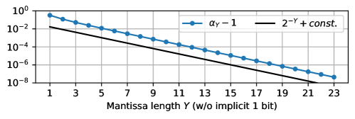
Figure 2: The variance of the Gaussian distribution represented in eXmY.

The variance $\alpha_{Y}$ is calculated as follows:

$$\alpha_{Y} =\mathbb{E}_{g}({g_{\text{eXmY}}}^{2})$$

$$=\sum_{v\in\text{eXmY}}v^{2}\left(\Phi(v+\text{exp\_of}(v)u_{Y})-\Phi(v-\text{exp\_of}(v))u_{Y}\right)$$

While this equation can not be calculated analytically, we perform a numerical computation, as shown in Fig. 2. The variance exponentially approaches $1$ for the mantissa length $Y$.

While Eq. (4) is the error bound when using $\mathcal{N}(0,1)$, we show the bound can be applied for any variance $\alpha$ as long as it is not too small. The proof of Eq. (4) comes as a proof of the following equation:

$$\mathbb{E}||\mathbf{\Sigma}_{2}\mathbf{G}_{2}\mathbf{G}_{1}^{\dagger}||_{F}^{2}=k/(p-1)\cdot||\mathbf{\Sigma}_{2}||^{2}_{F},$$ (19)

where $\Sigma_{2}$ is $\text{diag}(\sigma_{p+1},\cdots,\sigma_{k})$, $\mathbf{G}_{1},\mathbf{G}_{2}$ are $k\times k$ and $k\times(k-p)$ Gaussian random matrices respectively, and $\cdot^{\dagger}$ is a pseudo inverse of a matrix. This equation can be proven by following two theorems in [20] under the assumption that a Gaussian random matrix has full rank.

Theorem 2

For any matrix $\mathbf{S}\in\mathbb{C}^{n_{1}\times n_{2}},\mathbf{T}\in\mathbb{C}^{n_{3}\times n_{4}}$ and a $\mathcal{N}(0,1)$-Gaussian matrix $\mathbf{G}\in\mathbb{C}^{n_{2}\times n_{3}}$,

$$\mathbb{E}||\mathbf{S}\mathbf{G}\mathbf{T}||_{F}^{2}=||\mathbf{S}||_{F}^{2}||\mathbf{T}||_{F}^{2}.$$ (20)

Theorem 3

For a $\mathcal{N}(0,1)$-Gaussian random matrix $\mathbf{G}\in\mathbb{C}^{k\times(k+p)}$,

$$\mathbb{E}||\mathbf{G}^{\dagger}||_{F}^{2}=k/(p-1).$$ (21)

From these theorems, Eq. (19) is proved as follows.

$$\mathbb{E}_{\mathbf{G}_{1},\mathbf{G}_{2}}||\mathbf{\Sigma}_{2}\mathbf{G}_{2}\mathbf{G}_{1}^{\dagger}||_{F}^{2} =\mathbb{E}_{\mathbf{G}_{1}}\left(\mathbb{E}_{\mathbf{G}_{2}}\big{[}||\mathbf{\Sigma}_{2}\mathbf{G}_{2}\mathbf{G}_{1}^{\dagger}||_{F}^{2}\big{\rvert}\mathbf{\mathbf{G}_{1}}\big{]}\right)$$ (22)

$$=\mathbb{E}_{\mathbf{G}_{1}}\left(||\mathbf{\Sigma}_{2}||_{F}^{2}||\mathbf{G}_{1}^{\dagger}||_{F}^{2}\right) \because\text{Theorem \ref{thm:sgt}}$$ (23)

$$=||\mathbf{\Sigma}_{2}||_{F}^{2}\cdot\mathbb{E}_{\mathbf{G}_{1}}||\mathbf{G}_{1}^{\dagger}||_{F}^{2}$$ (24)

$$=k/(p-1)\cdot||\mathbf{\Sigma}_{2}||_{F}^{2}, \because\text{Theorem \ref{thm:g-inv}}$$ (25)

where $\mathbb{E}[X|Y]$ is a conditional expectation of $X$ given $Y$.

$\square$

To show that Eq. (4) is also true when using $\mathcal{N}(0,\alpha)$, it suffices to show Eq. (19) is true for any variance $\alpha$. Theorem 2 and Theorem 3 are extended as follows.

Theorem 4 (Extension of Theorem 2)

For any matrix $\mathbf{S}\in\mathbb{C}^{n_{1}\times n_{2}},\mathbf{T}\in\mathbb{C}^{n_{3}\times n_{4}}$ and a $\mathcal{N}(0,\alpha)$-Gaussian matrix $\mathbf{G}_{\alpha}\in\mathbb{C}^{n_{2}\times n_{3}}$,

$$\mathbb{E}||\mathbf{S}\mathbf{G}_{\alpha}\mathbf{T}||_{F}^{2}=\alpha||\mathbf{S}||_{F}^{2}||\mathbf{T}||_{F}^{2}.$$ (26)

Theorem 5 (Extension of Theorem 3)

For a $\mathcal{N}(0,\alpha)$-Gaussian random matrix $\mathbf{G}_{\alpha}\in\mathbb{C}^{k\times(k+p)}$,

$$\mathbb{E}||{\mathbf{G}_{\alpha}}^{\dagger}||_{F}^{2}=k/(p-1)\cdot\alpha^{-1}.$$ (27)

We apply these theorems in Eq. (22-25) and obtain the same equation as Eq. (19).

$\square$

Proof of Theorem 4. For $\mathbf{M}:=\mathbf{SGT}$ and $\mathbf{M}_{\alpha}:=\mathbf{S}\mathbf{G}_{\alpha}\mathbf{T}$, it suffices to show $\mathbb{E}|{\mathbf{M}_{\alpha}}_{(i,j)}|^{2}=\alpha\mathbb{E}|\mathbf{M}_{(i,j)}|^{2}$, where $\cdot_{(i,j)}$ is the $(i,j)$ element of the matrix. The elements $\mathbf{M}_{(i,j)}$ and ${\mathbf{M}_{\alpha}}_{(i,j)}$ are calculated as follows:

$$\mathbf{M}_{(i,j)} =\sum_{l_{a}}\sum_{l_{b}}\mathbf{S}_{(i,l_{a})}{\mathbf{G}}_{(l_{a},l_{b})}\mathbf{T}_{(l_{b},j)}$$

$${\mathbf{M}_{\alpha}}_{(i,j)} =\sum_{l_{a}}\sum_{l_{b}}\mathbf{S}_{(i,l_{a})}{\mathbf{G}_{\alpha}}_{(l_{a},l_{b})}\mathbf{T}_{(l_{b},j)}.$$

Therefore, $\mathbb{E}|\mathbf{M}_{(i,j)}|^{2}$ and $\mathbb{E}|{\mathbf{M}_{\alpha}}_{(i,j)}|^{2}$ are calculated as follows:

$$\mathbb{E}|\mathbf{M}_{(i,j)}|^{2}$$

$$=\sum_{l_{a},l_{a^{\prime}},l_{b},l_{b^{\prime}}}|\mathbf{S}_{(i,l_{a})}\mathbf{S}_{(i,l_{a^{\prime}})}\mathbf{T}_{(l_{b},j)}\mathbf{T}_{(l_{b^{\prime}},j)}|\times\mathbb{E}\left({\mathbf{G}}_{(l_{a},l_{b})}{\mathbf{G}}_{(l_{a^{\prime}},l_{b^{\prime}})}\right)$$ (28)

$$=\sum_{l_{a}}\sum_{l_{b}}|\mathbf{S}_{(i,l_{a})}|^{2}\cdot|\mathbf{T}_{(l_{b},j)}|^{2},$$ (29)

$$\mathbb{E}|{\mathbf{M}_{\alpha}}_{(i,j)}|^{2}$$

$$=\sum_{l_{a},l_{a^{\prime}},l_{b},l_{b^{\prime}}}|\mathbf{S}_{(i,l_{a})}\mathbf{S}_{(i,l_{a^{\prime}})}\mathbf{T}_{(l_{b},j)}\mathbf{T}_{(l_{b^{\prime}},j)}|\times\mathbb{E}\left({\mathbf{G}_{\alpha}}_{(l_{a},l_{b})}{\mathbf{G}_{\alpha}}_{(l_{a^{\prime}},l_{b^{\prime}})}\right)$$ (30)

$$=\alpha\sum_{l_{a}}\sum_{l_{b}}|\mathbf{S}_{(i,l_{a})}|^{2}\cdot|\mathbf{T}_{(l_{b},j)}|^{2}=\alpha\mathbb{E}|\mathbf{M}_{(i,j)}|^{2}.$$ (31)

We use the following facts for obtaining Eq. (29) and (31), respectively, that are led from the definition of variance and the product of two values from independent distributions.

$$\mathbb{E}\left(\mathbf{G}_{(i_{1},j_{1})}\mathbf{G}_{(i_{2},j_{2})}\right) =\left\{\begin{array}[]{ll}1&(i_{1}=i_{2}\text{\&}j_{1}=j_{2})\\ 0&\text{otherwise}\end{array}\right.$$ (34)

$$\mathbb{E}\left({\mathbf{G}_{\alpha}}_{(i_{1},j_{1})}{\mathbf{G}_{\alpha}}_{(i_{2},j_{2})}\right) =\left\{\begin{array}[]{ll}\alpha&(i_{1}=i_{2}\text{\&}j_{1}=j_{2})\\ 0&\text{otherwise}\end{array}\right.$$ (37)

$\square$

Proof of Theorem 5. For a Gaussian random matrix $\mathbf{G}\in\mathbb{R}^{m\times n}$, $(\mathbf{GG}^{\top})^{-1}$ follows an inverse Wishart distribution [1]. The mean of the inverse Wishart distribution is calculated as follows:

$$\mathbb{E}((\mathbf{GG}^{\top})^{-1})=1/(n-m-1)\cdot\mathbf{S}_{\mathbf{G}}^{-1},$$ (38)

where $\mathbf{S}_{\mathbf{G}}$ is the covariance matrix of $\mathbf{G}$. Since $||\mathbf{G}^{{\dagger}}||_{F}^{2}=\text{tr}[(\mathbf{G}^{\dagger})^{\top}\mathbf{G}^{\dagger}]=\text{tr}[(\mathbf{GG}^{\top})^{-1}]$,

$$\mathbb{E}||\mathbb{\mathbf{G}^{\dagger}}||_{F}^{2}=1/(n-m-1)\cdot\text{tr}[\mathbf{S}_{\mathbf{G}}^{-1}].$$ (39)

When $\mathbf{G}$ is a $k\times(k-p)$ matrix $\mathbf{G}_{r}^{\text{Y}}$, the off-diagonal elements of $\mathbf{S}_{\mathbf{GG}}^{\top}$ are zeros and diagonal elements are $\alpha$. Therefore, we obtain the following equation:

$$\mathbb{E}||\mathbb{\mathbf{G}^{\dagger}}||_{F}^{2}=k/(p-1)\cdot\alpha^{-1}.$$ (40)

$\square$

3.3 Numerical experiment

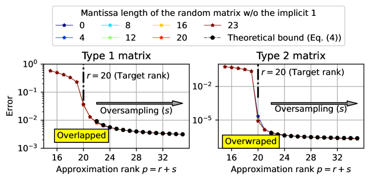
Figure 3: The accuracy of the random projection using low-precision Gaussian matrices for two kinds of input matrices. The error is calculated as $||\mathbf{A}-\mathbf{Q}\mathbf{Q}^{\top}\mathbf{A}||_{F}$.

We conduct a numerical experiment to investigate the effect of the mantissa length on the accuracy of the random projection. The FP32 input matrices $\mathbf{A}_{t1}$ and $\mathbf{A}_{t2}$ are generated in two ways that are used in the numerical experiment of [9] as follows.

• Type 1: For $\mathbf{D}=\text{diag}(\mathbf{I}_{r},0)\in\mathbb{R}^{n\times n}$, we define

  $$\mathbf{A}_{t1}=\mathbf{D}+(\xi/\epsilon)\mathbf{GG}^{\top},$$

  where $\mathbf{G}$ is a Gaussian random matrix. We fix $\xi=10^{-4},n=4096$ and $r=20$.

• Type 2: For orthogonal random matrices $\mathbf{U},\mathbf{V}\in\mathbf{R}^{n\times n}$ in the Haar distribution, and

  $$\mathbf{D}=\text{diag}(\phi\mathbf{I},2^{-\alpha},3^{-\alpha},\cdots,(n-r+1)^{-\alpha}),$$

  we define $\mathbf{A}_{t2}=\mathbf{U}\mathbf{D}\mathbf{V}^{\top}$. We fix $n=4096,r=20,\alpha=3$ and $\phi=10^{6}$.

The Gaussian random matrix $\mathbf{G}$ is generated in FP32 and rounded to low mantissa length values by RN. To avoid the effect of the rounding error, we convert both the input matrices and random matrices to FP64 and compute the random projection in FP64. The evaluation result is shown in Fig. 3. In both test matrices, the accuracy of the random projection is almost the same across all mantissa lengths.

3.4 Combination with existing sparse random projection methods

The existing sparse random projection method uses a sparse random matrix generated by Eq. (5). When computing the random projection using the sparse random matrix $\mathbf{\Omega}$, we do not need to multiply $\sqrt{n}$ in Eq. (5) since we only use the orthonormal matrix of the projected matrix. Therefore, we can use a sparse random matrix where each element is one of $\{-1,0,1\}$ for the random projection. These values can be represented even if the mantissa has only the implicit 1 bit. Thus, the mixed-precision random projection method can also be applied to (very) sparse random matrix methods with the same accuracy. However, we only focus on the Gaussian random projection in the rest of this paper since it is the best-understood class of the random matrices in RandNLA theoretically [20].

4 Single and half-precision matrix multiplication on Tensor Cores

4.1 Algorithm

We can compute a multiplication of single-precision matrix $\mathbf{A}_{\text{F32}}$ and half-precision matrix $\mathbf{B}_{\text{F16}}$ in single-precision accuracy by just omitting a term in TCEC-SGEMM emulation method as follows:

$$\mathbf{A}_{\text{low}} \leftarrow\text{toLow}\left(\mathbf{A}_{\text{F32}}\right)$$ (41)

$$\Delta\mathbf{A}_{\text{low}} \leftarrow\text{toLow}\left(\left(\mathbf{A}_{\text{F32}}-\text{toF32}\left(\mathbf{A}_{\text{low}}\right)\right)\times 2^{11}\right)$$ (42)

$$\mathbf{B}_{\text{low}} \leftarrow\text{toLow}\left(\mathbf{B}_{\text{F16}}\right)$$ (43)

$$\mathbf{C}_{\text{SH}} \sim\mathbf{A}_{\text{low}}\cdot\mathbf{B}_{\text{low}}+\Delta\mathbf{A}_{\text{low}}\cdot\mathbf{B}_{\text{low}}\times 2^{-11}.$$ (44)

Since the computational complexity of this method is $2/3$ of TCEC-SGEMM, it can compute the matrix multiplication faster when the matrix $\mathbf{B}_{\text{F32}}$ can be expressed by FP16. We call this method SHGEMM (Single- and Half-precision GEMM).

4.2 Implementation

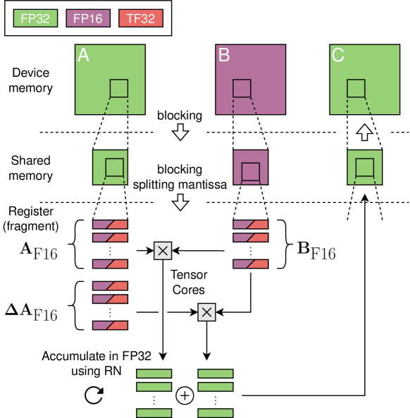
Figure 4: The computing flow of SHGEMM on Tensor Cores in our implementation.

We implement the SHGEMM kernel function from scratch using WMMA API and WMMA API extension library [35]. When using FP16 Tensor Cores, the supported exponent range of $\mathbf{A}_{\text{F32}}$ is limited to that of FP16. Therefore, we implement two kinds of SGEMM: 1) limited exponent range SHGEMM using FP16 Tensor Cores (SHGEMM-FP16), and 2) full exponent range supporting SHGEMM using TF32 Tensor Cores (SHGEMM-TF32). Since the theoretical peak performance of FP16 Tensor Cores is $2\times$ higher than TF32 Tensor Cores, SHGEMM-FP16 is theoretically faster than SHGEMM-TF32. Even for the implementation of SHGEMM-TF32, the matrix $\mathbf{B}_{\text{F16}}$ is stored in FP16 on device memory, loaded and stored in FP16 on shared memory, and converted to TF32 on registers before input to Tensor Cores, as shown in Fig. 4. The implementation is available on GitHub.

4.3 Rounding error analysis

We analyze the rounding error bound of SHGEMM briefly and show that it is the same as the computation on FP32 SIMT Cores. We use the mma.m16n8k8 PTX instruction which computes a matrix multiplication and addition on Tensor Cores. It suffices to analyze the error bound of an inner product $c=\mathbf{x}^{\top}\mathbf{y}=\Sigma_{i=1}^{n}x_{i}y_{i}$. The properties of the computation using the PTX instruction and the avoidance of RZ are as follows:

• One instruction accumulates eight resulting values of the multiplication.

• The mantissa length of the accumulator inside Tensor Cores is 25-bit, including the implicit bit.

• A multiplication of two 11-bit mantissa values is conducted without rounding error and accumulated with RZ.

• The accumulated eight values are rounded by RZ and output in FP32.

• The accumulation of the resulting values of eight values is conducted on FP32 SIMT Cores with RN.

These properties have been confirmed theoretically or empirically through small numerical experiments. The inner product is split into the accumulation of the eight elements accumulation as follows:

$$c=\sum_{i=1}^{n^{\prime}}t_{i}\text{ \ \ \ for \ \ \ }t_{i}=\sum_{j=1+8(i-1)}^{8i}x_{j}y_{j},$$

where $n^{\prime}=n/8$. First, we obtain the rounding error bound of an inner product of two FP16 vectors. We define $\tilde{c}$ and $\tilde{t}_{i}$ as the results of computing $c$ and $t_{i}$ on Tensor Cores, respectively, as follows:

$$\tilde{c}=\text{fl}_{RX}\left(\sum_{i=1}^{n^{\prime}}\text{RZ}_{F32}\left(\tilde{t}_{i}\right)\right),\text{ \ \ }\tilde{t}_{i}=\text{fl}_{tc}\left(\sum_{j=1+8(i-1)}^{8i}x_{j}y_{j}\right),$$

where $\text{fl}_{RX}(f)$ denotes the computations of $f$ with RX for the rounding to be either RN or RZ. $\text{fl}_{tc}(f)$ is on Tensor Cores, which have the properties above, and $\text{RZ}_{F32}(\cdot)$ is a rounding function from 25-bit mantissa to FP32 by RZ. In $\text{fl}_{RX}(f)$, the bound of rounding error is as follows:

$$\text{RX}(a)=a(1+\delta),|\delta|\leq\hat{u}\equiv\left\{\begin{array}[]{ll}u&\text{RX is RN}\\ 2u&\text{RX is RZ},\end{array}\right.$$ (47)

where $u$ is the unit round off of FP32 and $2^{-24}$. The RZ mode is the default mode on Tensor Cores, and the RN mode is used in SHGEMM, as same as TCEC-SGEMM. Furthermore, the rounding error of $\tilde{t}_{i}$ are bounded as follows:

$$\tilde{t}_{i}=t_{i}+\Delta_{i}\text{ \ s.t. \ }|\Delta_{i}|\leq\underbrace{7}_{\text{Num additions}}\cdot\underbrace{2u^{\prime}}_{\text{RZ}}\cdot\left(\sum_{j=1+8(i-1)}^{8i}|x_{j}y_{j}|\right),$$

where $u^{\prime}=2^{-25}$. Then, the following rounding error equation is satisfied.

$$\tilde{c}=\sum_{i=1}^{n^{\prime}}\text{RZ}_{F32}(\tilde{t}_{i})+\Delta=\sum_{i=1}^{n^{\prime}}(t_{i}+\Delta_{i})(1+\delta_{i})+\Delta$$

where $\delta_{i}$ is $\delta$ for $\tilde{t}_{i}$ in Eq. (47) and $\Delta$ is a value that satifies $|\Delta|\leq(n^{\prime}-1)\hat{u}\sum_{i=1}^{n^{\prime}}\text{RZ}_{F32}(\tilde{t}_{i})$. We obtain the error bound of the inner product as follows by expanding inequalities of $\delta_{i}$, $\Delta_{i}$, and $\Delta$.

$$|\tilde{c}-c|=\left|\tilde{c}-\sum_{i=1}^{n^{\prime}}t_{i}\right|\lesssim\left|\sum_{i=1}^{n^{\prime}}(t_{i}\delta_{i}+\Delta_{i}(1+\delta_{1}))+\Delta\right|\lesssim\frac{1}{8}n\hat{u}|x^{\top}||y|,$$

where $|x^{\top}||y|$ is the inner product of elementwise absolute value vectors of $x$ and $y$. Then, we extend the analysis of the rounding error of the inner product to a multiplication of two FP16 matrices in FP32, $\mathbf{A}_{\text{F16}}\cdot\mathbf{B}_{\text{F16}}$, and obtain its error bound inequalities as follows:

$$|\tilde{\mathbf{C}}-\mathbf{A}_{\text{F16}}\cdot\mathbf{B}_{\text{F16}}|\lesssim\left\{\begin{array}[]{ll}\frac{1}{8}nu|\mathbf{A}_{\text{F16}}||\mathbf{B}_{\text{F16}}|&\text{RX is RN}\\ \frac{1}{4}nu|\mathbf{A}_{\text{F16}}||\mathbf{B}_{\text{F16}}|&\text{RX is RZ},\end{array}\right.$$ (50)

for $n\geq 8$, where $\tilde{\mathbf{C}}$ is the computation result and $|\cdot|$ is the element-wise absolute value.

Next, we obtain the error bound of SHGEMM using the error bound of Tensor Cores and avoidance of RZ above. In Eq. (41-42), the matrix $\mathbf{A}_{\text{F32}}$ is split into three terms as follows:

$$\mathbf{A}_{\text{F32}}=\mathbf{A}_{\text{F16}}+\Delta\mathbf{A}_{\text{F16}}+\mathbf{A}_{\Delta},$$ (51)

where $\mathbf{A}_{\Delta}$ is the loss of mantissa caused by the splitting, where its expected length is 0.25-bit [34]. For the split matrices, the following inequalities are satisfied:

$$|\mathbf{A}_{\text{F16}}|\leq(1+u_{\text{F16}})|\mathbf{A}_{\text{F32}}|,|\Delta\mathbf{A}_{\text{F16}}|\leq u_{\text{F16}}|\mathbf{A}_{\text{F32}}|,|\mathbf{A}_{\mathbf{\Delta}}|\leq u_{\text{F16}}^{2}|\mathbf{A}_{\text{F32}}|,$$ (52)

where $u_{\text{F16}}$ is the unit round off of FP16 and $2^{-11}$. We compute the SHGEMM as follows:

$$\tilde{\mathbf{C}}_{\text{SH}} =\text{fl}\left(\mathbf{A}_{\text{F16}}\mathbf{B}_{\text{F16}}+\Delta\mathbf{A}_{\text{F16}}\mathbf{B}_{\text{F16}}\right)$$ (53)

$$=\mathbf{A}_{\text{F16}}\mathbf{B}_{\text{F16}}+\mathbf{\Delta}^{(1)}+\Delta\mathbf{A}_{\text{F16}}\mathbf{B}_{\text{F16}}+\mathbf{\Delta}^{(2)}$$

$$+\delta(\mathbf{A}_{\text{F16}}\mathbf{B}_{\text{F16}}+\mathbf{\Delta}^{(1)}+\Delta\mathbf{A}_{\text{F16}}\mathbf{B}_{\text{F16}}+\mathbf{\Delta}^{(2)}),$$ (54)

where $\mathbf{\Delta}^{(1)}$ and $\mathbf{\Delta}^{(2)}$ are the rounding error in $\mathbf{A}_{\text{F16}}\mathbf{B}_{\text{F16}}$ and $\Delta\mathbf{A}_{\text{F16}}\mathbf{B}_{\text{F16}}$, respectively. We use Oomoto’s RZ avoiding method for computing $\mathbf{A}_{\text{F16}}\mathbf{B}_{\text{F16}}$, but not for $\Delta\mathbf{A}_{\text{F16}}\mathbf{B}_{\text{F16}}$. Therefore, the following inequalities are satisfied by Eq. (50) and (52):

$$|\mathbf{\Delta}^{(1)}| \lesssim\frac{1}{8}nu|\mathbf{A}_{\text{F32}}||\mathbf{B}_{\text{F16}}|$$ (55)

$$|\mathbf{\Delta}^{(2)}| \lesssim\frac{1}{4}nuu_{\text{F16}}|\mathbf{A}_{\text{F32}}||\mathbf{B}_{\text{F16}}|.$$ (56)

Thus, we obtain the following inequality on the rounding error bound of SHGEMM by expanding Eq. (54):

$$|\tilde{\mathbf{C}}_{\text{SH}}-\mathbf{A}_{\text{F32}}\cdot\mathbf{B}_{\text{F16}}|\lesssim\frac{1}{8}nu|\mathbf{A}_{\text{F32}}||\mathbf{B}_{\text{F16}}|,$$ (57)

for $n\geq 8$. When computing the multiplication $\mathbf{A}_{\text{F32}}\cdot\mathbf{B}_{\text{F16}}$ all on FP32 SIMT Cores with 8 elements blocking similarly, the primary bounding term is also $\frac{1}{8}nu|\mathbf{A}_{\text{F32}}||\mathbf{B}_{\text{F16}}|$. Therefore, the error bound of SHGEMM is the same as the computation on FP32 SIMT Cores.

4.4 Evaluation of SHGEMM

All numerical experiments are conducted on NVIDIA A100 SXM4 (40GB) GPU and AMD EPYC 7702 CPU.

4.4.1 Accuracy

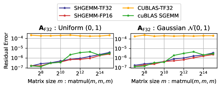
Figure 5: The accuracy of matrix multiplication $\mathbf{A}_{\text{F32}}\cdot\mathbf{B}_{\text{F16}}$ on SHGEMM. The matrix $\mathbf{B}_{\text{F16}}$ is generated with a Gaussian distribution $\mathcal{N}(0,1)$ and $\mathbf{A}_{\text{F32}}$ is $\mathcal{N}(0,1)$ (right) or a uniform distribution $(0,1)$ (left).

The accuracy of the SHGEMM implementation is shown in Fig. 5. We compute the multiplication $\mathbf{A}_{\text{F32}}\cdot\mathbf{B}_{\text{F16}}$, where $\mathbf{A}_{\text{F32}}$ is initialized with $\mathcal{N}(0,1)$ or a uniform distribution $(0,1)$, and $\mathbf{B}_{\text{F16}}$ is $\mathcal{N}(0,1)$. We also compare the accuracy of cuBLAS SGEMM and cuBLAS TF32 GEMM by converting the matrix $\mathbf{B}_{\text{F16}}$ to FP32. The relative error is calculated as follows:

$$\mathrm{RelativeError}=||\mathbf{C}_{\text{SH}}-\mathbf{C}_{\text{F64}}||_{F}/||\mathbf{C}_{\text{F64}}||_{F},$$

where $\mathbf{C}_{\text{F64}}$ is computed in FP64 by converting the input matrices to FP64. The accuracy of the SHGEMM implementations is at the same level as cuBLAS SGEMM.

4.4.2 Throughput

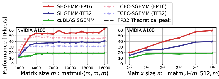
Figure 6: Left: The throughput comparison of cuBLAS SGEMM, TCEC-SGEMM, and SHGEMM. The suffixes FP16 and TF32 denote the Tensor Core type used in the GEMM implementation. Right: The throughput comparison of SHGEMM for tall-skinny matrix multiplication used in rank-$512$ Randomized SVD for $m\times m$ matrix.

The throughput of the SHGEMM implementation is shown in Fig. 6. The throughput is calculated as $2mnk/t$ [Flop/s] for matmul-($m,n,k$), which computes the multiplication of $m\times k$ and $k\times n$ matrices, and $t$ is the computing time [sec]. We compare the throughput of the two SHGEMM implementations, TCEC-SGEMM implementations that use FP16 Tensor Cores and TF32 Tensor Cores, and cuBLAS SGEMM. The achieved throughput of SHGEMM-FP16 is up to $61.0$ [TFlop/s], and SHGEMM-TF32 is $40.5$ [TFlop/s]. Each SHGEMM implementation is faster than TCEC-SGEMM, which uses the same Tensor Cores.

The theoretical peak performance of SHGEMM-FP16 and SHGEMM-TF32 on NVIDIA A100 GPU are $312/2=156$ [TFlop/s] and $152/2=76$ [TFlop/s], respectively, under the following assumption.

Assumption 1

All computations on computing units other than Tensor Cores can be overlapped with the ones on Tensor Cores. In other words, the Tensor Core instruction is issued every clock cycle.

Therefore, the efficiency of SHGEMM-FP16 is only $39$%, and SHGEMM-TF32 is $53$%, respectively. As the cause of the low efficiency, we consider it difficult to realize the Assumption 1 for the following reasons.

1. There is a dependency in the order of Tensor Cores and FP32 SIMT Cores computations in Eq. (41-44). Therefore, these computations can not be overlapped.

2. The computing time on FP32 SIMT Cores for computing Eq. (42) and avoiding RZ inside Tensor Cores is large. When splitting the resulting matrix of matmul($m,n,k$) into a grid where each matrix size is $b_{m}\times b_{n}$, and computing the result for each sub-divided matrices in parallel, the number of loaded $\mathbf{A}_{\text{F32}}$ elements is $mnk/b_{n}$. Therefore, the number of subtractions and multiplications in Eq. (42) is $2mnk/b_{n}$, computed on FP32 SIMT Cores. Furthermore, we use FP32 SIMT Cores for accumulating the result of multiplications of sub-divided matrices to avoid RZ inside Tensor Cores $2mnk/f_{k}$ times, where $f_{k}$ is the $k$ value of the matmul that one Tensor Core instruction computes, which is $8$. On the other hand, the number of calculations on Tensor Cores in Eq. (44) is $4mnk$. Thus, the computation ratio on FP32 SIMT Cores and Tensor Cores is $(2/b_{n}+1/f_{k}):4$ independent from $m,n$, and $k$. The ratio is about $1:25$ since we set $b_{n}=64$ or $128$ typically. Therefore, the computing time on FP32 SIMT Cores is not negligible against the one on Tensor Cores since the theoretical throughput ratio of FP32 SIMT Cores and Tensor Cores is only $1:16$ on FP16 Tensor Cores and $1:8$ on TF32 Tensor Cores.

5 Experiments

5.1 Randomized SVD

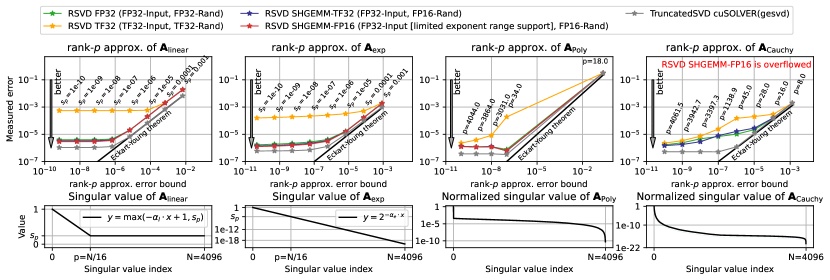
Figure 7: Top: The accuracy of Randomized SVD implementations for the input matrices $\mathbf{A}_{\text{linear}},\mathbf{A}_{\text{exp}}$ and $\mathbf{A}_{\text{Cauchy}}$. Bottom: The singular value decay of input matrices and target ranks.

We use SHGEMM in line 1 of Algorithm 1 and NVIDIA cuBLAS and cuSOLVER libraries for the other part of the computations of the algorithm.

5.1.1 Accuracy

For the evaluation of accuracy, we use 4 kinds of test matrices as follows:

• $\mathbf{A}_{\text{linear}}$ and $\mathbf{A}_{\mathrm{exp}}\in\text{FP32}^{4096\times 4096}$: First, we decide a value $s_{p}\in(0,1)$ and generate a FP32 value sequence $\{s_{j}\}$ as follows.

  • For $\mathbf{A}_{\text{linear}}$: $s_{i}=\text{max}\left(-\alpha_{l}\times i+1,s_{p}\right)$ where $\alpha_{l}=(1-s_{p})/p$.

  • For $\mathbf{A}_{\text{exp}}$: $s_{i}=2^{-\alpha_{e}\times i}$ where $\alpha_{e}=(\log_{2}1/s_{p})/p$.

  Then, we use the LAPACK slatms function to make a $N\times N$ FP32 random matrix with $s_{i}$ as singular values. By generating the matrix in this way, we can calculate the error bound of $p$-rank approximation using Theorem 1. Therefore, the error bound of relative residual of $p$-rank approximation for $\mathbf{A}_{\text{linear}}$ is

  $$s_{p}\sqrt{N-p}/||\mathbf{A}_{\text{linear}}||_{F}$$

  and for $\mathbf{A}_{\text{exp}}$ is

  $$\sqrt{(s_{p}^{2}-2^{2qN})/(1-2^{2q})}/||\mathbf{A}_{\text{exp}}||_{F}.$$

  In this evaluation, $N$ and $p$ are fixed to $4096$ and $256$. By fixing these parameters, we fix the computational complexity of Randomized SVD. Thus, the rounding error accumulation is also fixed to some extent, and we can compare the effect of the accuracy of random projection for the approximation accuracy.

• $\mathbf{A}_{\text{Poly}}\in\text{FP32}^{4096\times 4096}$: The generation equation is the same as the matrix type 2 in 3.3. We used the parameters $r=20,\alpha=3$ and $\phi=10^{6}$.

• $\mathbf{A}_{\text{Cauchy}}\in\text{FP32}^{4096\times 4096}$: We generate Cauchy matrices as follows and apply orthogonal iteration 1 time.

  $${\mathbf{A}_{\text{Cauchy}}}_{i,j}=1/\left(|x_{i}-y_{i}|+\gamma\right),$$

  where $x_{i},y_{i}$ are random sequences in $(-10^{-3},10^{-3})$ and $\gamma=10^{-3}$. The absolute value of some elements of this matrix exceeds the representation range of the FP16. Therefore, the computation is expected to fail when using SHGEMM-FP16.

We fix the oversampling parameter $s=10$ and evaluate ten matrices generated using different random seeds. We compare the accuracy of the Randomized SVD across the GEMM implementations as shown in Fig. 5. The data type of the random matrix is FP16 when using SHGEMM, otherwise FP32. The accuracy of RSVD TF32 degrades compared to RSVD FP32, which is the baseline, since the accuracy of TF32 GEMM is worse than SGEMM. This implies that it is critical to preserve the accuracy of the input matrix during the random projection. On the other hand, the accuracy of RSVD SHGEMM-TF32 and SHGEMM-FP16 are at the same level as RSVD FP32.

5.1.2 Throughput

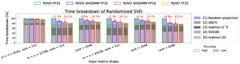
Figure 8: The time breakdown of baseline Randomized SVD (FP32) on NVIDIA A100 and computing time reduction by our method. The prefix numbers of the breakdown labels are the line numbers in Algorithm 1.

The throughput comparison of the Randomized SVD implementations is shown in Fig. 8. Although the asymptotic computational complexity of the random projection is larger than SVD and QR decomposition, their real computing times are not negligible. Therefore, in the case of $m=n=8192,rank=512$, we can not speed up the whole computation since their computing time consumes about 90% of the whole. On the other hand, we have reduced up to 18.9 % and 22.1% of the whole computing time using SHGEMM-TF32 and SHGEMM-FP16, respectively, while the accuracy is at the same level as FP32 when the computing time ratios of SVD and QR decomposition are not too large.

5.2 Random Projection HOSVD

We evaluate the effect of our method for High-Order Singular Value Decomposition (HOSVD) [11]. The HOSVD factorizes an $N$-dimension tensor $\mathbf{A}\in\mathbb{R}^{I_{1}\times I_{2}\times\cdots\times I_{N}}$ into multiplications of an $N$-dimensional tensor and matrices as follows:

$$\mathbf{A}=\mathbf{g}\times_{1}\mathbf{Q}_{1}^{\top}\times_{2}\mathbf{Q}_{2}^{\top}\cdots\times_{N}\mathbf{Q}_{N}^{\top},$$ (58)

where $\mathbf{g}\in\mathbb{R}^{J_{1}\times J_{2}\times\cdots\times J_{N}}$ is a core tensor and $\mathbf{Q}_{k}\in\mathbb{R}^{I_{k}\times J_{k}}$ is an orthogonal matrix. We denote the contraction of a tensor $\mathbf{T}\in\mathbb{R}^{I_{1}\times I_{2}\times\cdots\times I_{N}}$ and a matrix $\mathbf{M}\in\mathbb{R}^{I_{i}\times k}$ at $i$-th mode as $\mathbf{T}\times_{i}\mathbf{M}$. The rank in each dimension determines the shape of the core tensor. HOSVD is computed by flattening to matrix and SVD. The random projection HOSVD (RP-HOSVD) [3] shown in Algorithm 2 computes this factorization using random projection and QR factorization instead of SVD.

Algorithm 2 Random projection HOSVD

1:Input matrix $\mathbf{A}\in\mathbb{R}^{I_{1}\times I_{2}\times\cdots\times I_{N}}$, Target rank $r\in\mathbb{N}$

2:$\mathbf{g}\in\mathbb{R}^{J_{1}\times J_{2}\times\cdots\times J_{N}},\mathbf{Q}_{k}\in\mathbb{R}^{I_{k}\times J_{k}}$   s.t. $\mathbf{A}\sim\mathbf{g}\times_{1}\mathbf{Q}_{1}\times_{2}\mathbf{Q}_{2}\cdots\times_{N}\mathbf{Q}_{N}$

3:for $\ \textbf{do}\text{ \ }i=1..N$

4:     $\mathbf{W}\leftarrow\mathbf{A}_{(i)}^{\prime}\cdot\mathbf{\Omega}_{(i)}$ where $\mathbf{A}_{(i)}^{\prime}\in\mathbb{R}^{I_{i}\times\left(\Pi_{k\neq i}I_{k}\right)}$ is a transposed matrix of the tensor $\mathbf{A}$, and $\mathbf{\Omega}_{(i)}\in\mathbb{R}^{\left(\Pi_{k\neq i}I_{k}\right)\times J_{i}}$ is a random matrix.

5:     $\mathbf{Q}_{i},\_\leftarrow\text{QR}\left(\mathbf{W}\right)$

6:end for

7:$\mathbf{g}\leftarrow\mathbf{A}\times_{1}\mathbf{Q}^{\top}_{1}\times_{2}\mathbf{Q}^{\top}_{2}\cdots\times_{N}\mathbf{Q}^{\top}_{N}$

To evaluate RP-HOSVD, we generate test tensors as in Algorithm 3 and measure the approximation accuracy and throughput, as shown in Fig. 9. As with the Randomized SVD accuracy, the accuracy degrades when we use TF32 random projection. On the other hand, when using SHGEMM-TF32 and SHGEMM-FP16 random projection, we have reduced the computing times by 36.6% and 43.0%, respectively. Although the accuracy of RP-HOSVD by SHGEMM is better than the FP32 baseline in some cases, we consider that the cause is the difference in the computation order, which is also shown in the unit test of SHGEMM in Fig. 5. Therefore, we conclude that the accuracy of RP-HOSVD by SHGEMM is almost at the same level as FP32.

Algorithm 3 Tensor generation for RP-HOSVD evaluation

Input tensor dims ${I_{i}\in\mathbb{N}}$, Target ranks $J_{i}\in\mathbb{N}$, Rank padding $p\in\mathbb{N}$

Input tensor $\mathbf{A}\in\mathbb{R}^{I_{1}\times I_{2}\times\cdots\times I_{N}}$

$\mathbf{G}\leftarrow$ GenRand($-1,1$) $\in\mathbb{R}^{J_{1}\times J_{2}\times\cdots\times J_{N}}$

for $\ \textbf{do}i=1..N$

     $\mathbf{\Omega}_{\alpha}\leftarrow$ GenRand($-1,1$) $\in\mathbb{R}^{J_{i}\times(J_{i}-p)}$

     $\mathbf{\Omega}_{\beta}\leftarrow$ GenRand($-1,1$) $\in\mathbb{R}^{(J_{i}-p)\times I_{i}}$

     $\mathbf{\Omega}_{(i)}\leftarrow\mathbf{\Omega}_{\alpha}\cdot\mathbf{\Omega}_{\beta}$ // This is a ($J_{i}-p$)-rank matrix

     $\mathbf{G}\leftarrow\mathbf{G}\times_{i}\mathbf{\Omega}_{(i)}$

end for

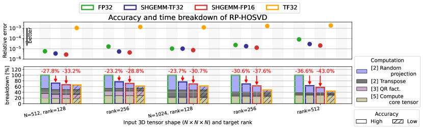
Figure 9: The accuracy (top) and time breakdown (bottom) of random projection HOSVD on NVIDIA A100. The prefix numbers of the breakdown labels are the line numbers in Algorithm 2.

6 Conclusion

We propose a fast mixed-precision random projection method for single-precision tensors leveraging the high throughput of Tensor Cores while maintaining approximation accuracy. We confirm the property of low-precision Gaussian random values for the random projection. The matrix multiplication for the random projection, SHGEMM, achieves $61.0$ TFlop/s using FP16 Tensor Cores and $40.5$ TFlop/s using TF32 Tensor Cores. Using this method, we improve the throughput of Randomized SVD by $1.28$ times and Random projection HOSVD by $1.75$ times compared to baseline FP32 implementations while maintaining accuracy.

Acknowledgements

The authors would like to thank Professor Katsuhisa Ozaki for technical assistance and discussion. This work was supported by JSPS KAKENHI Grant Numbers JP20K20624, JP22H03598, and JP21J14694. This work is supported by ”Joint Usage/Research Center for Interdisciplinary Large-scale Information Infrastructures” in Japan (Project ID: jh220022-NAH, jh220009-NAHI).

References

- [1] Aspects of Multivariate Statistical Theory. Wiley Series in Probability and Statistics, Hoboken, NJ, USA, March 1982. John Wiley & Sons, Inc.
- [2] Dimitris Achlioptas. Database-friendly random projections: Johnson-Lindenstrauss with binary coins. Journal of Computer and System Sciences, 66(4):671–687, 2003.
- [3] Salman Ahmadi-Asl, Stanislav Abukhovich, Maame G. Asante-Mensah, Andrzej Cichocki, Anh Huy Phan, Tohishisa Tanaka, and Ivan Oseledets. Randomized Algorithms for Computation of Tucker Decomposition and Higher Order SVD (HOSVD). IEEE Access, 9:28684–28706, 2021. Conference Name: IEEE Access.
- [4] AMD. AMD CDNA™ 2 ARCHITECTURE, 2021.
- [5] Ashima Anand and Amit Kumar Singh. Cloud based secure watermarking using IWT-Schur-RSVD with fuzzy inference system for smart healthcare applications. Sustainable Cities and Society, 75:103398, December 2021.
- [6] Maolin Che, Yimin Wei, and Hong Yan. Randomized algorithms for the low multilinear rank approximations of tensors. Journal of Computational and Applied Mathematics, 390:113380, 2021.
- [7] Chuangquan Chen, Chi-Man Vong, Chi-Man Wong, Weiru Wang, and Pak-Kin Wong. Efficient extreme learning machine via very sparse random projection. Soft Computing, 22(11):3563–3574, June 2018.
- [8] Chung-Cheng Chiu, James Qin, Yu Zhang, Jiahui Yu, and Yonghui Wu. Self-supervised learning with random-projection quantizer for speech recognition. In Proceedings of the 39th International Conference on Machine Learning, pages 3915–3924. PMLR, June 2022. ISSN: 2640-3498.
- [9] Michael P. Connolly, Nicholas J. Higham, and Srikara Pranesh. Randomized Low Rank Matrix Approximation: Rounding Error Analysis and a Mixed Precision Algorithm, July 2022. Issue: 2022.10 Number: 2022.10.
- [10] NVIDIA Corporation. NVIDIA A100 TENSOR CORE GPU, 2020.
- [11] Lieven De Lathauwer, Bart De Moor, and Joos Vandewalle. A Multilinear Singular Value Decomposition. SIAM Journal on Matrix Analysis and Applications, 21(4):1253–1278, January 2000. Publisher: Society for Industrial and Applied Mathematics.
- [12] Petros Drineas and Michael W. Mahoney. RandNLA: randomized numerical linear algebra. Communications of the ACM, 59(6):80–90, 2016.
- [13] Carl Eckart and Gale Young. The approximation of one matrix by another of lower rank. Psychometrika, 1(3):211–218, September 1936.
- [14] N. Benjamin Erichson, Steven L. Brunton, and J. Nathan Kutz. Compressed Singular Value Decomposition for Image and Video Processing. In 2017 IEEE International Conference on Computer Vision Workshops (ICCVW), pages 1880–1888, October 2017. ISSN: 2473-9944.
- [15] N. Benjamin Erichson, Lionel Mathelin, J. Nathan Kutz, and Steven L. Brunton. Randomized Dynamic Mode Decomposition. SIAM Journal on Applied Dynamical Systems, 18(4):1867–1891, 2019. Publisher: Society for Industrial and Applied Mathematics.
- [16] Xu Feng, Wenjian Yu, and Yaohang Li. Faster Matrix Completion Using Randomized SVD. In 2018 IEEE 30th International Conference on Tools with Artificial Intelligence (ICTAI), pages 608–615, January 2018. ISSN: 2375-0197.
- [17] Xiaoli Zhang Fern and Carla E. Brodley. Random projection for high dimensional data clustering: a cluster ensemble approach. In Proceedings of the Twentieth International Conference on International Conference on Machine Learning, ICML’03, pages 186–193, Washington, DC, USA, 2003. AAAI Press.
- [18] Dmitriy Fradkin and David Madigan. Experiments with random projections for machine learning. In Proceedings of the ninth ACM SIGKDD international conference on Knowledge discovery and data mining, KDD ’03, pages 517–522, New York, NY, USA, 2003. Association for Computing Machinery.
- [19] Ming Gu and Stanley C. Eisenstat. Efficient Algorithms for Computing a Strong Rank-Revealing QR Factorization. SIAM Journal on Scientific Computing, February 2012. Publisher: Society for Industrial and Applied Mathematics.
- [20] N. Halko, P. G. Martinsson, and J. A. Tropp. Finding Structure with Randomness: Probabilistic Algorithms for Constructing Approximate Matrix Decompositions. SIAM Review, 53(2):217–288, 2011. Publisher: Society for Industrial and Applied Mathematics.
- [21] Chinmay Hegde, Michael Wakin, and Richard Baraniuk. Random Projections for Manifold Learning. In Advances in Neural Information Processing Systems, volume 20. Curran Associates, Inc., 2007.
- [22] Siriwan Intawichai and Saifon Chaturantabut. A Missing Data Reconstruction Method Using an Accelerated Least-Squares Approximation with Randomized SVD. Algorithms, 15(6):190, June 2022. Number: 6 Publisher: Multidisciplinary Digital Publishing Institute.
- [23] Norman P. Jouppi, Cliff Young, Nishant Patil, and et al. In-Datacenter Performance Analysis of a Tensor Processing Unit. In Proceedings of the 44th Annual International Symposium on Computer Architecture, ISCA ’17, pages 1–12, New York, NY, USA, June 2017. Association for Computing Machinery.
- [24] Saehoon Kim and Seungjin Choi. Bilinear Random Projections for Locality-Sensitive Binary Codes. pages 1338–1346, 2015.
- [25] Mu Li, Wei Bi, James T. Kwok, and Bao-Liang Lu. Large-Scale Nyström Kernel Matrix Approximation Using Randomized SVD. IEEE Transactions on Neural Networks and Learning Systems, 26(1):152–164, January 2015. Conference Name: IEEE Transactions on Neural Networks and Learning Systems.
- [26] Ping Li, Trevor J. Hastie, and Kenneth W. Church. Very sparse random projections. In Proceedings of the 12th ACM SIGKDD international conference on Knowledge discovery and data mining, KDD ’06, pages 287–296, New York, NY, USA, 2006. Association for Computing Machinery.
- [27] Junichiro Makino. Present, Past and Future. In Junichiro Makino, editor, Principles of High-Performance Processor Design: For High Performance Computing, Deep Neural Networks and Data Science, pages 147–155. Springer International Publishing, Cham, 2021.
- [28] Stefano Markidis, Steven Wei Der Chien, Erwin Laure, Ivy Bo Peng, and Jeffrey S. Vetter. NVIDIA Tensor Core Programmability, Performance & Precision. 2018 IEEE International Parallel and Distributed Processing Symposium Workshops (IPDPSW), pages 522–531, May 2018. arXiv: 1803.04014.
- [29] Brendan McCane. Random projections for feature matching. In Proceedings of the 29th International Conference on Image and Vision Computing New Zealand, IVCNZ ’14, pages 78–83, New York, NY, USA, 2014. Association for Computing Machinery.
- [30] Vineetha Menon, Qian Du, and James E. Fowler. Fast SVD With Random Hadamard Projection for Hyperspectral Dimensionality Reduction. IEEE Geoscience and Remote Sensing Letters, 13(9):1275–1279, September 2016. Conference Name: IEEE Geoscience and Remote Sensing Letters.
- [31] Rachel Minster, Arvind K. Saibaba, and Misha E. Kilmer. Randomized Algorithms for Low-Rank Tensor Decompositions in the Tucker Format. SIAM Journal on Mathematics of Data Science, 2(1):189–215, 2020. Publisher: Society for Industrial and Applied Mathematics.
- [32] Daichi Mukunoki, Katsuhisa Ozaki, Takeshi Ogita, and Toshiyuki Imamura. DGEMM Using Tensor Cores, and Its Accurate and Reproducible Versions. In Ponnuswamy Sadayappan, Bradford L. Chamberlain, Guido Juckeland, and Hatem Ltaief, editors, High Performance Computing, Lecture Notes in Computer Science, pages 230–248, Cham, 2020. Springer International Publishing.
- [33] Mahmoud Nabil. Random Projection and Its Applications, October 2017. Number: arXiv:1710.03163 arXiv:1710.03163 [cs].
- [34] Hiroyuki Ootomo and Rio Yokota. Recovering single precision accuracy from Tensor Cores while surpassing the FP32 theoretical peak performance:. The International Journal of High Performance Computing Applications, June 2022. Publisher: SAGE PublicationsSage UK: London, England.
- [35] Hiroyuki Ootomo and Rio Yokota. Reducing shared memory footprint to leverage high throughput on Tensor Cores and its flexible API extension library. In Proceedings of the International Conference on High Performance Computing in Asia-Pacific Region, HPC Asia ’23, pages 1–8, New York, NY, USA, February 2023. Association for Computing Machinery.
- [36] Katsuhisa Ozaki, Takeshi Ogita, Shin’ichi Oishi, and Siegfried M. Rump. Error-free transformations of matrix multiplication by using fast routines of matrix multiplication and its applications. Numerical Algorithms, 59(1):95–118, January 2012.
- [37] Fabian Pedregosa, Gaël Varoquaux, Alexandre Gramfort, Vincent Michel, Bertrand Thirion, Olivier Grisel, Mathieu Blondel, Peter Prettenhofer, Ron Weiss, Vincent Dubourg, Jake Vanderplas, Alexandre Passos, David Cournapeau, Matthieu Brucher, Matthieu Perrot, and Édouard Duchesnay. Scikit-learn: Machine Learning in Python. Journal of Machine Learning Research, 12(85):2825–2830, 2011.
- [38] Vladimir Rokhlin and Mark Tygert. A fast randomized algorithm for overdetermined linear least-squares regression. Proceedings of the National Academy of Sciences, 105(36):13212–13217, September 2008. Publisher: Proceedings of the National Academy of Sciences.
- [39] Gil Shabat, Yaniv Shmueli, Yariv Aizenbud, and Amir Averbuch. Randomized LU decomposition. Applied and Computational Harmonic Analysis, 44(2):246–272, March 2018.
- [40] O. P. Singh, Amit Kumar Singh, Amrit Kumar Agrawal, and Huiyu Zhou. SecDH: Security of COVID-19 images based on data hiding with PCA. Computer Communications, 191:368–377, July 2022.
- [41] Grigorios Tsagkatakis and Andreas Savakis. Random Projections for face detection under resource constraints. In 2009 16th IEEE International Conference on Image Processing (ICIP), pages 1233–1236, January 2009. ISSN: 2381-8549.
- [42] Nguyen Xuan Vinh, Sarah Erfani, Sakrapee Paisitkriangkrai, James Bailey, Christopher Leckie, and Kotagiri Ramamohanarao. Training robust models using Random Projection. In 2016 23rd International Conference on Pattern Recognition (ICPR), pages 531–536, February 2016.
- [43] Han Wang and James Anderson. Large-Scale System Identification Using a Randomized SVD. In 2022 American Control Conference (ACC), pages 2178–2185, June 2022. ISSN: 2378-5861.
- [44] Mingrui Yang, Dan Ma, Yun Jiang, Jesse Hamilton, Nicole Seiberlich, Mark A. Griswold, and Debra McGivney. Low rank approximation methods for MR fingerprinting with large scale dictionaries. Magnetic Resonance in Medicine, 79(4):2392–2400, 2018. _eprint: https://onlinelibrary.wiley.com/doi/pdf/10.1002/mrm.26867.
- [45] Jiani Zhang, Jennifer Erway, Xiaofei Hu, Qiang Zhang, and Robert Plemmons. Randomized SVD methods in hyperspectral imaging. Journal of Electrical and Computer Engineering, 2012:3:3, 2012.
- [46] Jingyi Zhang, Ping Ma, Wenxuan Zhong, and Cheng Meng. Projection-based techniques for high-dimensional optimal transport problems. WIREs Computational Statistics, page e1587.