Inner Approximations of Stochastic Programs for Data-driven Stochastic Barrier Function Design

Abstract

This paper proposes a new framework to compute finite-horizon safety guarantees for discrete-time piece-wise affine systems with stochastic noise of unknown distributions. The approach is based on a novel approach to synthesise a stochastic barrier function (SBF) from noisy data and rely on the scenario optimization theory. In particular, we show that the stochastic program to synthesize a SBF can be relaxed into a chance-constrained optimisation problem on which scenario approach theory applies. We further show that the resulting program can be reduced to a linear programming problem, thus guaranteeing efficiency. In contrast to existing approaches, this method is data efficient as it only requires the number of data to be proportional to the logarithm in the negative inverse of the confidence level and is computationally efficient due to its reduction to linear programming. The efficacy of the method is empirically evaluated on various verification benchmarks. Experiments show a significant improvement with respect to state-of-the-art, obtaining tighter certificates with a confidence that is several orders of magnitude higher.

I Introduction

The behavior of modern autonomous systems are often uncertain, due to e.g., sensor noise or unknown dynamics, and are commonly employed in safety-critical applications, such as automated driving [1] or robotics [2]. These applications require formal guarantees of safety in order for the system to be deployed in real-life. Consequently, computing such guarantees for stochastic systems represents an important, but non-trivial, area of research [3]. Existing approaches to address this problem either rely on abstractions, where the original system is abstracted into a finite state model, generally a variant of a Markov chain [4], or leverage the concept of Stochastic Barrier Functions (SBFs) [5]. SBFs are Lyapunov-like functions that can be employed to bound the probability that a dynamical system will remain safe for a given time horizon, without the need to explicitly evolve the system over time. A common assumption for the vast majority of the existing approaches is that the distribution of the system is known, and often either Gaussian or of bounded support [5, 6]. Unfortunately, in practice, the noise characteristics of the system are generally not known [7, 8]. This leads to the main question of this paper: how can we compute formal certificates of safety for stochastic systems with unknown noise distribution?

This paper focuses on guaranteeing safety for stochastic piece-wise affine (PWA) systems. In particular, a data-driven framework for the design of SBFs for stochastic PWA systems with unknown noise distribution is presented. By relying on tools from probability theory and convex optimisation, we show that the problem of synthesising a SBF for this class of systems can be reformulated as a chance-constrained optimisation problem [9]. This reformulation allows employing the scenario approach theory to devise a data-driven framework to synthesize SBFs with high confidence. The resulting approach is data-efficient, as it only requires the amount of data to be logarithmic in the negative inverse of the confidence, and is scalable, as, in the case of PWA SBFs, it reduces to the solution of a Linear Programming (LP) problem. We experimentally evaluate the performance of the method on various systems including a model of a vehicle in windy conditions. Our analysis illustrates how our approach outperforms state-of-the-art comparable methods both in terms of tightness of bounds and amount of data required to achieve the desired confidence. In summary, the main contributions are:

• A data-driven method based on the scenario approach to design piece-wise affine Stochastic Barrier Functions.

• A novel inner chance-constrained approximation to stochastic programming.

• Empirical studies that illustrates the performance of the proposed method compared to state-of-the-art in terms of both certified safety probability and confidence.

The structure of the paper is as follows: Section II reviews convex and scenario optimisation, which are used extensively throughout the paper. Section III describes the safety certification problem and Section IV how SBFs formally can guarantee safety. In Section V are the main results of this paper; namely the inner approximation to stochastic programming and data-driven SBF design. Empirical studies are reported in Section VI.

Related works

SBFs were first proposed in [10] to study the probability that a stochastic system exits a given set in a finite time using super-martingale theory. Since then, various works have employed SBFs to study non-linear stochastic systems with approaches including sum-of-squares (SoS) optimisation [5, 6, 11, 12, 13] and relaxations to convex programming [14, 15]. However, all these methods assume that the model of the system is fully known. A recent set of works have started to study data-driven approaches to design SBFs for stochastic systems with (partially) unknown dynamics, which can be employed to obtain guarantees of safety with a confidence [16, 12]. These approaches replace the stochastic program for synthesising SBFs with a Sample Average Approximation (SAA)-based program, meaning that the expectation is replaced by the sample average with a probabilistic guarantee of satisfaction of the original expectation constraint through concentration inequalities. However, these methods require an amount of data that is proportional to the negative inverse of the confidence. In contrast, our approach requires a number of data that is logarithmic in the negative inverse of the confidence.

Data-driven verification of stochastic systems is a relatively new area to address the problem of verifying (partially) unknown systems [17, 18, 19, 20, 16, 12]. To compute formal guarantees for non-linear systems, apart from the SAA approach described in the previous paragraph, existing literature focuses either on the scenario approach [18, 19, 20], on Gaussian processes [21, 22], or on distributionally robust approaches [7]. In particular, in [18, 19, 20] the authors rely on the data efficiency of scenario approach theory to build abstractions of the original system with high confidence of correctness, while in [21, 22] error bounds on performing Gaussian Process regression are employed to again build abstractions that are employed to perform probabilistic model checking of the unknown system. However, all these methods are abstraction-based. Consequently, they suffer from the scalability issues inherent with abstraction-based frameworks. In this paper, our approach will combine the data-efficiency of the scenario approach with the flexibility of SBFs.

I-A Notation

The set of real, non-negative real, and natural numbers are denoted with $\mathbb{R}$, $\mathbb{R}_{\geq 0}$, and $\mathbb{N}$ respectively. Vectors in the Euclidean space will be denoted by the letter $x\in\mathbb{R}^{n}$ and random variables in $\mathbb{R}^{n}$ will be denoted with bold font $\mathbf{x}$. Subscripts will be used to denote a collection of elements, i.e., $x_{1},\ldots,x_{m}$ denote different vectors in the same space. A subset $X$ of $\mathbb{R}^{n}$ is convex if $\lambda x_{1}+(1-\lambda)x_{2}\in X$, for all $x_{1},x_{2}\in X$ and $\lambda\in[0,1]$. A polyhedron $P\subseteq\mathbb{R}^{n}$ is a convex set defined as $P=\{x\in\mathbb{R}^{n}:Hx\leq h\},$ where the matrix $H\in\mathbb{R}^{m\times n}$ and the vector $h\in\mathbb{R}^{m}$ are given, and the inequality is interpreted element-wise. This form is called a half-space representation. A function $f:\mathbb{R}^{n}\mapsto\mathbb{R}$ is convex if and only if its epigraph $\operatorname{epi}(f)$, defined as $\operatorname{epi}(f)=\{(x,t)\in\mathbb{R}^{n+1}:f(x)\leq t\}$, is a convex set of $\mathbb{R}^{n+1}$. Optimisation variables will be denoted by the letter $z$ to distinguish it from the state-space variable $x$.

II Preliminaries

In this section, we review some concepts used extensively throughout the paper.

II-A Robust linear programming

Robust linear programming (LP) [23] forms a backbone in this paper, hence we will reiterate its definition and crucial results. Consider the following robust LP problem for polyhedron $P\subset\mathbb{R}^{n}$

$$\operatorname*{\min}_{z} \quad s^{\top}z$$ (1)

$$\operatorname{s.t.} \quad a(z)^{\top}x\leq b(z),\quad\text{ for all }x\in P$$

where $z\in\mathbb{R}^{d}$ is the decision variable, $s\in\mathbb{R}^{d}$ is the cost vector, and $a:\mathbb{R}^{d}\to\mathbb{R}^{n},b:\mathbb{R}^{d}\to\mathbb{R}$ are functions affine in $z$. The following result guarantees that Problem 1 can be reformulated as a LP problem in a lifted space.

Proposition 1 (Strong duality of robust LP [23])

Consider the robust LP problem in Problem (1) and the following optimisation problem

$$\operatorname*{\min}_{z,\lambda} \quad s^{\top}z$$ (2)

$$\operatorname{s.t.} \quad h^{\top}\lambda\leq b(z)$$

$$\quad H^{\top}\lambda=a(z),\quad\lambda\geq 0.$$

where $(H,h)$ is the half-space representation of $P$. Let sets

$$\mathcal{Z} =\{z\in\mathbb{R}^{d}:\sup_{x\in P}a(z)^{\top}x\leq b(z)\},$$

$$\mathcal{Z}^{\prime} =\{z\in\mathbb{R}^{d}:\exists\lambda\in\mathbb{R}^{m}_{\geq 0},~{}h^{\top}\lambda\leq b(z),~{}H^{\top}\lambda=a(z)\},$$

be the feasible set of Problem (1) and the feasible set of Problem (2) projected onto its first $d$ coordinates, respectively. Then we have that $\mathcal{Z}=\mathcal{Z}^{\prime}$.

II-B Scenario optimisation

The scenario approach theory establishes sample complexity guarantees for the probability of constraint violation of a chance-constrained optimisation problem [24]. Let $(\Omega,\mathcal{F},\mathbb{P})$ be a probability space, where $\Omega$ is the sample space, $\mathcal{F}$ is a $\sigma$-algebra over $\Omega$, and $\mathbb{P}$ is a probability measure over $\mathcal{F}$. Then, a chance-constrained program is defined as:

$$\min_{z} \quad s^{\top}z$$ (3)

$$\operatorname{s.t.} \quad\mathbb{P}\{\omega\in\Omega:g(z,\omega)\leq 0\}\geq 1-\epsilon,$$

where $z\in\mathbb{R}^{d}$ is the optimisation variable, $s\in\mathbb{R}^{d}$ are the cost coefficients, $g:\mathbb{R}^{d}\times\Omega\to\mathbb{R}$ is a function that is convex in $z$ for each value of $\omega$ and measurable in $\omega$ for each value of $z$, and $\epsilon\in(0,1)$ is a given bound on constraint violation.

Now assume ${D}=\{\omega_{1},\ldots,\omega_{N}$} is a set of independent samples from $\mathbb{P}$. Note that the set ${D}$ belongs to the space $(\Omega^{N},\otimes_{N}\mathcal{F},\mathbb{P}^{N})$, where $\Omega^{N}$ is the $N$-fold Cartesian product of $\Omega$, and $\otimes_{N}\mathcal{F}$ is the product $\sigma$-algebra generated by the $\sigma$-algebra $\mathcal{F}$ and $\mathbb{P}^{N}$ represents the induced measure on $\Omega^{N}$ [24]. Then, at the core of the scenario approach is the construction of the scenario program

$$\operatorname*{\min}_{z} \quad s^{\top}z$$ (4)

$$\operatorname{s.t.} \quad g(z,\omega)\leq 0,\quad\text{ for all }\omega\in{D}.$$

The idea of the scenario approach is to use Problem (4) to obtain high confidence bounds on the solution of Problem (3). To do that, we need some standard assumptions [24].

Assumption 1

Assume that:

• $\mathbb{P}^{N}$-almost surely, the feasible set of Problem (4) given by $\mathcal{Z}=\{z\in\mathbb{R}^{d}:g(z,\omega)\leq 0,\text{ for all }\omega\in{D}\},$ has non-empty interior.

• $\mathbb{P}^{N}$-almost surely, the optimal solution of Problem (4) exists and is unique.

Denote by $z^{\star}({D})$ the unique, optimal solution of Problem (4), which is a random variable from $\Omega^{N}$ to $\mathbb{R}^{d}$. Then, we are ready to state Proposition 2.

Proposition 2 ([24])

Let $N\in\mathbb{N}$ represent the number of available samples and $V(z)=\mathbb{P}\{\omega\in\Omega:g(z,\omega)>0\}.$ be the probability of constraint violation associated with $z^{\star}({D})$. Assume a threshold $\epsilon\in(0,1)$ is given. Then we have that

$$\mathbb{P}^{N}\{{D}\in\Omega^{N}:V(z^{\star}({D}))>\epsilon\}\leq\sum_{i=0}^{d-1}\binom{N}{i}\epsilon^{i}(1-\epsilon)^{N-i}.$$

Proposition 2 will be key in establishing safety guarantees for the class of stochastic models considered in this paper.

III Problem statement

The goal of this paper is to certify safety for piece-wise affine stochastic systems, which we formally introduce in Section III-A, while probabilistic safety is introduced in Section III-B.

III-A Piece-wise affine stochastic systems

Let ${\mathcal{P}}=\{{P}_{1},\ldots,{P}_{\ell}\}$ be a polyhedral partition of the state space $X\subseteq\mathbb{R}^{n}$, where each ${P}_{i}$, $i=1,\ldots,\ell$ is given by its half-space representation. Consider the following discrete-time stochastic PWA system:

$$\mathbf{x}(k+1)=f(\mathbf{x}(k))+\eta(k),\quad\mathbf{x}(0)\in{X_{0}},$$ (5)

where $k\in\mathbb{N}$ denotes the (discrete) time index, ${X_{0}}$ is a set of initial states, and $f:X\mapsto\mathbb{R}^{n}$ is a PWA vector field given by

$$f(x)=f_{i}(x)=A_{i}x+b_{i},\quad x\in{P}_{i}\subseteq\mathbb{R}^{n},$$

for some matrix $A_{i}\in\mathbb{R}^{n\times n}$ and vector $b_{i}\in\mathbb{R}^{n}$. The additive term $(\eta(k))_{k\in\mathbb{N}}$ is a sequence of independent and identically distributed random variables representing an additive noise term. We assume that $\eta(k)$ is defined on the filtered probability space $(\Omega,\mathcal{F},(\mathcal{F}_{k})_{k\in\mathbb{N}},\mathbb{P})$, where $\mathcal{F}_{k}$ is the natural filtration of the process $\eta(k)$, and $\mathbb{P}$ is assumed to be unknown. Consequently, $(\mathbf{x}(k))_{k\in\mathbb{N}}$ is also a stochastic process in the space $(\Omega,\mathcal{F},\mathbb{P})$ that is, it is $\mathcal{F}_{k-1}$-measurable [9]. We note that System (5) represents a flexible and expressive model. In fact, not only does it include linear systems, but we note that PWA functions can approximate any non-linear function arbitrarily well.

III-B Time-bounded probabilistic safety

Our goal is to study probabilistic safety for System (5).

Definition 1 (Probabilistic safety [5])

Let $T\in\mathbb{N}$ be a time horizon and ${\mathcal{S}}$ be a measurable subset of $X$. We define probability safety for System (5) as

$$\zeta({\mathcal{S}},T)=\mathbb{P}\{\omega\in\Omega:\mathbf{x}(k)\in{\mathcal{S}}\text{ for all }k\in\{0,\ldots,T\}\}.$$ (6)

We assume that, while $f$ is known, $\eta$ is unknown and we can only generate independent and identically distributed (iid.) samples from it. Under these assumptions, the goal in this paper is to compute a (non-trivial) lower bound on $\zeta({\mathcal{S}},T)$ for System (5).

Our approach is based on using the sampled data to synthesize a piece-wise affine (PWA)Stochastic Barrier Function (SBF)for System (5) with high confidence. In order to do that, in Section V-A we develop a novel and powerful inner approximation for the feasible set of stochastic programs in terms of chance-constrained optimisation. This result is employed to use the scenario approach to synthesize SBF for System (5) with high confidence and by requiring a number of data logarithmic in the negative inverse of the confidence. In Section V-B, we show that in the setting considered in this paper the resulting optimization problem reduces to LP, thus enabling efficient and scalable synthesis. Before presenting the main result, we review in the next section SBFs and how they can be employed to guarantee a lower bound on $\zeta({\mathcal{S}},T)$.

IV Stochastic barrier function (SBF)

SBFs are Lyapunov-like functions commonly employed to compute the safety probability of stochastic systems [5].

Definition 2 (Stochastic Barrier Function)

Let ${\mathcal{U}}=X\setminus{\mathcal{S}}$ be the unsafe set and ${X_{0}}\subseteq{\mathcal{S}}$ the set of initial states, then a non-negative function $B:X\mapsto\mathbb{R}_{\geq 0}$ is called a Stochastic Barrier Function if there exist non-negative constants $\gamma,{c}$ satisfying the following conditions

$$B(x)\leq\gamma, ~{}\text{ for all }x\in{X_{0}},$$ (7)

$$B(x)\geq 1, ~{}\text{ for all }x\in{\mathcal{U}},$$ (8)

$$\mathbb{E}\left[B(f(x)+\eta(\omega))\right]\leq B(x)+{c},~{}\text{ for all }x\in{\mathcal{S}}.$$ (9)

where the expectation is with respect to $\omega\sim\mathbb{P}$.

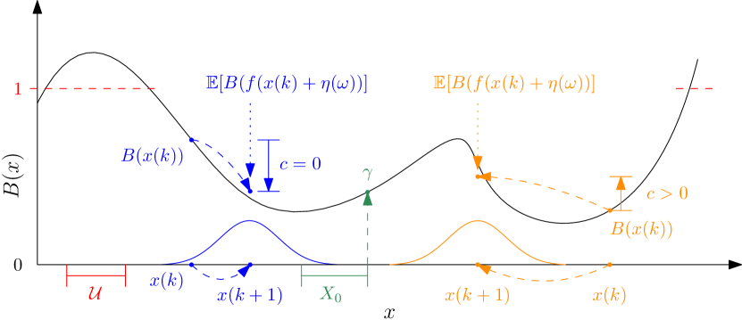
Figure 1: The figure is borrowed from [15]. A SBF $B(x)$ is a non-negative function that is greater than $1$ in an unsafe region ${\mathcal{U}}$, which is the complement of the safe set ${\mathcal{S}}$. The variable $\gamma$ is an upper bound for $B(x)$ over an initial region ${X_{0}}$. The upper bound for the expected increase in $B(x)$ after one step of (5) over the safe set ${\mathcal{S}}$ is denoted ${c}$. Then it holds that the probability of safety $\zeta({\mathcal{S}},T)\geq 1-(\gamma+{c}T)$.

A pictorial representation of a SBF is presented in Figure 1. Intuitively, the conditions in Definition 2 allows one to use martingale inequalities to lower bound probabilistic safety.

Proposition 3 ([10, Chapter 3, Theorem 3])

Let $B$ be a SBF satisfying the conditions in Definition 2 for System (5), time horizon $T$, and safe set ${\mathcal{S}}$. Then, it holds that $\zeta({\mathcal{S}},T)\geq 1-(\gamma+{c}T)$.

Thanks to Proposition 3, a sufficient condition to establish a lower bound on the safety probability is to design a SBF satisfying Equations (7)-(9). This can be obtained by solving the following stochastic program where $B$ is parameterised by $\theta$ as $B(x,\theta)$ according to a chosen function class

$$\min\limits_{\gamma,\,{c},\,\theta}\quad\gamma+{c}T,$$ (BP)

subject to the conditions in Definition 2. In other words, synthesis of a SBF can be framed as a minimisation over $\gamma+{c}T$. In this optimisation problem, the expectation condition (Equation (9)) can generally be computed analytically only under some strong assumptions on the noise distribution [25, 6]. Our approach proposes a new, inner chance-constrained approximation of Problem (BP), which allows us to rely on tools from scenario optimisation to synthesize a barrier [24]. The resulting approach is a distribution-free, data-driven method to obtain a SBF as a safety certificate with a high confidence of validity. Note that to guarantee the convexity of Problem (BP), $B$ is generally restricted to be either a SoS polynomial or an exponential function [6]. In this paper, motivated by the structure of System (5), we will consider piece-wise affine $B$, which have the flexibility to be able to model arbitrarily well any continuous function assuming the number of pieces of $B$ is large enough.

V Data-driven stochastic barrier function design

In this section, we present the main results of this paper. In Section V-A, an inner approximation of the feasible set of Problem (BP) in terms of a chance-constrained problem (Theorem 1) is described. Such a relaxation allows us to use the scenario approach to derive high confidence bounds on the resulting solution (Corollary 1). Finally in Section V-B, we will introduce PWA SBFs and show how for this class of barriers the resulting scenario approach is a LP.

V-A Data-driven stochastic barrier design

Solving Problem (BP) is challenging because analytic expressions of the expectation constraint are rarely available, even if the distribution $\mathbb{P}$ is known (which is not the case in this paper). To solve this problem, in Theorem 1, we derive a chance-constrained problem whose feasible set is a subset of the feasible set for Problem (BP). Thus, its optimal solution is an upper bound to that of Problem (BP).

Theorem 1

Consider System (5), and the barrier function $B(x,\theta)$ as in Definition 2, where $B$ is convex in $\theta$. Assume a given $\epsilon\in(0,1)$ and $M\geq 1$, and define decision variables $z=({c},\gamma,\theta)$. Let $g(x,z,\eta(\omega))=B(f(x)+\eta(\omega),\theta)$ and $h(x,z)=B(x,\theta)+{c}$, and choose ${\nu}\geq\frac{\epsilon M}{1-\epsilon}$. Define the set

$$E(x,z)=\left\{\omega\in\Omega:g(x,z,\eta(\omega))+{\nu}\leq h(x,z)\right\}.$$

Then, the feasible set of the chance-constrained barrier program

$$\min_{\gamma\geq 0,\,{c}\geq 0,\,\theta} \quad\gamma+{c}T$$ (CCBP)

$$\operatorname{s.t.} \quad\begin{aligned} &\begin{aligned} &B(x,\theta)\in[0,M],&&\quad\text{ for all }x\in\mathbb{R}^{n},\\[4.30554pt] &B(x,\theta)\leq\gamma,&&\quad\text{ for all }x\in{X_{0}},\\[4.30554pt] &B(x,\theta)\geq 1,&&\quad\text{ for all }x\in{\mathcal{U}},\\[4.30554pt] \end{aligned}\\ &\mathbb{P}\left\{E(x,z)\right\}\geq 1-\epsilon,\text{ for all }x\in{\mathcal{S}},\end{aligned}$$

is contained in the feasible set of Problem (BP).

The proof of Theorem 1 is reported in Section VIII. Theorem 1 opens new ways for data-driven design of Stochastic Barrier Functions. Rather than relying on standard concentration inequalities to approximate the expectation in Equation (9) as in [16], we can perform chance-constraint tightening with the parameter ${\nu}$ to guarantee the feasible set of (SBP) is an inner approximation of (CCBP). Building on this result, in Corollary 1 we use the scenario approach to design SBFs from data with high confidence.

Corollary 1

Assume that ${D}=\{\omega_{1},\ldots,\omega_{N}\}$ is a collection of $N$ independent samples from the distribution $\mathbb{P}$. Fix $\epsilon\in(0,1)$, $M\geq 1$ and ${\nu}\geq\frac{\epsilon M}{1-\epsilon}$, and let $\beta=\sum_{i=0}^{d-1}\binom{N}{i}\epsilon^{i}(1-\epsilon)^{N-i},$ where $d=|\theta|+2$. Let $({c}^{\star},\gamma^{\star},\theta^{\star})$ be the optimal solution to the scenario program

$$\min_{\gamma\geq 0,\,{c}\geq 0,\,\theta} \quad\gamma+{c}T$$ (SBP)

$$\operatorname{s.t.} \quad B(x,\theta)\in[0,M], \text{ for all }x\in\mathbb{R}^{n},$$

$$\quad B(x,\theta)\leq\gamma, \text{ for all }x\in{X_{0}},$$

$$\quad B(x,\theta)\geq 1, \text{ for all }x\in{\mathcal{U}},$$

$$\quad g(x,z,\eta(\omega))+{\nu}\leq h(x,z),$$

$$\qquad\text{ for all }\omega\in{D}, \text{ for all }x\in{\mathcal{S}},$$

where $g$ and $h$ are defined as in Theorem 1. Then, with confidence $1-\beta$, it holds that $\zeta({\mathcal{S}},T)\geq 1-(\gamma^{\star}+{c}^{\star}T)$.

Remark 1

Observe that the amount of data $N$ required to achieve a desired confidence $1-\beta$ with existing approaches based on concentration inequalities to approximate Equation (9) is proportional to $1/\beta$ [16] whereas for our approach, the amount required is proportional to $\ln(1/\beta)$ [26]. To put this into perspective, consider $\beta=10^{-9}$, which is the gold standard in both aviation and autonomous vehicle design [1], then $1/\beta=10^{9}$ while $\ln(1/\beta)\approx 20.7$.

V-B Linear programming reformulation of stochastic barrier function design

Corollary 1 defines an optimisation problem (Problem (SBP)) for the data-driven design of SBFs. For instance, the resulting problem can be solved under the assumption that $B$ is a SoS function using semi-definite programming [5, 6]. However, while viable, this approach can often be conservative and lack of scalability [15]. Motivated by the PWA structure of System (5), we propose instead to use a PWA function to parameterise a SBF. Then, by applying tools from robust LP, i.e. Proposition 1, we show that Problem (SBP) can be transformed into a linear program with a finite number of constraints. To this end, let $\bar{{\mathcal{P}}}=\{\bar{{P}}_{1},\ldots,\bar{{P}}_{\bar{\ell}}\}$ be a polyhedral partition of the state space $X$ with $\bar{\ell}\geq\ell$. We assume that for any two regions $i,j$ where $i\neq j$ the the intersection has zero-measure

$$\mathbb{P}\{\omega\in\Omega:\mathbf{x}(k)\in\bar{{P}}_{i}\cap\bar{{P}}_{j}\text{ for all }k=0,\ldots,T\}=0.$$

Furthermore, assume for simplicity that each region $\bar{{P}}_{i}$ is a subset of exactly one region ${P}_{r(i)}$ from the partition ${\mathcal{P}}$, with a surjective function $r:\{1,\ldots,\bar{\ell}\}\to\{1,\ldots,\ell\}$ mapping between indices. In other words, the partition for the PWA barrier candidate $\bar{{\mathcal{P}}}$ is aligned with the partition of the dynamics ${\mathcal{P}}$, although potentially more fine-grained. We consider a PWA SBF $B$ defined as follows

$$B(x,\theta)=\max(B_{1}(x,\theta),\ldots,B_{\bar{\ell}}(x,\theta)),$$ (10)

where

$$B_{i}(x,\theta)=\left\{\begin{matrix}{u}_{i}^{\top}x+{v}_{i},&\quad\text{ for }x\in\bar{{P}}_{i},\\ 0,&\quad\text{ otherwise},\end{matrix}\right.$$

and $\theta\in\mathbb{R}^{\bar{\ell}(n+1)}$ is the set of parameters $(u_{i},v_{i})\in\mathbb{R}^{n+1}$, $i=1,\ldots,\bar{\ell}$, used to define the SBF.

For convenience, we also define collections of indices from $I=\{1,\ldots,\bar{\ell}\}$ that correspond to elements of the partition $\bar{{\mathcal{P}}}$ that have non-empty intersection with the set of safe, unsafe, and initial states, respectively:

$$I_{\mathcal{S}} =\{i\in I:\bar{{P}}_{i}\cap{\mathcal{S}}\neq\emptyset\},$$ (11)

$$I_{\mathcal{U}} =\{i\in I:\bar{{P}}_{i}\cap{\mathcal{U}}\neq\emptyset\},$$

$$I_{X_{0}} =\{i\in I:\bar{{P}}_{i}\cap{X_{0}}\neq\emptyset\}.$$

With the family of barrier functions defined, we turn our attention to the reduction of Problem (SBP) into a linear problem. In order to do that we need to reduce each of the constraints in Problem (SBP) into linear constraints. The reduction for the non-negativity, upper bound, initial, and unsafe set constraints follow a similar structure. Hence, for brevity, we only describe the process for the non-negativity constraint. With the assumption that the intersection of two regions has no volume, we can impose $B_{i}(x,\theta)\geq 0$ for all $x\in\bar{{P}}_{i}$ independently for each region. Note that for each region $i$ the barrier $B_{i}(x,\theta)$ is an affine function in $x$ over the polyhedron $\bar{{P}}_{i}$. Hence, the resulting constraint is a robust LP constraint and we can rely on Proposition 1 to transform the problem to a lifted space representable by a regular LP constraint. More concretely, consider the constraint $B_{i}(x,\theta)={u}_{i}^{\top}x+{v}_{i}\geq 0$ for all $x\in\bar{{P}}_{i}$ where $\bar{{P}}_{i}$ is defined by its half-space representation $(H_{i},h_{i})\in\mathbb{R}^{m\times n}\times\mathbb{R}^{m}$. Then with a dual variable $\lambda_{i}\in\mathbb{R}^{m}_{\geq 0}$, this can be replaced with the following two equivalent constraints using Proposition 1: $h_{i}^{\top}\lambda_{i}\leq{v}_{i}$ and $H_{i}^{\top}\lambda_{i}=-{u}_{i}$.

Now, consider the last constraint of Problem (SBP), namely $g(x,z,\eta(\omega))+{\nu}\leq h(x,z)$ for all $\omega\in{D}$, for all $x\in{\mathcal{S}}$. For this constraint Proposition 1 is not immediately applicable, as we must consider the value of the barrier before and after a transition. Instead, we construct a robust LP constraint for each pair of regions $(i,j)\in I_{\mathcal{S}}\times I$:

$$B_{j}(f_{r(i)}(x)+\eta(\omega))+{\nu}\leq B_{i}(x)+{c},$$ (12)

$$\qquad\qquad\text{ for all }\omega\in{D},\text{ for all }x\in Q_{ij}(\omega).$$

The random subset $Q_{ij}(\omega)$ of $X$ is defined as

$$Q_{ij}(\omega)=\{x\in\bar{{P}}_{i}:f_{r(i)}(x)+\eta(\omega)\in\bar{{P}}_{j}\},$$ (13)

representing the set of elements in the region $\bar{{P}}_{i}$ that are mapped to $\bar{{P}}_{j}$ under a given realisation of the noise $\omega$. A pictorial example of $Q_{ij}(\omega)$ can be found in Figure 2. Since both $\bar{{P}}_{i}$ and $\bar{{P}}_{j}$ are polyhedra and $f_{r(i)}$ is an affine function, $Q_{ij}(\omega)$ is a polyhedron [23]. Thus, we can again use Proposition 1 to transform Equation (12) to linear constraints. Specifically, for a pair of regions $(i,j)\in I_{\mathcal{S}}\times I$ and a realisation of the noise $\omega\in{D}$, with half-space representation $(H_{ij\omega},h_{ij\omega})\in\mathbb{R}^{m\times n}\times\mathbb{R}^{m}$ of region $Q_{ij}(\omega)$ and dual variable ${\lambda}_{ij\omega}\in\mathbb{R}_{\geq 0}^{m}$, the original semi-infinite constraint is transformed into the following two constraints

$$h_{ij\omega}^{\top}{\lambda}_{ij\omega}\leq{v}_{i}-{v}_{j}-{u}_{j}^{\top}(b_{r(i)}+\eta(\omega))+{c}-{\nu},$$

$$H^{\top}_{ij\omega}{\lambda}_{ij\omega}=A_{r(i)}^{\top}{u}_{j}-{u}_{i}.$$

Collecting together all finite sets of constraints, the LP equivalent representation of Program (SBP) is as follows.

$$\min_{\gamma\geq 0,\,{c}\geq 0,\,\theta} \quad\gamma+{c}T$$ (LBP)

$$\operatorname{s.t.} \quad\begin{aligned} &h_{i}^{\top}{\lambda}_{i}\leq{v}_{i},\;H_{i}^{\top}{\lambda}_{i}=-{u}_{i},\\[4.30554pt] &h_{i}^{\top}{\lambda}_{iM}\leq M-{v}_{i},\;H_{i}^{\top}{\lambda}_{iM}={u}_{i},\text{ for all }i\in I,\\[4.30554pt] &h_{i0}^{\top}{\lambda}_{i0}\leq\gamma-{v}_{i},\;H^{\top}_{i0}{\lambda}_{i0}={u}_{i0},\text{ for all }i\in I_{X_{0}},\\[4.30554pt] &h_{i}^{\top}{\lambda}_{i{\mathcal{U}}}\leq{v}_{i}-1,\;H^{\top}_{i}{\lambda}_{i{\mathcal{U}}}=-{u}_{i},\text{ for all }i\in I_{\mathcal{U}},\\[4.30554pt] &h_{ij\omega}^{\top}{\lambda}_{ij\omega}\leq{v}_{i}-{v}_{j}-{u}_{j}^{\top}(b_{r(i)}+\eta(\omega))+c-{\nu},\\[4.30554pt] &H^{\top}_{ij\omega}{\lambda}_{ij\omega}=A_{r(i)}^{\top}{u}_{j}-{u}_{i},\text{ for all }\omega\in{D},\\ &\quad\text{ for all }(i,j)\in I_{\mathcal{S}}\times I,\end{aligned}$$

where ${\lambda}_{i},{\lambda}_{iM},{\lambda}_{i0},{\lambda}_{i{\mathcal{U}}},{\lambda}_{ij\omega}$ are non-negative dual variables. $(H_{i0},h_{i0})$ denotes the half-space representation of $\bar{{P}}_{i}\cap{X_{0}}$.

Theorem 2

Let $B$ be a piece-wise affine Stochastic Barrier Function as defined in Equation (10). Then, an optimal solution $z^{\star}({D})$ to Problem (LBP) is an optimal solution to Problem (SBP).

By Corollary 1 and Theorem 2, Problem (LBP) is an equivalent LP representation of Problem (BP) that can be employed to synthesize a SBF. The number of decision variables and constraints of the resulting LP depends on the number of half-spaces necessary to represent each polyhedron. In particular, assume for simplicity that each polyhedral region is represented by $m$ half-spaces. Then, the number of decision variables in Problem (LBP) is

$$\underbrace{2}_{\gamma,{c}}+\underbrace{(n+1)\cdot\bar{\ell}}_{\theta}+\underbrace{m\cdot(2\bar{\ell}+\lvert I_{X_{0}}\rvert+\lvert I_{\mathcal{U}}\rvert+N\lvert I_{\mathcal{S}}\rvert\bar{\ell})}_{\text{dual variables}},$$

while the number of constraints is:

$$2+m\cdot(6\bar{\ell}+3\lvert I_{X_{0}}\rvert+3\lvert I_{\mathcal{U}}\rvert+3N\lvert I_{\mathcal{S}}\rvert\bar{\ell}).$$

Note that both the number of constraints and number of variables are dominated by the term $mN\lvert I_{\mathcal{S}}\rvert\bar{\ell}$, where $\lvert I_{\mathcal{S}}\rvert$ and $\bar{\ell}$ are respectively number of pieces in the SBF that intersect with ${\mathcal{S}}$ and total number of pieces in the SBF. This illustrates how the dimension of the resulting LP problem grows linearly in the number of samples $N$ and quadratically in the complexity (i.e., number of pieces) of the barrier $B$.

Figure 2: Given two regions $\bar{{P}}_{i},\bar{{P}}_{j}$ and a realisation of the noise $\omega$, the set $Q_{ij}(\omega)$ represents the subset of $x\in\bar{{P}}_{i}$ such that $f(x)+\eta(\omega)\in\bar{{P}}_{j}$. In other words, $Q_{ij}(\omega)$ is the subset of $\bar{{P}}_{i}$ that can reach $\bar{{P}}_{j}$ given the realisation of the noise $\omega$.

VI Experiments

To show the efficacy of the proposed method, we evaluate it on three different benchmarks. Namely:

• a 1D linear system governed by the following dynamics $\mathbf{x}(k+1)=\mathbf{x}(k)+\eta(k)$, which is a martingale,

• a 2D linear model of longitudinal dynamics for a drone from [19],

• a 2D PWA model of a vehicle driving with constant velocity subject to a wind disturbance along its path.

For the martingale system, the goal is to quantify the probability that from any state within a radius of 0.5 around the origin the system will stay within a set of radius of 2.5 around the origin for a time horizon $T=10$. For the drone, the goal is to certify that the speed of the drone always stays lower than $10$ units, again for a time horizon $T=10$. Please note that in [19], they consider an uncertain mass of the drone, which is not compatible with Problem (LBP). To make the benchmark compatible, we let the mass be equal to the center of the uncertainty interval, namely $m=1$. Finally, the last model represents a vehicle driving with constant velocity. The goal is to stay on the road within $T=10$, despite a varying disturbance from wind along the route. Mathematically, we describe the dynamics as follows:

$$\mathbf{x}(k+1)=\begin{bmatrix}1&0\\ 0&0.95\tau\end{bmatrix}\mathbf{x}(k)+\begin{bmatrix}v\tau\\ 0.5d\tau^{2}\end{bmatrix}+\eta(k)$$

where we choose a velocity $v=13.89$, a time resolution $\tau=1$, and a disturbance $d=0.0626$ for regions where the longitudinal position $x_{1}$ satisfies $80\leq x_{1}\leq 120$ and $d=0$ otherwise. For the purpose of the experiment, we assume $\eta(k)$ is Gaussian noise with diagonal covariance, which of course is assumed unknown and only iid. samples can be generated from it.

We compare our method against SAA [16], arguably the state-of-the-art for data-driven synthesis of SBFs, on the three benchmarks. For SAA, we employ a 4th degree polynomial barrier and SoS optimisation. For our method, we consider a PWA barrier function with $7$ and $33$ pieces for respectively the Martingale and Drone example, while for the Vehicle example we consider different values of $\bar{\ell}$ to study its impact. The benchmarks and methods have been implemented in Julia (1.8.3) with JuMP.jl (1.6.0) as the modelling framework and Mosek (9.3.11) as the LP solver. The experiments are conducted on a computer running Linux Manjaro (5.10.157) with an Intel Core i7-10610U CPU and 16GB RAM.

Table I shows the results across all three systems. The results are reported as the average over 100 trials to ensure that certification is not spurious due to a sampling of the noise. Comparing the two methods in Table I, we see that the proposed method outperforms SAA across all measures on both the Martingale and Drone system, while the vehicle is intractable for SAA. Note that for any system considered in this paper, SAA can only certify with a confidence $1-10^{-6}$ and probability of safety up to $0.95$, due to an intractable amount of samples required for higher confidence and smaller auxiliary variable $\nu$. On the other hand, our method, thanks to the bounds we compute in Corollary 1, achieves a confidence of $1-10^{-9}$ (see Remark 1), and a probability of safety up to $0.995$. In addition, our method achieves a higher certified probability of safety and is orders of magnitude faster. The latter is due the reduction to LP and to the use of the scenario approach to derive confidence bounds. To further highlight the data-efficiency, we present in Figure 3 the number of samples required to achieve a desired confidence for both methods. The figure clearly shows that our method requires orders of magnitude less samples to achieve the same confidence.

Next, we analyze the impact of increasing the number of pieces in the SBF $\bar{l}$, towards a more expressive SBF. Table I reveals that increasing the number of partitions for the barrier (see Equation 10) yields tighter guarantees as expected. In fact, a PWA function with arbitrarily many pieces can approximate arbitrarily well any continuous function, thus increasing the flexibility of the framework. However, this comes at the cost of increased computation time. Note however, that computation times are always faster than SAA even for relatively large $\bar{\ell}$. We also observe that despite using fewer regions for the Drone system, it is slower to compute than for the Vehicle system with both 42 and 46 regions. To understand why note that the constraint in Equation (12) is trivially satisfied if $Q_{ij}(\omega)$ is empty, or in other words, it is impossible to reach region $j$ from region $i$ under the realisation of the noise $\omega$. The Drone system has more non-empty $Q_{ij}(\omega)$ over the Vehicle system and thus is slower.

TABLE I: Certified safety and computation time using the method explained in Section V. Results are reported as the average over 100 trials. $n$ is the dimensionality of the system and $\bar{\ell}$ is the number of pieces of the PWA SBF $B$. $1-\beta$ is the confidence in the certificate and $\zeta({\mathcal{S}},T)$ is the certified level of safety. Bold font denotes best method for each measure and system.

System	$n$	Method	$\bar{\ell}$	$\beta$	$\zeta({\mathcal{S}},T)$	Comp. time (s)
Martingale	1	Our	7	$\mathbf{10^{-9}}$	$0.769$	$\mathbf{0.096}$
		SAA	-	$10^{-6}$	$\mathbf{0.910}$	$0.249$
Drone	2	Our	33	$\mathbf{10^{-9}}$	$\mathbf{0.995}$	$4.84$
		SAA	-	$10^{-6}$	$0.950$	$\mathbf{1.18}$
Vehicle	2	Our	18	$\mathbf{10^{-9}}$	$0.618$	$\mathbf{1.44}$
		Our	42	$\mathbf{10^{-9}}$	$0.712$	$2.45$
		Our	46	$\mathbf{10^{-9}}$	$0.842$	$3.72$
		Our	126	$\mathbf{10^{-9}}$	$\mathbf{0.994}$	$9.06$
		SAA	-	$10^{-6}$	$0.000$	$2.14$

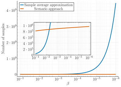
Figure 3: A plot for the number of samples required to achieve a given confidence $1-\beta$ for SAA and the proposed method using the scenario approach. The number of samples reported in this plot is specifically for the vehicle system with 126 regions, as reported in Table I.

VII Conclusions

We studied the problem of certifying probabilistic safety for partially known stochastic systems. The problem is important for the adoption of autonomous safety-critical systems. This safety verification problem was addressed by synthesising Stochastic Barrier Function (SBF)with a data-driven approach leveraging the scenario optimisation theory. To apply the data-driven scenario approach to SBF synthesis, a novel inner chance-constrained approximation to stochastic programming was presented. The chance-constrained approximation was applied to SBFs in Theorem 1: an important consequence of the theorem is that the method can be easily extended to other classes of systems, e.g. polynomial or more general non-linear systems. Experimental studies showed that our method can certify systems with a confidence that is orders of magnitude greater than the state-of-the-art methods, while also producing tighter bounds and being faster.

VIII Technical proofs

VIII-A Proof for Theorem 1

In order to prove Theorem 1 we consider the following stochastic program, which generalizes Problem (BP),

$$\min_{z} \quad s^{\top}z$$ (14)

$$\operatorname{s.t.} \quad\mathbb{E}\left\{g(x,z,\eta(\omega))\right\}\leq h(x,z),\quad\text{ for all }x\in{\mathcal{S}},$$

where $z\in\mathbb{R}^{d}$ is the decision variable, $s\in\mathbb{R}^{d}$ is the cost vector, $\eta:\Omega\to\mathbb{R}^{m}$ is a random variable on $(\Omega,\mathcal{F},\mathbb{P})$, and $g:\mathbb{R}^{n}\times\mathbb{R}^{d}\times\mathbb{R}^{m}\to\mathbb{R}$ is a measurable and integrable function for each pair $(x,z)\in\mathbb{R}^{n}\times\mathbb{R}^{d}$, $h:\mathbb{R}^{n}\times\mathbb{R}^{d}\to\mathbb{R}_{\geq 0}$ is a function, and ${\mathcal{S}}$ is a measureable set on $\mathbb{R}^{n}$. The feasible set of Problem (14) is given by

$$\mathcal{Z}=\{z\in\mathbb{R}^{d}:\mathbb{E}\{g(x,z,\eta(\omega))\}\leq h(x,z)\text{ for all }x\in{\mathcal{S}}\}.$$

Theorem 3 shows that an inner approximation of the feasible set $\mathcal{Z}$ for Problem (14) can be obtained through a chance-constrained problem. Thus, we can relax Problem (14) to the following chance-constrained problem.

Theorem 3 (Inner chance-constrained approximation)

Let $\epsilon\in(0,1)$ be a given threshold and assume $h(x,z)\geq 0$ for all $(x,z)\in\mathbb{R}^{n}\times\mathbb{R}^{d}$. Define a uniform upper bound $M=\sup\limits_{x,z,\omega}g(x,z,\eta(\omega))>0$ on $g$ and let ${\nu}\geq\frac{\epsilon M}{1-\epsilon}$. Define the set

$$E(x,z)=\left\{\omega\in\Omega:g(x,z,\eta(\omega))+{\nu}\leq h(x,z)\right\},$$

and consider the chance-constrained problem

$$\min_{z} \quad s^{\top}z$$ (15)

$$\operatorname{s.t.} \quad\mathbb{P}\left\{E(x,z)\right\}\geq 1-\epsilon,\text{ for all }x\in{\mathcal{S}},$$

whose feasible set is given by $\mathcal{Z}^{\prime}=\big{\{}z\in\mathbb{R}^{d}:\mathbb{P}\left\{E(x,z)\big{\}}\geq 1-\epsilon,\text{ for all }x\in{\mathcal{S}}\right\}$. Then we have that $\mathcal{Z}^{\prime}\subseteq\mathcal{Z}$.

Proof:

Pick any $\bar{z}\in\mathcal{Z}^{\prime}$. Our goal is to show that $\bar{z}\in\mathcal{Z}$. To this end, pick any $x\in{\mathcal{S}}$ and notice that

$$\mathbb{E}\left[g(x,\bar{z},\eta(\omega))\right]= \int_{E(x,\bar{z})}g(x,\bar{z},\eta(\omega))\,d\mathbb{P}(\omega)+$$

$$\int_{E(x,\bar{z})^{c}}g(x,\bar{z},\eta(\omega))\,d\mathbb{P}(\omega).$$

Hence, we can derive the following

$$\mathbb{E}\left\{g(x,\bar{z},\eta(\omega))\right\}$$ (16)

$$\quad\;\leq(h(x,\bar{z})-{\nu})\mathbb{P}\{E(x,\bar{z})\}+M\mathbb{P}\{E(x,\bar{z})^{c}\}$$

$$\quad\;=h(x,\bar{z})-{\nu}\mathbb{P}\{E(x,\bar{z})\}+M\mathbb{P}\{E(x,\bar{z})^{c}\}$$

where the first inequality follows from the fact that $g(x,\bar{z},\eta(\omega))$ is less than or equal to $h(x,\bar{z})-{\nu}$ on the set $E(x,\bar{z})$ and that $g$ is uniformly upper bounded by $M$ on the whole space $\Omega$. and the second inequality follows from $h(x,\bar{z})\geq 0$ for all $(x,\bar{z})\in\mathbb{R}^{n}\times\mathbb{R}^{d}$ and $\mathbb{P}\{E(x,\bar{z})\}\in[0,1]$.

Now, by transitivity it holds that $\mathbb{E}\left\{g(x,\bar{z},\eta(\omega))\right\}\leq h(x,\bar{z})$ if $h(x,\bar{z})-{\nu}\mathbb{P}\{E(x,\bar{z})\}+M\mathbb{P}\{E(x,\bar{z})^{c}\}\leq h(x,\bar{z})$. Due to the feasibility of $\bar{z}$, it holds that $\mathbb{P}\{E(x,\bar{z})\}\geq 1-\epsilon$ and $\mathbb{P}\{E(x,\bar{z})^{c}\}\leq\epsilon$. Furthermore, observe that ${\nu}\geq 0$ and $M>0$, hence the second inequality holds if $-{\nu}\mathbb{P}\{E(x,\bar{z})\}+M\mathbb{P}\{E(x,\bar{z})^{c}\}\leq 0$. Restructuring this inequality, we arrive at ${\nu}\geq\frac{\epsilon M}{1-\epsilon}$, which is assumed to hold (by carefully choosing ${\nu}$). Therefore, we observe that $\bar{z}\in\mathcal{Z}$, thus concluding the proof of the theorem. ∎

What is left to show to conclude the proof is to show that $g(x,z,\eta(\omega))=B(f(x)+\eta(\omega),\theta)$ and $h(x,z)=B(x)+{c}$ satisfies the conditions of Theorem 3, i.e., $h$ is non-negative and $g$ is uniformly bounded by $M$. Non-negative follows trivially by the definition of a SBF, while boundedness of $B$ and consequently of $g$, can always be enforced.

References

- [1] Shai Shalev-Shwartz, Shaked Shammah and Amnon Shashua “On a Formal Model of Safe and Scalable Self-driving Cars” In arXiv preprint arXiv:1708.06374, 2017
- [2] Scott C. Livingston, Richard M. Murray and Joel W. Burdick “Backtracking temporal logic synthesis for uncertain environments” In ICRA, 2012
- [3] Alessandro Abate, Maria Prandini, John Lygeros and Shankar Sastry “Probabilistic reachability and safety for controlled discrete time stochastic hybrid systems” In Automatica, 2008
- [4] Nathalie Cauchi et al. “Efficiency through uncertainty: Scalable formal synthesis for stochastic hybrid systems” In HSCC, 2019, pp. 240–251
- [5] Stephen Prajna, Ali Jadbabaie and George Pappas “A framework for worst-case and stochastic safety verification using barrier certificates” In IEEE TAC, 2007
- [6] Cesar Santoyo, Maxence Dutreix and Samuel Coogan “A barrier function approach to finite-time stochastic system verification and control” In Automatica, 2021
- [7] Ibon Gracia, Dimitris Boskos, Luca Laurenti and Manuel Mazo “Distributionally Robust Strategy Synthesis for Switched Stochastic Systems” In HSCC, 2023
- [8] Hamed Rahimian and Sanjay Mehrotra “Distributionally robust optimization: A review” In arXiv preprint arXiv:1908.05659, 2019
- [9] Alexander Shapiro, Darinka Dentcheva and Andrzej Ruszczski “Lectures on stochastic programming” Society for Industrial & Applied Mathematics, 2021
- [10] Harold J Kushner “Stochastic stability and control”, 1967
- [11] Pushpak Jagtap, Sadegh Soudjani and Majid Zamani “Temporal Logic Verification of Stochastic Systems Using Barrier Certificates” In ATVA, 2018
- [12] Ali Salamati and Majid Zamani “Safety Verification of Stochastic Systems: A Repetitive Scenario Approach” In IEEE Control Systems Letters, 2023
- [13] Alessandro Abate et al. “Quantitative Verification With Neural Networks For Probabilistic Programs and Stochastic Systems” In arXiv preprint arXiv:2301.06136, 2023
- [14] Rayan Mazouz et al. “Safety Guarantees for Neural Network Dynamic Systems via Stochastic Barrier Functions” In NeurIPS, 2022
- [15] Frederik Baymler Mathiesen, Simeon C. Calvert and Luca Laurenti “Safety Certification for Stochastic Systems via Neural Barrier Functions” In IEEE Control Systems Letters, 2023
- [16] Ali Salamati, Abolfazl Lavaei, Sadegh Soudjani and Majid Zamani “Data-Driven Safety Verification of Stochastic Systems via Barrier Certificates” In IFAC-PapersOnLine, 2021
- [17] A. Abate and M. Prandini “Approximate abstractions of stochastic systems: a randomized method” In IEEE CDC, 2011
- [18] Thom S. Badings et al. “Sampling-Based Robust Control of Autonomous Systems with Non-Gaussian Noise” In AAAI Association for the Advancement of Artificial Intelligence (AAAI), 2022
- [19] Thom Badings, Licio Romao, Alessandro Abate and Nils Jansen “Probabilities Are Not Enough: Formal Controller Synthesis for Stochastic Dynamical Models with Epistemic Uncertainty” In AAAI Association for the Advancement of Artificial Intelligence (AAAI), 2023
- [20] Abolfazl Lavaei, Sadegh Soudjani, Emilio Frazzoli and Majid Zamani “Constructing MDP Abstractions Using Data With Formal Guarantees” In IEEE Control Systems Letters, 2023
- [21] John Jackson, Luca Laurenti, Eric Frew and Morteza Lahijanian “Strategy synthesis for partially-known switched stochastic systems” In HSCC, 2021
- [22] Kazumune Hashimoto et al. “Learning-based symbolic abstractions for nonlinear control systems” In Automatica, 2022
- [23] Stephen Boyd and Lieven Vandenberghe “Convex Optimization” Cambride University Press, 2004
- [24] Marco Campi and Simone Garatti “The exact feasibility of randomized solutions of uncertain convex programs” In SIAM Journal on Optimization, 2008
- [25] Pushpak Jagtap, Sadegh Soudjani and Majid Zamani “Formal Synthesis of Stochastic Systems via Control Barrier Certificates” In IEEE TAC, 2020
- [26] Marco C. Campi, Simone Garatti and Maria Prandini “The scenario approach for systems and control design” In Annual Reviews in Control, 2009