Wave reflections and resonance in a Mach 0.9 turbulent jet

Abstract

This work aims to provide a more complete understanding of the resonance mechanisms that occur in turbulent jets at high subsonic Mach number, as shown by Towne et al. (2017). Resonance was suggested by that study to exist between upstream- and downstream-travelling guided waves. Five possible resonance mechanisms were postulated, each involving different families of guided waves that reflect in the nozzle exit plane and a number of downstream turning points. But the study did not show which of these mechanisms are active in the flow. In this work, the waves underpinning resonance are identified via a biorthogonal projection of the Large Eddy Simulation data on eigenbases provided by locally parallel linear stability analysis. Two of the scenarios postulated by Towne et al. (2017) are thus confirmed to exist in the turbulent jet data. The reflection-coefficients in the nozzle exit and turning-point planes are, furthermore, identified.

1 Introduction

The mechanisms underpinning oscillator behaviour in fluid-mechanics problems can be classified as short- or long-ranged. Short-ranged mechanisms are typically associated with absolute instability (Huerre & Monkewitz, 1985), observed for instance in wakes (Monkewitz & Sohn, 1988) and hot jets (Huerre & Monkewitz, 1990). Long-ranged mechanisms involve a pair of upstream- and downstream-travelling waves which interact at two end locations, where they are reflected into one another. If the wave amplitude increases over the cycle between two reflections, a long-range-resonant instability occurs. If the amplitude is unchanged, a neutrally stable mode is created, which, in turbulent flows, can be driven by the background turbulence. Such mechanisms have been observed in many different flows, such as when jets interact with edges (Powell, 1953; Jordan et al., 2018), in cavity flows (Rockwell & Naudascher, 1979; Rowley et al., 2002), impinging jets (Ho & Nosseir, 1981; Tam & Ahuja, 1990), shock-containing jets (Raman, 1999; Edgington-Mitchell, 2019), and high subsonic jets (Towne et al., 2017; Schmidt et al., 2017). The waves underpinning resonance can frequently be modelled using linear mean-flow analysis (Michalke, 1970; Crighton & Gaster, 1976; Jordan & Colonius, 2013; Cavalieri et al., 2019).

In this study, we revisit the tones found in Mach $0.9$ turbulent jets, postulated by Towne et al. (2017) to be driven by waves resonating between the nozzle exit and downstream turning points. The waves in question are guided waves of positive and negative generalised group velocities, denoted as $k^{+}$ and $k^{-}$ respectively, as per Briggs (1964) and Bers (1983). The waves are neutrally stable at the resonance frequencies and can be described using locally parallel linear stability analysis. Among the identified waves are the Kelvin-Helmhotz (hereafter K-H) instability wave (Michalke, 1970) and neutrally stable guided waves (Towne et al., 2017; Martini et al., 2019). These guided waves consist of one downstream-travelling wave: the $k^{+}$ duct-like mode and two upstream-travelling waves: the $k^{-}$ duct-like mode and $k^{-}$ discrete free-stream mode.

At resonant frequencies, the $k^{+}$ and $k^{-}$ waves propagate between the nozzle exit and turning point, exchanging energy through reflections at these end locations. The turning point is a downstream location characterized by the presence of a saddle point where a pair of $k^{+}$ and $k^{-}$ waves share the same frequency and wavenumbers. Depending on the frequency, the $k^{+}$ wave can form a turning point with either of the $k^{-}$ waves, resulting in two possible resonance mechanisms (Towne et al., 2017). The stability analysis (see section 3.1) reveals that, in the Strouhal range ($St=fD/U_{j}=\{0.23$ $-$ $0.47\}$, where $f$ is the resonance frequency, $U_{j}$ is the jet velocity, and $D$ is the jet diameter), the $k^{+}$ duct-like mode forms a turning point with the $k^{-}$ duct-like mode for lower frequencies, but with the $k^{-}$ discrete free-stream mode for higher frequencies.

In the present work, we aim to conclusively establish if these frequency-dependent resonance mechanisms are active in the jet. We revisit the turbulent jet data with the goal of: (1) educing the waves present in the data; (2) establishing which of these underpin resonance; (3) computing the reflection-coefficients associated with energy exchange at the resonance end locations. This third objective is important for simplified resonance models, such as proposed by Jordan et al. (2018); Mancinelli et al. (2019, 2021).

The paper is organised as follows. Section 2 presents the Large Eddy Simulation (LES) database which is used. Local linear stability analysis is performed on the jet mean flow in section 3.1. The LES data is then decomposed using bi-orthogonal projections on the stability eigenbasis in section 3.2. It is shown how, at resonant conditions, the LES data can be represented by a rank-4 model. This is the basis for the calculation of reflection-coefficients at the resonance end locations. Section 4 presents the reflection-coefficient eduction methodology and section 5 presents the final results for a range of resonant frequencies.

2 LES database

We analyze LES data for a Mach $M=0.9$ jet from Brès et al. (2018), where the guided waves have been observed in the potential-core region and associated discrete spectral tones have been detected in the near-nozzle region (Towne et al., 2017; Schmidt et al., 2017; Bogey, 2021).

The data, described in Brès et al. (2018), covers a cylindrical grid with length $30D$ and radius $6D$. It contains $10000$ timesteps over $2000$ acoustic time units ($tc/D$, where $c$ is sound speed), sampled every $0.2$ acoustic time units. The cylindrical coordinate system has its origin centered on the jet axis in the nozzle plane.

LES time-series data is decomposed into Fourier modes,

$$\textbf{q}_{LES}(x,r,\theta,t)=\sum_{\omega}\sum_{m}\mathbf{\hat{q}}_{LES}(x,r,m,\omega)\hskip 3.69885pte^{im\theta}e^{i\omega t},$$ (1)

where $x$ is the axial coordinate, $r$ is the radial coordinate, $m$ is the azimuthal wavenumber and $\omega$ is the angular frequency of fluctuation quantities. The time-series is split into 153 realisations, where each realisation contains 256 snapshots and an overlap of 75$\%$. This leads to the frequency resolution of $\Delta St=\Delta fD/U_{j}=0.0217$. Only the $m=0$ mode is considered.

3 Decomposing turbulent jet data into the resonating modes

To identify the waves that dominate the jet dynamics at the resonant frequencies, the LES data at a given streamwise station is projected onto eigenmodes obtained from a locally parallel linear stability analysis that is described in the following section.

3.1 Local Stability Analysis

Stability analysis is performed around the LES turbulent mean flow. To obtain a smooth flow, the radial profile of the LES mean flow is fitted with the analytical profile

$$\overline{U}_{x}(r)=\frac{U_{j}}{2}\bigg{[}1+tanh\bigg{\{}b\bigg{(}\frac{0.5}{r/D}-\frac{r/D}{0.5}\bigg{)}\bigg{\}}\bigg{]},$$ (2)

where $b$ is the fitting parameter.

Fluctuating quantities are described by the vector $\mathbf{q}^{\prime}=\left[\begin{array}[]{ccccc}\boldsymbol{\rho}^{\prime}&\mathbf{u}_{x}^{\prime}&\mathbf{u}_{r}^{\prime}&\mathbf{u}_{\theta}^{\prime}&\mathbf{T}^{\prime}\end{array}\right]^{\top}$, where $\top$ represents the transpose, $\boldsymbol{\rho}^{\prime}$ the density, $\mathbf{u}_{x}^{\prime}$ the streamwise velocity, $\mathbf{u}_{r}^{\prime}$ the radial velocity, $\mathbf{u}_{\theta}^{\prime}$ the azimuthal velocity and $\mathbf{T}^{\prime}$ the temperature. Normal-mode ansatz,

$$\mathbf{q}^{\prime}=\mathbf{\hat{q}}(r)e^{i\alpha x}e^{im\theta}e^{-i\omega t},$$ (3)

where $\mathbf{\hat{q}}$ gives the radial structure and $\alpha$ is the axial wavenumber, allows the linearised N-S equations to be compactly written as,

$$\mathbf{M}\mathbf{\hat{q}}=i\alpha\mathbf{\hat{q}}.$$ (4)

The eigenmodes are normalised such that each mode has: (1) $0^{o}$ phase angle for the streamwise velocity fluctuation at the jet axis ($\angle\mathbf{\hat{u}}_{x}=0^{o}$ at $r=0$); and (2) unit Energy norm, $E$ (Chu, 1965), defined as

$$\mathrm{E}=\int_{0}^{\infty}\Bigg{[}\frac{\overline{T}}{\gamma\overline{\rho}M_{j}^{2}}\mid\boldsymbol{\hat{\rho}}\mid^{2}+\overline{\rho}\mid\mathbf{\hat{u}}_{x}\mid^{2}+\overline{\rho}\mid\mathbf{\hat{u}}_{r}\mid^{2}+\overline{\rho}\mid\mathbf{\hat{u}}_{\theta}\mid^{2}+\frac{\overline{\rho}}{\gamma(\gamma-1)\overline{T}M_{j}^{2}}\mid\mathbf{\hat{T}}\mid^{2}\Bigg{]}r\hskip 2.84526ptdr.$$ (5)

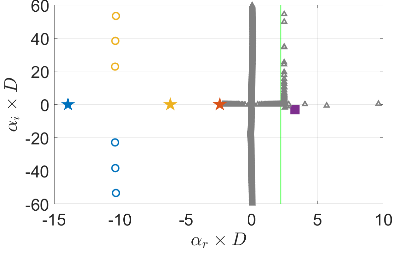
(a) Eigenspectrum for $St=0.39$: $({\star}$, blue) $k^{-}_{d}$; $({\star}$, red) $k^{-}_{p}$; $({\star}$, yellow) $k^{+}_{T}$; $({\blacksquare}$, purple) $k^{+}_{KH}$; ( , light green) sonic line.

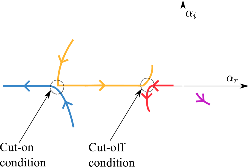
(b) Modes trajectories for $St$={$0.23$ $\rightarrow$ $0.47$}: ( , blue) $k^{-}_{d}$; ( , red) $k^{-}_{p}$; ( , yellow) $k^{+}_{T}$; ( , purple) $k^{+}_{KH}$.

Figure 1: Linear stability analysis at $x/D=0$, $m=0$ for $M=0.9$ jet.

Stability analysis is performed for $m=0$ and over the frequency range, $0.23\leq St\leq 0.47$. The eigenspectrum for one of the tonal frequencies, $St=0.39$, is shown in figure 1(a).

Various families of modes can be seen in figure 1(a), where real and imaginary parts of $\alpha$ are represented on the horizontal and vertical axes respectively. The $k^{+}_{KH}$ (K-H mode marked with a square) is the only unstable mode of the system which leads to amplitude growth of the coherent part of the fluctuation field which then stabilises and decays, forming a wavepacket (Jordan & Colonius, 2013).

The resonating modes leading to tones are marked with stars and are named as per Jordan et al. (2018). They are guided propagative modes resonating between the end locations and are the focus of the present work. The resonance loop consists of a downstream travelling mode ($k^{+}_{T}$) and an upstream travelling mode ($k^{-}_{d}$ and/or $k^{-}_{p}$). Modes $k^{+}_{T}$ and $k^{-}_{d}$ correspond to the acoustic waves trapped within the potential core and they belong to the families of the infinite number of such modes (marked by circles). Further details about these modes can be found in Towne et al. (2017), Schmidt et al. (2017) and Martini et al. (2019).

In figure 1(a), the modes in the first quadrant with subsonic phase speed (the sonic line is at $\alpha_{r}=\omega/c$) are stable and are distributed in two separate branches.: a near-horizontal branch consisting of critical layer modes that have support in the shear layer, and a near-vertical branch with eigenfunctions that have support in the core region of the jet (Rodríguez et al., 2015).

Although all guided modes are propagative at $St=0.39$, this is not the case for all $St$. Figure 1(b) shows the trajectories of the four modes in the complex $\alpha$ plane as $St$ varies from $0.23$ to $0.47$. At $St=0.23$, $k^{+}_{T}$ and $k^{-}_{d}$ are evanescent, and they move gradually towards the $\alpha_{i}=0$ axis and overlap at saddle-point 1, defining a cut-on condition at $St=0.37$ (Towne et al., 2017). The modes remain propagative until saddle-point 2, a cut-off condition, which occurs at $0.428$, where $k^{+}_{T}$ and $k^{-}_{p}$ modes meet. For $St>0.428$, the $k^{+}_{T}$ and $k^{-}_{p}$ modes become evanescent. At higher frequencies, other modes from the families of $k^{+}_{T}$ and $k^{-}_{d}$ cut on leading to resonance, but these scenarios are not considered in the present work since the most energetic resonance occurs for the considered scenario.

3.2 Educing mode amplitudes by bi-othogonal projections

We here aim to educe amplitudes of the K-H mode, which is the main instability of the jet, and the three guided waves, which are postulated to be responsible for the observed tones. Due to the non-orthogonality of the system, mode amplitudes are obtained by bi-orthogonal projection as per Rodríguez et al. (2013, 2015).

A basis for bi-orthogonal projection is constructed from the adjoint system,

$$\mathbf{M}^{H}\mathbf{\hat{q}}^{+}=i\alpha^{+}\mathbf{\hat{q}}^{+},$$ (6)

where $H$ represents the Hermitian transpose, $\alpha^{+}$ are the complex conjugate of eigenvalues of the direct system and $\mathbf{\hat{q}}^{+}$ are the adjoint eigenfunctions that we seek.

The adjoint eigenfunctions are normalized such that,

$$(\mathbf{\hat{q}}^{+}_{i})^{H}\mathbf{\hat{q}}_{i}=1,$$ (7)

where $i$ is the index of the mode being normalized.

Before projection, $\mathbf{\hat{q}}_{LES}$ (from (1)) is interpolated onto the Chebyshev nodes, on which the eigenfunctions are defined, using Piecewise Cubic Hermite Interpolating Polynomials. Due to the fast decay of disturbances away from the jet, the points outside the available LES grid locations are assigned a value of $0$ for the fluctuation quantities. This is corroborated by verifying that $\mid(\mathbf{\hat{q}}^{+}_{i})^{H}\hskip 2.84526pt\mathbf{\hat{q}}_{i}\mid$ is almost the same with or without this assumption $\forall St,\forall i$, and hence the projection amplitudes would be negligibly affected.

The mode amplitudes are then obtained by biorthogonal projection,

$$a_{i}^{n}={(\mathbf{\hat{q}}^{+}_{i})^{H}\hskip 0.28453pt\hskip 2.84526pt\mathbf{\hat{q}}_{LES}^{n}},$$ (8)

where $\mathbf{\hat{q}}_{LES}^{n}$ is the LES fluctuation data from the $n^{th}$ realisation; and $a_{i}^{n}$ is the expansion coefficient that defines the contribution of the $i^{th}$ mode to the flow state in the $n^{th}$ realisation, giving the amplitude and the phase of mode.

In figure 2(a), radial profiles of the streamwise velocity for a selection of modes at the nozzle exit plane and for St = 0.39 are compared with the power spectral density (PSD) computed from the LES data. The guided modes have substantial magnitudes, consistent with the resonance phenomenon observed at this tonal frequency. It is also clear that within the jet core, the $k^{-}_{d}$ and $k^{+}_{T}$ dominate the fluctuation field. In the shear region, $k^{-}_{d}$, $k^{-}_{p}$ and $k^{+}_{T}$ have comparable levels. On the low-speed side of the shear layer, fluctuations are dominated by $k^{-}_{p}$ and $k^{+}_{T}$. At the nozzle exit plane, negligible KH mode magnitude suggests a rank-3 system locally, but as the KH mode grows exponentially while travelling downstream, the system should be considered rank-4 globally.

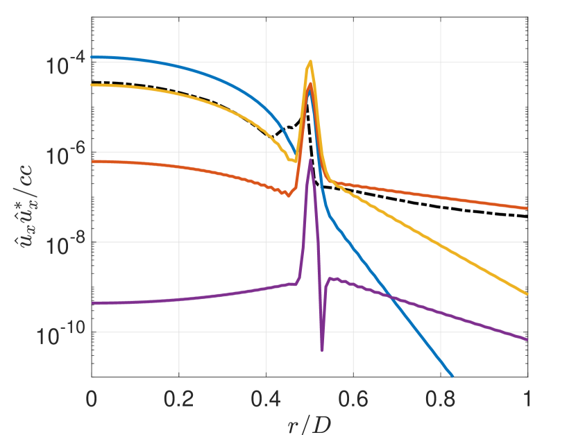
(a) Calibrated $\mathbf{\hat{u}}_{x}$

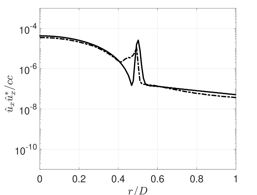
(b) Reconstructed $\mathbf{\hat{u}}_{x}$

Figure 2: Projections for $St=0.39$, $m=0$ at $x/D=0$: ( , dashed black) LES; ( , blue) $k^{-}_{d}$; ( , red) $k^{-}_{p}$; ( , yellow) $k^{+}_{T}$; ( , purple) $k^{+}_{KH}$; ( , black) reconstruction from 4 modes.

A rank-4 reconstruction of the LES data, using these modes, is shown in figure 2(b) along with the LES fluctuation profile. At this resonance frequency, the rank-4 model provides a good overall description of the flow dynamics. We see that in the jet core, the reconstruction amplitude is lesser than the amplitude for the most dominant mode (see $k^{-}_{d}$ in figure 2(a)). This is due to the destructive interference between the modes $k^{-}_{d}$ and $k^{+}_{T}$ as we found them to be antiphase to each other. The mismatch for reconstruction in the mixing layer is likely due to disturbances originating in the nozzle boundary layer, leading to energetic but stable mixing layer modes (Towne & Colonius, 2015).

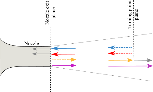
Figure 3: Sketch of waves interacting at the resonance end locations. At the nozzle exit plane: ($\longleftarrow$, blue) incident $k^{-}_{d}$ wave; ($\longleftarrow$, red) incident $k^{-}_{p}$ wave; ($\longleftarrow$, grey) transmitted waves; ($\longrightarrow$, dashed yellow) reflected $k^{+}_{T}$ wave; ($\longrightarrow$, purple) $k^{+}_{KH}$ wave. At the turning point plane: ($\longrightarrow$, yellow) incident $k^{+}_{T}$ wave; ($\longrightarrow$, grey) transmitted wave; ($\longleftarrow$, dashed blue) reflected $k^{-}_{d}$ wave; ($\longleftarrow$, dashed red) reflected $k^{-}_{p}$ wave.

4 Reflection-coefficient eduction

We now present a method used to compute reflection-coefficients between pairs of $k^{-}$ and $k^{+}$ waves at the resonance end locations. Figure 3 shows a schematic of reflections at the nozzle exit plane and the turning point plane. At the turning point, the incident propagative $k^{+}_{T}$ wave can be reflected as a propagative wave ($k^{-}_{d}$ or $k^{-}_{p}$) and transmitted as an evanescent wave. The reflected wave then propagates until it reaches the nozzle exit plane where it is reflected as a $k^{+}_{T}$ wave that travels downstream until the turning point, hence completing the resonance loop. The relation of magnitude and phases of these waves among each other are described by reflection and transmission coefficients at the corresponding end locations. Note that at the nozzle plane, apart from the contribution from $k^{-}_{d}$ or $k^{-}_{p}$ waves, $k^{+}_{T}$ wave may also be driven by nozzle fluctuations, or by the reflection of other $k^{-}$ waves.

4.1 Coherence analysis

Before evaluating the reflection-coefficients, we examine the relation between expansion coefficient signals from the modes through the coherence function,

$$\gamma^{2}_{ij}=\frac{\langle{a}_{i}{a}_{j}^{H}\rangle^{2}}{\langle{a}_{i}{a}_{i}^{H}\rangle\hskip 2.84526pt\langle{a}_{j}{a}_{j}^{H}\rangle},$$ (9)

(a) Coherence function

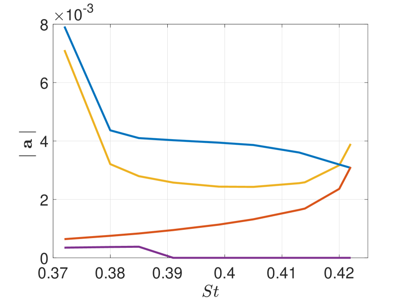
(b) Mode amplitudes

Figure 4: At the nozzle exit, $x/D=0$. (a) Coherence function: ( , blue) $k_{d}^{-}/k_{T}^{+}$; ( , red) $k_{p}^{-}/k_{T}^{+}$; ( , yellow) $k_{d}^{-}/k_{p}^{-}$; ( , purple) $k_{d}^{-}/k_{KH}^{+}$; ( , dashed purple) $k_{p}^{-}/k_{KH}^{+}$. (b) Mode amplitudes: ( , blue) $k^{-}_{d}$; ( , red) $k^{-}_{p}$; ( , yellow) $k^{+}_{T}$; ( , purple) $k^{+}_{KH}$.

where ${a}_{i}$ and ${a}_{j}$ are the expansion coefficients (see (8)) for the two modes, and $\langle\cdot\rangle$ represents the expected value, which is an estimate from the available samples.

For the present system of modes, coherence-function dependence on $St$ at $x/D=0$ can be seen in figure 4(a). For low $St$, a strong coherence is observed between $k^{-}_{d}$ and $k_{T}^{+}$ which signifies that the $k^{-}_{d}/k_{T}^{+}$ resonance pair is active at these frequencies.

As $St$ increases, the coherence function decays for $k^{-}_{d}/k^{+}_{T}$ while rising sharply for $k^{-}_{p}/k^{+}_{T}$. This suggests a change in the resonance mechanism, as frequency increases, towards a scenario where the $k^{-}_{p}/k^{+}_{T}$ pair is dominant. The small coherence of the $k^{+}_{KH}$ mode ($\gamma^{2}<0.3$) with the $k^{-}$ waves signifies its absence in the resonance mechanisms, and for this reason, it is excluded from the forthcoming discussion.

The variation of mode amplitudes with $St$ at $x/D=0$, as shown in figure 4(b), tells a similar story. At low $St$, the $k_{T}^{+}$ amplitude decays with increasing $St$ following the trend of $k_{d}^{-}$; but at high $St$, it grows with increasing $St$, following the trend of $k_{p}^{-}$, again reflecting a change of the dominant resonant mechanisms with increasing frequency.

4.2 Reflection equations for nozzle exit plane

At the nozzle exit plane, the expansion coefficients of the $k^{+}_{T}$ wave are related to expansion coefficients of $k^{-}$ waves through complex reflection-coefficients as

$${a}_{T}^{+}=R^{d-}\hskip 2.84526pt{a}_{d}^{-}+R^{p-}\hskip 2.84526pt{a}_{p}^{-}+{a}_{o}.$$ (10)

Here, $R^{d-}\hskip 2.84526pt{a}_{d}^{-}$ is the contribution to ${a}_{T}^{+}$ that arises from reflection of ${a}_{d}^{-}$; $R^{p-}\hskip 2.84526pt{a}_{p}^{-}$ is the contribution from reflection of ${a}_{p}^{-}$; ${a}_{o}$ groups all other contributions, e.g., reflections of other waves or disturbances coming from within the nozzle.

To evaluate the reflection-coefficients $R^{d-}$ and $R^{p-}$, following the procedure of Bendat & Piersol (2011), we multiply (10) with both ${{a}_{d}^{-}}^{H}$ and ${{a}_{p}^{-}}^{H}$ and take the expected value, giving

$$\langle{a}_{T}^{+}{{a}_{d}^{-}}^{H}\rangle=R^{d-}\langle{a}_{d}^{-}{{a}_{d}^{-}}^{H}\rangle+R^{p-}\langle{a}_{p}^{-}{{a}_{d}^{-}}^{H}\rangle+\langle{a}_{o}{{a}_{d}^{-}}^{H}\rangle,$$ (11)

$$\langle{a}_{T}^{+}{{a}_{p}^{-}}^{H}\rangle=R^{d-}\langle{a}_{d}^{-}{{a}_{p}^{-}}^{H}\rangle+R^{p-}\langle{a}_{p}^{-}{{a}_{p}^{-}}^{H}\rangle+\langle{a}_{o}{{a}_{p}^{-}}^{H}\rangle.$$ (12)

Contributions from the nozzle boundary layer disturbances and other wave reflections are uncorrelated with the resonance dynamics, and thus we may assume $\langle{a}_{o}{{a}_{d}^{-}}^{H}\rangle=\langle{a}_{o}{{a}_{p}^{-}}^{H}\rangle=0$. With this assumption, (11) and (12) can be solved, expressing the reflection-coefficients, $R^{d-}$ and $R^{p-}$, in terms of expansion coefficient correlations.

4.3 Reflection equations for turning point plane

We now present the system of equations used to calculate the reflection-coefficients at the turning point location where the $k^{+}_{T}$ reflects as $k^{-}_{d}$ and $k^{-}_{p}$ (figure 3). Following a similar procedure to that of section 4.2, we can say that, at the turning point,

$${a}_{d}^{-}=R_{d-}\hskip 2.84526pt{a}_{T}^{+}+{a}_{o}\hskip 28.45274pt\&\hskip 28.45274pt{a}_{p}^{-}=R_{p-}\hskip 2.84526pt{a}_{T}^{+}+{a}_{o},\\$$ (13)

where $R_{d-}$ and $R_{p-}$ are the turning point reflection-coefficients.

Multiplying (13) with ${{a}_{T}^{+}}^{H}$ and taking the expected value gives,

$${\langle{a}_{d}^{-}{{a}_{T}^{+}}^{H}\rangle}=R_{d-}{\langle{a}_{T}^{+}{{a}_{T}^{+}}^{H}\rangle}+\langle{a}_{o}{{a}_{T}^{+}}^{H}\rangle\hskip 8.5359pt\&\hskip 8.5359pt{\langle{a}_{p}^{-}{{a}_{T}^{+}}^{H}\rangle}=R_{p-}{\langle{a}_{T}^{+}{{a}_{T}^{+}}^{H}\rangle}+\langle{a}_{o}{{a}_{T}^{+}}^{H}\rangle.$$ (14)

With the assumption of $\langle{a}_{o}{{a}_{T}^{+}}^{H}\rangle=0$, (14) can be solved for $R_{d-}$ and $R_{p-}$.

5 Results and discussions

5.1 Reflection-coefficients at the resonance end locations

In the nozzle exit plane, the magnitudes and phases of the reflection-coefficients, $R^{d-}$ and $R^{p-}$, are presented as a function of $St$ in figures 5(a) and 5(b). High magnitudes for both the reflection-coefficients indicate strong reflections. We also observe that as $St$ increases, $\mid R^{d-}\mid$ decreases while $\mid R^{p-}\mid$ decreases and then increases. The phase angles for both reflection-coefficients are close to $180^{o}$ indicating out-of-phase reflection.

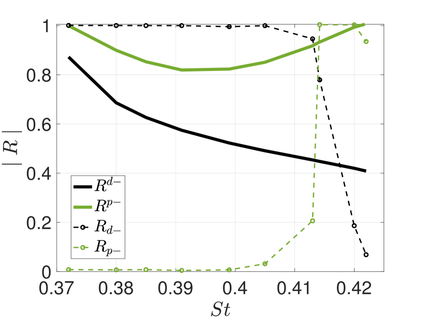
(a) Reflection-coefficient magnitude

(b) Reflection-coefficient phase

Figure 5: Reflection-coefficients. At the nozzle exit: $R^{d-}$ and $R^{p-}$ correspond to the reflection of $k_{d}^{-}$ wave and $k_{p}^{-}$ wave respectively into the $k_{T}^{+}$ wave. At the turning point: $R_{d-}$ and $R_{p-}$ correspond to the reflection of $k_{T}^{+}$ wave into the $k_{d}^{-}$ wave and $k_{p}^{-}$ wave respectively.

At the turning point, the magnitudes and phases of the reflection-coefficients are shown in figures 5(a) and 5(b) as well. From the local stability analysis, the $k_{T}^{+}$ mode is evanescent downstream of the turning point (see figure 1(b)). This implies perfect reflection in the turning-point plane, as beyond here, the $k_{T}^{+}$ mode cannot propagate energy downstream. This is exactly what is found for the reflection-coefficients in the turning-point plane i.e. $\mid R_{d-}\mid\sim 1$ & $\angle R_{d-}\sim 180^{o}$ for the lower $St$ ($0.37<St<0.41$); and $\mid R_{p-}\mid\sim 1$ & $90<\angle R_{p-}<180^{o}$ for the higher $St$ ($0.41<St<0.43$).

5.2 Resonance-mechanism dependence on $St$

The results from sections 4 and 5.1 conclude that for the frequency range $0.37<St<0.41$, it is the $k_{d}^{-}/k_{T}^{+}$ pair of modes that resonate while for $0.41<St<0.43$, it is the $k_{p}^{-}/k_{T}^{+}$ pair that resonate. The resonance mechanism switches near $St=0.415$.

These two resonance mechanisms were proposed by Towne et al. (2017). For the lower frequencies, $St=0.39$ for instance, the saddle point at the turning point exists between $k^{-}_{d}$ and $k^{+}_{T}$ modes, which means that the acoustic resonance at $St=0.39$ is being led by the $k^{+}_{T}/k^{-}_{d}$ pair. This is exactly what we see in figures 4 and 5(a), where the $k^{-}_{d}/k^{+}_{T}$ pair of modes has strong coherence and large reflection-coefficient magnitudes.

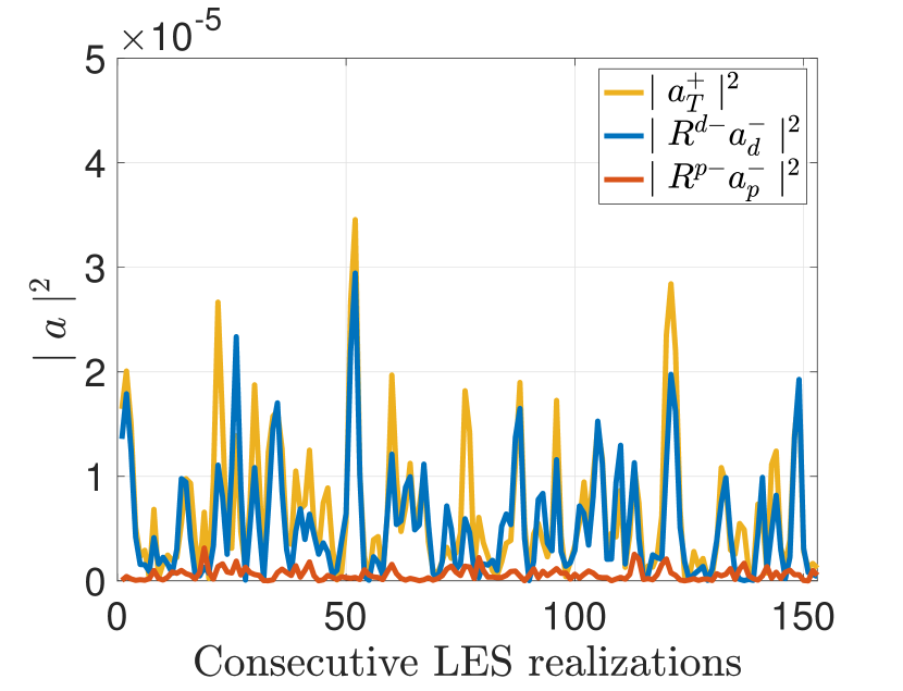
(a) For $St=0.39$

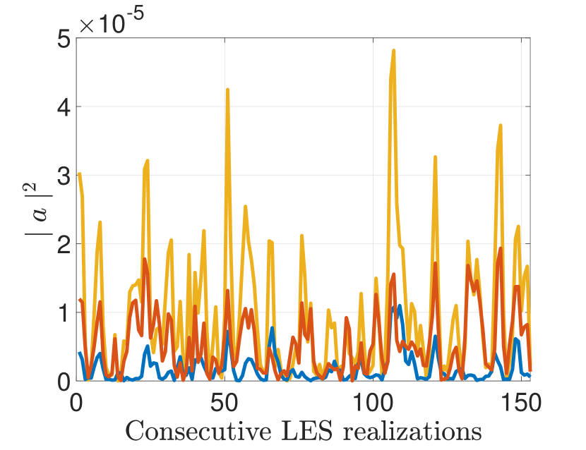
(b) For $St=0.42$

Figure 6: Contribution of $k^{-}_{d}$ and $k^{-}_{p}$ to $k^{+}_{T}$ at $x/D=0$.

For the reflections at the nozzle-exit plane at $St=0.39$, the individual contributions of $k^{-}_{d}$ and $k^{-}_{p}$ to $k^{+}_{T}$ are better seen in figure 6(a) (see (10) for reference). The plot displays the square magnitude of mode amplitudes for $k^{+}_{T}$ (in yellow), as well as the contributions of $k^{-}_{d}$ and $k^{-}_{p}$ (in blue and red, respectively) across consecutive LES realizations. Figure 6(a) demonstrates that $k^{+}_{T}$ is primarily underpinned by reflection of $k^{-}_{d}$. Despite the high magnitude of $R^{p-}$ at the nozzle-exit plane (figure 5(a)), the contribution of the $k^{-}_{p}$ is much smaller than that of $k^{-}_{d}$, due its smaller amplitude (figure 4(b)).

For the higher frequencies, $St=0.42$ for instance, the saddle point at the turning point exists between $k^{-}_{p}$ and $k^{+}_{T}$ modes, hence the acoustic resonance is governed by the $k^{+}_{T}/k^{-}_{p}$ pair. This is also what we observe in figures 4 and 5(a). The individual contributions of $k^{-}_{d}$ and $k^{-}_{p}$ to $k^{+}_{T}$ in the figure 6(b) shows that $k^{+}_{T}$ follows $k^{-}_{p}$ much more closely than $k^{-}_{d}$ at this $St$. Hence, $k^{+}_{T}$ is the direct reflection result of $k^{-}_{p}$ at $St=0.42$.

6 Conclusion

Resonating guided waves in the potential core of a $M=0.9$ turbulent jet which lead to tones previously observed in experiments and numerical simulations (Towne et al., 2017; Brès et al., 2018) have been studied. The resonating guided waves consisted of a downstream-travelling duct-like wave ($k_{T}^{+}$), an upstream-travelling duct-like wave ($k_{d}^{-}$), and an upstream-travelling discrete free-stream wave ($k_{d}^{-}$).

Bi-orthogonal projection of LES data onto eigenmodes obtained from a linear stability analysis based on the turbulent was used to provide amplitudes of the resonating waves at the resonance end locations: the nozzle exit plane and downstream turning points. The dynamics of the flow at resonance frequencies are well described by a rank-4 model, comprising these neutrally stable guided waves and K-H instability waves. The reflection-coefficients at the resonance end locations were computed under the assumption that contributions from non-resonant modes are uncorrelated with the resonant modes. For the range of tonal frequencies, $0.37<St<0.43$, the mode amplitudes, coherence among them, and reflection-coefficients were presented.

Depending on the frequency, either of the $k^{-}$ waves was found to be taking part in the resonance loop i.e. for $0.37<St<0.41$ (F1), the pair $k_{d}^{-}/k_{T}^{+}$ was active while for $0.41<St<0.43$ (F2), the pair $k_{p}^{-}/k_{T}^{+}$ was active. This frequency-dependence of resonance mechanism had exactly been postulated by Towne et al. (2017) where it was shown that the $k_{T}^{+}$ mode forms a turning point, the saddle point where upstream- and downstream-travelling waves exchange energy, with $k_{d}^{-}$ mode in the F1 frequency range and with $k_{p}^{-}$ mode in the F2 frequency range.

References

- Bendat & Piersol (2011) Bendat, J. S. & Piersol, A. G. 2011 Random data: analysis and measurement procedures, , vol. 729. John Wiley & Sons.
- Bers (1983) Bers, A. 1983 Space-time evolution of plasma instabilities-absolute and convective. In Basic plasma physics. 1.
- Bogey (2021) Bogey, Christophe 2021 Acoustic tones in the near-nozzle region of jets: characteristics and variations between mach numbers 0.5 and 2. Journal of Fluid Mechanics 921.
- Brès et al. (2018) Brès, G. A., Jordan, P., Jaunet, V., Le Rallic, M., Cavalieri, A. V. G., Towne, A., Lele, S. K., Colonius, T. & Schmidt, O. T. 2018 Importance of the nozzle-exit boundary-layer state in subsonic turbulent jets. Journal of Fluid Mechanics 851, 83–124.
- Briggs (1964) Briggs, R. J. 1964 Electron-stream interaction with plasmas .
- Cavalieri et al. (2019) Cavalieri, A. V. G., Jordan, P. & Lesshafft, L. 2019 Wave-packet models for jet dynamics and sound radiation. Applied Mechanics Reviews 71 (2).
- Chu (1965) Chu, Boa-Teh 1965 On the energy transfer to small disturbances in fluid flow (part i). Acta Mechanica 1 (3), 215–234.
- Crighton & Gaster (1976) Crighton, D. G. & Gaster, M. 1976 Stability of slowly diverging jet flow. Journal of Fluid Mechanics 77 (2), 397–413.
- Edgington-Mitchell (2019) Edgington-Mitchell, Daniel 2019 Aeroacoustic resonance and self-excitation in screeching and impinging supersonic jets–a review. International Journal of Aeroacoustics 18 (2-3), 118–188.
- Ho & Nosseir (1981) Ho, Chih-Ming & Nosseir, Nagy S 1981 Dynamics of an impinging jet. part 1. the feedback phenomenon. Journal of Fluid Mechanics 105, 119–142.
- Huerre & Monkewitz (1985) Huerre, Patrick & Monkewitz, Peter A. 1985 Absolute and convective instabilities in free shear layers. Journal of Fluid Mechanics 159 (-1), 151, citation Key Alias: huerre1985absolute.
- Huerre & Monkewitz (1990) Huerre, Patrick & Monkewitz, Peter A. 1990 Local and global instabilities in spatially developing flows. Annual review of fluid mechanics 22 (1), 473–537.
- Jordan & Colonius (2013) Jordan, P. & Colonius, T. 2013 Wave packets and turbulent jet noise. Annual review of fluid mechanics 45, 173–195.
- Jordan et al. (2018) Jordan, P., Jaunet, V., Towne, A., Cavalieri, A. V. G., Colonius, T., Schmidt, O. & Agarwal, A. 2018 Jet–flap interaction tones. Journal of Fluid Mechanics 853, 333–358.
- Mancinelli et al. (2019) Mancinelli, M., Jaunet, V., Jordan, P. & Towne, A. 2019 Screech-tone prediction using upstream-travelling jet modes. Experiments in Fluids 60 (1), 22.
- Mancinelli et al. (2021) Mancinelli, Matteo, Jaunet, Vincent, Jordan, Peter & Towne, Aaron 2021 A complex-valued resonance model for axisymmetric screech tones in supersonic jets. Journal of Fluid Mechanics 928.
- Martini et al. (2019) Martini, Eduardo, Cavalieri, André V. G. & Jordan, Peter 2019 Acoustic modes in jet and wake stability. Journal of Fluid Mechanics 867, 804–834.
- Michalke (1970) Michalke, A. 1970 A note on the spatial jet-instability of the compressible cylindrical vortex sheet .
- Monkewitz & Sohn (1988) Monkewitz, Peter A. & Sohn, Kihod 1988 Absolute instability in hot jets. AIAA Journal 26 (8), 911–916.
- Powell (1953) Powell, Alan 1953 On edge tones and associated phenomena. Acta Acustica United with Acustica 3 (4), 233–243.
- Raman (1999) Raman, Ganesh 1999 Supersonic jet screech: half-century from powell to the present. Journal of Sound and Vibration 225 (3), 543–571.
- Rockwell & Naudascher (1979) Rockwell, D & Naudascher, E 1979 Self-sustained oscillations of impinging free shear layers. Annual Review of Fluid Mechanics 11 (1), 67–94.
- Rodríguez et al. (2015) Rodríguez, D., Cavalieri, A. V. G., Colonius, T. & Jordan, P. 2015 A study of linear wavepacket models for subsonic turbulent jets using local eigenmode decomposition of piv data. European Journal of Mechanics-B/Fluids 49, 308–321.
- Rodríguez et al. (2013) Rodríguez, D., Sinha, A., Brès, G. A. & Colonius, T. 2013 Inlet conditions for wave packet models in turbulent jets based on eigenmode decomposition of large eddy simulation data. Physics of Fluids 25 (10), 105107.
- Rowley et al. (2002) Rowley, Clarence W, Colonius, Tim & Basu, Amit J 2002 On self-sustained oscillations in two-dimensional compressible flow over rectangular cavities. Journal of Fluid Mechanics 455, 315–346.
- Schmidt et al. (2017) Schmidt, O. T., Towne, A., Colonius, T., Cavalieri, A. V. G., Jordan, P. & Brès, G. A. 2017 Wavepackets and trapped acoustic modes in a turbulent jet: coherent structure eduction and global stability. Journal of Fluid Mechanics 825, 1153–1181.
- Tam & Ahuja (1990) Tam, Christopher KW & Ahuja, KK 1990 Theoretical model of discrete tone generation by impinging jets. Journal of Fluid Mechanics 214, 67–87.
- Towne et al. (2017) Towne, A., Cavalieri, A. V. G., Jordan, P., Colonius, T., Schmidt, O., Jaunet, V. & Brès, G. A. 2017 Acoustic resonance in the potential core of subsonic jets. Journal of Fluid Mechanics 825, 1113–1152.
- Towne & Colonius (2015) Towne, Aaron & Colonius, Tim 2015 One-way spatial integration of hyperbolic equations. Journal of Computational Physics 300, 844–861.