Temperatures of AdS₂ black holes and holography revisited

Abstract

In a dilaton gravity model, we revisit the calculation of the temperature of an evaporating black hole that is initially formed by a shock wave, taking into account the quantum backreaction. Based on the holographic principle, along with the assumption of a boundary equation of motion, we show that the black hole energy is maintained for a while during the early stage of evaporation. Gradually, it decreases as time goes on and eventually vanishes. Thus, the Stefan-Boltzmann law tells us that the black hole temperature, defined by the emission rate of the black hole energy, starts from zero temperature and reaches a maximum value at a critical time, and finally vanishes. It is also shown that the maximum temperature of the evaporating black hole never exceeds the Hawking temperature of the eternal AdS₂ black hole. We discuss physical implications of the initial zero temperature of the evaporating black hole.

I Introduction

sec:introduction Many years ago, Jackiw Jackiw:1984je and Teitelboim Teitelboim:1983ux proposed a dilaton gravity model for two-dimensional anti-de Sitter (AdS₂) space. It is known that any excitation with finite energy causes significant backreaction on the AdS spacetime Maldacena:1998uz ; Strominger:1998yg . Almheiri and Polchinski (AP) Almheiri:2014cka further developed a modified model that provides a regulated quantum backreaction, which allows one to set up a more meaningful holographic dictionary through the analysis of the black hole in the Hartle-Hawking state Hartle:1976tp ; Israel:1976ur . From the fact that the time coordinate becomes dynamical on the boundary Maldacena:2016upp , the black hole in the Unruh state Unruh:1976db was investigated by assuming a dynamical boundary equation of motion in the AP model Engelsoy:2016xyb . In fact, in a wide variety of cases of two-dimensional toy models, there has been much attention to the backreaction issue that exhibits black hole formation and evaporation Callan:1992rs ; Giddings:1992ff ; Russo:1992ax ; Keski-Vakkuri:1993ybv ; Liberati:1994za ; Navarro-Salas:1995lmi ; Fabbri:1995bz ; Bose:1995bk ; Nojiri:1997sr ; Kim:1998wy ; Spradlin:1999bn ; Fabbri:2005mw ; Almheiri:2019psf .

In particular, the black hole temperature characterizing Hawking radiation plays an important role in black hole thermodynamics, along with the black hole entropy. The common wisdom is that black holes in thermal equilibrium have a constant temperature that can be calculated from the surface gravity method on the black hole side or from the Stefan-Boltzmann law for radiation in a bath side. On the other hand, in evaporating black holes, the calculation of the black hole temperature would be non-trivial since the quasi-static temperature is also assumed to be time-dependent, and thus sensitive to the backreaction of geometry. A recent study in the AP model Engelsoy:2016xyb shows that the initial temperature of the black hole starts from the Hawking temperature and finally vanishes when taking into account the quantum backreaction. In the end, the black hole temperature approaches zero, which implies that the radiation temperature should also be zero in the quasi-equilibrium assumption. Now, one might wonder how the black hole temperature could suddenly become the Hawking temperature as soon as the black hole forms from collapsing matter. It might take some time for the black hole to be thermalized and become a thermal object Hayden:2007cs .

In this work, we use the holography principle Almheiri:2014cka in order to revisit the calculations of the temperature of the evaporating AdS₂ black hole in the AP model. We adopt the dynamical equation of motion proposed in Ref. Engelsoy:2016xyb and properly take into account the effect of quantum backreaction. Consequently, we show that the black hole temperature is initially zero and reaches a maximum temperature less than the Hawking temperature, before finally approaching zero temperature.

The organization of the paper is as follows: In Sec. LABEL:sec:Preliminaries, we employ holographic renormalization process to derive the holographic stress tensor in the AP model and present the general form of the black hole energy associated with various vacuum conditions. In Sec. LABEL:sec:The_Black_hole_in_Equilibrium, we compute the energy and temperature of the eternal AdS₂ black hole by utilizing the energy expression presented in Sec. LABEL:sec:Preliminaries. Our calculations confirm the well-established outcomes in the Hartle-Hawking vacuum state. In Sec. LABEL:sec:The_Black_hole_in_Evaporation, we study the black hole energy in the evaporating AdS₂ black hole and find a different type of temperature in the Unruh vacuum state. Finally, we give our conclusions and discuss our results in Sec. LABEL:sec:conclusion.

II The Holographic stress tensor

sec:Preliminaries In this section, we introduce the two-dimensional dilaton gravity model, which is described by the action consisting of the AP action with classical and quantum matter Almheiri:2014cka :

$$S =S_{\rm AP}+S_{\rm matt}=S_{\rm AP}+S_{\rm cl}+S_{\rm qt},\label{eq:totalaction}$$ (1)

$$S_{\rm AP} =\frac{1}{16\pi G}\int\differential[2]{x}\sqrt{-g}\left[\Phi^{2}(R+2)-2\right]+\frac{1}{8\pi G}\int\differential x^{0}\sqrt{-\gamma}\Phi^{2}K,\label{eq:APaction}$$ (2)

$$S_{\rm cl} =-\frac{1}{2}\int\differential[2]{x}\sqrt{-g}\sum_{i=1}^{N}(\nabla f_{i})^{2},\label{eq:classicalmatteraction}$$ (3)

$$S_{\rm qt} =-\frac{N}{24\pi}\int\differential[2]{x}\sqrt{-g}\left[(\nabla\chi)^{2}+\chi R\right]-\frac{N}{12\pi}\int\differential x^{0}\sqrt{-\gamma}\chi K.\label{eq:quantummatteraction}$$ (4)

Here, $\Phi^{2}$, $f_{i}$, and $K$ represent the dilaton field, scalar matter fields, and the extrinsic curvature, respectively. The auxiliary scalar field $\chi$ is used to localize the non-local Polyakov action Polyakov:1981rd . (For a review, see Vassilevich:2003xt .) The matter contribution is usually subdominant compared to the gravitational contribution. This observation is based on the matter CFT calculation Yang:2018gdb ; Mertens:2022irh . The one-loop Polyakov action for matter fields will be considered within the large $N$ approximation with $\Phi^{-2}N$ being fixed so that the matter part becomes comparable to the gravitational part Strominger:1994tn .

In the conformal gauge of $\differential s^{2}=-e^{2\omega(u,v)}\differential u\differential v$, where $u=t+\sigma$ and $v=t-\sigma$, the equations of motion are given as follows:

$$4\partial_{u}\partial_{v}\omega+e^{2\omega} =0,\label{eq:metriceq}$$ (5)

$$2\partial_{u}\partial_{v}\Phi^{2}+(\Phi^{2}-1)e^{2\omega} =16\pi GT_{uv},\label{eq:dilatonuv}$$ (6)

$$-e^{2\omega}\partial_{u}(e^{-2\omega}\partial_{u}\Phi^{2}) =8\pi GT_{uu},\label{eq:dilatonuu}$$ (7)

$$-e^{2\omega}\partial_{v}(e^{-2\omega}\partial_{v}\Phi^{2}) =8\pi GT_{uu},\label{eq:dilatonvv}$$ (8)

$$\partial_{u}\partial_{v}f_{i} =0,\label{eq:classicalfieldeq}$$ (9)

$$\partial_{u}\partial_{v}(\chi+\omega) =0,\label{eq:auxfieldeq}$$ (10)

where $T_{\mu\nu}=-\frac{2}{\sqrt{-g}}\functionalderivative{S_{\rm matt}}{g^{\mu\nu}}=T_{\mu\nu}^{\rm cl}+T_{\mu\nu}^{\rm qt}$. The stress tensors for quantum matter are expressed as

$$T_{uu}^{\rm qt} =\frac{N}{12\pi}\left[(\partial_{u}\chi)^{2}-\partial_{u}^{2}\chi+2\partial_{u}\omega\partial_{u}\chi\right],\label{eq:qtstresstensoruu}$$ (11)

$$T_{vv}^{\rm qt} =\frac{N}{12\pi}\left[(\partial_{v}\chi)^{2}-\partial_{v}^{2}\chi+2\partial_{v}\omega\partial_{v}\chi\right],\label{eq:qtstresstensorvv}$$ (12)

where $T_{uv}^{\rm qt}=\frac{N}{12\pi}\partial_{u}\partial_{v}\chi$.

The general solution to the metric equation (LABEL:eq:metric_eq) is given by the AdS₂ spacetime:

$$\label{eq:gensolmetric}\differential s^{2}=-\frac{4}{(x^{+}-x^{-})^{2}}\differential x^{+}\differential x^{-}=-\frac{4\partial_{u}x^{+}(u)\partial_{v}x^{-}(v)}{(x^{+}(u)-x^{-}(v))^{2}}\differential u\differential v,$$ (13)

where $x^{\pm}=x^{0}\pm x^{1}$ are general monotonic functions of the light-cone coordinates $x^{+}=x^{+}(u)$ and $x^{-}=x^{-}(v)$, respectively. The boundary of AdS₂ is located at $x^{+}=x^{-}$. From Eq. (LABEL:eq:dilaton_uv) with the constraint equations (LABEL:eq:dilaton_uu) and (LABEL:eq:dilaton_vv), the dilaton field can be solved as Almheiri:2014cka ; Engelsoy:2016xyb

$$\label{eq:gensoldilaton}\Phi^{2}=1+\frac{GN}{3}+\frac{a}{x^{+}-x^{-}}\left[1-\kappa(I_{+}+I_{-})\right],$$ (14)

where $a$ is an integration constant and $\kappa=8\pi G/a$. In Eq. (LABEL:eq:gen_sol_dilaton), the sources are $I_{+}=\int^{\infty}_{x^{+}}\differential s(s-x^{+})(s-x^{-})T_{++}^{\rm cl}(s)+\int^{\infty}_{x^{+}}\differential s(s-x^{+})(s-x^{-})T_{++}^{\rm qt}(s)=I_{+}^{\rm cl}+I_{+}^{\rm qt}$ and $I_{-}=\int^{x^{-}}_{-\infty}\differential s(s-x^{+})(s-x^{-})T_{--}^{\rm cl}(s)+\int^{x^{-}}_{-\infty}\differential s(s-x^{+})(s-x^{-})T_{--}^{\rm qt}(s)=I_{-}^{\rm cl}+I_{-}^{\rm qt}$. Note that the choice of $a>0$ prevents the strong coupling singularity at which $\Phi^{2}=0$ from reaching the boundary within a finite amount of time. In Eq. (LABEL:eq:classical_field_eq), the infalling classical matter field is solved as $f_{i}(u,v)=f_{i}(u)+f_{i}(v)$. Finally, the auxiliary field $\chi$ in Eq. (LABEL:eq:aux_field_eq) is also obtained as

$$\label{eq:gensolauxiliary}\chi(u,v)=-\omega(u,v)+\Omega_{u}(u)+\Omega_{v}(v),$$ (15)

where $\Omega_{u}(u),\Omega_{v}(v)$ are responsible for quantum vacuum states which play an important role in our calculations.

Plugging Eqs. (LABEL:eq:gen_sol_metric) and (LABEL:eq:gen_sol_auxiliary) into Eqs. (LABEL:eq:qt_stress_tensor_uu) and (LABEL:eq:qt_stress_tensor_vv), we can express quantum matter as

$$\label{eq:qtstresstensorsol}T_{uu}^{\rm qt}(u)=\frac{N}{24\pi}\{x^{+}(u),u\}+:T^{\rm qt}_{uu}:,\quad T_{vv}^{\rm qt}(v)=\frac{N}{24\pi}\{x^{-}(v),v\}+:T^{\rm qt}_{vv}:$$ (16)

where the Schwarzian derivative is defined as $\{F(x),x\}=\frac{\partial^{3}_{x}{F}(x)}{\partial_{x}{F}(x)}-\frac{3}{2}\left(\frac{\partial^{2}_{x}{F}(x)}{\partial_{x}{F}(x)}\right)^{2}$ and the normal ordered stress tensors are

$$\label{eq:omega}:T^{\rm qt}_{uu}:=\frac{N}{12\pi}\left[(\partial_{u}\Omega_{u})^{2}-\partial^{2}_{u}\Omega_{u}\right],\quad:T^{\rm qt}_{vv}:=\frac{N}{12\pi}\left[(\partial_{v}\Omega_{v})^{2}-\partial^{2}_{v}\Omega_{v}\right].$$ (17)

The normal ordered stress tensors are measured by local observers linked to a particular coordinate system. They are not true tensors since they break general covariance.

For a dynamical boundary time defined by $x^{+}(t)=x^{-}(t)=\tau(t)$ at the AdS boundary, one can consider the coordinates for a slightly perturbed boundary with a regulator $\epsilon$ as $x^{0}(t,\epsilon)=\frac{1}{2}[x^{+}(t+\epsilon)+x^{-}(t-\epsilon)]=\tau(t)$ and $x^{1}(t,\epsilon)=\frac{1}{2}[x^{+}(t+\epsilon)-x^{-}(t-\epsilon)]=\epsilon\dot{\tau}(t)$, where $\epsilon$ is a constant and $\epsilon\dot{\tau}(t)$ represents the distance between the dynamical boundary from the unperturbed AdS₂ boundary. We assume, as proposed in Ref. Engelsoy:2016xyb , that the dilaton has the same asymptotic form near the boundary as in the Poincaré patch:

$$\label{eq:asymptotedilatoncond}\Phi^{2}(t)=1+\frac{GN}{3}+\frac{a}{2\epsilon\dot{\tau}(t)}\left[1-\kappa(I_{+}(t)+I_{-}(t))\right]=\frac{a}{2\epsilon},$$ (18)

which implies that $\dot{\tau}(t)=1-\kappa[I_{+}(t)+I_{-}(t)]$, where $I_{+}(t)=\int_{\tau}^{\infty}\differential s(s-\tau)^{2}T_{++}(s)$ and $I_{-}(t)=\int_{-\infty}^{\tau}\differential s(s-\tau)^{2}T_{--}(s)$. Thus, the equation of motion for the dynamical boundary time reads

$$\label{eq:bdyequation}\frac{1}{2\kappa}\derivative[2]{t}\log\dot{\tau}+(P_{+}(t)-P_{-}(t))\dot{\tau}=0,$$ (19)

where $P_{+}=\int_{\tau}^{\infty}\differential s\,T_{++}(s)$ and $P_{-}=-\int_{-\infty}^{\tau}\differential s\,T_{--}(s)$. Interestingly, one more differentiation of Eq. (LABEL:eq:bdy_equation) with respect to $t$ leads to a very useful relation Mertens:2022irh :

$$\label{eq:bdyeom}-\frac{1}{2\kappa}\derivative{t}\{\tau,t\}=T_{vv}(t)-T_{uu}(t)=:T^{\rm qt}_{vv}(t):-:T^{\rm qt}_{uu}(t):.$$ (20)

This result was also derived from the Hamiltonian formulation by using the holographic energy written as the Schwarzian derivative Engelsoy:2016xyb .

In Eqs. (LABEL:eq:gen_sol_metric), (LABEL:eq:gen_sol_dilaton), and (LABEL:eq:gen_sol_auxiliary), asymptotic expansions of fields near the boundary are calculated as

$$e^{2\omega(t,\epsilon)} =\frac{1}{\epsilon^{2}}+\frac{2}{3}\{\tau,t\}+\mathcal{O}(\epsilon^{2}),\label{eq:bdyexpmetric}$$ (21)

$$\Phi^{2}(t,\epsilon) =\frac{a}{2\epsilon}+1+\frac{GN}{3}-\frac{a}{3}\{\tau,t\}\epsilon+\mathcal{O}(\epsilon^{2}),\label{eq:bdyexpphi}$$ (22)

$$\chi(t,\epsilon) =\log\epsilon+\Omega_{u}(t)+\Omega_{v}(t)+\epsilon\dot{\Omega}_{u}(t)-\epsilon\dot{\Omega}_{v}(t)+\mathcal{O}(\epsilon^{2}).\label{eq:bdyexpchi}$$ (23)

Next, the holographic renormalized action can be constructed as $S_{\rm R}=S+S_{\rm ct}$ adding the counter term $S_{\rm ct}=\frac{1}{8\pi G}\int\differential t\sqrt{-\gamma}(1-\Phi^{2})-\frac{N}{24\pi}\int\differential t\sqrt{-\gamma}$. Thus, the boundary stress tensor in dual field theory can be obtained by varying the on-shell bulk action with respect to the boundary metric Balasubramanian:1999re : $\langle\hat{T}_{tt}\rangle=-\frac{2}{\sqrt{-\gamma}}\functionalderivative{S_{\rm R}}{\hat{\gamma}^{tt}}=\lim_{\epsilon\to 0}\frac{-2\epsilon}{\sqrt{-\gamma(\epsilon)}}\functionalderivative{S_{\rm R}}{\gamma^{tt}(\epsilon)}$, where the boundary metric $\hat{\gamma}_{tt}$ is related to the induced metric $\gamma_{tt}$ through $\hat{\gamma}_{tt}=\lim\limits_{\epsilon\to 0}\epsilon^{2}\gamma_{tt}(\epsilon)$. Hence, the boundary stress tensor can be obtained as Almheiri:2014cka

$$\label{eq:bdystresstensor}\langle\hat{T}_{tt}\rangle=\frac{\epsilon}{8\pi G}\left(e^{\omega}\partial_{\epsilon}\Phi^{2}-e^{2\omega}(1-\Phi^{2})\right)-\frac{N\epsilon}{24\pi}\left(2e^{\omega}\partial_{\epsilon}\chi-e^{2\omega}\right).$$ (24)

Plugging the asymptotic forms of the fields (LABEL:eq:bdy_exp_metric), (LABEL:eq:bdy_exp_phi), and (LABEL:eq:bdy_exp_chi) into Eq. (LABEL:eq:bdy_stress_tensor), one can obtain a final expression for the boundary stress tensor as Engelsoy1117777

$$\label{eq:bdystresstensorwrttau}\langle\hat{T}_{tt}\rangle=E(t)=-\frac{1}{2\kappa}\{\tau,t\}-\frac{N}{12\pi}(\dot{\Omega}_{u}(t)-\dot{\Omega}_{v}(t)).$$ (25)

In fact, $\Omega_{u}$ and $\Omega_{v}$ will be determined by choosing quantum vacuum states of the normal ordered stress tensors (LABEL:eq:omega). In the subsequent sections, we shall choose $\Omega_{u}$ and $\Omega_{v}$ for an eternal black hole and an evaporating black hole, respectively.

III The eternal black hole

sec:The Black hole in Equilibrium In the eternal AdS₂ black hole, we investigate the energy expression (LABEL:eq:bdy_stress_tensor_wrt_tau) and obtain the black hole temperature from normal ordered stress tensors in the Hartle-Hawking vacuum state instead of the surface gravity method. The eternal black hole can be obtained by considering the vanishing classical stress tensors as $T_{--}^{\rm cl}=T_{++}^{\rm cl}=T_{+-}^{\rm cl}=0$, and thus, the dilaton field (LABEL:eq:gen_sol_dilaton) takes the following form:

$$\label{eq:dilatonsoleternal}\Phi^{2}=1+\frac{GN}{3}+\frac{a}{x^{+}-x^{-}}\left[1-\kappa E_{0}-\kappa(I_{+}^{\rm qt}+I_{-}^{\rm qt})\right]$$ (26)

without modification of the metric (LABEL:eq:gen_sol_metric), where $E_{0}$ is an integration constant. In thermal equilibrium, the appropriate condition, called the Hartle-Hawking vacuum state, is given by Almheiri:2014cka ; Spradlin:1999bn ; Pedraza:2021cvx

$$\label{eq:equilibriumcondingeneralcoord}:T^{\rm qt}_{\pm\pm}(x^{\pm}):=0.$$ (27)

The vacuum condition (LABEL:eq:equilibrium_cond_in_general_coord) can be equivalently rewritten in terms of $(u,v)$ coordinates as

$$\label{eq:equilibriumcondinuvcoord}:T^{\rm qt}_{uu}(u):=-\frac{N}{24\pi}\{x^{+}(u),u\},\quad:T^{\rm qt}_{vv}(v):=-\frac{N}{24\pi}\{x^{-}(v),v\}$$ (28)

under the anomalous transformation of Eq. (LABEL:eq:equilibrium_cond_in_general_coord). Thus, in this boundary condition, Eq. (LABEL:eq:omega) takes the following form: $(\partial_{u}\Omega_{u})^{2}-\partial^{2}_{u}\Omega_{u}=-\frac{1}{2}\{x^{+}(u),u\}$ and $(\partial_{v}\Omega_{v})^{2}-\partial^{2}_{v}\Omega_{v}=-\frac{1}{2}\{x^{-}(v),v\}$, which can be solved as

$$\label{eq:Omegadiffsolw/b}\Omega_{u}(u)=\frac{1}{2}\log\frac{\partial_{u}x^{+}(u)}{\left(1+b^{+}x^{+}(u)\right)^{2}}+b^{+}_{0},\quad\Omega_{v}(v)=\frac{1}{2}\log\frac{\partial_{v}x^{-}(v)}{\left(1+b^{-}x^{-}(v)\right)^{2}}+b^{-}_{0},$$ (29)

where $b^{\pm}$ and $b^{\pm}_{0}$ are integration constants, but the latter constants are set to zero without loss of generality.

In the Hartle-Hawking vacuum state (LABEL:eq:equilibrium_cond_in_general_coord), the dilaton field (LABEL:eq:dilaton_sol_eternal) takes the form:

$$\label{eq:dilatonsolHH}\Phi^{2}(u,v)=1+\frac{GN}{3}+\frac{a}{x^{+}-x^{-}}\left[1-\kappa E_{0}x^{+}x^{-}\right].$$ (30)

The metric (LABEL:eq:gen_sol_metric) remains unaffected by the matter. Then, the coordinate transformations

$$\label{eq:staticcoord}x^{+}(u)=\frac{1}{\sqrt{\kappa E_{0}}}\tanh(\sqrt{\kappa E_{0}}u),\quad x^{-}(v)=\frac{1}{\sqrt{\kappa E_{0}}}\tanh(\sqrt{\kappa E_{0}}v)$$ (31)

render the metric and the dilaton field static:

$$e^{2\omega}(u,v) =\frac{4\kappa E_{0}}{\sinh^{2}\sqrt{\kappa E_{0}}(u-v)},\label{eq:metricsolinequilibrium}$$ (32)

$$\Phi^{2}(u,v) =1+\frac{GN}{3}+a\sqrt{\kappa E_{0}}\coth\sqrt{\kappa E_{0}}(u-v).\label{eq:dilatonsolinequilibrium}$$ (33)

Next, the regularity condition on the horizon of the static auxiliary field $\chi$ in Eq. (LABEL:eq:gen_sol_auxiliary) is given as

$$\chi(u,v)=\log(\frac{\sinh\sqrt{\kappa E_{0}}(u-v)}{2\sqrt{\kappa E_{0}}})-\sqrt{\kappa E_{0}}(u-v)\label{eq:chisolinequilibrium}$$ (34)

by requiring that

$$\label{eq:Omegasolinequilibrium}\Omega_{u}(u)=-\sqrt{\kappa E_{0}}u,\quad\Omega_{v}(v)=\sqrt{\kappa E_{0}}v.$$ (35)

At the AdS₂ boundary, the dynamical boundary time obtained from Eq. (LABEL:eq:static_coord) is given by

$$\label{eq:tauinequilibrium}\tau(t)=\frac{1}{\sqrt{\kappa E_{0}}}\tanh\sqrt{\kappa E_{0}}t,$$ (36)

and Eq. (LABEL:eq:Omega_sol_in_equilibrium) also becomes

$$\label{eq:bdyOmegainequilibrium}\Omega_{u}(t)=-\sqrt{\kappa E_{0}}t,\quad\Omega_{v}(t)=\sqrt{\kappa E_{0}}t.$$ (37)

By substituting Eqs. (LABEL:eq:tau_in_equilibrium) and (LABEL:eq:bdy_Omega_in_equilibrium) into Eq. (LABEL:eq:bdy_stress_tensor_wrt_tau), we obtain the boundary stress tensor as

$$\label{eq:bdystresstensorinequilibrium}E=E_{0}+\frac{N}{6\pi}\sqrt{\kappa E_{0}}.$$ (38)

For $a=1$, the black hole energy turns out to be the same as the result in Ref. Almheiri:2014cka . The relation (LABEL:eq:bdy_eom) is trivial in that $\{\tau,t\}=-2\kappa E_{0}$, which is just a constant in the Hartle-Hawking vacuum state. In addition, the black hole temperature identified with the radiation temperature in thermal equilibrium can be given by the Stefan-Boltzmann law of $\sigma T^{2}=:T^{\rm qt}_{uu}(t):+:T^{\rm qt}_{vv}(t):$ Landsberg:1989 ; Fabbri:2005mw , where the Stefan-Boltzmann constant is $\sigma=N(\pi/6)$. In the boundary limit, Eq. (LABEL:eq:equilibrium_cond_in_uv_coord) reduces to $:T^{\rm qt}_{uu}(t):=-\frac{N}{24\pi}\{\tau(t),t\}$ and $:T^{\rm qt}_{vv}(t):=-\frac{N}{24\pi}\{\tau(t),t\}$ so that the black hole temperature can be obtained as $T=\frac{1}{\pi}\sqrt{\kappa E_{0}}=T_{\rm H}$. As expected, the temperature is the same as the result derived from the surface gravity method using the black hole metric.

IV The evaporating black hole

sec:The Black hole in Evaporation In this section, we consider the evaporating black hole formed by an infalling shock wave and study the time-dependent black hole energy and temperature. Let us choose the classical matter of an infalling pulse of energy $E_{0}$ described by $T_{--}^{\rm cl}=E_{0}\delta(x^{-})$ and $T_{++}^{\rm cl}=T_{+-}^{\rm cl}=0$. Then, the dilaton field becomes time-dependent as

$$\label{eq:dilatonsolevap}\Phi^{2}=1+\frac{GN}{3}+\frac{a}{x^{+}-x^{-}}\left[1-\kappa E_{0}\theta(x^{-})x^{+}x^{-}-\kappa(I_{+}^{\rm qt}+I_{-}^{\rm qt})\right]$$ (39)

with the metric solution (LABEL:eq:gen_sol_metric). Assuming the perfect absorption condition at the boundary and no outgoing matter on the future horizon, we obtain the following vacuum conditions:

$$\label{def:evapcond}:T^{\rm qt}_{++}:=0,\quad:T_{vv}^{\rm qt}(t):=0,$$ (40)

where the condition $:T^{\rm qt}_{++}:=0$ means $:T_{uu}^{\rm qt}(u):=-\frac{N}{24\pi}\{x^{+},u\}$. Now, Eq. (LABEL:eq:omega) compatible with the boundary condition (LABEL:def:evap_cond) leads to the following solutions

$$\label{eq:Omegasolinevap}\Omega_{u}(u)=\frac{1}{2}\log\frac{\partial_{u}x^{+}(u)}{(1+b^{+}x^{+}(u))^{2}}+b^{+}_{0},\quad\Omega_{v}(t)=-\log(1+b^{-}t)+b^{-}_{0},$$ (41)

where $b^{\pm}$ and $b^{\pm}_{0}$ are integration constants and $b^{\pm}_{0}=0$ without loss of generality. At the boundary, we have

$$\label{eq:bdyOmegainevap}\Omega_{u}(t)=\frac{1}{2}\log\frac{\dot{\tau}(t)}{(1+b^{+}\tau(t))^{2}},\quad\Omega_{v}(t)=-\log(1+b^{-}t).$$ (42)

Inserting Eq. (LABEL:eq:bdy_Omega_in_evap) into Eq. (LABEL:eq:bdy_stress_tensor_wrt_tau), we can obtain the boundary stress tensor as

$$\label{eq:bdystresstensorunruh}E(t)=-\frac{1}{2\kappa}\{\tau,t\}-\frac{N}{12\pi}\left(\frac{\ddot{\tau}}{2\dot{\tau}}-\frac{b^{+}\dot{\tau}}{1+b^{+}\tau}\right)-\frac{N}{12\pi}\left(\frac{b^{-}}{1+b^{-}t}\right),$$ (43)

where the constants $b^{+}$ and $b^{-}$ will be fixed by physical requirements later.

On the other hand, the relation (LABEL:eq:bdy_eom) in the vacuum condition (LABEL:def:evap_cond) can be simplified as follows:

$$\label{eq:bdyeominevap}-\frac{1}{2\kappa}\derivative{t}\{\tau,t\}=\frac{N}{24\pi}\{\tau,t\}$$ (44)

which was actually obtained by using the time evolution of the dynamical boundary equation (LABEL:eq:bdy_equation) and the boundary condition (LABEL:def:evap_cond) without resort to the holographic stress tensor (LABEL:eq:bdy_stress_tensor_unruh). At $t=0$, we require the conditions:

$$\label{eq:gluingcond}\tau(0)=0,\quad\dot{\tau}(0)=1,\quad\ddot{\tau}(0)=0$$ (45)

in order to glue the solution to $\tau(t)=t$ for $t<0$. Then, the relation (LABEL:eq:bdy_eom_in_evap) for $t>0$ can be solved as

$$\label{eq:tausol}\tau(t)=\frac{2}{\alpha A}\left(\frac{I_{0}(\alpha)K_{0}(\alpha e^{-\frac{1}{2}At})-K_{0}(\alpha)I_{0}(\alpha e^{-\frac{1}{2}At})}{I_{1}(\alpha)K_{0}(\alpha e^{-\frac{1}{2}At})+K_{1}(\alpha)I_{0}(\alpha e^{-\frac{1}{2}At})}\right),$$ (46)

where $\alpha=\frac{24\pi}{N}\sqrt{\frac{E_{0}}{\kappa}}$ and $A=\frac{\kappa N}{12\pi}$. Here, $I_{\nu}$ and $K_{\nu}$ are modified Bessel functions. In addition, we assume the Stefan-Boltzmann law as,

$$\label{eq:Stefan-Boltzmann}\derivative{E}{t}=-\sigma T^{2},$$ (47)

where $\sigma=N(\pi/12)$. In particular at $t=0$, the boundary stress tensor (LABEL:eq:bdy_stress_tensor_unruh) and its derivatives are obtained as

$$E(0) =E_{0}+\frac{N}{12\pi}(b^{+}-b^{-}),\label{eq:bdystresstensoratt=0}$$ (48)

$$\dot{E}(0) =-\sigma T^{2}(0)=-\frac{N}{12\pi}\left[(b^{+})^{2}-(b^{-})^{2}\right],\label{eq:bdystresstensordvatt=0}$$ (49)

$$\ddot{E}(0) =-2\sigma T(0)\dot{T}(0)=-\frac{N}{6\pi}\left[\kappa E_{0}b^{+}-(b^{+})^{3}+(b^{-})^{3}\right],\label{eq:bdystresstensorddvatt=0}$$ (50)

where we used Eqs. (LABEL:eq:gluing_cond) and (LABEL:eq:Stefan-Boltzmann). From Eq. (LABEL:eq:bdy_stress_tensor_at_t=0), it would be natural to require $b^{+}=b^{-}$ since we throw an infalling pulse with the magnitude $E_{0}$ at $t=0$, which subsequently indicates $T(0)=0$ in Eq. (LABEL:eq:bdy_stress_tensor_dv_at_t=0). Assuming $\dot{T}(0)$ to be finite in Eq. (LABEL:eq:bdy_stress_tensor_ddv_at_t=0), one can get $b^{+}=0$ from the right hand side of (LABEL:eq:bdy_stress_tensor_ddv_at_t=0). Hence, the vacuum condition (LABEL:eq:bdy_Omega_in_evap) reduces to $\Omega_{u}(t)=\frac{1}{2}\log\dot{\tau}(t)$ and $\Omega_{v}(t)=0$, so that the energy for $t>0$ is obtained as

$$\label{eq:bdystresstensorinevap}E(t)=E_{0}e^{-At}\left(\frac{I_{1}(\alpha)K_{2}(\alpha e^{-\frac{1}{2}At})+K_{1}(\alpha)I_{2}(\alpha e^{-\frac{1}{2}At})}{I_{1}(\alpha)K_{0}(\alpha e^{-\frac{1}{2}At})+K_{1}(\alpha)I_{0}(\alpha e^{-\frac{1}{2}At})}\right)$$ (51)

while $E(t)=0$ for $t<0$ since $\tau=t$. In Fig. LABEL:fig:energy, the black hole energy is depicted by the solid curve, which shows that it is zero before collapsing and it is $E_{0}$ just after collapsing due to the pulse at $t=0$. Then it decreases and eventually vanishes.

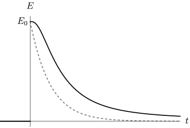
fig:energy

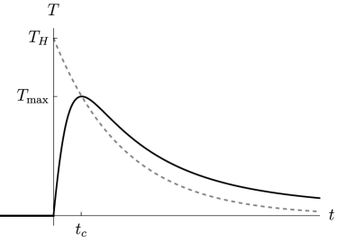
fig:temperature

Figure 1: For $A=0.5$, and $\kappa E_{0}=1$, the solid curves represent the black hole energy (a) and the black hole temperature (b) under the vacuum conditions $\Omega_{u}(t)=(1/2)\log\dot{\tau}(t)$ and $\Omega_{v}(t)=0$, while the dashed curves represent the results when $\Omega_{u}-\Omega_{v}$ is constant. In Fig. (a), the black hole energy is discontinuous at $t=0$ due to the shock wave. In Fig. (b), the black hole temperature described by the solid curve is continuous at $t=0$ and the maximum temperature occurs at a critical time $t_{c}$.

Next, the net flux thrown into the spacetime is obtained by differentiating the black hole energy (LABEL:eq:bdy_stress_tensor_in_evap) with respect to the boundary time as

$$\label{eq:diffbdystresstensor}\derivative{E}{t}=-\frac{\kappa N}{12\pi}E_{0}e^{-At}\left(\frac{I_{1}(\alpha)K_{1}(\alpha e^{-\frac{1}{2}At})-K_{1}(\alpha)I_{1}(\alpha e^{-\frac{1}{2}At})}{I_{1}(\alpha)K_{0}(\alpha e^{-\frac{1}{2}At})+K_{1}(\alpha)I_{0}(\alpha e^{-\frac{1}{2}At})}\right)^{2},$$ (52)

and the Stefan-Boltzmann law (LABEL:eq:Stefan-Boltzmann) leads to the black hole temperature for $t>0$

$$\label{eq:temperature}T(t)=T_{\rm H}e^{-\frac{1}{2}At}\left(\frac{I_{1}(\alpha)K_{1}(\alpha e^{-\frac{1}{2}At})-K_{1}(\alpha)I_{1}(\alpha e^{-\frac{1}{2}At})}{I_{1}(\alpha)K_{0}(\alpha e^{-\frac{1}{2}At})+K_{1}(\alpha)I_{0}(\alpha e^{-\frac{1}{2}At})}\right),$$ (53)

where $T(0)=0$, $\dot{T}(0)=\kappa E_{0}$ which is finite, and $T_{\rm H}$ is the Hawking temperature.

As shown in Fig. LABEL:fig:temperature, our calculations for the black hole temperature is zero for $t<0$ and the maximum value of it occurs when $t_{c}=\frac{2}{A}\log\frac{T_{\rm H}}{T_{\rm max}}$, where $T_{\rm max}=T(t_{c})$ and $\frac{dT}{dt}|_{t=t_{c}}=0$. The maximum temperature cannot exceed the Hawking temperature in the evaporating black hole. The black hole temperature starts from zero just when it is formed by the infalling shock wave. It then increases and reaches its maximum temperature at a finite time before gradually decreasing. The temperature profile after $t_{c}$ is compatible with the previous result in Ref. Engelsoy:2016xyb . However, the different solutions to vacuum conditions (LABEL:def:evap_cond) for the second term in Eq. (LABEL:eq:bdy_stress_tensor_wrt_tau) renders the earlier stage of the temperature profile different from the previous one.

V discussion

Using the dynamical boundary equation of motion proposed in Ref. Engelsoy:2016xyb , we obtained the holographic energy and temperature for the exactly soluble dynamical AdS₂ black holes by taking into account quantum backreaction. To ensure the validity of the energy expression (LABEL:eq:bdy_stress_tensor_wrt_tau), we first investigated the black hole in the Hartle-Hawking vacuum state and confirmed that its energy and temperature were compatible with those of the previous work. In the evaporating black hole of our main interest, we calculated the energy for the black hole in the Unruh vacuum state. Consequently, we found that at the very early stage of evaporation of the black hole, it is decaying slowly compared to the previous result so that the temperature proportional to the decay rate of the black hole energy starts from zero temperature. The temperature increases and reaches a peak at the critical time, and then vanishes eventually. In addition, the peak temperature never exceeds the Hawking temperature during evaporation.

Regarding the temperature behaviour mentioned above, the vanishing initial temperature and the existence of the upper bound may not be the first time. For example, in the RST model Russo:1992ax , the black hole temperature $T(\sigma^{-})=T_{\rm H}[1-(1+\frac{M}{\lambda}e^{\lambda(\sigma^{-}-\sigma_{0}^{+})})^{-2}]^{1/2}$ at future infinity Liberati:1994za ; Eune:2014tma starts from zero temperature initially and increases according to the monotonically increasing Hawking radiation, eventually vanishing after emission of the thunderpop energy. In this case, the maximum temperature during evaporation does not exceed the Hawking temperature: $T_{\rm max}(\sigma_{\rm s}^{-})=T_{\rm H}[1-e^{-\frac{96M}{N\lambda}}]^{1/2}$ Kim:1995wr , where $\sigma_{s}^{-}$ is the conformal time just before the black hole is completely evaporated.

In our work, the temperature of the black hole is assumed to be quasi-static, and thus the thermal bath can be maintained at the same temperature as the black hole. The black hole temperature vanishes at $t=0$, which means that the black hole has not yet emitted Hawking radiation to the bath at that instant. If the thermal effect of the black hole originates from pair creation around the black hole, then it may take a finite amount of time to thermalize, similar to the Hayden-Preskill protocol Hayden:2007cs .

A final comment is in order. The Page curve in the evaporating AdS₂ black hole Almheiri:2019psf shows that the entanglement entropy for the black hole and radiation system is increasing before the Page time and then decreasing after the Page time. In our temperature calculations, the maximal thermal temperature appears during the evaporation of the black hole at the critical time. It would be interesting to investigate whether there exists a correlation between the critical time for the maximum temperature and the Page time, in the context of the information loss paradox.

sec:conclusion

- (1) R. Jackiw, Lower Dimensional Gravity, Nucl. Phys. B 252 (1985) 343.
- (2) C. Teitelboim, Gravitation and Hamiltonian Structure in Two Space-Time Dimensions, Phys. Lett. B 126 (1983) 41.
- (3) J.M. Maldacena, J. Michelson and A. Strominger, Anti-de Sitter fragmentation, JHEP 02 (1999) 011 [hep-th/9812073].
- (4) A. Strominger, AdS(2) quantum gravity and string theory, JHEP 01 (1999) 007 [hep-th/9809027].
- (5) A. Almheiri and J. Polchinski, Models of AdS2 backreaction and holography, JHEP 11 (2015) 014 [1402.6334].
- (6) J.B. Hartle and S.W. Hawking, Path Integral Derivation of Black Hole Radiance, Phys. Rev. D 13 (1976) 2188.
- (7) W. Israel, Thermo field dynamics of black holes, Phys. Lett. A 57 (1976) 107.
- (8) J. Maldacena, D. Stanford and Z. Yang, Conformal symmetry and its breaking in two dimensional Nearly Anti-de-Sitter space, PTEP 2016 (2016) 12C104 [1606.01857].
- (9) W.G. Unruh, Notes on black hole evaporation, Phys. Rev. D 14 (1976) 870.
- (10) J. Engelsöy, T.G. Mertens and H. Verlinde, An investigation of AdS2 backreaction and holography, JHEP 07 (2016) 139 [1606.03438].
- (11) C.G. Callan, Jr., S.B. Giddings, J.A. Harvey and A. Strominger, Evanescent black holes, Phys. Rev. D 45 (1992) R1005 [hep-th/9111056].
- (12) S.B. Giddings and W.M. Nelson, Quantum emission from two-dimensional black holes, Phys. Rev. D 46 (1992) 2486 [hep-th/9204072].
- (13) J.G. Russo, L. Susskind and L. Thorlacius, The Endpoint of Hawking radiation, Phys. Rev. D 46 (1992) 3444 [hep-th/9206070].
- (14) E. Keski-Vakkuri and S.D. Mathur, Evaporating black holes and entropy, Phys. Rev. D 50 (1994) 917 [hep-th/9312194].
- (15) S. Liberati, A Real decoupling ghosts quantization of CGHS model for two-dimensional black holes, Phys. Rev. D 51 (1995) 1710 [hep-th/9407002].
- (16) J. Navarro-Salas, M. Navarro and C.F. Talavera, Weyl invariance and black hole evaporation, Phys. Lett. B 356 (1995) 217 [hep-th/9505139].
- (17) A. Fabbri and J.G. Russo, Soluble models in 2-d dilaton gravity, Phys. Rev. D 53 (1996) 6995 [hep-th/9510109].
- (18) S. Bose, L. Parker and Y. Peleg, Hawking radiation and unitary evolution, Phys. Rev. Lett. 76 (1996) 861 [gr-qc/9508027].
- (19) S. Nojiri and S.D. Odintsov, Trace anomaly induced effective action for 2-D and 4-D dilaton coupled scalars, Phys. Rev. D 57 (1998) 2363 [hep-th/9706143].
- (20) W.T. Kim, AdS(2) and quantum stability in the CGHS model, Phys. Rev. D 60 (1999) 024011 [hep-th/9810055].
- (21) M. Spradlin and A. Strominger, Vacuum states for AdS(2) black holes, JHEP 11 (1999) 021 [hep-th/9904143].
- (22) A. Fabbri and J. Navarro-Salas, Modeling black hole evaporation (2005).
- (23) A. Almheiri, N. Engelhardt, D. Marolf and H. Maxfield, The entropy of bulk quantum fields and the entanglement wedge of an evaporating black hole, JHEP 12 (2019) 063 [1905.08762].
- (24) P. Hayden and J. Preskill, Black holes as mirrors: Quantum information in random subsystems, JHEP 09 (2007) 120 [0708.4025].
- (25) A.M. Polyakov, Quantum Geometry of Bosonic Strings, Phys. Lett. B 103 (1981) 207.
- (26) D.V. Vassilevich, Heat kernel expansion: User’s manual, Phys. Rept. 388 (2003) 279 [hep-th/0306138].
- (27) Z. Yang, The Quantum Gravity Dynamics of Near Extremal Black Holes, JHEP 05 (2019) 205 [1809.08647].
- (28) T.G. Mertens and G.J. Turiaci, Solvable models of quantum black holes: a review on Jackiw–Teitelboim gravity, Living Rev. Rel. 26 (2023) 4 [2210.10846].
- (29) A. Strominger, Les Houches lectures on black holes, in NATO Advanced Study Institute: Les Houches Summer School, Session 62: Fluctuating Geometries in Statistical Mechanics and Field Theory, 8, 1994 [hep-th/9501071].
- (30) V. Balasubramanian and P. Kraus, A Stress tensor for Anti-de Sitter gravity, Commun. Math. Phys. 208 (1999) 413 [hep-th/9902121].
- (31) J. Engelsöy, Considerations regarding ads2 backreaction and holography, Master’s thesis, KTH, Physics, 2016.
- (32) J.F. Pedraza, A. Svesko, W. Sybesma and M.R. Visser, Semi-classical thermodynamics of quantum extremal surfaces in Jackiw-Teitelboim gravity, JHEP 12 (2021) 134 [2107.10358].
- (33) P.T. Landsberg and A.D. Vos, The stefan-boltzmann constant in n-dimensional space, Journal of Physics A: Mathematical and General 22 (1989) 1073.
- (34) M. Eune, Y. Gim and W. Kim, Note on explicit form of entanglement entropy in the Russo-Susskind-Thorlacius model, Phys. Rev. D 89 (2014) 127501 [1401.0590].
- (35) W.T. Kim and J. Lee, Hawking radiation and energy conservation in an evaporating black hole, Phys. Rev. D 52 (1995) 2232 [hep-th/9502115].