IR-finite thermal acceleration radiation

Abstract

A charge accelerating in a straight line following the Schwarzschild-Planck moving mirror motion emits thermal radiation for a finite period. Such a mirror motion demonstrates quantum purity and serves as a direct analogy of a black hole with unitary evolution and complete evaporation. Extending the analog to classical electron motion, we derive the emission spectrum, power radiated, and finite total energy and particle count, with particular attention to the thermal radiation limit. This potentially opens the possibility of a laboratory analog of black hole evaporation.

I Introduction

The precise metric solution to Einstein’s field equations in general relativity, unveiled by Schwarzschild Schwarzschild (1916), implied the existence of gravitationally collapsed stars that emit no light. Hawking proposed a semi-classical approximation Hawking (1974), using a quantum field subject to the classical background of the Schwarzschild metric, to show that black holes radiate with a thermal spectrum and temperature proportional to their surface gravity.

However, this discovery presented an obstacle, as the projected number of particles and radiated energy was infinite Hawking (1975), and Hawking’s computation scaled distances smaller than the Planck length Jacobson (1991), where the semi-classical approximation fails due to backreaction Fabbri and Navarro-Salas (2005), known as the trans-Planckian problem Brandenberger (2010). It appears unlikely that any direct observational confirmation of black hole evaporation will emerge Wald (2001), given the weakness of the anticipated amplitude relative to the interference from cosmic microwave background Parker and Toms (2009). Consequently, to date there is no astrophysical evidence for Hawking radiation.

A semi-classical approximation, using a quantum field subject to the classical trajectory of an accelerated mirror Fulling and Davies (1976) was also proposed by Davies-Fulling. This perfectly reflecting boundary DeWitt (1975) propagates through flat spacetime, a dynamical Casimir effect, radiating with a thermal spectrum and temperature proportional to acceleration Davies and Fulling (1977) in analogy to black hole radiation. A Schwarzschild mirror trajectory Good et al. (2016) exactly recreates the radiation emitted by a null shell collapse to a Schwarzschild black hole Wilczek (1993), including the aforementioned difficulties with infinite energy and particles Good (2018); Cong et al. (2019); Good (2016). A modified Schwarzschild trajectory for an accelerated mirror Good et al. (2020a) resolves the infinite radiation challenges of the Schwarzschild trajectory by limiting the acceleration via the introduction of a small length scale. The corresponding spacetime metric was obtained as a regularized form of the Schwarzschild spacetime called the Schwarzschild-Planck metric Good and Linder (2021); see also its closely related optical analog Moreno-Ruiz and Bermudez (2022). The accelerated equation of motion itself called the Schwarzschild-Planck trajectory is a globally defined, timelike, asymptotically zero velocity straight-line path in Minkowski spacetime.

The flat-spacetime simplicity and lower dimensions of the moving mirror model facilitate tractability in finding analytic Bogolyubov coefficients to investigate quantum particle creation Birrell and Davies (1984), as well as other quantities of interest like entanglement entropy Reyes (2021); Akal et al. (2021); Holzhey et al. (1994); Lee and Yeh (2019); Bianchi and Smerlak (2014), particle count Walker (1985a), and radiated energy Walker (1985b). In fact, Ford-Vilenkin Ford and Vilenkin (1982), Nikoshov-Ritus Nikishov and Ritus (1995), Zhakenuly et al. Zhakenuly et al. (2021), Ritus Ritus (1998, 2002, 2003), and others have exploited this simplicity to find powerful analogies between the classical radiation of an electron and the quantum radiation of a mirror. Indeed, a functional identity Ritus (2022), up to a pre-factor of $4\pi$ times the fine structure constant, exists between the electron and mirror. Moreover, this duality Good and Davies (2023) has made it possible to classically derive the Planck distribution connection between acceleration and temperature for an electron’s Larmor radiation Ievlev and Good (2023).

This work aims to investigate the classical Larmor radiation emitted by an electron traveling along the Schwarzschild-Planck trajectory to gain a better understanding of the thermal emission process usually associated with uniform proper acceleration and quantum radiation of the Davies-Fulling-Unruh effect Fulling (1973); Davies (1975); Unruh (1976). The advantages and novelty of the classical approach are the conceptual simplicity and analytic tractability of the thermal physics of radiation and the associated analog to complete black hole evaporation.

The paper is organized as follows. In Sec. II we introduce the Schwarzschild-Planck trajectory, focusing on its dynamics. In Sec. III and Sec. IV we compute the finite energy emitted by the electron, and the spectral-power distributions. Sec. V is devoted to thermality, asymptotic limits and finite particle production. Sec. VI reviews some background with respect to the generalized correspondence between mirrors and electrons; refining the recipe for the duality. Finally, Sec. VII and Sec. VIII end with remarks and conclusions.

II Schwarzschild-Planck trajectory

The Schwarzschild-Planck trajectory of the quantum pure mirror Good et al. (2020a) is

$$t(z)=-z-\frac{1}{g}\sinh 2\kappa z\ ,$$ (1)

where $\kappa$ and $g$ are two inverse length scales or accelerations. This was shown to correspond to the Schwarzschild-Planck black hole solution that evaporates without a remnant and preserves unitarity Good and Linder (2021). The idea is that one length scale $\kappa^{-1}$ would correspond to the Schwarzschild radius or black hole mass, and the other length scale $g^{-1}$ would be related in some way to the Planck scale. For our purposes here we regard $\kappa$ and $g$ as two parameters in an accelerated electron motion.

The velocity

$$V(z)\equiv\derivative{z}{t}=\frac{-g}{g+2\kappa\cosh 2\kappa z}\ ,$$ (2)

is zero in the limits $z\to\pm\infty$ and hence the motion is asymptotically static; see e.g.  Walker and Davies (1982), and also the two trajectories in Good and Linder (2023). This is critical for finite energy and particle production, and unitarity, and the relation between classical Larmor power and quantum Bogolyubov coefficients, as discussed in Ievlev and Good (2023); Good and Linder (2023). The maximum velocity $V_{\rm max}=-(1+2\kappa/g)^{-1}$ occurs at $z=0$ and approaches the speed of light for $\kappa/g\ll 1$.

II.1 Accelerations

The proper acceleration $\alpha\equiv\gamma^{3}\ddot{z}$, a Lorentz invariant scalar Rindler (1977), is

$$\alpha=\frac{-\sqrt{g\kappa}\,\sinh 2\kappa z}{2\,[\cosh 2\kappa z+(\kappa/g)\cosh^{2}2\kappa z]^{3/2}}\ ,$$ (3)

where $\gamma$ is the Lorentz boost factor. The acceleration vanishes asymptotically as $e^{-4\kappa|z|}\sim t^{-2}$.

Another useful quantity is the “local” or peel acceleration. Consider the acceleration Carlitz and Willey (1987a),

$$\bar{\kappa}=\frac{v^{\prime\prime}(u)}{v^{\prime}(u)}=2\alpha e^{\eta}=2\eta^{\prime}(u)\,,$$ (4)

where $\eta=\tanh^{-1}V$ is the rapidity, $v=t+z$ is advanced time, $u=t-z$ is retarded time, and $\alpha$ is the proper acceleration. Eq. (4) is called the ‘peel’, whose name has precedent in studies on the asymptotic behavior of zero-rest mass fields, see e.g.  Penrose Penrose (1965).

The peel acceleration function itself was perhaps first introduced as the local acceleration in Carlitz and Willey (1987a), and known from gravitational contexts as the peeling function, e.g. Bianchi and Smerlak (2014); Barcelo et al. (2011). In the electron radiation context Ievlev and Good (2023); Good (2023); Good and Davies (2023), the peel has also been associated with thermality. Interestingly, and surprisingly unlike the uniform proper acceleration of Unruh temperature Unruh (1976), the peel $\bar{\kappa}$ is the dynamic object that exhibits uniformity instead of the Lorentz invariant $\alpha$. The accelerating electron (or flying mirror) emits photons distributed in a Planck distribution with radiation temperature $T=\bar{\kappa}/2\pi$, not $T=\alpha/2\pi$.

Explicitly written using the Schwarzschild-Planck trajectory, Eq. (1), this object is

$$\bar{\kappa}=-\frac{\kappa\tanh 2\kappa z}{(r\cosh 2\kappa z+1)^{2}}\ ,$$ (5)

where $r=\kappa/g$. See Figure 1 for a plot of this acceleration. A key feature is the horizontal leveling associated with steady-state equilibrium. Here we will see the peel exhibits uniformity in connection with an associated thermal Planck distribution. The leveling out demonstrates a very slow change in the peel, commensurate with radiation emission. During this time, the system is in thermodynamic equilibrium, typical of a quasi-static process Schroeder (2000).

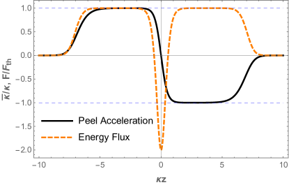
Figure 1: A plot of the peel acceleration, $\bar{\kappa}=2\alpha e^{\eta}=v^{\prime\prime}(u)/v^{\prime}(u)=2\eta^{\prime}(u)$. Here $g/\kappa=10^{6}$. A key takeaway is the leveling plateau indicative of steady-state equilibrium, which is in accordance with a Planck distribution of photons with temperature proportional to constant peel, $T=\kappa/2\pi$. For comparison, we show the energy flux, Eq. (6), radiated from a mirror with the same trajectory, also exhibiting a thermal plateau.

II.2 Energy Flux and Power

The energy flux $F$ of emitted radiation for the Schwarzschild-Planck case of a moving mirror can have a plateau at the thermal value $F_{\rm th}=\kappa^{2}/(48\pi)$, which lengthens as $\kappa/g\to 0$. Specifically, for $\kappa/g\ll 1$,

$$F(z)\approx F_{\rm th}\,\left[1-\frac{3}{\cosh^{2}2\kappa z}+{\mathcal{O}}\left(\frac{\kappa}{g}\right)\right]\ .$$ (6)

The thermal flux plateau lasts from $|\kappa z|\approx[1,(1/2)\ln(g/\kappa)]$. This corresponds to the period of uniform peel acceleration and equilibrium behavior. Note that $48\pi F(u)=\bar{\kappa}^{2}-2\bar{\kappa}^{\prime}$. See Good et al. (2020a) for a discussion of the necessary negative energy flux around $z=0$.

For simplicity, allow us to set $e=1$ in this section and the next. For a radiating charge, the Larmor power

$$P(z)=\frac{\alpha^{2}(z)}{6\pi}\ ,$$ (7)

is of interest, shown in Figure 2. Note that for tractability we express the power as a function of the spatial variable $z$ rather than the time variable $t$. Since the power dies off at large $z$ as $e^{-8\kappa z}$, or equivalently at large times as $t^{-4}$, we will obtain finite total energy.

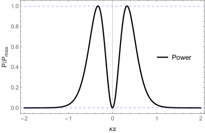
Figure 2: A plot of the Larmor power emitted by the electron, Eq. (7), $P=\alpha^{2}/6\pi$, normalized by its maximum value. A key takeaway is that the power is zero at the asymptotes, and the area under the curve, the total energy emitted, is finite. Here $g/\kappa=10^{6}$.

III Finite Energy

To compute the total energy of the quantum pure mirror (which is the same as the total energy radiated by the electron, see Ievlev and Good (2023)), we can integrate the Larmor power over all time to give

$$E = \frac{1}{6\pi}\int_{-\infty}^{\infty}dz\,\frac{dt}{dz}\,\alpha^{2}$$ (8)

$$= \frac{g^{3}}{24\pi}\int_{0}^{w}dw\,\frac{\sinh^{2}w}{\cosh^{3}w}\,\frac{g+2\kappa\cosh w}{(g+\kappa\cosh w)^{3}}\ ,$$ (9)

where $w=2\kappa z$, $r=\kappa/g$, and we have used the evenness of the integrand to change the interval from $[-\infty,+\infty]$ to $2\times[0,\infty]$.

This evaluates, with a continuous function across the three cases of $r>1$, $r=1$, $r<1$, to

$$E(r>1) = \frac{g}{24\pi}\,\left[\frac{\pi}{4}-\frac{r}{2(r^{2}-1)}\right.$$

$$\qquad\left.-\frac{r(2-r^{2})}{2(r^{2}-1)^{3/2}}\,\left(\sin^{-1}\frac{1}{r}-\frac{\pi}{2}\right)\right]$$

$$E(r=1) = \frac{\kappa(3\pi-8)}{288\pi}$$ (11)

$$E(r<1) = \frac{g}{24\pi}\,\left[\frac{\pi}{4}+\frac{r}{2(1-r^{2})}\right.-$$

$$\qquad\left.-\frac{r(2-r^{2})}{2(1-r^{2})^{3/2}}\,\ln\frac{1+\sqrt{1-r^{2}}}{r}\,\right]\ .$$

Limiting cases are $E(r\gg 1)=g^{3}/(192\kappa^{2})$ and $E(r\ll 1)=g/96$. Figure 3 plots the radiated total energy.

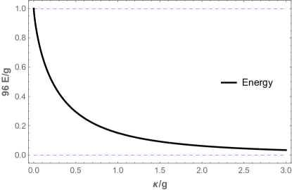
Figure 3: The total energy emitted by the electron, Eq. (9), is shown normalized to its value $g/96$ as $\kappa/g\to 0$. Notice the thermal regime corresponding to $g\gg\kappa$ has greater total energy emission while less energy is emitted in the non-thermal regime.

IV Distributions

IV.1 Spectral Distribution

The spectral distribution of the electron’s radiation is calculated with the help of the formula (see Jackson (1999) and also Eq. 26 of Ievlev and Good (2023))

$$\frac{\mathop{}\!\mathrm{d}I(\omega)}{\mathop{}\!\mathrm{d}\Omega}=\frac{\omega^{2}}{16\pi^{3}}\sin^{2}\theta\,\absolutevalue{j_{z}(\omega,k_{z})}^{2}\ ,$$ (13)

where $k_{z}=\omega\cos\theta$, and the Fourier transform of the current is defined as

$$j_{z}(\omega,k_{z}) =e\,\int\limits_{-\infty}^{\infty}\mathop{}\!\mathrm{d}{t}\,\derivative{z}{t}\,e^{-i(\omega t-k_{z}z(t))}$$ (14)

$$=e\,\int\limits_{-\infty}^{\infty}\mathop{}\!\mathrm{d}{z}\,e^{-i(\omega t(z)-k_{z}z)}\ .$$

Using the trajectory from Eq. (1) gives the spectral distribution

$$\frac{\mathop{}\!\mathrm{d}I}{\mathop{}\!\mathrm{d}\Omega}=\frac{e^{2}\omega^{2}\sin^{2}\theta}{16\pi^{3}\kappa^{2}}\,e^{-\frac{\pi\omega(1+\cos\theta)}{2\kappa}}\,\absolutevalue{K_{\frac{i\omega(1+\cos\theta)}{2\kappa}}\left(\frac{\omega}{g}\right)}^{2}\ ,$$ (15)

where $K$ is a modified Bessel function of the second kind.

Figure 4 plots this spectral distribution. Note the lack of emission in the $\theta=0$ direction and the strong emission in the transverse, $\theta=\pi/2$ direction. We also expect exponential suppression at high frequency. Integration over solid angle $\mathop{}\!\mathrm{d}{\Omega}=\sin\theta\mathop{}\!\mathrm{d}{\theta}\mathop{}\!\mathrm{d}{\phi}$ gives the spectrum $I(\omega)$, plotted in Figure 5.

Figure 4: The photon spectral distribution $\mathop{}\!\mathrm{d}{I}/\mathop{}\!\mathrm{d}{\Omega}=\mathop{}\!\mathrm{d}{E}/\mathop{}\!\mathrm{d}{\omega}\mathop{}\!\mathrm{d}{\Omega}$, Eq. (15), emitted by the electron moving downward with a Schwarzschild-Planck trajectory is shown, here for $\kappa=\omega=1$ and $g=100$.

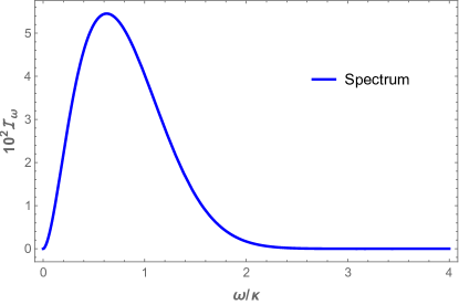
Figure 5: The photon spectrum $I(\omega)=\mathop{}\!\mathrm{d}{E}/\mathop{}\!\mathrm{d}{\omega}$ emitted by the electron moving along the Schwarzschild-Planck trajectory is shown for the same parameters as Fig. 4.

IV.2 Power Distribution

A key advantage of the classical approach is the analytic tractability of spacetime and spectral domains. For instance, the implicit time-dependent power distribution (computed as a function of $z$) is found using Eq. (1) with straightforward vector algebra Griffiths (2013) (see also e.g. the procedure in Good et al. (2019)),

$$\frac{\mathop{}\!\mathrm{d}{P}}{\mathop{}\!\mathrm{d}{\Omega}}=\frac{g^{4}\kappa^{4}\sin^{2}\theta\,\sinh^{2}2\kappa z}{\pi^{2}(g+2\kappa\cosh 2\kappa z)(g+g\cos\theta+2\kappa\cosh 2\kappa z)^{5}},$$ (16)

Figure 6 shows the power distribution $\mathop{}\!\mathrm{d}{P}/{\mathop{}\!\mathrm{d}{\Omega}}$. Its integration over solid angle $\mathop{}\!\mathrm{d}{\Omega}$ gives the Larmor power, Eq. (7). Further integration over time gives the total energy

$$E=\int\frac{\mathop{}\!\mathrm{d}{P}}{\mathop{}\!\mathrm{d}{\Omega}}\mathop{}\!\mathrm{d}{\Omega}\frac{\mathop{}\!\mathrm{d}{t}}{\mathop{}\!\mathrm{d}{z}}\mathop{}\!\mathrm{d}{z}\ .$$ (17)

Figure 6: The photon power distribution $\mathop{}\!\mathrm{d}{P}/\mathop{}\!\mathrm{d}{\Omega}=\mathop{}\!\mathrm{d}{E}/\mathop{}\!\mathrm{d}{t}\mathop{}\!\mathrm{d}{\Omega}$, Eq. (16), emitted by the electron moving downward with a Schwarzschild-Planck trajectory. Here $\kappa=1$ and $z=2$ (recall that $z$ defines a specific time $t$) and $g=100$.

V Thermality and asymptotic limits

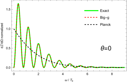
(a)

(b)

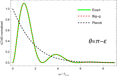
(c)

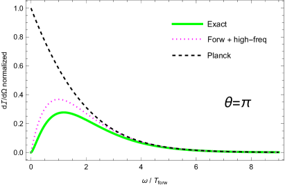
(d)

Figure 7: The spectral distribution, normalized as discussed in the text, is plotted for various directions $\theta$ of emission (as labeled in each panel), here for $g/\kappa=10^{10}$. Top left panel shows the backwards direction, top right is transverse to the motion, bottom right is exactly forwards, and bottom left is nearly but not exactly forwards ($\epsilon=50\sqrt{\kappa/g}=5\cdot 10^{-4}$). The thick green line is the result Eq. (15), the black dashed curve is the Planck factor Eq. (22), both normalized by a factor such that the Planck curve has the value 1 at the low-frequency asymptote. The red dashed line on panels (a)-(c) is the big-$g$ asymptotic Eq. (19), while the magenta dotted line on panel (d) represents the high-frequency, forward direction asymptotic Eq. (24). The spectral distribution away from the forward direction looks very similar at different angles when normalized and with the frequency axis scaled by a corresponding temperature $T_{\theta}$.

The spectral distribution Eq. (15) has a rich structure and here we consider various limiting cases and their relation to the Planck distribution denotes thermal equilibrium.

V.1 Planck Spectrum for Large $g$

Recall that the two length parameters entering the trajectory, $\kappa^{-1}$ and $g^{-1}$, were connected in the original Schwarzschild-Planck case to the black hole Schwarzschild radius (and hence mass) and the Planck length, respectively. In that case, we expect $g\gg\kappa$. In the present case there is an additional subtlety when considering the angular distribution in that $\kappa/(1+\cos\theta)$, not just $\kappa$, enters the spectral distribution.

We introduce the quantities

$$\kappa_{\theta}=\kappa\,\frac{2}{1+\cos\theta}\ ,\quad r_{\theta}=\frac{\kappa_{\theta}}{g}\ .$$ (18)

In the limit $r_{\theta}\ll 1$ the spectral distribution Eq. (15) reduces to a Planck form with oscillations,

$$\frac{1}{e^{2}\sin^{2}\theta}\frac{\mathop{}\!\mathrm{d}I}{\mathop{}\!\mathrm{d}\Omega}\Bigg{|}_{r_{\theta}\ll 1} = \frac{1}{8\pi^{2}\kappa(1+\cos\theta)}\,\frac{\omega}{e^{2\pi\omega/\kappa_{\theta}}-1}$$ (19)

$$\quad\times\left[1-\cos\varphi(\omega,\kappa_{\theta},g)\right]\ .$$

See Appendix A for the derivation. A far-away observer situated at an angle $\theta$ (where $\theta=0$ means the observer is behind the electron’s direction of motion) would see the temperature

$$T_{\theta}=\frac{\kappa_{\theta}}{2\pi}\ .$$ (20)

The phase

$$\varphi(\omega,\kappa_{\theta},g)=\frac{2\omega}{\kappa_{\theta}}\ln\frac{\omega}{2g}-2\operatorname{Arg}\left\{\Gamma(1+i\omega/\kappa_{\theta})\right\}$$ (21)

represents rapid oscillations (recall $r_{\theta}\ll 1$) with frequency $\sim(2/\kappa_{\theta})\ln(g/\kappa_{\theta})$. Note that $g$ only enters in the frequency of the oscillations, not their amplitude, which simply ranges over 0 to 2. The oscillations arise from the presence of a second length scale (i.e. $1/g$); see the discussion in Fernández-Silvestre et al. (2022) about their relation to interference effects between two effective horizons, even if the horizons don’t manifest physically. Averaging out the oscillations, we obtain a pure Planck distribution

$$\frac{1}{e^{2}\sin^{2}\theta}\frac{\mathop{}\!\mathrm{d}I}{\mathop{}\!\mathrm{d}\Omega}\Bigg{|}_{\begin{subarray}{c}r_{\theta}\ll 1\\[2.0pt] +\text{avg}\end{subarray}}\approx\frac{1}{8\pi^{2}\kappa(1+\cos\theta)}\,\frac{\omega}{e^{\omega/T_{\theta}}-1}\ .$$ (22)

The appearance of the Planck factor is consistent with known results for the corresponding mirror Good et al. (2020b, a), see Sec. VI here for the electron-mirror dictionary.

Figure 7 plots the spectral distribution, normalized by $e^{2}\sin^{2}\theta/[8\pi^{3}(1+\cos\theta)^{2}]$, as well as a Planck distribution with temperature $T_{\theta}$, normalized the same way.

For example, the limit $\theta\sim 0$ (where the observer is behind the electron, seeing it redshift as it recedes) gives the temperature $T_{0}=\kappa/2\pi$, see Fig. 7a. An “orthogonal” observer at $\theta=\pi/2$ would see the electron twice as hot, $T_{\pi/2}=\kappa/\pi$, see Fig. 7b.

At big $g$ this approximation remains valid in a wide region of angles $\theta\in[0,\pi-\epsilon_{\star}]$, where $\epsilon_{\star}=O(\sqrt{\kappa/g})$, so that $r_{\theta}\ll 1$ stays valid. Throughout all of this range oscillations follow the smooth Planck curve, and their average is the Planck distribution.

In a narrow region close to the forward direction $(\pi-\theta)\lesssim\kappa/g$, the condition $r_{\theta}\ll 1$ no longer holds. The oscillations become increasingly spread out, and the averaging to thermal gets steadily worse, see Fig. 7c. We treat this forward region next.

V.2 Wien’s Law in the Blueshift-Forward Limit

When $\theta\sim\pi$ (the observer is in front of the electron), the Bessel function in Eq. (15) reduces to $K_{0}$, giving

$$\frac{1}{e^{2}\sin^{2}\theta}\frac{\mathop{}\!\mathrm{d}I}{\mathop{}\!\mathrm{d}\Omega}\Bigg{|}_{\text{forw}}\approx\frac{\omega^{2}}{16\pi^{3}\kappa^{2}}\ \absolutevalue{K_{0}\left(\frac{\omega}{g}\right)}^{2}$$ (23)

In this case, a high-frequency asymptotic $\omega\gg g$ can be easily found,

$$\frac{1}{e^{2}\sin^{2}\theta}\frac{\mathop{}\!\mathrm{d}I}{\mathop{}\!\mathrm{d}\Omega}\Bigg{|}_{\begin{subarray}{c}\text{high-freq}\\[2.0pt] +\text{forw}\end{subarray}}\approx\frac{g}{32\pi^{2}\kappa^{2}}\ \omega e^{-\omega/T_{\text{forw}}}\ ,$$ (24)

where $T_{\text{forw}}=g/2$. This equation is Wien’s law with the temperature $T_{\text{forw}}$ (without oscillations). However, there is no Planck factor, so one can call this regime “thermal” only in a high-frequency sense, see Fig. 7d.

If the angle $\theta$ is not quite at zero, the formula for the temperature $T_{\text{forw}}$ receives corrections, see Eq. (54) and Fig. 9.

V.3 Infrared Limit

At low frequencies $\omega\to 0$ the spectral distribution Eq. (15) has an asymptotic form

$$\frac{\mathop{}\!\mathrm{d}I(\omega)}{\mathop{}\!\mathrm{d}\Omega}\approx\frac{e^{2}\omega^{2}\sin^{2}\theta}{16\kappa^{2}\pi^{3}}\left(\ln\frac{\omega}{2g}+\gamma\right)^{2}\ ,$$ (25)

where $\gamma$ is the Euler–Mascheroni constant (see Appendix A for the details). Note that the exact spectral distribution vanishes as $\omega\to 0$, and one should use the averaged formula Eq. (22) with care in the IR. A vanishing spectrum in the IR leads to finite particles, which will be computed in the following section.

V.4 Finite Particles

The single electron moving along the Schwarzschild-Planck trajectory radiates a finite number of photons. The particle spectrum $\mathop{}\!\mathrm{d}{N}_{\gamma}(\omega)/\mathop{}\!\mathrm{d}{\omega}$ is, using Eq. (15),

$$\frac{\mathop{}\!\mathrm{d}{N}_{\gamma}}{\mathop{}\!\mathrm{d}{\omega}}=\int\frac{1}{\omega}\frac{\mathop{}\!\mathrm{d}{I}}{\mathop{}\!\mathrm{d}{\Omega}}\mathop{}\!\mathrm{d}{\Omega}\ .$$ (26)

Integrating over all the frequencies $\omega$ gives the total number of photons emitted $N_{\gamma}$,

$$N_{\gamma}=\int_{0}^{\infty}\int_{0}^{2\pi}\int_{0}^{\pi}\frac{1}{\omega}\frac{\mathop{}\!\mathrm{d}{I}}{\mathop{}\!\mathrm{d}{\Omega}}\sin\theta\mathop{}\!\mathrm{d}{\theta}\mathop{}\!\mathrm{d}{\phi}\mathop{}\!\mathrm{d}{\omega}\ .$$ (27)

Figure 8 plots the total particle count as a function of $g/\kappa$. This is a key difference between the two types of asymptotic inertial motions: the finite particle count of asymptotically zero-velocity trajectories is a signature property in contrast to the infinite soft particle production of asymptotically non-zero sub-light velocity trajectories. We note that finite energy, entropy, and particle count are useful qualities for correspondence with realistic experiments and unitary physical conditions.

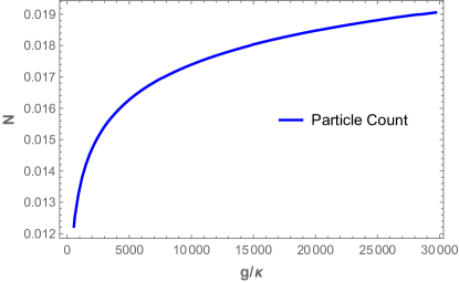
Figure 8: Photon count, Eq. (27), emitted by the electron moving along the Schwarzschild-Planck trajectory is plotted vs $g/\kappa$. Recall that $N_{\gamma}\propto e^{2}=4\pi\alpha_{\textrm{fs}}\approx 0.092$, in units where $\hbar=c=\epsilon_{0}=\mu_{0}=1$.

VI Radiant electron-mirror correspondence

We now return to the connection between classical electrodynamics (a point charge moving in 3+1d) and quantum field theory (dynamical boundary condition for a scalar field in 1+1d).

Let us start with reviewing some background regarding this correspondence (see e.g. Birrell and Davies (1984)). In the moving mirror setup, we consider a massless scalar field in 1+1-dimensional spacetime DeWitt (1975); Fulling and Davies (1976); Davies and Fulling (1977). If the spacetime were actually Minkowski, the vacuum is trivial, and in the absence of sources, there is no radiation. However, a moving mirror is a dynamical boundary condition Good et al. (2021), and this causes perturbation of the vacuum and creation of scalar field quanta, as the dynamical Casimir effect. An observer sees this as radiation.

The total energy radiated as a result of this dynamical Casimir effect is (see e.g. Walker (1985a))

$$E_{\text{tot}}^{\beta}=\int\limits_{0}^{\infty}dp\int\limits_{0}^{\infty}dq\ p\;|\beta_{pq}|^{2}\ .$$ (28)

Here $|\beta_{pq}|^{2}=|\beta^{R}_{pq}|^{2}+|\beta^{L}_{pq}|^{2}$, and $\beta^{R,L}_{pq}$ are the beta Bogolyubov coefficients for the right and left sides of the mirror Parker and Toms (2009) (see also Zhakenuly et al. (2021); Good et al. (2022); Good and Ong (2023)). Frequencies $p$ and $q$ refer to outgoing and incoming plane waves, see e.g. Fabbri and Navarro-Salas (2005).

VI.1 Short Review of Previous Results

Following Nikishov-Ritus Nikishov and Ritus (1995) (see also Ritus (1998, 2002, 2003, 2022)), the authors of Ievlev and Good (2023); Good and Linder (2023) related the beta Bogolyubov coefficients $|\beta_{pq}|^{2}$ to a certain Lorentz scalar characteristic of the electron moving in 3+1d. The formula stated in Ievlev and Good (2023) is

$$\frac{|j_{\mu}(\omega,k_{z})|^{2}+|j_{\mu}(-\omega,k_{z})|^{2}}{(2\pi)^{2}e^{2}}=|\beta_{pq}|^{2}\ ,$$ (29)

(note that $|j_{\mu}(-\omega,k_{z})|^{2}=|j_{\mu}(\omega,-k_{z})|^{2}$) where $2p=\omega+k_{z}$, $2q=\omega-k_{z}$, and the scalar $|j_{\mu}(\omega,k_{z})|^{2}$ is defined as

$$|j_{\mu}(\omega,k_{z})|^{2}\equiv|\bm{j}(\omega,k_{z})|^{2}-|\rho(\omega,k_{z})|^{2}\ .$$ (30)

Here $\bm{j}$ and $\rho$ are the Fourier-transformed three-current and charge density. The correspondence propagates to the total energy radiated by an electron through the equivalence Ievlev and Good (2023); Good and Linder (2023) of

$$E_{\text{tot}}^{e} =\int\limits_{0}^{\infty}d\omega\int d\Omega\,\frac{\mathop{}\!\mathrm{d}I(\omega)}{\mathop{}\!\mathrm{d}\Omega}\ ,$$ (31)

and the total energy of radiation coming from a mirror that moves on the same trajectory,

$$E_{\text{tot}}^{\beta}=\int\limits_{0}^{\infty}dp\int\limits_{0}^{\infty}dq\ p\;|\beta_{pq}|^{2}\ .$$ (32)

VI.2 Refined Recipe Derivation

Now we derive a more refined version of this correspondence, given a full derivation of Eq. (29) as opposed to the previous more heuristic motivation (and check of the final result).

We begin by writing down the formula for the beta Bogolyubov coefficients. For the right side of the mirror, (see Eq. 2.23 of Good et al. (2013), Eqs. 77-80 of Good et al. (2017), or Fabbri and Navarro-Salas (2005); Birrell and Davies (1984)),

$$\beta_{pq}^{R}=\frac{1}{4\pi\sqrt{pq}}\int\limits_{-\infty}^{v_{0}}\mathop{}\!\mathrm{d}v\,e^{-iqv-ipf(v)}\left(q-p\,\derivative{f(v)}{v}\right)\ .$$ (33)

In this equation, the mirror’s trajectory is defined as $u=f(v)$ in terms of the lightcone coordinates

$$u=t-z\,,\quad v=t+z\ .$$ (34)

This is equivalent to defining the trajectory in the form $z=z(t)$. Here $v_{0}$ is the position of the mirror’s horizon; for a mirror without a horizon (like the Schwarzschild-Planck case we focus on in this paper) one should set $v_{0}=\infty$.

Making a change of variables in Eq. (33) we pass from integration over $v$ to the integration over $t$ according to

$$u=t-z(t)\ ,\quad v=t+z(t)\ .$$ (35)

Moreover, we substitute the frequencies $p,q$ by the electron-related frequency as

$$p+q=\omega\,,\quad p-q=\omega\cos\theta\ .$$ (36)

The ingredients of Eq. (33) become under this transformation

$$\mathop{}\!\mathrm{d}v =(\dot{z}(t)+1)\mathop{}\!\mathrm{d}t\ ,$$ (37)

$$q-p\frac{df(v)}{dv} =\omega\,\frac{\dot{z}(t)-\cos\theta}{\dot{z}(t)+1}\ ,$$

$$qv+pf(v) =\omega\,(t-z(t)\,\cos\theta)\ .$$

Now we can easily write down a transformed version of Eq. (33):

$$\beta_{pq}^{R} =\frac{1}{2\pi\sin\theta}\int\limits_{-\infty}^{\infty}\mathop{}\!\mathrm{d}t\,(\dot{z}(t)-\cos\theta)\,e^{-i\omega(t-z\cos\theta)}$$

$$=\frac{1}{2\pi e\sin\theta}\,[j_{z}(\omega,\omega\cos\theta)-\rho(\omega,\omega\cos\theta)\cos\theta]\ .$$

where the charge and current densities are

$$\rho=e\,\delta(z-z(t))\,,\quad j_{z}=e\dot{z}\,\delta(z-z(t))\ .$$ (38)

Using the charge conservation law

$$\omega\rho(\omega,\bm{k})-\bm{k}\cdot\bm{j}(\omega,\bm{k})=0\ ,$$ (39)

we arrive at the final answer

$$\beta_{pq}^{R}=\frac{\sin\theta}{2\pi e}\ j_{z}(\omega,\omega\cos\theta)\ .$$ (40)

This gives a refined form of the correspondence.

The beta Bogolyubov coefficients for the left side of the mirror are related to the right side by a parity flip, $\beta^{L}_{pq}=\beta^{R}_{qp}$. One can repeat the derivation or realize the parity flip is equivalent to $\theta\to\pi-\theta$. Either way one easily obtains the previously stated correspondence Eq. (29) written for both sides of the mirror with $|\beta_{pq}|^{2}\equiv|\beta^{R}_{pq}|^{2}+|\beta^{L}_{pq}|^{2}$.

VI.3 Practical Significance

Although the newly derived correspondence is interesting and intriguing in and of itself, it also has a potential for applications. Taking the absolute value squared of Eq. (40) and comparing with Eq. (13) we can relate the mirror to the electron’s spectral distribution:

$$\frac{1}{e^{2}\omega^{2}}\,\frac{\mathop{}\!\mathrm{d}{I}}{\mathop{}\!\mathrm{d}{\Omega}}(\omega,\cos\theta) =\frac{1}{4\pi}|\beta^{R}_{pq}|^{2}\,,$$ (41)

$$p+q=\omega\,, p-q=\omega\cos\theta\,.$$

The l.h.s. contains only electron quantities, while the r.h.s. is in terms of mirror quantities. This formula allows one to convert between the radiation from an accelerating boundary (mirror) in 1+1d and an accelerating charge in 3+1d that move on the same rectilinear trajectory.

We explicitly checked for several trajectories that this correspondence indeed works. For example, take the beta Bogolyubov coefficients for the Schwarzschild-Planck mirror (see e.g. Eq. 7 of Good et al. (2020a) and Eq. 3 of Good et al. (2020b)):

$$|\beta_{pq}^{R}|^{2}=\frac{pq}{\pi^{2}\kappa^{2}(p+q)^{2}}\ e^{-\frac{\pi p}{\kappa}}\,\absolutevalue{K_{ip/\kappa}\left(\frac{p+q}{g}\right)}^{2}\ .$$ (42)

One can immediately see that the recipe Eq. (41) gives the spectral distribution Eq. (15).

For the total energy the correspondence of Eq. (41) agrees with the derivation of Good and Linder (2023); Ievlev and Good (2023) that the total energy radiated by an electron is equal to the total energy from both sides of the mirror, as can be seen by the following. Using the electron’s total radiated energy formula Eq. (31) and the correspondence Eq. (41) we obtain an expression for the total energy from the mirror,

$$E_{\text{tot}}^{\beta}=\int\limits_{0}^{\infty}dp\int\limits_{0}^{\infty}dq\ (p+q)\;|\beta^{R}_{pq}|^{2}\,.$$ (43)

Now recall that a parity flip relates the two sides of the mirror, so

$$E_{\text{tot}}^{\beta} =\int\limits_{0}^{\infty}dp\int\limits_{0}^{\infty}dq\ p\;|\beta^{R}_{pq}|^{2}+\int\limits_{0}^{\infty}dp\int\limits_{0}^{\infty}dq\ q\;|\beta^{R}_{pq}|^{2}$$ (44)

$$=\int\limits_{0}^{\infty}dp\int\limits_{0}^{\infty}dq\ p\;|\beta^{R}_{pq}|^{2}+\int\limits_{0}^{\infty}dp\int\limits_{0}^{\infty}dq\ q\;|\beta^{L}_{qp}|^{2}\,.$$

By relabeling the variables $q\leftrightarrow p$ in the last integral we immediately recover Eq. (28).

For convenience, we also provide Table 1 giving the correspondence between some mirror limits and electron limits. Recall that $p=\omega(1+\cos\theta)/2$, $q=\omega(1-\cos\theta)/2$.

Mirror	Electron
moves to the left	moves down $z\to-\infty$
high-freq. $q\gg p$	blueshift-forward $\theta\to\pi$, $q\approx\omega$
low-freq. $q\ll p$	redshift-recede $\theta\to 0$, $p\approx\omega$

Table 1: Correspondence between mirror and electron properties in various limits.

VII Other Remarks

VII.1 Resistors, accelerating electrons, and black holes

The one-channel Planck curve, Eq. (22), also appears as the signature form of Nyquist white noise Nyquist (1928) for a resistor. The noise power emitted by a resistor is independent of the resistance (see e.g. Eq. 15.17.14 of Reif Reif (1965)),

$$P(\omega)=\frac{\mathop{}\!\mathrm{d}{\omega}}{2\pi}\frac{\hbar\omega}{e^{\hbar\omega/k_{B}T}-1}\ ,$$ (45)

and equivalent to what an antenna would pick up from a three-dimensional black body at the same temperature Dicke (1946). Lowering the temperature means lower noise. This curve is essential to understanding and mitigating the impact of thermal noise on electronic systems at high frequencies or low temperatures, $\hbar\omega\gg k_{B}T$, due to quantum effects Urick et al. (2021). Thus, the one-channel Planck curve’s appearance in the classical radiation from an accelerating electron is remarkable. We note that as far as information flow is concerned, a black hole also behaves as a one-dimensional channel Bekenstein and Mayo (2001); Bekenstein (2003, 2002).

VII.2 Remarks on electron evaporation

Complete evaporation should address the problem of backreaction. A fixed background approximation ignores the effects of the radiation on the spacetime geometry. Backreaction effects are expected to play an important role even before reaching the Planck scale when the unknown theory of quantum gravity is expected to dominate Fabbri and Navarro-Salas (2005). The classical thermal Schwarzschild-Planck model of an accelerated electron is an analog for black hole radiance. The model goes beyond solving for the finite energy emission that is one of the primary consequences of backreaction but also results in finite particle emission, leaving no confusion about the end state of the black hole radiation process: complete evaporation with no left-over remnant Wilczek (1993).

In the context of quantum theory, an electron can never truly come to a complete stop without considering the uncertainty principle. At late times, the electron’s velocity, Eq. (2), becomes arbitrarily small,

$$\lim_{t\to\infty}V(t)=0\,,$$ (46)

as $1/(2\kappa t)$, and consequently, the wave function becomes more and more spread out over time, in a process not so different to ‘complete black hole evaporation’; i.e. crudely speaking, the black hole ‘spreads’ itself out over time. In other words, the de Broglie wavelength of such an electron becomes huge:

$$\lambda_{\text{dB}}=\frac{h}{p}\ ,$$ (47)

where $h$ is Planck’s constant and $p$ is the electron’s momentum. Supposing the wave function of the electron becomes infinitely spread out, its magnitude approaches zero, and the probability of finding the electron in a specific region of space becomes very small.

However, the radiation emitted by the point charge in this paper is completely classical. What are the signatures for classical complete evaporation? The mass of the black hole lessens, converting to radiation energy. The electron mass never changes. Nevertheless, the electron ‘goes away’ by traveling to asymptotic infinity, Eq. (1),

$$\lim_{t\to\infty}z(t)=-\infty\ .$$ (48)

This infinity is an important artifact of the model but is not unique to asymptotic zero-velocity motions. Consider numerous models, e.g. Good and Ong (2015), which are also asymptotic inertial but obtain asymptotic constant velocity,

$$\lim_{t\to\infty}V(t)=V_{0}=\textrm{constant}\ ,$$ (49)

with $1>|V_{0}|>0$. In this case, the de Broglie wavelength stays finite. These asymptotic constant velocity electrons may also travel to spatial infinity, yet they do not ‘go away’: a residual Doppler shift Wilczek (1993) and soft photons Ievlev and Good (2023) signal their eternal presence. How, then, can these classical considerations yield insight into complete evaporation? Consider how the measurement of velocity requires successive measures of position. If an electron is absent, there will be no measurable change in position, which a zero velocity measurement would reflect. Consider also that the IR limit $\omega\to 0$ of the classical spectrum $I(\omega)$ is zero for an asymptotically resting electron but non-zero for asymptotic drift.

VIII Conclusions

We have found conditions under which an accelerating electron emits thermal radiation. By using the Schwarzschild-Planck trajectory, thermality and asymptotic rest (hence finite particle and energy emission) are reconciled. Some key takeaways:

• A peel acceleration plateau demonstrates a steady-state dynamics connection to the thermal spectrum. The electron accelerates with uniform peel, leading to the emission of thermal radiation.

• There is a refined and precise ‘holographic’ duality between the radiation emitted by an accelerating electron in 3+1 dimensions and a moving mirror in 1+1 dimensions. This recipe explicitly connects the mirror’s Bogolyubov coefficients to the electron’s spectral distribution.

• The temperature arising from calculating the spectral distribution is explicitly related to the acceleration. The necessary two length scales of Schwarzschild-Planck give high-frequency oscillations about a Planck spectrum.

While this paper develops a fully classical radiation model, it establishes critical characteristics expected of complete black hole evaporation (with unitarity, i.e. no information loss). Several possible extensions related to black holes are of interest:

• A modified null-shell collapse could more closely link the properties of black hole radiation and electron radiation.

• A better understanding of the curved geometry associated with the Schwarzschild-Planck spacetime from the spectral insights gleaned here could help develop a geometric perspective of backreaction.

• Relaxing the strong constraint of asymptotic rest and investigating asymptotic drift could be an interesting direction, to see whether black hole remnants and asymptotic drifting electrons share radiated particle spectral signatures.

Closer to laboratory experiments, one might apply the fluctuation-dissipation theorem (FDT) to the thermal accelerating electron. The FDT has utilized the 1+1 Planck curve (Eq. 4.9 of Callen and Welton (1951)) to find the fluctuating voltage of a resistor and other canonical examples like the fluctuating force responsible for Brownian motion.

Appendix A Technical Details of the Asymptotic Expansions

In this Appendix we derive the asymptotic formulas presented in the main text, and also present some additional technical results.

The first step in this analysis is the asymptotic expansion of the modified Bessel function. We employ the following integral representation,

$$K_{i\omega/\kappa_{\theta}}\left(\frac{\omega}{g}\right) =\frac{1}{2}\int\limits_{-\infty}^{\infty}e^{-\omega f(z)}\,dz\ ,$$ (50)

$$f(z) =\frac{1}{g}\cosh z+\frac{i}{\kappa_{\theta}}z\ .$$

A.1 High-frequency limit

At high frequencies $\omega$ (i.e. roughly speaking $\omega\gg g$ or $\omega\gg\kappa_{\theta}$ – see below) one can apply the saddle-point method to the integral in Eq. (50). There are two cases depending on the value of the parameter $r_{\theta}=\kappa_{\theta}/g$.

When $r_{\theta}>1$, there is only one relevant saddle point: $z_{0}=-i\sin[-1](1/r_{\theta})$. The saddle point approximation works well if

$$\omega f^{\prime\prime}(z_{0})=\frac{\omega}{g}\sqrt{1-\frac{1}{r_{\theta}^{2}}}\ \gg 1\,,$$ (51)

and under this assumption one obtains

$$K_{i\omega/\kappa_{\theta}}\left(\omega/g\right) \approx\sqrt{\frac{\pi g}{2\omega\sqrt{1-1/r^{2}_{\theta}}}}$$ (52)

$$\times e^{-\frac{\omega}{g}\left[\sqrt{1-1/r_{\theta}^{2}}+(1/r_{\theta})\sin^{-1}(1/r_{\theta})\right]}\ .$$

Plugging this into the spectral distribution Eq. (15) gives Wien’s law

$$\frac{\mathop{}\!\mathrm{d}I}{\mathop{}\!\mathrm{d}\Omega} \approx\frac{e^{2}g\sin^{2}\theta}{32\pi^{2}\kappa^{2}\sqrt{1-1/r_{\theta}^{2}}}\cdot\omega\,e^{-\omega/T_{g}}\ ,$$ (53)

with temperature

$$T_{g}=\frac{g}{2}\left(\sqrt{1-\frac{1}{r_{\theta}^{2}}}+\frac{\pi-\cos[-1](1/r_{\theta})}{r_{\theta}}\right)^{-1}\,.$$ (54)

Blueshift-forward limit implies $r_{\theta}\to\infty$, $T_{g}\to g/2$, and we recover Eq. (24) in this limit.

At $r_{\theta}=1$ this saddle point merges with another saddle point, and a Stokes-like phenomenon occurs. In the interval $0<r_{\theta}<1$ two saddle points contribute to the integral in Eq. (50): $z_{\pm}=-i\pi/2\pm\ln(1/r_{\theta}-\sqrt{1/r_{\theta}^{2}-1})$. The saddle point approximation works well if

$$\omega\,\absolutevalue{f^{\prime\prime}(z_{\pm})}=\frac{\omega}{\kappa_{\theta}}\sqrt{1-r_{\theta}^{2}}\ \gg 1\,.$$ (55)

The appearance of two saddle points results in an oscillating asymptotic behavior:

$$K_{i\omega/\kappa_{\theta}}\left(\omega/g\right)\approx\sqrt{\frac{2\pi\kappa_{\theta}}{\omega\sqrt{1-r_{\theta}^{2}}}}\ \cos(\omega\Upsilon/2+\pi/4)\ e^{-\frac{\pi\omega}{2\kappa_{\theta}}}\,,$$ (56)

where the oscillation factor is

$$\Upsilon=\frac{2}{\kappa_{\theta}}\left[\sqrt{1-r_{\theta}^{2}}+g\ln(1/r_{\theta}-\sqrt{1/r_{\theta}^{2}-1})\right]\,.$$ (57)

Plugging this into the spectral distribution Eq. (15) gives Wien’s law

$$\frac{\mathop{}\!\mathrm{d}I}{\mathop{}\!\mathrm{d}\Omega} \approx\frac{e^{2}\sin^{2}\theta}{8\pi^{2}\kappa(1+\cos\theta)\sqrt{1-r_{\theta}^{2}}}$$ (58)

$$\times\left[1-\cos(\omega\Upsilon-\pi/2)\right]\cdot\omega\,e^{-\omega/T_{\theta}}\ ,$$

with temperature $T_{\theta}$ that exactly coincides with Eq. (20),

$$T_{\theta}=\frac{\kappa_{\theta}}{2\pi}\ .$$ (59)

In the limit of large $g$ we generally have $r_{\theta}\to 0$, and Eq. (58) reproduces a high-frequency approximation to the oscillating Planck distribution in Eq. (19). Using Stirling’s approximation, we checked that the phase Eq. (21) and the phase of $\cos$ in Eq. (58) also agree in the limit of large $g$. In the blueshift-forward limit $\theta=\pi$, then “large” $g$ may be small compared to $\kappa_{\theta}=\kappa/(1+\cos\theta)$ and so we no longer have the limit $r_{\theta}\to 0$. Thus the temperature in Eq. (59) does not actually blow up.

In fact, there is a smooth transition between the branches, with Eq. (54) and Eq. (59) giving the same result at $r_{\theta}=1$. The full behavior is shown in Fig. 9.

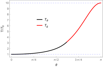
Figure 9: Temperature seen by a remote observer positioned at an angle $\theta$ (relevant formulas are Eq. 54 and Eq. 59). The temperature is plotted in units of $T_{0}=\kappa/2\pi$, and here $\kappa=2\pi$, $g=20$. The transition between the redshift-receding $\theta=0$ limit and the blueshift-forward $\theta=\pi$ limit is indeed smooth, and as expected the temperature rises in this transition.

A.2 Large-$g$ expansion

We start by analyzing the spectral distribution in the limit $\omega/g\ll 1$. The expansion of the modified Bessel function of the second kind is easy in this limit. Starting from its definition in terms of the modified Bessel function of the first kind,

$$K_{i\alpha}(x)=\frac{\pi}{2\sin(i\alpha\pi)}\left[I_{-i\alpha}(x)-I_{i\alpha}(x)\right]\,,$$ (60)

and using the expansion of the $I$-function at small arguments (see e.g. Gradshteyn & Ryzhik Eq. 8.445)

$$I_{i\alpha}(x)\approx\frac{1}{\Gamma(1+i\alpha)}\left(\frac{x}{2}\right)^{i\alpha}\,,\quad x\to 0$$ (61)

we can easily arrive at

$$K_{i\alpha}(x)\approx\frac{\pi}{2i\sinh(\pi\alpha)}\Big{[} \frac{1}{\Gamma(1-i\alpha)}\left(\frac{x}{2}\right)^{-i\alpha}$$ (62)

$$-\frac{1}{\Gamma(1+i\alpha)}\left(\frac{x}{2}\right)^{i\alpha}\Big{]}\ .$$

Next, using $|a-b|^{2}=|a|^{2}+|b|^{2}-2\real(a^{*}\cdot b)$ and the identity

$$\absolutevalue{\Gamma(1+i\alpha)}^{2}=\frac{\pi\alpha}{\sinh\pi\alpha}\ ,$$ (63)

we find

$$\absolutevalue{K_{i\alpha}(x)}^{2}=\frac{\pi}{2\alpha\sinh(\pi\alpha)}$$ (64)

$$\quad\times\Big{[}1-\cos(2\alpha\ln\frac{x}{2}-2\operatorname{Arg}(\Gamma(1+i\alpha)))\Big{]}\,.$$

Plugging this into the spectral distribution Eq. (15) with $x=\omega/g$, $\alpha=\omega/\kappa_{\theta}$ yields the formula Eq. (19).

Although we started this derivation under the assumption $\omega/g\ll 1$, the result actually remains valid at large $\omega$ if we have $r_{\theta}=\kappa_{\theta}/g\ll 1$. This conclusion is confirmed by the fact that the high-frequency asymptotic result Eq. (58) is consistent with the high-frequency limit of Eq. (19).

A.3 Low-frequency limit

If in addition to $\omega/g\ll 1$ we also assume $\omega/\kappa_{\theta}\ll 1$, we can get a simple IR asymptotic formula valid for all $\theta$.

In Eq. (64) take $\alpha\ll 1$. In this limit (see e.g. Gradshteyn & Ryzhik Eq. 8.342)

$$\ln\Gamma(1+i\alpha)\approx-i\gamma\alpha\,,$$ (65)

and we find $\operatorname{Arg}\Gamma(1+i\alpha)\approx-\gamma\alpha$. Here $\gamma$ is the Euler–Mascheroni constant. Then we can expand the $\cos$ and the $\sinh$ in Eq. (64) to obtain

$$\absolutevalue{K_{i\alpha}(x)}^{2}\approx\left(\ln\frac{x}{2}+\gamma\right)^{2}\ .$$ (66)

Plugging this with $\alpha=\omega/\kappa_{\theta}$ and $x=\omega/g$ into the spectral distribution Eq. (15) we obtain the IR result Eq. (25). We checked numerically that this approximation indeed works.

Appendix B Meaning of Large-$g$

In Sec. V we demonstrated that in the limit of large $g$ the electron’s spectral distribution acquires the Planck form Eq. (22), and we may speak of a thermal radiation at all frequencies. Here we briefly motivate the reason why large $g$ is significant.

Writing Eq. (1) in dimensionless form as

$$\kappa t=-\kappa z-\frac{\kappa}{g}\sinh 2\kappa z\,,$$ (67)

immediately shows that small $\kappa/g$ gives a longer period where the motion is near the speed of light, a requirement for getting mirror thermal radiation. Moreover, the approach to this behavior is exponential, $\sim e^{2\kappa z}$, which together yield thermal radiation (see Good and Linder (2018); Davies and Fulling (1977) and Carlitz-Willey Carlitz and Willey (1987b) for further discussion.)

Recall that in the original Schwarzschild-Planck mirror analysis Good and Linder (2021), the conjecture was that the new length scale was related to the Planck length, with $g\propto 1/l_{\rm Pl}$. Hence we indeed expect $g$ to be large compared to other scales.

References

- Schwarzschild (1916) K. Schwarzschild, On the gravitational field of a mass point according to Einstein’s theory, Sitzungsber. Preuss. Akad. Wiss. Berlin (Math. Phys. ) 1916, 189 (1916), arXiv:physics/9905030 .
- Hawking (1974) S. W. Hawking, Black hole explosions, Nature 248, 30 (1974).
- Hawking (1975) S. Hawking, Particle Creation by Black Holes, Commun. Math. Phys. 43, 199 (1975).
- Jacobson (1991) T. Jacobson, Black hole evaporation and ultrashort distances, Phys. Rev. D 44, 1731 (1991).
- Fabbri and Navarro-Salas (2005) A. Fabbri and J. Navarro-Salas, Modeling Black Hole Evaporation (Imperial College Press, 2005).
- Brandenberger (2010) R. H. Brandenberger, Introduction to Early Universe Cosmology, PoS ICFI2010, 001 (2010), arXiv:1103.2271 [astro-ph.CO] .
- Wald (2001) R. M. Wald, The thermodynamics of black holes, Living Rev. Rel. 4, 6 (2001), arXiv:gr-qc/9912119 .
- Parker and Toms (2009) L. E. Parker and D. Toms, Quantum Field Theory in Curved Spacetime: Quantized Field and Gravity, Cambridge Monographs on Mathematical Physics (Cambridge University Press, 2009).
- Fulling and Davies (1976) S. A. Fulling and P. C. W. Davies, Radiation from a moving mirror in two dimensional space-time: conformal anomaly, Proc. R. Soc. Lond. A 348, 393 (1976).
- DeWitt (1975) B. S. DeWitt, Quantum Field Theory in Curved Space-Time, Phys. Rept. 19, 295 (1975).
- Davies and Fulling (1977) P. Davies and S. Fulling, Radiation from Moving Mirrors and from Black Holes, Proc. R. Soc. Lond. A A356, 237 (1977).
- Good et al. (2016) M. R. R. Good, P. R. Anderson, and C. R. Evans, Mirror Reflections of a Black Hole, Phys. Rev. D 94, 065010 (2016), arXiv:1605.06635 [gr-qc] .
- Wilczek (1993) F. Wilczek, Quantum purity at a small price: Easing a black hole paradox, in International Symposium on Black holes, Membranes, Wormholes and Superstrings (1993) pp. 1–21, arXiv:hep-th/9302096 .
- Good (2018) M. R. Good, Spacetime Continuity and Quantum Information Loss, Universe 4, 122 (2018).
- Cong et al. (2019) W. Cong, E. Tjoa, and R. B. Mann, Entanglement Harvesting with Moving Mirrors, JHEP 06, 021, [Erratum: JHEP 07, 051 (2019)], arXiv:1810.07359 [quant-ph] .
- Good (2016) M. R. R. Good, Reflections on a Black Mirror, in 2nd LeCosPA Symposium: Everything about Gravity, Celebrating the Centenary of Einstein’s General Relativity (2016) arXiv:1602.00683 [gr-qc] .
- Good et al. (2020a) M. R. Good, E. V. Linder, and F. Wilczek, Moving mirror model for quasithermal radiation fields, Phys. Rev. D 101, 025012 (2020a), arXiv:1909.01129 [gr-qc] .
- Good and Linder (2021) M. R. R. Good and E. V. Linder, Modified Schwarzschild metric from a unitary accelerating mirror analog, New J. Phys. 23, 043007 (2021), arXiv:2003.01333 [gr-qc] .
- Moreno-Ruiz and Bermudez (2022) A. Moreno-Ruiz and D. Bermudez, Optical analogue of the Schwarzschild–Planck metric, Class. Quant. Grav. 39, 145001 (2022), arXiv:2112.00194 [gr-qc] .
- Birrell and Davies (1984) N. Birrell and P. Davies, Quantum Fields in Curved Space, Cambridge Monographs on Mathematical Physics (Cambridge Univ. Press, Cambridge, UK, 1984).
- Reyes (2021) I. A. Reyes, Moving Mirrors, Page Curves, and Bulk Entropies in AdS2, Phys. Rev. Lett. 127, 051602 (2021), arXiv:2103.01230 [hep-th] .
- Akal et al. (2021) I. Akal, Y. Kusuki, N. Shiba, T. Takayanagi, and Z. Wei, Entanglement Entropy in a Holographic Moving Mirror and the Page Curve, Phys. Rev. Lett. 126, 061604 (2021), arXiv:2011.12005 [hep-th] .
- Holzhey et al. (1994) C. Holzhey, F. Larsen, and F. Wilczek, Geometric and renormalized entropy in conformal field theory, Nucl. Phys. B 424, 443 (1994), arXiv:hep-th/9403108 .
- Lee and Yeh (2019) D.-S. Lee and C.-P. Yeh, Time evolution of entanglement entropy of moving mirrors influenced by strongly coupled quantum critical fields, JHEP 06, 068, arXiv:1904.06831 [hep-th] .
- Bianchi and Smerlak (2014) E. Bianchi and M. Smerlak, Entanglement entropy and negative energy in two dimensions, Phys. Rev. D 90, 041904 (2014), arXiv:1404.0602 [gr-qc] .
- Walker (1985a) W. R. Walker, Particle and energy creation by moving mirrors, Phys. Rev. D 31, 767 (1985a).
- Walker (1985b) W. Walker, Negative Energy Fluxes and Moving Mirrors in Curved Space, Class. Quant. Grav. 2, L37 (1985b).
- Ford and Vilenkin (1982) L. Ford and A. Vilenkin, Quantum radiation by moving mirrors, Phys. Rev. D 25, 2569 (1982).
- Nikishov and Ritus (1995) A. Nikishov and V. Ritus, Emission of scalar photons by an accelerated mirror in (1+1) space and its relation to the radiation from an electrical charge in classical electrodynamics, J. Exp. Theor. Phys. 81, 615 (1995).
- Zhakenuly et al. (2021) A. Zhakenuly, M. Temirkhan, M. R. R. Good, and P. Chen, Quantum power distribution of relativistic acceleration radiation: classical electrodynamic analogies with perfectly reflecting moving mirrors, Symmetry 13, 653 (2021), arXiv:2101.02511 [gr-qc] .
- Ritus (1998) V. Ritus, Symmetries and causes of the coincidence of the radiation spectra of mirrors and charges in (1+1) and (3+1) spaces, J. Exp. Theor. Phys. 87, 25 (1998), arXiv:hep-th/9903083 .
- Ritus (2002) V. Ritus, Vacuum-vacuum amplitudes in the theory of quantum radiation by mirrors in 1+1-space and charges in 3+1-space, Int. J. Mod. Phys. A 17, 1033 (2002).
- Ritus (2003) V. Ritus, The Symmetry, inferable from Bogoliubov transformation, between the processes induced by the mirror in two-dimensional and the charge in four-dimensional space-time, J. Exp. Theor. Phys. 97, 10 (2003), arXiv:hep-th/0309181 .
- Ritus (2022) V. I. Ritus, Finite value of the bare charge and the relation of the fine structure constant ratio for physical and bare charges to zero-point oscillations of the electromagnetic field in the vacuum, Usp. Fiz. Nauk 192, 507 (2022).
- Good and Davies (2023) M. R. R. Good and P. C. W. Davies, Infrared acceleration radiation, (2023), arXiv:2206.07291 [gr-qc] .
- Ievlev and Good (2023) E. Ievlev and M. R. R. Good, Thermal Larmor radiation, (2023), arXiv:2303.03676 [gr-qc] .
- Fulling (1973) S. A. Fulling, Nonuniqueness of canonical field quantization in Riemannian space-time, Phys. Rev. D 7, 2850 (1973).
- Davies (1975) P. C. W. Davies, Scalar particle production in Schwarzschild and Rindler metrics, J. Phys. A 8, 609 (1975).
- Unruh (1976) W. G. Unruh, Notes on black-hole evaporation, Phys. Rev. D 14, 870 (1976).
- Jackson (1999) J. D. Jackson, Classical electrodynamics; 3rd ed. (Wiley, New York, NY, 1999).
- Walker and Davies (1982) W. R. Walker and P. C. W. Davies, An exactly soluble moving-mirror problem, Journal of Physics A: Mathematical and General 15, L477 (1982).
- Good and Linder (2023) M. R. R. Good and E. V. Linder, Stopping to Reflect: Asymptotic Static Moving Mirrors as Quantum Analogs of Classical Radiation, (2023), arXiv:2303.02600 [quant-ph] .
- Rindler (1977) W. A. Rindler, Essential relativity: special, general and cosmological; 2nd ed., Texts and monographs in physics (Springer, New York, NY, 1977).
- Carlitz and Willey (1987a) R. D. Carlitz and R. S. Willey, Reflections on moving mirrors, Phys. Rev. D 36, 2327 (1987a).
- Penrose (1965) R. Penrose, Zero rest-mass fields including gravitation: asymptotic behaviour, Proc. Roy. Soc. A 284, 159 (1965).
- Barcelo et al. (2011) C. Barcelo, S. Liberati, S. Sonego, and M. Visser, Minimal conditions for the existence of a Hawking-like flux, Phys. Rev. D 83, 041501 (2011), arXiv:1011.5593 [gr-qc] .
- Good (2023) M. R. R. Good, On the temperature of lowest order inner bremsstrahlung, (2023), arXiv:2211.00946 [gr-qc] .
- Schroeder (2000) D. Schroeder, An Introduction to Thermal Physics (Addison Wesley Longman, United States, 2000) pp. 20–21.
- Griffiths (2013) D. J. Griffiths, Introduction to electrodynamics; 4th ed. (Pearson, Boston, MA, 2013) re-published by Cambridge University Press in 2017.
- Good et al. (2019) M. R. Good, M. Temirkhan, and T. Oikonomou, Stationary Worldline Power Distributions, Int. J. Theor. Phys. 58, 2942 (2019), arXiv:1907.01751 [gr-qc] .
- Fernández-Silvestre et al. (2022) D. Fernández-Silvestre, M. R. R. Good, and E. V. Linder, Upon the horizon’s verge: Thermal particle creation between and approaching horizons, Class. Quant. Grav. 39, 235008 (2022), arXiv:2208.01992 [gr-qc] .
- Good et al. (2020b) M. R. R. Good, E. V. Linder, and F. Wilczek, Finite thermal particle creation of casimir light, Modern Physics Letters A 35, 2040006 (2020b).
- Good et al. (2021) M. R. R. Good, A. Lapponi, O. Luongo, and S. Mancini, Quantum communication through a partially reflecting accelerating mirror, Phys. Rev. D 104, 105020 (2021), arXiv:2103.07374 [gr-qc] .
- Good et al. (2022) M. R. R. Good, C. Singha, and V. Zarikas, Extreme Electron Acceleration with Fixed Radiation Energy, Entropy 24, 1570 (2022), arXiv:2211.00264 [gr-qc] .
- Good and Ong (2023) M. R. R. Good and Y. C. Ong, Electron as a Tiny Mirror: Radiation From a Worldline With Asymptotic Inertia, Physics 5, 131 (2023), arXiv:2302.00266 [gr-qc] .
- Good et al. (2013) M. R. R. Good, P. R. Anderson, and C. R. Evans, Time dependence of particle creation from accelerating mirrors, Phys. Rev. D 88, 025023 (2013), arXiv:1303.6756 [gr-qc] .
- Good et al. (2017) M. R. R. Good, K. Yelshibekov, and Y. C. Ong, On Horizonless Temperature with an Accelerating Mirror, JHEP 03, 013, arXiv:1611.00809 [gr-qc] .
- Nyquist (1928) H. Nyquist, Thermal agitation of electric charge in conductors, Phys. Rev. 32, 110 (1928).
- Reif (1965) F. Reif, Fundamentals of Statistical and Thermal Physics, 1st ed. (McGraw-Hill, 1965).
- Dicke (1946) R. H. Dicke, The measurement of thermal radiation at microwave frequencies, Review of Scientific Instruments 17, 268 (1946).
- Urick et al. (2021) V. J. Urick, K. J. Williams, and J. D. McKinney, Fundamentals of Microwave Photonics (Wiley, Hoboken, NJ, 2021).
- Bekenstein and Mayo (2001) J. D. Bekenstein and A. E. Mayo, Black holes are one-dimensional, Gen. Rel. Grav. 33, 2095 (2001), arXiv:gr-qc/0105055 .
- Bekenstein (2003) J. D. Bekenstein, Black holes and information theory, Contemp. Phys. 45, 31 (2003), arXiv:quant-ph/0311049 .
- Bekenstein (2002) J. D. Bekenstein, Quantum information and quantum black holes, NATO Sci. Ser. II 60, 1 (2002), arXiv:gr-qc/0107049 .
- Good and Ong (2015) M. R. R. Good and Y. C. Ong, Signatures of Energy Flux in Particle Production: A Black Hole Birth Cry and Death Gasp, Journal of High Energy Physics 1507, 145 (2015), arXiv:1506.08072 [gr-qc] .
- Callen and Welton (1951) H. B. Callen and T. A. Welton, Irreversibility and generalized noise, Phys. Rev. 83, 34 (1951).
- Good and Linder (2018) M. R. R. Good and E. V. Linder, Eternal and evanescent black holes and accelerating mirror analogs, Physical Review D 97, 065006 (2018), arXiv:1711.09922 [gr-qc] .
- Carlitz and Willey (1987b) R. D. Carlitz and R. S. Willey, Lifetime of a black hole, Phys. Rev. D 36, 2336 (1987b).