Odd elasticity in Hamiltonian formalism

Abstract

A host of elastic systems consisting of active components exhibit path-dependent elastic behaviors not found in classical elasticity, which is known as odd elasticity. Odd elasticity is characterized by antisymmetric (odd) elastic modulus tensor. Here, from the perspective of geometry, we construct the Hamiltonian formalism to show the origin of the antisymmetry of the elastic moduli. Furthermore, both non-conservative stress and the associated nonlinear constitutive relation naturally arise. This work also opens the promising possibility of exploring the physics of odd elasticity in dynamical regime by Hamiltonian formalism.

In classical elasticity, the input work to deform the elastic body depends only on its initial and final states. Such path-independence is characterized by the elastic potential that yields conservative stress [1, 2]. Recently, the phenomena of path-dependent deformations have been reported in a class of elastic systems consisting of active components, such as robotic metamaterials [3, 4], spinning magnetic colloids [5] and active membranes [6, 7]. A common feature in these active systems is that nonzero work could be extracted in a cycle of deformation. The dependence of the work on the deformation path could be attributed to an additional antisymmetric (odd) part in the elastic modulus tensor, which is known as odd elasticity [6, 8, 9]. The broken major symmetry of odd-elastic moduli leads to the non-conservative nature of the stress and a series of phenomena not found in classical elasticity, such as the modification of defect strains, interactions and motility [8, 10, 5], and the emergence of non-Hermitian skin effect [3] and chiral edge waves [7].

In the continuum description of odd elasticity, the odd-elastic moduli can be obtained by the coarse-graining procedure of the non-conservative forces between constituents in the elastic body [8, 10, 11]. Experimental realizations of non-conservative interparticle forces include fluid-mediated spinning particle [12, 13], gyroscopic lattices [14, 15], vortices in superfluids [16, 17] and skyrmions [18, 19]. While an origin of the odd elasticity is related to the active components of the system, the antisymmetry of the odd-elastic moduli at the continuum level in general has not yet been fully understood. One challenge is that due to the nonzero curl, the non-conservative stress involved in odd elasticity is not derivable from a scalar potential like in classical elasticity.

In this work, a field theory in Hamiltonian formalism is constructed to produce the antisymmetric elastic modulus tensor that is essential for a host of odd elastic behaviors. Specifically, a $d$-dimensional continuum elastic body is modeled as a Riemannian manifold embedded in the $(d+1)$-dimensional Euclidean space, and the Hamiltonian for the elastic body of finite strain is constructed. The key is introducing an anisotropic tensorial effective mass in the kinetic energy term, as inspired by the work on Hamiltonian curl forces [20, 21, 22]. The resulting antisymmetric elastic modulus tensor also simultaneously inherits the anisotropic nature of the mass tensor. The constitutive relation associated with the non-conservative stress is nonlinear in general, and the nonlinearity originates from the intrinsic geometry of the deformed elastic body. This work provides insights into the origin of the antisymmetry of the elastic modulus tensor in odd elasticity, and opens the promising possibility of exploring the dynamics of odd elasticity in the Hamiltonian framework.

Geometric viewpoint of elastic deformation An elastic body in continuum limit is modeled as a $d$-dimensional Riemannian manifold $(\mathcal{B},g_{ab})$ embedded in Euclidean space $\mathcal{E}$ in the study of its interior elastic deformation. The strain state is characterized by the metric tensor $g_{ab}$ defined on $\mathcal{B}$. For example, the strain-free elastic body prior to any deformation is described by a Riemannian manifold isometrically embedded in Euclidean space; the value of $g_{ab}$ is specified by the pullback of the Euclidean metric [23, 24]. Note that in this work we employ the abstract index notation in Roman letters to represent a tensor; the tensor components are labeled by Greek letters.

In general, the deformation of the body leads to the variation of the element of length, and thus the metric of the manifold [25, 26]. Therefore, the elastic deformation of the body could be characterized by a diffeomorphism $\phi$ from some reference configuration to the deformed one: $(\mathcal{B},g_{ab})\rightarrow(\mathcal{B},\tilde{g}_{ab})$. The topology of $\mathcal{B}$ is preserved in elastic deformation. To illustrate the $\phi$ mapping, we present some examples in Fig. 1. Under the deformations as described by the mappings $\phi_{i}$ ($i=1,2,3$), any given point in the reference configuration, say $A$, is mapped to $\phi_{i}(A)$. The original 2D elastic body of square shape is deformed to a rectangle (by $\phi_{1}$ mapping), to the patches on the sphere (by $\phi_{2}$ mapping) and on the cylinder (by $\phi_{3}$ mapping), respectively. In these three kinds of deformations, $\tilde{g}_{ab}$ refers to the Euclidean metric, the spherical metric and the cylindrical metric, respectively.

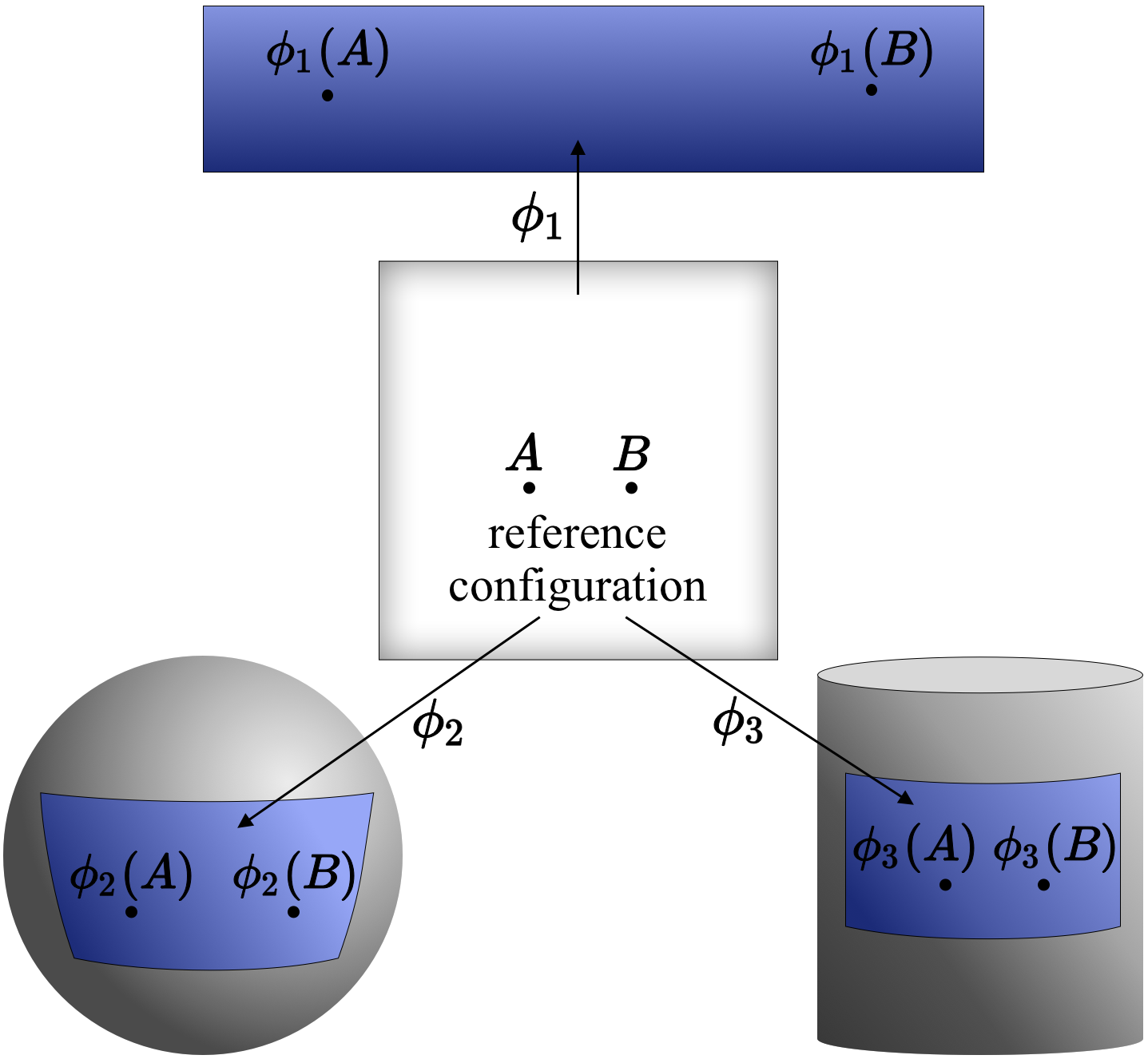
Figure 1: Illustration of the $\phi$ mapping that connects the undeformed elastic body to the deformed one. Under the deformations as described by the mappings $\phi_{i}$ ($i=1,2,3$), the original 2D elastic body of square shape is deformed to a rectangle (by $\phi_{1}$ mapping), to the patches on the sphere (by $\phi_{2}$ mapping) and on the cylinder (by $\phi_{3}$ mapping), respectively.

From the geometric perspective, the deformation is characterized by the variation of the metric from $g_{ab}$ to $\phi^{*}\tilde{g}_{ab}$, both of which are defined on the same manifold $\mathcal{B}$. Specifically, the information of the strain in the deformation is encoded in the difference between $\phi^{*}\tilde{g}_{ab}$ and $g_{ab}$. To illustrate this point, let us consider a curve $\gamma(t)\in(\mathcal{B},g_{ab})$, where $t\in[0,1]$. The length of the line element on $\gamma$ is measured by $g_{ab}$. After the deformation, the curve is mapped to $\phi(\gamma(t))\in(\mathcal{B},\tilde{g}_{ab})$. The length of a line element on $\phi(\gamma)$ measured by $\tilde{g}_{ab}$ is equal to the length of the corresponding line element on $\gamma$ measured by $\phi^{*}\tilde{g}_{ab}$. Therefore, the change of the curve length could be measured by $\phi^{*}\tilde{g}_{ab}-g_{ab}$. As such, it is natural to define the strain tensor on $\mathcal{B}$ as [27, 28]

$$u_{ab}=\bar{g}_{ab}-g_{ab},$$ (1)

where $\bar{g}_{ab}\equiv\phi^{*}\tilde{g}_{ab}$ for simplicity. Note that the definition of strain in Eq.(1) is also applicable to large deformation.

In the following discussion, the Riemannian manifold $(\mathcal{B},\bar{g}_{ab})$ is denoted as $\Sigma$, representing the deformed configuration of the elastic body. The elastic body is initially free of stress, and is thus isometrically embedded in the $(d+1)$-dimensional Euclidean space $\mathcal{E}$. The metric $\bar{g}_{ab}$ on the manifold $\Sigma$ is induced from the metric $\delta_{ab}$ on $\mathcal{E}$ [24, 29, 30], i.e., $\bar{g}_{ab}=\delta_{ab}-N_{a}N_{b}$, where $N_{a}$ is the unit normal covector on $\Sigma$ in $\mathcal{E}$. For example, consider a 2D surface isometrically embedded in $\mathcal{E}$. One may construct the Cartesian coordinates $\{X^{1},X^{2},X^{3}\}$ centered at any point $P$ on the surface; $X^{3}$-axis is perpendicular to the tangent plane at point $P$. The first fundamental form (or the line element) is given explicitly by the metric: $\bar{g}_{\alpha\beta}(\differential X^{\alpha})_{a}(\differential X^{\beta})_{b}=\bar{g}_{\mu\nu}(\differential s^{\mu})_{a}(\differential s^{\nu})_{b}+(\differential X^{3})_{a}(\differential X^{3})_{b}-(\differential X^{3})_{a}(\differential X^{3})_{b}=\bar{g}_{\mu\nu}(\differential s^{\mu})_{a}(\differential s^{\nu})_{b}$, where $\{s^{1},s^{2}\}$ are local coordinates near the point $P$. For spherical surface, $s^{1}=\theta$ and $s^{2}=\phi$, where the polar angle $\theta\in[0,\pi]$ and the azimuthal angle $\phi\in[0,2\pi)$. Note that due to the isometric embedding of $\Sigma$ in $\mathcal{E}$, all of the tensors in this work are regarded as being defined on the tangent space of $\mathcal{E}$, and the lowering (raising) of the indices of a tensor is uniformly implemented by $\delta_{ab}$ ($\delta^{ab}$).

To characterize the displacement field associated with the deformation, we first establish the Cartesian coordinates system of $\mathcal{E}$ by $\{X^{1},\dots,X^{d+1}\}$. The manifolds $(\mathcal{B},g_{ab})$ and $\Sigma$ are thus represented by the $\mathbb{R}^{d+1}$ -valued functions $X_{0}^{\mu}(p)$ and $X^{\mu}(\phi(p))$ ($\forall p\in\mathcal{B}$), respectively. $\bar{X}^{\mu}(p)\equiv X^{\mu}(\phi(p))$. The displacement field on $\mathcal{B}$ is

$$U^{a}=U^{\mu}\quantity(\partialderivative{X^{\mu}})^{a},$$ (2)

where the $\mu$-component of the displacement field $U^{\mu}(p)=\bar{X}^{\mu}(p)-X_{0}^{\mu}(p),\forall p\in\mathcal{B}.$

Construct Hamiltonian of the elastic body The displacement fields $U^{a}$ constitute an infinite dimensional manifold called the configuration space. The Hamiltonian of the elastic body is a scalar on the cotangent bundle of the configuration space, and it can be written formally as [30]:

$$H=T+W=\int_{\Sigma}\rho\quantity(\mathscr{T}+\mathscr{W})\bm{\varepsilon},$$ (3)

where $\mathscr{T}$ and $\mathscr{W}$ are the kinetic energy and elastic potential per unit mass, respectively. $\bm{\varepsilon}$ is the Riemannian volume form compatible with $\bar{g}_{ab}$. $\rho$ is the mass density of the deformed configuration. In this work, $\mathscr{W}$ is a quadratic local function of $u_{ab}$. The gradient of $\mathscr{W}$ is recognized as the Kirchhoff stress tensor:

$$\tau^{ab}=\partialderivative{\mathscr{W}}{u_{ab}}.$$ (4)

$\tau^{ab}$ is a symmetric tensor field on $\mathcal{B}$. In Eq. (3), $\mathscr{T}$ could be written as a quadratic function of the generalized momentum density field $P_{a}$ that is conjugated to $U^{a}$:

$$\mathscr{T}=\frac{1}{2}\mathcal{M}^{ab}P_{a}P_{b}.$$ (5)

It is important to point out that here we introduce the effective mass tensor $\mathcal{M}^{ab}$. $\mathcal{M}^{ab}$ is anisotropic and symmetric, and it is invariant in the deformation of the elastic body. Physically, the anisotropy of $\mathcal{M}^{ab}$ may originate from external potential; for example, the inertial of an electron moving in a crystal is varied along different directions, which is known as the anisotropic Kepler problem [31, 32]. The idea of introducing the anisotropy in the construction of the kinetic energy is inspired by the work on Hamiltonian curl forces [20, 21, 22]. Specifically, it has been proved that a class of non-conservative (i.e., whose curl is not zero) position depending forces can be generated by the element of anisotropy in the kinetic energy term in Hamiltonian. Eq.(3) admits a non-conservative force density, which is crucial for understanding odd elasticity.

Odd elasticity in Hamilton’s Equations The Hamilton equations based on Eq.(3) are [33]

$$\partialderivative{U^{a}}{t} =\functionalderivative{H}{P_{a}}=\rho\sqrt{\bar{g}}\mathcal{M}^{ab}P_{b},$$ (6a)

$$\partialderivative{P_{a}}{t} =-\functionalderivative{H}{U^{a}}=2\sqrt{\bar{g}}f_{a},$$ (6b)

where $f_{a}=\bar{g}_{b}{}^{c}\partial_{c}\quantity(\bar{g}_{ad}\sigma^{db})$. $\bar{g}$ is the determinant of $\bar{g}_{ab}$; the Cauchy stress tensor $\sigma^{ab}=\rho\tau^{ab}$ [30]; $\partial_{c}$ is the Cartesian derivative operator on $\mathcal{E}$ acting on the embedding coordinates $\{\bar{X}^{\mu}\}$ of $\Sigma$.

By combining Eq. (6a) and Eq. (6b), we obtain the dynamic equation of the manifold $\Sigma$ as

$$\partialderivative{V^{a}}{t}=M^{ab}f_{b}\equiv F^{a},$$ (7)

where the displacement velocity field $V^{a}\equiv\partialderivative*{U^{a}}{t}$ and the symmetric tensor field $M^{ab}\equiv 2\rho\bar{g}\mathcal{M}^{ab}$. According to Eq. (7), $F^{a}$ is recognized as the Newtonian force per unit mass.

Without any loss of generality, $M^{ab}$ is decomposed as

$$M^{ab}=M\delta^{ab}+\Omega^{ab},$$ (8)

where $M=\delta_{ab}M^{ab}/(d+1)$, and $\Omega^{ab}$ is a traceless symmetric tensor field. Here, we shall emphasize that the anisotropic effect in the kinetic energy is captured by $\Omega^{ab}$. By Eq.(8), we cast $F^{a}$ in the following form

$$F^{a}=Mf^{a}+\Omega^{ab}f_{b}.$$ (9)

Now, let us focus on Eq.(9). First of all, it can be shown that the first term in Eq.(9) is conservative by letting $M=1/\rho$:

$$Mf_{a} =-\frac{1}{2\rho\sqrt{\bar{g}}}\functionalderivative{H}{U^{a}}=-\frac{1}{2}\quantity(\differential\mathcal{W})_{a},$$ (10)

where $(\differential)_{a}$ is the exterior derivative operator on $\mathcal{E}$. Since $\differential(Mf)_{ab}=0$, we conclude that $f_{a}$ is conservative. $f^{a}$ is essentially the force per unit volume generated from the elastic potential [28, 34, 35, 36].

We proceed to examine the second term in Eq. (9). Substituting the expression of $f_{a}$ in Eq. (9) leads to the Newtonian force per unit volume as

$$\rho F^{a} =\bar{g}_{b}{}^{c}\partial_{c}\sigma^{ab}+\rho\Omega^{ad}\bar{g}_{b}{}^{c}\partial_{c}\quantity(\bar{g}_{de}\sigma^{eb})$$

$$=\bar{g}_{b}{}^{c}\partial_{c}\quantity(\sigma^{ab}+\hat{\sigma}^{ab})-\bar{g}_{bd}\sigma^{dc}\partial_{c}\quantity(\rho\Omega^{ab}),$$ (11)

where $\hat{\sigma}^{ab}\equiv\rho\Omega^{ac}\bar{g}_{cd}\sigma^{db}$. Note that $\hat{\sigma}^{ab}$ is not symmetric. Furthermore, $\hat{\sigma}^{ab}$ does not live in the tangent space of $\Sigma$ because of the acting of $\Omega^{ac}\bar{g}_{cd}$. For spatially-slowly-varying external potential, the gradient of $\rho\Omega^{ab}$ that is coupled to external potential could be regarded as a small quantity. Therefore, the last term in Eq. (11) is much smaller than the second term; note that $\bar{g}_{b}{}^{c}\partial_{c}\hat{\sigma}^{ab}=\bar{g}_{b}{}^{c}\partial_{c}(\rho\Omega^{ad}\bar{g}_{de}\sigma^{eb})$. As such, the last term could be neglected. The anisotropic effect boils down to the modification of $\hat{\sigma}^{ab}$ in $\sigma^{ab}$ as shown in the first bracket in Eq. (11).

To reveal the non-conservative nature of the second term in Eq. (9), we analyze the work done by the total stress per unit mass in a cyclic deformation. In the deformation process, the instantaneous strain state of the elastic body is denoted by $u_{ab}(t)$, which is represented by a point in the space of the strain field $u_{ab}$. The cycle of deformation is thus described by a loop $\eta(t)$ in the strain space. $t\in[0,T]$. $\eta(0)=\eta(T)$. The work done per unit mass in a cycle of deformation is [8, 7]:

$$\Delta\mathscr{A} =\oint_{\eta(t)}\quantity(\tau^{ab}+\hat{\tau}^{ab})\differential u_{ab}$$

$$=\frac{1}{2}\int_{S}\quantity(\partialderivative{\tau^{ab}}{u_{cd}}+\partialderivative{\hat{\tau}^{ab}}{u_{cd}})\differential u_{ab}\wedge\differential u_{cd},$$

$$\equiv\frac{1}{2}\int_{S}T^{abcd}\differential u_{ab}\wedge\differential u_{cd},$$ (12)

where $\hat{\tau}^{ab}=\hat{\sigma}^{ab}/\rho$, and $S$ is the surface enclosed by $\eta(t)$. Stokes’s theorem is used in the derivation for Eq. (12). Since the exterior product is antisymmetric, the stress is conservative (such that $\Delta\mathscr{A}=0$ in the cyclic deformation) if and only if $T^{abcd}$ possesses the major index symmetry, i.e., $T^{abcd}=T^{cdab}$. Especially, quasi-static cyclic deformation can be realized by applying suitable external force on $\Sigma$. $\Delta\mathscr{A}$ is then equal to the work done by the external force.

We analyze the first term of $T^{abcd}$ in Eq. (12). From the expression for $\mathscr{W}$

$$\mathscr{W}=C^{abcd}u_{ab}u_{cd},$$ (13)

where $C^{abcd}$ is the elastic modulus tensor with major index symmetry (i.e, $C^{abcd}=C^{cdab}$), we obtain the linear constitutive relation

$$\tau^{ab}=C^{abcd}u_{cd}.$$ (14)

Due to the major index symmetry of $C^{abcd}$, the first term of $T^{abcd}$ satisfies $\partialderivative*{\tau^{ab}}{u_{cd}}=\partialderivative*{\tau^{cd}}{u_{ab}}$, which indicates the conservative nature of $\tau^{ab}$. In other words, the work done by $\tau^{ab}$ is zero in a cyclic deformation.

For the second term in $T^{abcd}$, from the definition of $\hat{\sigma}^{ab}$ and Eq. (14), we have

$$\hat{\tau}^{ab} =\rho\Omega^{ac}\bar{g}_{cd}\tau^{db}$$

$$=\rho\Omega^{ae}\quantity(g_{ef}+u_{ef})C^{fbcd}u_{cd}$$

$$=\hat{C}^{abcd}u_{cd}+\hat{D}^{abcdef}u_{cd}u_{ef},$$ (15)

where

$$\hat{C}^{abcd}=\rho\Omega^{ae}g_{ef}C^{fbcd},\quad\hat{D}^{abcdef}=\rho\Omega^{ac}C^{dbef}.$$ (16)

In the nonlinear constitutive relation in Eq. (15), the quadratic term naturally arises in the expansion of $\bar{g}_{cd}$ as the sum of the metric $g_{cd}$ of the reference configuration and the strain field $u_{cd}$. Furthermore, the anisotropic tensor $\Omega^{ab}$ leads to the anisotropic nature of the elastic moduli $\hat{C}^{abcd}$ and $\hat{D}^{abcdef}$. By Eq. (15), the second term of $T^{abcd}$ is obtained

$$\partialderivative{\hat{\tau}^{ab}}{u_{cd}}=\hat{C}^{abcd}+\quantity(\hat{D}^{abcdef}+\hat{D}^{abef(cd)})u_{ef}$$ (17)

Here, it is important to point out that in Eq. (16), the involvement of the $\Omega^{ab}$-tensor breaks the major index symmetry of $\hat{C}^{abcd}$, as well as that of the second and the third terms in the right hand side of Eq. (17). Consequently, $\hat{\tau}^{ab}$ is non-conservative according to Eq. (17).

Note that both $\hat{C}^{abcd}$ and $\hat{D}^{abcdef}$ in Eq. (16) are invariant in the deformation of $\Sigma$. The reason is as follows. In the expressions for $\hat{C}^{abcd}$ and $\hat{D}^{abcdef}$, both the elastic modulus tensor $C^{abcd}$ and the metric $g_{ab}$ are independent of the deformation of $\Sigma$. Regarding the factor $\rho\Omega^{ab}$, according to Eq. (8) and the definition for $M^{ab}$, $\rho\Omega^{ab}=2\rho^{2}\bar{g}\mathcal{M}^{ab}-\delta^{ab}=2\rho_{0}^{2}g\mathcal{M}^{ab}-\delta^{ab}$, where $\rho_{0}$ is the mass density of the reference configuration. $\rho\Omega^{ab}$ is therefore invariant in the deformation of $\Sigma$.

In the regime of small deformation, where the quadratic term in Eq. (15) can be neglected, the constitutive relation of $\hat{\tau}^{ab}$ becomes linear:

$$\hat{\tau}^{ab}=\hat{C}^{abcd}u_{cd}.$$ (18)

The broken major index symmetry of $\hat{C}^{abcd}$ indicates the presence of the antisymmetric (odd) part in the elastic modulus tensor, which is responsible for the non-conservativity of the stress and the extra work occurring in cyclic deformations. As such, $\hat{C}^{abcd}$ is called the odd elastic modulus in literature [8]. Microscopic mechanism for odd elasticity has been attributed to various non-conservative interparticle forces. Here, the odd elasticity as characterized by the $\hat{C}^{abcd}$-tensor in Eq. (18) is derived from the anisotropic effective mass in the Hamiltonian formalism.

Example of 2D planar deformation In this section, we illustrate the emergence of odd elasticity for the simple case of planar deformation of a 2D elastic body under small deformation approximation.

The strain tensor $u_{ab}$ in the deformation can be expanded as $u_{ab}=u_{\mu}\mathfrak{e}^{\mu}{}_{ab}$, where $\mathfrak{e}^{\mu}{}_{ab}$ is a set of orthonormal tensor bases on the reference configuration equipped with a local orthonormal frame fields $\{e_{1}{}^{a},e_{2}{}^{a}\}$ [8]:

$$\mathfrak{e}^{1}{}_{ab}=e^{1}{}_{a}e^{1}{}_{b}+e^{2}{}_{a}e^{2}{}_{b},$$ (19a)

$$\mathfrak{e}^{2}{}_{ab}=e^{2}{}_{a}e^{1}{}_{b}-e^{1}{}_{a}e^{2}{}_{b},$$ (19b)

$$\mathfrak{e}^{3}{}_{ab}=e^{1}{}_{a}e^{1}{}_{b}-e^{2}{}_{a}e^{2}{}_{b},$$ (19c)

$$\mathfrak{e}^{4}{}_{ab}=e^{1}{}_{a}e^{2}{}_{b}+e^{2}{}_{a}e^{1}{}_{b}.$$ (19d)

$u_{\mu}$ characterizes the following local modes of deformation: dilation, rotation, and shearing. The stress tensor can also be expanded as $\tau^{ab}=\tau^{\mu}\mathfrak{e}_{\mu}{}^{ab}$, where $\tau^{\mu}$ are associated with pressure, torque density and shear stress.

The rotationally symmetric elastic modulus tensor field $C^{abcd}$ could be written as [33]:

$$C^{abcd}=\lambda g^{ab}g^{cd}+2\mu g^{a(c}g^{d)b},$$ (20)

where $\lambda$ and $\mu$ are Lamé coefficients. In the tensor bases of $\{\mathfrak{e}^{\mu}{}_{ab}\}$, $g_{ab}=\mathfrak{e}^{1}{}_{ab}$, and $C^{abcd}=C^{\mu\nu}\mathfrak{e}_{\mu}{}^{ab}\mathfrak{e}_{\nu}{}^{cd}$. From Eq. (20), we obtain

$$C^{\mu\nu}=\matrixquantity(\lambda+\mu&0&0&0\\ 0&0&0&0\\ 0&0&\mu&0\\ 0&0&0&\mu).$$ (21)

Correspondingly, Eq. (14) is expressed as $\tau^{\mu}=C^{\mu\nu}u_{\nu}$. $\lambda+\mu$ and $\mu$ characterize the isotropic stretching rigidity and the isotropic shear rigidity, respectively. Note that the matrix in Eq. 21 is invariant under the rotation of $\{e_{1}{}^{a},e_{2}{}^{a}\}$.

We proceed to discuss the components $\hat{C}^{\mu\nu}$. By expanding the traceless tensor $\rho\Omega^{ab}$ in the tensor bases of $\{e_{1}{}^{a},e_{2}{}^{a}\}$ as

$$\rho\Omega^{ab}= \kappa e_{1}{}^{a}e_{1}{}^{b}+\zeta e_{1}{}^{a}e_{2}{}^{b}+\zeta e_{2}{}^{a}e_{1}{}^{b}-\kappa e_{2}{}^{a}e_{2}{}^{b},$$ (22)

where $\kappa$ and $\zeta$ are scalars, we finally have Since $\hat{C}^{abcd}=\hat{C}^{\mu\nu}\mathfrak{e}_{\mu}{}^{ab}\mathfrak{e}_{\nu}{}^{cd}$, the abstract index exchange $ab\leftrightarrow cd$ in $\hat{C}^{abcd}$ is identical to the label exchange $\mu\leftrightarrow\nu$ in $\hat{C}^{\mu\nu}$. Eq. (LABEL:coordinates_hC) shows that $\hat{C}^{\mu\nu}\neq\hat{C}^{\nu\mu}$, and therefore $\hat{C}^{abcd}\neq\hat{C}^{cdab}$. This key feature of the broken major symmetry is exactly the mathematical structure underlying the phenomenon of odd elasticity. The upper right $2\times 2$ submatrix in Eq. (LABEL:coordinates_hC) connects shear strain with pressure and torque, and the lower left $2\times 2$ submatrix connects dilation with shear stress. The existence of these two non-zero submatrices is an indicator for the anisotropy of $\hat{C}^{abcd}$ [8].

In summary, from the perspective of geometry, we model a $d$-dimensional continuum elastic body as a Riemannian manifold embedded in the $(d+1)$-dimensional Euclidean space, and construct a Hamiltonian framework for the elastic body of finite strain. It is shown that the antisymmetry of the elastic modulus tensor is originated from the anisotropic mass tensor in the kinetic term. We also derive the non-conservative stress and the associated nonlinear constitutive relation, where the nonlinearity is caused by the intrinsic geometry of the deformed elastic body. The Hamiltonian formalism constructed in this work for characterizing odd elasticity also allows one to explore the physics of odd elasticity in dynamical regime.

Acknowledgements This work was supported by the National Natural Science Foundation of China (Grants No. BC4190050).

Supplemental Material

In the following, we present more information about the derivation of the induced metric and strain, the variational derivatives of the Hamiltonian, and the isometric symmetry of elastic modulus tensor.

Appendix A Expressions for the induced metric and strain

In this section, we derive the expressions for the induced metric and strain. Note that we employ the abstract index notation in Roman letters to represent a tensor; the tensor components are labeled by Greek letters.

First of all, for any local coordinates system $\{s^{1},\dots,s^{d}\}$ on $\mathcal{B}$, the associated coordinates base vector on its embedding

$$\quantity(\partialderivative{s^{\mu}})^{a}=\partialderivative{\bar{X}^{\nu}}{s^{\mu}}\quantity(\partialderivative{\bar{X}^{\nu}})^{a},$$ (23)

where $\bar{X}^{\nu}$ is the Cartesian coordinates of the embedding of deformed configuration $\Sigma$ in the Euclidean space $\mathcal{E}$.

The isometric embedding of $\Sigma$ in the Euclidean space $\mathcal{E}$ indicates that

$$\bar{g}_{ab}=\delta_{ab}-N_{a}N_{b},$$ (24)

where $N_{a}$ is the unit normal covector on $\Sigma$. Therefore,

$$\bar{g}_{\mu\nu} =\bar{g}_{ab}\quantity(\partialderivative{s^{\mu}})^{a}\quantity(\partialderivative{s^{\nu}})^{b}$$

$$=\quantity(\delta_{ab}-N_{a}N_{b})\quantity(\partialderivative{s^{\mu}})^{a}\quantity(\partialderivative{s^{\nu}})^{b}$$

$$=\delta_{ab}\quantity(\partialderivative{s^{\mu}})^{a}\quantity(\partialderivative{s^{\nu}})^{b}$$

$$=\delta_{\tau\rho}\partialderivative{\bar{X}^{\tau}}{s^{\mu}}\partialderivative{\bar{X}^{\rho}}{s^{\nu}}$$

$$=\partialderivative{\bar{X}_{\rho}}{s^{\mu}}\partialderivative{\bar{X}^{\rho}}{s^{\nu}}.$$ (25)

Here $\delta_{ab}$ is the Euclid metric of $\mathcal{E}$, and $\delta_{\tau\rho}$ is Kronecker delta which is the components of $\delta_{ab}$ in Cartesian coordinates. In the derivation of Eq. (25), we use the fact that $\quantity(\partialderivative*{s^{\mu}})^{a}N_{a}=0$. One has the similar result for $g_{\mu\nu}$ as

$$g_{\mu\nu}=\partialderivative{X_{0\rho}}{s^{\mu}}\partialderivative{X_{0}^{\rho}}{s^{\nu}},$$ (26)

where $X_{0}^{\rho}$ is the Cartesian coordinates of the embedding of reference configuration.

By substituting Eqs. (25) and (26) into the following expression of $u_{ab}$

$$u_{ab}=\bar{g}_{ab}-g_{ab},$$ (27)

we obtain

$$u_{ab} =\quantity(\partialderivative{\bar{X}_{\rho}}{s^{\mu}}\partialderivative{\bar{X}^{\rho}}{s^{\nu}}-\partialderivative{X_{0\rho}}{s^{\mu}}\partialderivative{X_{0}^{\rho}}{s^{\nu}})\quantity(\differential s^{\mu})_{a}\quantity(\differential s^{\nu})_{b}$$

$$=\nabla_{a}\bar{X}_{\rho}\nabla_{b}\bar{X}^{\rho}-\nabla_{a}X_{0\rho}\nabla_{b}X_{0}^{\rho},$$ (28)

where $\nabla_{b}$ is the covariant derivative operator on $\Sigma$. $\nabla_{b}$ is metric compatible, i.e., $\nabla_{b}\bar{g}_{ac}=0$. Equation (28) shows that $u_{ab}$ could be regarded as a local function of $\nabla_{a}\bar{X}^{\rho}$.

Appendix B Variational derivatives of the Hamiltonian

In this section, we present the variational derivatives of the Hamiltonian defined on the manifold $\mathcal{B}$, which is recorded here

$$H=T+W=\frac{1}{2}\int\differential[d]{s}\rho_{0}\sqrt{g}\mathcal{M}^{ab}P_{a}P_{b}+\int\differential[d]{s}\rho_{0}\sqrt{g}\mathscr{W}.$$ (29)

The variational derivative of the Hamiltonian with respect to the generalized momentum density field $P_{a}$ is

$$\functionalderivative{H}{P_{a}}=\functionalderivative{T}{P_{a}}=\rho_{0}\sqrt{g}\mathcal{M}^{ab}P_{b}.$$ (30)

To obtain the variational derivative of the Hamiltonian with respect to $U^{a}$, we first calculate

$$\delta W= \int\differential[d]{s}\rho_{0}\sqrt{g}\delta\mathscr{W}$$

$$= \int\differential[d]{s}\rho\sqrt{\bar{g}}\partialderivative{\mathscr{W}}{u_{ab}}\delta u_{ab}$$

$$= 2\int\differential[d]{s}\sqrt{\bar{g}}\sigma^{ab}\nabla_{a}\bar{X}_{\rho}\nabla_{b}\delta\bar{X}^{\rho}$$

$$= 2\int\differential[d]{s}\sqrt{\bar{g}}\nabla_{b}\quantity(\sigma^{ab}\nabla_{a}\bar{X}_{\rho}\delta\bar{X}^{\rho})-2\int\differential[d]{s}\sqrt{\bar{g}}\nabla_{b}\quantity(\sigma^{ab}\nabla_{a}\bar{X}_{\rho})\delta\bar{X}^{\rho}$$

$$= -2\int\differential[d]{s}\sqrt{\bar{g}}\nabla_{b}\quantity(\sigma^{ab}\nabla_{a}\bar{X}_{\rho})\delta\bar{X}^{\rho}\ ,$$ (31)

where the Cauchy stress tensor $\sigma^{ab}\equiv\rho\tau^{ab}$. Note that from the first line to the second line in Eq. (31), the domain of integration is changed from the reference configuration to $\Sigma$. In the last equality, we drop the divergence term to the boundary term by utilizing Gauss’s theorem; only the energy variation in the interior of the body is considered.

Now, we calculate the variational derivative of the Hamiltonian with respect to the displacement field $U^{a}$:

$$\functionalderivative{H}{U^{a}} =\functionalderivative{W}{U^{a}}$$

$$=\functionalderivative{W}{\bar{X}^{\mu}}\quantity(\differential\bar{X}^{\mu})_{a}$$

$$=-2\sqrt{\bar{g}}\quantity(\differential\bar{X}^{\mu})_{a}\nabla_{c}\quantity(\sigma^{bc}\nabla_{b}\bar{X}_{\mu})$$

$$=-2\sqrt{\bar{g}}\quantity(\differential\bar{X}^{\mu})_{a}\bar{g}_{c}{}^{d}\partial_{d}\quantity[\sigma^{bc}\bar{g}_{b}{}^{e}\quantity(\differential\bar{X}_{\mu})_{e}]$$

$$=-2\sqrt{\bar{g}}\bar{g}_{c}{}^{d}\partial_{d}\quantity[\sigma^{bc}\bar{g}_{b}{}^{e}\quantity(\differential\bar{X}^{\mu})_{a}\quantity(\differential\bar{X}_{\mu})_{e}]$$

$$=-2\sqrt{\bar{g}}\bar{g}_{c}{}^{d}\partial_{d}\quantity(\sigma^{bc}\bar{g}_{b}{}^{e}\delta_{ae})$$

$$=-2\sqrt{\bar{g}}\bar{g}_{c}{}^{d}\partial_{d}\quantity(\bar{g}_{ab}\sigma^{bc})$$

$$\equiv-2\sqrt{\bar{g}}f_{a}.$$ (32)

$\partial_{a}$ is the derivative operator in the Cartesian coordinates on $\mathcal{E}$; $\partial_{a}\quantity(\differential\bar{X}_{\mu})_{b}=0$. $(\differential)_{a}$ is the exterior derivative operator on $\mathcal{E}$. $\bar{g}_{a}{}^{b}$ is a projection operator: $\bar{g}_{a}{}^{b}=\bar{g}_{ac}\delta^{cb}=\delta_{a}{}^{b}-N_{a}N^{b}$.

Here, it is of interest to point out that in general $f_{a}$ is not tangent to $\Sigma$, which is shown below

$$f_{a} =\bar{g}_{c}{}^{d}\partial_{d}\quantity(\bar{g}_{ab}\sigma^{bc})$$

$$=\bar{g}_{c}{}^{d}\partial_{d}\quantity(\sigma^{bc}\bar{g}_{b}{}^{e}\delta_{ae})$$

$$=\delta_{ae}\bar{g}_{c}{}^{d}\partial_{d}\quantity(\sigma^{bc}\bar{g}_{b}{}^{e})$$

$$=\delta_{ae}\quantity(\bar{g}_{b}{}^{e}\bar{g}_{c}{}^{d}\partial_{d}\sigma^{bc}+\sigma^{bc}\bar{g}_{c}{}^{d}\partial_{d}\bar{g}_{b}{}^{e})$$

$$=\delta_{ae}\quantity(\nabla_{c}\sigma^{ec}-\sigma^{bd}N^{e}\partial_{d}N_{b})$$

$$=\bar{g}_{ab}\nabla_{c}\sigma^{bc}-N_{a}\sigma^{bc}K_{bc},$$ (33)

where $K_{bc}$ is the extrinsic curvature of $\Sigma$. In the derivation, we use the definition of extrinsic curvature $K_{bc}=\bar{g}_{b}{}^{d}\bar{g}_{c}{}^{e}\partial_{d}N_{e}$ and the fact that $\sigma^{ab}N_{b}=0$. The first and second terms in Eq. (33) are the tangent and normal components of $f_{a}$ [34, 35, 36]. For example, in the case of $\phi_{2}$ in Fig. 1 of the main text, the normal force supporting $\Sigma$ on the sphere is $(e_{r})^{a}\sigma^{b}{}_{b}/R$, where $R$ is the radius of the sphere and $(e_{r})^{a}$ is the unit normal vector perpendicular to the spherical surface.

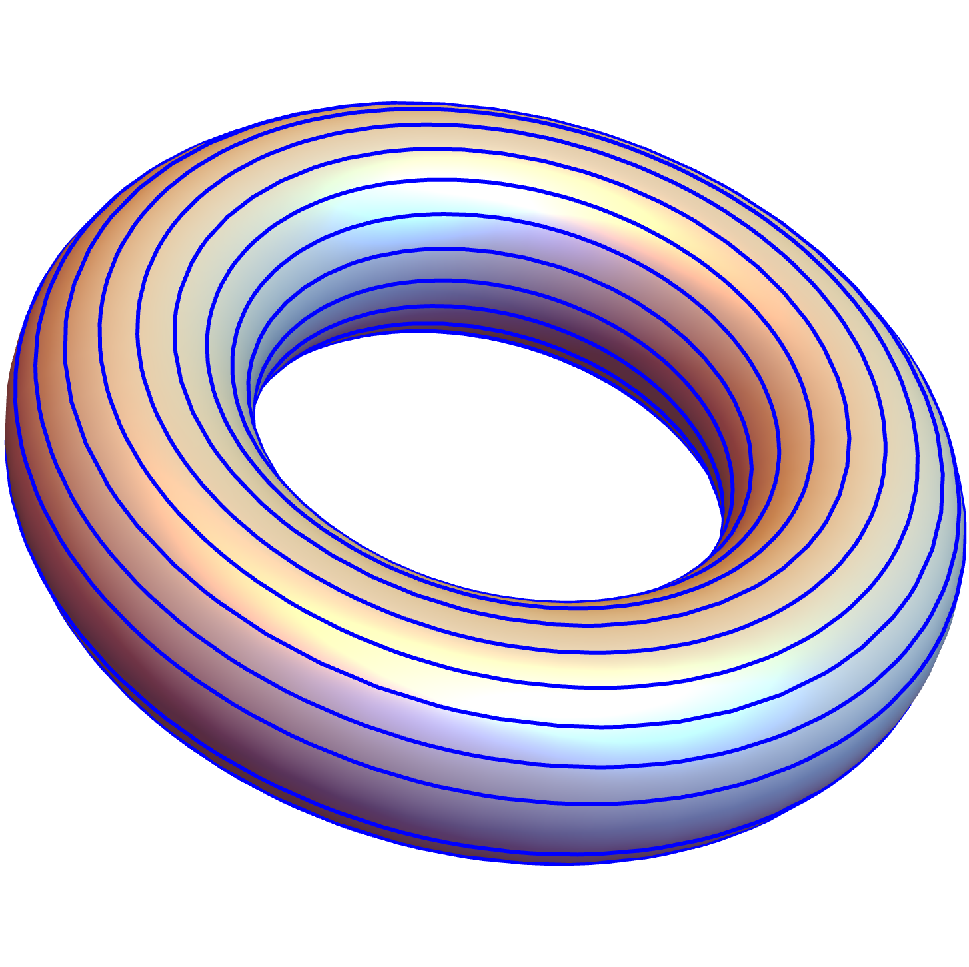
(a) Torus

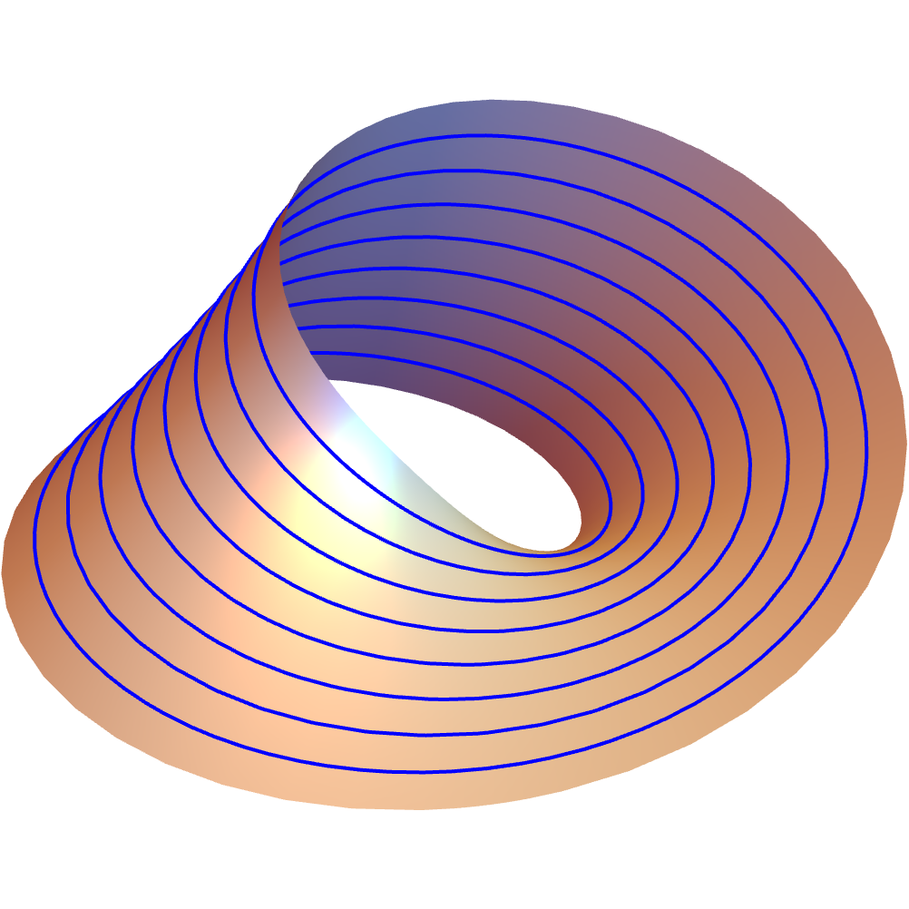
(b) Möbius strip

Figure 2: Illustrations of 2D torus and Möbius strip. The tangent vectors of the lines constitute the Killing vector fields on these two surfaces.

Appendix C The isometric symmetry of elastic modulus tensor

In the main text, we present the following expression for the rotationally symmetric elastic modulus tensor in an axisymmetric continuum elastic body:

$$C^{abcd}=\lambda g^{ab}g^{cd}+2\mu g^{a(c}g^{d)b},$$ (34)

where $\lambda$ and $\mu$ are Lamé coefficients. In this section, we present the derivation for Eq. (34).

Consider an axisymmetric continuum elastic body. Its rotation as a whole belongs to a special isometric mapping that could be generated by a Killing vector field $v^{a}$. By the definition of the Killing vector field, the displacement of the points from $s^{\mu}$ to $s^{\mu}+v^{\mu}\epsilon$ leaves the distance relationships unchanged. In other words, the displacement of $v^{\mu}\epsilon$ defines an isometric mapping. In Fig. 2(a), we present a 2D torus as an example of the axisymmetric elastic body. The tangent vectors of the toroidal lines constitute the Killing vector field on the torus. The elastic modulus tensor as associated with infinitesimal volume element possesses the rotational symmetry in the sense that it is invariant along the toroidal lines.

The rotational symmetry of the elastic modulus tensor $C^{abcd}$ is expressed by the zero Lie derivative of $C^{abcd}$ along the direction as specified by the Killing vector on the reference configuration [37]:

$$\mathscr{L}_{v}C^{abcd}\equiv v^{e}\nabla_{e}C^{abcd}-C^{ebcd}\nabla_{e}v^{a}-C^{aecd}\nabla_{e}v^{b}-C^{abed}\nabla_{e}v^{c}-C^{abce}\nabla_{e}v^{d}=0,$$ (35)

where $v^{a}$ is a Killing vector field satisfying $\nabla_{(a}v_{b)}=0$, and $\nabla_{a}$ is the covariant derivative operator on the reference configuration. $C^{abcd}$ as constructed by the tensor product of $g^{ab}$-tensors satisfies Eq. (35); note that $\mathscr{L}_{v}g^{ab}=0$. Specifically, there are three kinds of index permutations of the tensor product:

$$C^{abcd}=\lambda g^{ab}g^{cd}+\mu_{1}g^{ac}g^{bd}+\mu_{2}g^{ad}g^{bc},$$ (36)

where $\lambda$, $\mu_{1}$ and $\mu_{2}$ are constant scalars on $\mathcal{B}$.

Due to the extra requirements for the conservation of angular momentum and the conservative nature of stress [8],

$$C^{abcd}=C^{cdab}=C^{bacd}\ .$$ (37)

The first equality is automatically satisfied for Eq. (36). The second equality is satisfied if $\mu_{1}=\mu_{2}=\mu$. The final expression for $C^{abcd}$ that satisfies both Eqs. (36) and (37) is

$$C^{abcd}=\lambda g^{ab}g^{cd}+2\mu g^{a(c}g^{d)b}.$$ (38)

For Euclidean reference configuration, the components of $C^{abcd}$ in Cartesian coordinates system are

$$C^{\mu\nu\eta\gamma}=\lambda\delta^{\mu\nu}\delta^{\eta\gamma}+2\mu\delta^{\mu(\eta}\delta^{\gamma)\nu}.$$ (39)

By making use of the linear constitutive relation, the elastic potential can be expressed as

$$W=\int\differential[d]{s}\rho_{0}\quantity[\lambda\quantity(u_{\eta\eta})^{2}+2\mu\quantity(u_{\eta\gamma})^{2}],$$ (40)

where $\differential[d]{s}$ is the volume element of Cartesian coordinates on the reference configuration. In comparison with the linear elasticity theory, the parameters $\lambda$ and $\mu$ are recognized as the Lamé coefficients [2].

Note that Eq. (35) could be used to describe the general case that the elastic modulus tensor is invariant along the lines of the Killing vectors, i.e., the isometric symmetry of the elastic modulus tensor. For example, on the Möbius strip in Fig. 2(b), the tangent vectors of the lines constitute the Killing vector field; the isometric mapping of the Möbius strip is generated by this Killing vector field. $C^{abcd}$ that satisfies Eq. (35) is invariant along these lines. This is the generalization of the rotational symmetry of the elastic modulus tensor of axisymmetric continuum elastic body as discussed in this section.

References

- Truesdell [1952] C. A. Truesdell, The mechanical foundations of elasticity and fluid dynamics, Indiana Univ. Math. J. 1, 125 (1952).
- Landau and Lifshitz [1960] L. D. Landau and E. M. Lifshitz, Theory of Elasticity (Pergamon, Oxford, 1960).
- Chen et al. [2021] Y. Chen, X. Li, C. Scheibner, V. Vitelli, and G. Huang, Realization of active metamaterials with odd micropolar elasticity, Nat. Commun. 12, 5935 (2021).
- Brandenbourger et al. [2021] M. Brandenbourger, C. Scheibner, J. Veenstra, V. Vitelli, and C. Coulais, Limit cycles turn active matter into robots, arXiv:2108.08837 (2021).
- Bililign et al. [2022] E. S. Bililign, F. Balboa Usabiaga, Y. A. Ganan, A. Poncet, V. Soni, S. Magkiriadou, M. J. Shelley, D. Bartolo, and W. T. M. Irvine, Motile dislocations knead odd crystals into whorls, Nat. Phys. 18, 212 (2022).
- Salbreux and Jülicher [2017] G. Salbreux and F. Jülicher, Mechanics of active surfaces, Phys. Rev. E 96, 032404 (2017).
- Fossati et al. [2022] M. Fossati, C. Scheibner, M. Fruchart, and V. Vitelli, Odd elasticity and topological waves in active surfaces, arXiv:2210.03669 (2022).
- Scheibner et al. [2020] C. Scheibner, A. Souslov, D. Banerjee, P. Surówka, W. T. M. Irvine, and V. Vitelli, Odd elasticity, Nat. Phys. 16, 475 (2020).
- Fruchart et al. [2023] M. Fruchart, C. Scheibner, and V. Vitelli, Odd viscosity and odd elasticity, Annu. Rev. Condens. Matter Phys. 14, 471 (2023).
- Braverman et al. [2021] L. Braverman, C. Scheibner, B. VanSaders, and V. Vitelli, Topological defects in solids with odd elasticity, Phys. Rev. Lett. 127, 268001 (2021).
- Poncet and Bartolo [2022] A. Poncet and D. Bartolo, When soft crystals defy newton’s third law: Nonreciprocal mechanics and dislocation motility, Phys. Rev. Lett. 128, 048002 (2022).
- Happel and Brenner [1983] J. Happel and H. Brenner, Low Reynolds Number Hydrodynamics: with Special Applications to Particulate Media, Vol. 1 (Springer, 1983).
- Jäger and Klapp [2011] S. Jäger and S. H. L. Klapp, Pattern formation of dipolar colloids in rotating fields: layering and synchronization, Soft Matter 7, 6606 (2011).
- Brun et al. [2012] M. Brun, I. S. Jones, and A. B. Movchan, Vortex-type elastic structured media and dynamic shielding, Proc. R. Soc. A. 468, 3027 (2012).
- Nash et al. [2015] L. M. Nash, D. Kleckner, A. Read, V. Vitelli, A. M. Turner, and W. T. M. Irvine, Topological mechanics of gyroscopic metamaterials, Proc. Natl. Acad. Sci. U.S.A. 112, 14495 (2015).
- Tkachenko [1969] V. K. Tkachenko, Elasticity of Vortex Lattices, Soviet Journal of Experimental and Theoretical Physics 29, 945 (1969).
- Nguyen et al. [2020] D. X. Nguyen, A. Gromov, and S. Moroz, Fracton-elasticity duality of two-dimensional superfluid vortex crystals: defect interactions and quantum melting, SciPost Phys. 9, 076 (2020).
- Ochoa et al. [2017] H. Ochoa, S. K. Kim, O. Tchernyshyov, and Y. Tserkovnyak, Gyrotropic elastic response of skyrmion crystals to current-induced tensions, Phys. Rev. B 96, 020410 (2017).
- Benzoni et al. [2021] C. Benzoni, B. Jeevanesan, and S. Moroz, Rayleigh edge waves in two-dimensional crystals with lorentz forces: From skyrmion crystals to gyroscopic media, Phys. Rev. B 104, 024435 (2021).
- Berry and Shukla [2012] M. V. Berry and P. Shukla, Classical dynamics with curl forces, and motion driven by time-dependent flux, J. Phys. A: Math. 45, 305201 (2012).
- Berry and Shukla [2013] M. V. Berry and P. Shukla, Physical curl forces: dipole dynamics near optical vortices, J. Phys. A: Math. 46, 422001 (2013).
- Berry and Shukla [2015] M. V. Berry and P. Shukla, Hamiltonian curl forces, Proc. R. Soc. A. 471, 20150002 (2015).
- Efrati et al. [2009] E. Efrati, E. Sharon, and R. Kupferman, Elastic theory of unconstrained non-euclidean plates, J. Mech. Phys. Solids 57, 762 (2009).
- Kupferman et al. [2017] R. Kupferman, E. Olami, and R. Segev, Continuum dynamics on manifolds: Application to elasticity of residually-stressed bodies, J. Elast. 128, 61 (2017).
- Noll [1978] W. Noll, A general framework for problems in the statics of finite elasticity, in Contemporary Developments in Continuum Mechanics and Partial Differential Equations, North-Holland Mathematics Studies, Vol. 30, edited by G. M. de la Penha and L. A. J. Medeiros (North-Holland, 1978) pp. 363–387.
- Rougée [1992] P. Rougée, The intrinsic lagrangian metric and stress variables, in Finite Inelastic Deformations — Theory and Applications, edited by D. Besdo and E. Stein (Springer, Berlin, Heidelberg, 1992) pp. 217–226.
- Bilby et al. [1955] B. A. Bilby, R. Bullough, E. Smith, and J. M. Whittaker, Continuous distributions of dislocations: a new application of the methods of non-riemannian geometry, Proc. R. Soc. Lond. A 231, 263 (1955).
- Kochetov and Osipov [1999] E. A. Kochetov and V. A. Osipov, Gauge theory of disclinations on fluctuating elastic surfaces, J. Phys. A: Math. Gen. 32, 1961 (1999).
- Segev and Epstein [2020] R. Segev and M. Epstein, eds., Geometric Continuum Mechanics, Adv. Mech. Math., Vol. 43 (Cham: Birkhäuser, 2020).
- Kolev and Desmorat [2021] B. Kolev and R. Desmorat, An intrinsic geometric formulation of hyper-elasticity, pressure potential and non-holonomic constraints, J. Elast. 146, 29 (2021).
- Gutzwiller [1973] M. C. Gutzwiller, The anisotropic kepler problem in two dimensions, J. Math. Phys. 14, 139 (1973).
- Gutzwiller [2013] M. C. Gutzwiller, Chaos in Classical and Quantum Mechanics (Springer, New York, 2013).
- [33] See Supplemental Material for more information about the derivation of the induced metric and strain, the variational derivatives of the Hamiltonian, and isometric symmetry of elastic modulus tensor.
- Capovilla and Guven [2002] R. Capovilla and J. Guven, Stresses in lipid membranes, J. Phys. A: Math. Gen. 35, 6233 (2002).
- Capovilla and Guven [2004] R. Capovilla and J. Guven, Stress and geometry of lipid vesicles, J. Phys.: Condens. Matter 16, S2187 (2004).
- Guven [2004] J. Guven, Membrane geometry with auxiliary variables and quadratic constraints, J. Phys. A: Math. Gen. 37, L313 (2004).
- Lang [2012] S. Lang, Fundamentals of Differential Geometry, Vol. 191 (Springer Dordrecht, 2012).