Robust optimized certainty equivalents and quantiles for loss positions with distribution uncertainty

Abstract

The paper investigates the robust optimized certainty equivalents and analyzes the relevant properties of them as risk measures for loss positions with distribution uncertainty. On this basis, the robust generalized quantiles are proposed and discussed. The robust expectiles with two specific penalization functions $\varphi_{1}$ and $\varphi_{2}$ are further considered respectively. The robust expectiles with $\varphi_{1}$ are proved to be coherent risk measures, and the dual representation theorems are established. In addition, the effect of penalization functions on the robust expectiles and its comparison with expectiles are examined and simulated numerically.

1 Introduction

From a risk regulator’s point of view, Artzner et al. (1997) and Artzner et al. (1999) first propose the axiomatic definition of coherent risk measures, which satisfy the following properties: monotonicity, translation invariance, positive homogeneity and subadditivity. Then, Heath (2000), Frittelli and Rosazza Gianin (2002), Föllmer and Schied (2002) independently introduce the convex risk measures, which also need to satisfy the convexity.

Based on the degree of risk aversion of financial agents, Ben-Tal and Teboulle (1986) put forward the optimized certainty equivalent, which is a decision theoretic criterion on some utility functions. Ben-Tal and Taboulle (2007) further examine that the optimized certainty equivalents satisfy the axiomatic definition of convex risk measures, and obtain their dual representation theorem. The optimized certainty equivalents consider the extremum problem of a stochastic nonlinear programming.

Risk measures can also be defined by the optimal solution of the extremum problem such as the VaR (Value at Risk). VaR, a quantile function of the loss position, is a simple and reasonable risk measures set by risk regulators for the banking industry, see Duffie and Pan (1997). VaR has good properties, such as homogeneity, translation invariance and monotonicity. However, as a risk measure, VaR is not coherent or convex, and it cannot capture the tail risk and does not pay attention to the scale of loss. Therefore, scholars have attempted to construct convex risk measures or coherent risk measures based on VaR from two perspectives.

The first one perspective is based on the VaR itself. For example, Artzner et al. (1999) and Delbaen (2002) propose WCE (Worst conditional expectation) and TCE (Tail conditional expectation). Further, Acerbi (2002), Acerbi and Tasche (2002), Rockafellar and Uryasev (2002), Tasche (2002), Cherny (2006) and other scholars introduced Conditional VaR, Expected shortfall, Tail VaR, Average VaR, Weight VaR, etc. Thus, a more reasonable and effective risk measurement model system is gradually established. The reader can refer to Chapter 4 of Föllmer and Schied (2016).

The other perspective is based on the equivalent characterization of VaR. Koenker and Bassett (1978) propose $VaR_{\alpha}(X)$ is the the solution of the following minimization problem

$$\min_{m\in\mathbb{R}}\left\{\alpha E_{P}\left[(X-m)^{+}\right]+(1-\alpha)E_{P}\left[(X-m)^{-}\right]\right\},\alpha\in(0,1).$$

Based on this minimization problem, several quantiles have been introduced by considering more general loss functions. Newey and Powell (1987) introduce the expectiles as the minimizers of a piecewise quadratic loss function. Breckling and Chambers (1988) discuss M-quantiles and Chen (1996) considers the power loss function respectively. Bellini et al. (2014) study the generalized quantiles, which is the optimal solution of

$$\underset{m\in\mathbb{R}}{\operatorname{min}}\left\{\alpha E_{P}\left[l_{1}\left((X-m)^{+}\right)\right]+(1-\alpha)E_{P}\left[l_{2}\left((X-m)^{-}\right)\right]\right\},$$

where $l_{1}$, $l_{2}$ are increasing convex functions, and the only generalized quantiles that are coherent risk measures are the expectiles with $\alpha>1/2$. Besides, Mao and Cai (2018) propose new generalized quantiles based on rank-dependent expected utility (RDEU). The generalized quantiles have been proved to have important applications in risk measurement and mathematical finance. For example, the reader can refer to Tadese and Drapeau (2002), Mao and Yang (2015), Chen and Hu (2019) and Xia, Zou and Hu (2023) etc.

Whether the optimized certainty equivalents or the generalized quantiles, we assume that we know the exact distribution of the loss position in a given probability space. However, the distributions of future losses are uncertain. Recently, Bartl, Drapeau and Tangpi (2020) consider the distribution uncertainty problems and propose the robust optimized certainty equivalent, which is defined as

$$\mathcal{OCE}_{l,\varphi}(X):=\inf_{m\in\mathbb{R}}\left\{m+\sup_{\mu\in\mathcal{M}(\mathbb{R})}\left(\int_{\mathbb{R}}l(x-m)\mu(dx)-\varphi\left(d_{c}\left(\mu_{X},\mu\right)\right)\right)\right\},$$ (1)

with $l:\mathbb{R}\to\mathbb{R}$ the loss function, $\mathcal{M}(\mathbb{R})$ the set of probability on $\mathbb{R}$, $\varphi$ being a penalization function, $d_{c}$ the Wasserstein distance with cost function $c(x,y)$, $\mu_{X}$ a given priori distribution of loss position $X$. We generally consider $\mu_{X}$ is likely to the true distribution of future losses.

Motivated by the robust optimized certainty equivalents, for any two functions $l_{1}$ and $l_{2}$, and $h(x)=\alpha l_{1}\left(x^{+}\right)+(1-\alpha)l_{2}\left(x^{-}\right)$ with $\alpha\in(0,1)$, this paper proposes the robust generalized quantiles $q_{\alpha,\varphi}(X)$ for $X$ which satisfy

$$q_{\alpha,\varphi}(X)\in\underset{m\in\mathbb{R}}{\operatorname{argmin}}\hskip 3.00003pt\left\{\sup_{\mu\in\mathcal{M}(\mathbb{R})}\left(\int_{\mathbb{R}}h(x-m)\mu(dx)-\varphi\left(d_{c}\left(\mu_{X},\mu\right)\right)\right)\right\}.$$

The robust generalized quantiles are the natural generalization of quantiles for loss positions with distribution uncertainty.

The paper contributes to the literature in the following three aspects. First, in order to investigate the loss positions with distribution uncertainty, the definition of the robust optimized certainty equivalents is refined. On this basis, we can study their properties as risk measures and find that they satisfy translation invariance, monotonicity and convexity (see Proposition 2.1). Furthermore, Proposition 2.2 analyzes the influences of loss function and penalization function on the robust optimized certainty equivalents. The loss function reflects the agent’s risk aversion, while the penalization function reflects the agent’s robust aversion. The larger loss function implies the stronger risk aversion, and the larger penalization function implies the weaker robust aversion, which means the higher the reliability of the priori distribution. A reachability condition is also given for the robust optimized certainty equivalents.

Second, we propose the robust generalized quantiles, which incorporate with the distribution uncertainty of the loss positions. Proposition 2.4 provides the sufficient conditions for the existence of the robust generalized quantiles. For any $\alpha\in(0,1)$, when $h(x)=\alpha x^{+}+(1-\alpha)x^{-}$ and the cost function $c(x,y)=|x-y|$, Proposition 2.5 shows that the robust generalized quantiles degenerates into classical VaR for any penalization function $\varphi$. It indicates that the robust generalized quantiles displays the robustness for penalization function in this specification.

Third, we consider two kinds of robust generalized quantiles by introducing two specific penalization functions $\varphi_{1}(x)=\delta_{1}x$ with $\delta_{1}>max\{\alpha,1-\alpha\}$ and $\varphi_{2}(x)=\infty I_{(\delta_{2},+\infty)}(x)$ with $\delta_{2}>0$. We call them the robust expectiles with $\varphi_{1}$ and the robust expectiles with $\varphi_{2}$ respectively. By using dual formula, we transform the problem of solving for the robust expectiles into the minimum problem of finite dimensions, so as to further study their properties as risk measures and the impact of penalization parameters on them. We find that the robust expectiles with $\varphi_{1}$ are coherent risk measures when $\alpha>1/2$, and we establish the dual representations theorem (see Theorem 3.1 and Theorem 3.2). Robust expectiles with $\varphi_{2}$ are also studied. Besides, we also provide the comparisons between the robust expectiles and the expectiles under some specific prior distributions.

The paper is organized as follows. Section 2 considers the properties of the robust optimized certainty equivalents and proposes the definition of the robust generalized quantiles. Section 3 mainly focuses on two kinds of specific robust expectiles corresponding to two popular penalization functions. All the proofs are relegated to Section 4. Section 5 concludes the paper.

2 Robust optimized certainty equivalents and generalized quantiles

In this section, after introducing the robust optimized certainty equivalents, originally proposed by Bartl, Drapeau and Tangpi (2020), we then investigate its properties and give the definition of the robust generalized quantiles.

2.1 Robust optimized certainty equivalents

Let $(\Omega,\mathcal{F})$ be a measurable space, and there exists a priori probability measure $P$ on it. Let $X$ be a random variable from $(\Omega,\mathcal{F})$ to $(\mathbb{R},\mathcal{B}{(\mathbb{R})})$. The priori distribution or law of $X$ is defined as the probability measure on the line given by

$$\mu_{X}(A):=(P\circ X^{-1})(A):=P(X^{-1}(A)),\qquad\forall A\in\mathcal{B}{(\mathbb{R})}.$$

Then, $(\mathbb{R},\mathcal{B}{(\mathbb{R})},\mu_{X})$ is a probability space, and $\mu_{X}$ is the priori distribution of $X$. Denotes $\mathcal{M}(\mathbb{R})$ a set of all probabilities on the $\mathcal{B}{(\mathbb{R})}$. Then, for any measurable and bounded from below function $l:\mathbb{R}\to\mathbb{R}$, we can define the robust optimized certainty equivalents with respect to $X$, i.e.,

$$\mathcal{OCE}_{l,\varphi}(X):=\inf_{m\in\mathbb{R}}\left\{m+\mathcal{E}_{\varphi}(l,X,m)\right\},$$ (2)

where the nonlinear functional $\mathcal{E}_{\varphi}(l,X,m)$ is defined as

$$\mathcal{E}_{\varphi}(l,X,m):=\sup_{\mu\in\mathcal{M}(\mathbb{R})}\left(\int_{\mathbb{R}}l(x-m)\mu(dx)-\varphi\left(d_{c}\left(\mu_{X},\mu\right)\right)\right),$$ (3)

where $\varphi$ is a penalization function, $d_{c}$ is a distance with cost function $c(\cdot,\cdot)$ such as the Wasserstein distance.

We give some specifications as follows:

• A loss function $l$: $\mathbb{R}\to\mathbb{R}$, which is measurable and bounded from below.

• A penalization function $\varphi$: $[0,+\infty]\rightarrow[0,+\infty]$, which is convex, increasing, lower semicontinuous with $\varphi(0)=0$. $\varphi^{*}$ is the convex conjugate of $\varphi$, that is $\varphi^{*}(y)=\sup_{x\geq 0}(xy-\varphi(x))$. $\varphi$ and $\varphi^{*}$ are not constants.

• The cost function $c(x,y)=|x-y|^{p}$ with $p\geq 1$, for all $x,y\in\mathbb{R}$.

• The distance $d_{c}$ between $\mu_{X}$ and $\mu$ : for any $\mu\in\mathcal{M}(\mathbb{R})$,

  $$d_{c}\left(\mu_{X},\mu\right):=\inf\left\{\int_{\mathbb{R}\times\mathbb{R}}c(x,y)\pi(dx,dy):\begin{array}[]{l}\pi\in\mathcal{M}(\mathbb{R}\times\mathbb{R})\text{ such that }\\ \pi(\cdot\times\mathbb{R})=\mu_{X}\text{ and }\pi(\mathbb{R}\times\cdot)=\mu.\end{array}\right\}.$$

Unlike Bartl, Drapeau and Tangpi (2020), we emphasize the priori distribution of random variable $X$ in the definition of robust optimized certainty equivalent. Here, we treat $\mu_{X}$ as the fixed baseline distribution of the random loss $X$. The reason why the distance $d_{c}$ is a popular choice to model the ambiguity distribution is that one has $d_{c}(\mu_{X},\mu_{n})\rightarrow 0$ if and only if $\mu_{n}$ converges weakly to $\mu_{X}$ and $\int_{\mathbb{R}}x^{p}\mu_{n}(dx)\to\int_{\mathbb{R}}x^{p}\mu_{X}(dx)$ for $p\geq 1$, see Villani (2008). This means that we can use $\varphi(d_{c}(\cdot,\cdot))$ to penalize those distributions that are far away from the baseline distribution $\mu_{X}$ accurately. Hence, the definition of robust optimized certainty equivalent can be used to describe the distribution uncertainty of the random variables.

Fixing a prior distribution $\mu_{0}$, Bartl, Drapeau and Tangpi (2020) mainly solve the computational problem. They does not stress the loss position $X$ and not take into account the properties of $\mathcal{OCE}_{l,\varphi}(\cdot)$ and not address the effects for different random variables. Motivated by Ben-Tal and Teboulle (1986) and Ben-Tal and Taboulle (2007), we consider some properties for the robust optimized certainty equivalents in this paper.

Proposition 2.1.

Let a loss function $l:\mathbb{R}\to\mathbb{R}$ be convex and increasing and $\varphi$ be a penalization function. Then the following properties hold.

• Prior distribution invariance: If $X$ and $Y$ have the same prior distribution under $P$, then $\mathcal{OCE}_{l,\varphi}(X)=\mathcal{OCE}_{l,\varphi}(Y)$.

• Translation invariance: $\mathcal{OCE}_{l,\varphi}(X+C)=\mathcal{OCE}_{l,\varphi}(X)+C$, for any $C\in\mathbb{R}$.

• Monotonicity: If $X\leq Y$, $P$-a.s., then $\mathcal{OCE}_{l,\varphi}(X)\leq\mathcal{OCE}_{l,\varphi}(Y)$.

• Convexity: For any random variables $X$ and $Y$, and any $t\in(0,1)$, one has

  $$\mathcal{OCE}_{l,\varphi}(tX+(1-t)Y)\leq t\mathcal{OCE}_{l,\varphi}(X)+(1-t)\mathcal{OCE}_{l,\varphi}(Y).$$

Remark 2.1.

Although the robust optimized certainty equivalents $\mathcal{OCE}_{l,\varphi}(\cdot)$ involve the distribution uncertainty of random variables, $\mathcal{OCE}_{l,\varphi}(\cdot)$ still may satisfy some good properties such as monotonicity, translation invariance and convexity. It is worth noting that $\mathcal{OCE}_{l,\varphi}(\cdot)$ does not necessarily satisfy the property of preserving constants. For example, taking $p=1$, $l(x)=1+x^{+}$, for any penalization function $\varphi(\cdot)$, it is easy to verify that $\mathcal{OCE}_{l,\varphi}(0)=1$.

The following proposition can be easily obtained from the definition of the robust optimized certainty equivalents, which displays the influences of loss functions and penalization functions.

Proposition 2.2.

Let $X$ be a random variable on the prior probability space $(\Omega,\mathcal{F},P)$. Given some loss functions $f$, $g$ and $l$, and some penalization functions $\phi$, $\psi$ and $\varphi$. Then the following properties hold.

• If $f\geq g$, then $\mathcal{OCE}_{f,\varphi}(X)\geq\mathcal{OCE}_{g,\varphi}(X)$.

• If $\phi\geq\psi$, then $\mathcal{OCE}_{l,\psi}(X)\geq\mathcal{OCE}_{l,\phi}(X)\geq OCE_{l}(X)$, where

  $$OCE_{l}(X)=\inf_{m\in\mathbb{R}}\left\{m+E_{P}[l(X-m)]\right\}.$$

Proposition 2.2 indicates that the larger loss function leads to the larger $\mathcal{OCE}$, while the larger penalization function results in the smaller $\mathcal{OCE}$. On the other hand, the penalty function reflects the agent’s trust in the baseline distribution. Hence, the larger the penalty function is, the closer it is to ${OCE}_{l}(X)$ under the priori distribution $\mu_{X}$, which means the higher the reliability of the priori distribution.

Given a random variable $X$ and a penalization function $\varphi$. Let $l:\mathbb{R}\to\mathbb{R}$ be a convex and increasing loss function and $l^{\lambda c}$ be the $\lambda c$-transform of $l$, defined in Lemma 4.1. Denote

$$\Lambda_{l}(X,\varphi):=\left\{\lambda\geq 0~{}|~{}\exists~{}m\in\mathbb{R},s.t.,~{}E_{P}[l^{\lambda c}(X-m)]+\varphi^{*}(\lambda)<+\infty\right\}.$$

If $\Lambda_{l}(X,\varphi)=\emptyset$, by the definition of robust optimized certainty equivalent and Lemma 4.1, then it implies that $\mathcal{OCE}_{l,\varphi}(X)\equiv+\infty$. Suppose $\Lambda_{l}(X,\varphi)\neq\emptyset$, and define a class of loss functions as follows:

$$L(X,\varphi):=\left\{\begin{array}[]{l}\text{loss function }\\ l:\mathbb{R}\to\mathbb{R}\end{array}:\begin{array}[]{l}l\text{ is convex and increasing such that }\\ \text{for any }\lambda\in\Lambda_{l}(X,\varphi),l^{\lambda c}(x)\geq l^{\lambda c}(0)+x\text{ for all }x\in\mathbb{R}.\end{array}\right\}.$$

Then the following result shows that we can find the optional solution in the support of random variable $X$ when we choose an appropriate loss function and penalization function.

Proposition 2.3.

Let $\varphi$ be a penalization function. Let $X$ be random variable with compact support $suppX=[x_{min},x_{max}]$, $(-\infty<x_{min}\leq x_{max}<+\infty)$. Then, for all $l\in L(X,\varphi)$,

$$\mathcal{OCE}_{l,\varphi}(X)=\min_{m\in suppX}\left\{m+\mathcal{E}_{\varphi}(l,X,m)\right\}.$$

2.2 Robust generalized quantiles

As what we have expected, robust optimized certainty equivalents based on the nonlinear functional $\mathcal{E}_{\varphi}(l,X,m)$ have good properties as risk measures. Motivated by Bellini et al. (2014), we consider the generalized quantiles under robust distributions with $\mathcal{E}_{\varphi}(l,X,m)$.

Let $l_{1},l_{2}:[0,+\infty)\rightarrow[0,+\infty)$ be two convex and increasing loss functions. For any $\alpha\in(0,1)$,

$$h(x):=\alpha l_{1}(x^{+})+(1-\alpha)l_{2}(x^{-}),~{}~{}\forall x\in\mathbb{R}.$$ (4)

Then $h$ is a convex loss function. For a random variable $X$ and a penalization function $\varphi$, now we consider the following minimization problem

$$\pi_{\alpha}(X):=\underset{m\in\mathbb{R}}{\operatorname{inf}}~{}\mathcal{E}_{\varphi}(h,X,m),$$

where $\mathcal{E}_{\varphi}(h,X,m)$ is defined by (3). And we call $q_{\alpha,\varphi}(X)$ the robust generalized quantiles of $X$ if one has

$$q_{\alpha,\varphi}(X)\in\underset{m\in\mathbb{R}}{\operatorname{argmin}}\hskip 3.00003pt\mathcal{E}_{\varphi}(h,X,m).$$

Now, we give a sufficient condition for the existence of the robust generalized quantiles.

Proposition 2.4.

Let $l_{1},l_{2}:[0,+\infty)\rightarrow[0,+\infty)$ be two convex and increasing loss functions. For each $\alpha\in(0,1)$, a random variable $X$ and a penalization function $\varphi$, then it follows that

• $\mathcal{E}_{\varphi}(h,X,m)$ is convex with respect to $m$, and

  $$\lim_{m\rightarrow-\infty}\mathcal{E}_{\varphi}(h,X,m)=\lim_{m\rightarrow+\infty}\mathcal{E}_{\varphi}(h,X,m)=+\infty.$$

• Suppose $\mathcal{E}_{\varphi}(h,X,0)<+\infty$, then there exists a closed interval $[m_{1},m_{2}]$, such that

  $$[m_{1},m_{2}]=\underset{m\in\mathbb{R}}{\operatorname{argmin}}\hskip 3.00003pt\mathcal{E}_{\varphi}(h,X,m).$$

Compared with generalized quantiles investigated by Bellini et al. (2014), robust generalized quantiles consider the uncertainty distributions of future losses, which also leads to an infinite dimension problem of calculation. Fortunately, we can use the dual formula obtained by Bartl, Drapeau and Tangpi (2020) to transform it into a finite dimensional convex function to solve the extremum problem. More specifically, since $h(\cdot)$, defined in (4), is a loss function, and its $\lambda c$-transform can be written as follows

$$h^{\lambda c}(x)=\sup\{h(y)-\lambda|x-y|^{p}:y\in\mathbb{R}\text{ such that }h(y)<\infty\},~{}~{}x\in\mathbb{R}.$$

Using the dual formula (Lemma 4.1), we can obtain

$$\mathcal{E}_{\varphi}(h,X,m)=\inf_{\lambda\geq 0}\left\{E_{P}[h^{\lambda c}(X-m)]+\varphi^{*}(\lambda)\right\}.$$ (5)

To avoid of $h^{\lambda c}(\cdot)\equiv+\infty$, the following lemma provides a sufficient condition by controlling the growth rate of the loss function.

Lemma 2.1.

For any loss function $h:\mathbb{R}\to\mathbb{R}$, suppose that there exists a constant $C\geq 0$ such that for all $x\in\mathbb{R}$, $h(x)\leq C(1+|x|^{p})$, where $p\geq 1$ is the power order for the cost function $c(\cdot,\cdot)$. Then, there exists a constant $\lambda^{*}>C$, such that $h^{\lambda^{*}c}(x)<+\infty$ for all $x\in\mathbb{R}$.

In particular, when $l_{1}(x)=l_{2}(x)=x$, then the corresponding robust generalized quantiles is called robust VaR. Based on Lemma 2.1, we should choose the cost function with $p\geq 1$. We find that the robust VaR degenerates into VaR for any penalization function $\varphi$, when the cost function $c(x,y)=|x-y|$, which means that the VaR itself has robustness.

Proposition 2.5.

Suppose the cost function is $c(x,y)=|x-y|$, the loss functions $l_{1}(x)=l_{2}(x)=x$ , $h$ is defined by (4) for each $\alpha\in(0,1)$, and $X\in L^{1}(\Omega,\mathcal{F},P)$. Then, for any penalization function $\varphi$ and for any $\alpha\in(0,1)$, the robust VaR can be degenerated into the classical VaR, i.e., $q_{\alpha,\varphi}(X)=VaR_{\alpha}(X)$.

3 Robust expectiles

Suppose $X\in L^{2}(\Omega,\mathcal{F},P)$. Choosing $l_{1}(x)=l_{2}(x)=x^{2}$, for each $\alpha\in(0,1)$, then

$$h(x)=\alpha(x^{+})^{2}+(1-\alpha)(x^{-})^{2},~{}~{}\forall x\in\mathbb{R}.$$ (6)

$h$ is a convex loss function. Newey and Powell (1987) have considered the expectiles for random variables. Bellini et al. (2014) establish the expectiles with the relationship for the risk measures.

This section, we will propose two kinds of robust generalized expectiles for random variables with uncertainty distributions by introducing the following two specific penalization functions $\varphi_{1}$ and $\varphi_{2}$:

• $\varphi_{1}(x)=\delta_{1}x$ with $\delta_{1}>max\{\alpha,1-\alpha\}$;

• $\varphi_{2}(x)=\infty I_{(\delta_{2},+\infty)}(x)$ with $\delta_{2}>0$.

By using dual formula, we transform the problem of solving for the robust generalized quantiles into the minimum problem of finite dimensions, so as to further study their properties as risk measures and the impact of penalization parameters on them.

3.1 Robust expectiles with $\varphi_{1}$

This subsection considers the first specific penalization function $\varphi_{1}(x)=\delta_{1}x$, $x\geq 0$, with $\delta_{1}>max\{\alpha,1-\alpha\}$, which grows linearly with respect to the distance, and it is named by the robust expectiles with $\varphi_{1}$.

Definition 3.1.

Suppose $X\in L^{2}(\Omega,\mathcal{F},P)$. For any $\alpha\in(0,1)$, let $h$ be the loss function defined by (6). The cost function $c(x,y)=|x-y|^{2}$. Then the robust expectiles with penalization function $\varphi_{1}$ are defined by:

$$e_{\alpha,\varphi_{1}}(X):=\underset{m\in\mathbb{R}}{\operatorname{argmin}}~{}\mathcal{E}_{\varphi_{1}}(h,X,m).$$

Remark 3.1.

Lemma 2.1 explains why we choose $c(x,y)=|x-y|^{2}$ when we define the robust expectiles with $\varphi_{1}$. Using the dual formula, we can easily obtain if the cost function $c(x,y)=|x-y|$, and we find that $h^{\lambda c}(x)\equiv+\infty$, which leads to $\mathcal{E}_{\varphi_{1}}(h,X,m)\equiv+\infty$ with $m\in\mathbb{R}$. It is a meaningless question. Therefore, for the loss function with $h$, we should choose the cost function with $p\geq 2$.

The following Proposition 3.1 gives a representation of the robust expectiles with $\varphi_{1}$. Compared to its definition, this characterization is very straightforward. By means of the duality theorem, the influence of its uncertain distribution is described by the penalty parameter $\delta_{1}$ and its prior distribution under $P$.

Proposition 3.1.

Let $\alpha\in(0,1)$, and $e_{\alpha,\varphi_{1}}(X)$ be the robust expectiles with $\varphi_{1}$ of $X$, Then

$$e_{\alpha,\varphi_{1}}(X)=\underset{m\in\mathbb{R}}{\operatorname{argmin}}~{}g_{1}(X,m,\delta_{1},\alpha),$$

where

$$g_{1}(X,m,\delta_{1},\alpha)=\frac{\alpha\delta_{1}}{\delta_{1}-\alpha}E_{P}\left[((X-m)^{+})^{2}\right]+\frac{(1-\alpha)\delta_{1}}{\delta_{1}-(1-\alpha)}E_{P}\left[((X-m)^{-})^{2}\right].$$

Similar to the expectiles in the classical situation, we can also establish the relationship between robust expectiles with penalization function $\varphi_{1}$ and risk measures. The following two theorems prove the robust expectile with $\varphi_{1}$ is a coherent risk measure and give its representation theorem.

Theorem 3.1.

Suppose that $\alpha\in(\frac{1}{2},1)$. Then, the robust expectile $e_{\alpha,\varphi_{1}}(\cdot)$ is a coherent risk measure on $L^{2}(\Omega,\mathcal{F},P)$.

In the proof procedure of Theorem 3.1, for any $X$ in $L^{2}(\Omega,\mathcal{F},P)$, $\alpha\in(0,1)$ and $\delta_{1}>max\{\alpha,1-\alpha\}$, we know that $g_{1}^{\prime}(X,e_{\alpha,\varphi_{1}}(X),\delta_{1},\alpha)=0$. Let $\psi:\mathbb{R}\to\mathbb{R}$ be defined by

$$\psi(x):=\frac{2\alpha\delta_{1}}{\delta_{1}-\alpha}x^{+}-\frac{2(1-\alpha)\delta_{1}}{\delta_{1}-(1-\alpha)}x^{-},~{}~{}x\in\mathbb{R},$$

which is increasing and convex with respect to $x$ when $\alpha$ in $(\frac{1}{2},1)$. Then, in this situation, $e_{\alpha,\varphi_{1}}(X)$ also satisfies

$$E_{P}\left[\psi(X-e_{\alpha,\varphi_{1}}(X))\right]=0.$$

Hence, when $\alpha\in(\frac{1}{2},1)$, the robust expectile can be regarded as a special case of shortfall risk measure which is given by

$$\rho(X)=\inf\{m\in\mathbb{R}\hskip 1.99997pt|\hskip 1.99997ptE_{P}[l(X-m)]\leq x_{0}\},$$

where $l$ is a loss function and $x_{0}$ is a ceiling for expected loss. Then by the representation theorem for expected shortfall risk measure (see, Föllmer and Schied (2002) or Föllmer and Schied (2016)), we can obtain the representation theorem for the robust expectile with $\varphi_{1}$.

Theorem 3.2.

For any $X\in L^{\infty}(\Omega,\mathcal{F},P)$, $\alpha\in(0,1)$ and $\delta_{1}>max\{\alpha,1-\alpha\}$, the robust expectile $e_{\alpha,\varphi_{1}}(X)$ has the following dual representation

$$e_{\alpha,\varphi_{1}}(X)=\begin{cases}\underset{\mu\in\mathcal{M}_{1}(P)}{\operatorname{max}}E_{Q}[X],&\text{ if }\alpha\in(\frac{1}{2},1),\\ \underset{\mu\in\mathcal{M}_{2}(P)}{\operatorname{min}}E_{Q}[X],&\text{ if }\alpha\in(0,\frac{1}{2}),\\ \end{cases}$$

where

$$\mathcal{M}_{1}(P)=\left\{Q:\begin{array}[]{l}Q\hskip 3.00003ptis\hskip 3.00003ptabsolutely\hskip 3.00003ptcontinuous\hskip 3.00003ptwith\hskip 3.00003ptrespect\hskip 3.00003ptto\hskip 3.00003ptP,\\ and\hskip 3.00003pt\exists\hskip 1.99997ptt_{0}>0,\hskip 3.00003ptsuch\hskip 3.00003ptthat\hskip 3.00003pt\frac{2(1-\alpha)\delta_{1}}{\delta_{1}-(1-\alpha)}\leq t_{0}\frac{\mathrm{d}Q}{\mathrm{d}P}\leq\frac{2\alpha\delta_{1}}{\delta_{1}-\alpha}.\end{array}\right\},$$

and

$$\mathcal{M}_{2}(P)=\left\{Q:\begin{array}[]{l}Q\hskip 3.00003ptis\hskip 3.00003ptabsolutely\hskip 3.00003ptcontinuous\hskip 3.00003ptwith\hskip 3.00003ptrespect\hskip 3.00003ptto\hskip 3.00003ptP,\\ and\hskip 3.00003pt\exists\hskip 1.99997ptt_{0}>0,\hskip 3.00003ptsuch\hskip 3.00003ptthat\hskip 3.00003pt\frac{2\alpha\delta_{1}}{\delta_{1}-\alpha}\leq t_{0}\frac{\mathrm{d}Q}{\mathrm{d}P}\leq\frac{2(1-\alpha)\delta_{1}}{\delta_{1}-(1-\alpha)}\end{array}\right\}.$$

Compared with Proposition 8 in Bellini et al. (2014), they also established the representation theorem for the generalized expectile when the random variable has no uncertainty distribution. Our Theorem 3.2 provides a representation of the robust expectile for the random variable with uncertainty distributions. We can see the penalization parameter $\delta_{1}$ appears explicitly in the set of probability measures $\mathcal{M}_{1}(P)$ or $\mathcal{M}_{2}(P)$.

Next, we will consider the impact of the penalization function on the robust expectiles with $\varphi_{1}$ under a specific baseline distribution. For $X\in L^{2}(\Omega,\mathcal{F},P)$, $\alpha\in(0,1)$ and $\delta_{1}>max\{\alpha,1-\alpha\}$, we know there exists a unique $m_{1}^{*}$ such that $g_{1}^{\prime}(X,m_{1}^{*},\delta_{1},\alpha)=0,$   i.e.,

$$-\frac{2\alpha\delta_{1}}{\delta_{1}-\alpha}E_{P}\left[(X-m_{1}^{*})^{+}\right]+\frac{2(1-\alpha)\delta_{1}}{\delta_{1}-(1-\alpha)}E_{P}\left[(X-m_{1}^{*})^{-}\right]=0,$$

where $e_{\alpha,\varphi_{1}}(X)=m_{1}^{*}$.

Firstly, it is obvious $m_{1}^{*}\equiv E_{P}[X]$ when $\alpha=\frac{1}{2}$. We can only consider the situation $\alpha\neq\frac{1}{2}$, because we’re going to focus on the effect of the penalization parameter $\delta_{1}$. Given two random variables $X$ and $Y$, suppose the prior distributions of $X$ and $Y$ are normal distribution and exponential distribution respectively. Now, for each $\alpha\in(0,1)$, we consider the robust expectiles $e_{\alpha,\varphi_{1}}(X)$ and $e_{\alpha,\varphi_{1}}(Y)$ for any penalization parameter $\delta_{1}>\max\{\alpha,1-\alpha\}$.

Figure 1 depicts the $e_{\alpha,\varphi_{1}}(\cdot)$ with different distributions and different distribution parameters. Observing that no matter under normal distribution or exponential distribution, $e_{\alpha,\varphi_{1}}(X)$ and $e_{\alpha,\varphi_{1}}(Y)$ have the similar variation tendency. When $\alpha\in(\frac{1}{2},1)$, then $e_{\alpha,\varphi_{1}}(X)$ and $e_{\alpha,\varphi_{1}}(Y)$ decrease gradually with the increase of the penalization parameter $\delta_{1}$, but it is always greater than the mean value of the random losses $X$ or $Y$ respectively. When $\alpha\in(0,\frac{1}{2})$, $e_{\alpha,\varphi_{1}}(X)$ and $e_{\alpha,\varphi_{1}}(Y)$ are increasing gradually with the increase of penalization parameter $\delta_{1}$, but are always lower than the mean value of uncertainty losses $X$ or $Y$ respectively. Moreover, for example, for random loss $X$, it is not difficult to find that with the increase of $\delta_{1}$, the change of $e_{\alpha,\varphi_{1}}(X)$ gradually slows down and tends to be near the mean value of $X$. This means that those distributions deviated far away from the baseline distribution have less impact on the results. After all, the baseline distribution is the distribution that the perceptions of financial agents are closer to the true distribution, so the above results are reasonable.

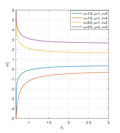
(a) $e_{\alpha,\varphi_{1}}(X)$ with Normal prior distribution

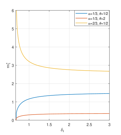
(b) $e_{\alpha,\varphi_{1}}(Y)$ with Exponential prior distribution

Figure 1: The effect of penalization function $\varphi_{1}$ on $e_{\alpha,\varphi_{1}}$ under different distributions

3.2 Robust expectiles with $\varphi_{2}$

This subsection considers the second specific penalization function $\varphi_{2}(x)=\infty I_{(\delta_{2},+\infty)}(x)$, $x\geq 0$, with $\delta_{2}>0$. It is named by the robust expectiles with $\varphi_{2}$. For any $\mu$ in $\mathcal{M}(\mathbb{R})$, $\varphi_{2}(d_{c}\left(\mu_{X},\mu\right))=\infty$ if $d_{c}\left(\mu_{X},\mu\right)>\delta_{2}$, which means the potential uncertainty distributions $\mu$ of $X$ should satisfy $d_{c}\left(\mu_{X},\mu\right)\leq\delta_{2}$.

Definition 3.2.

Suppose $X\in L^{2}(\Omega,\mathcal{F},P)$. For any $\alpha\in(0,1)$, let $h$ be the loss function defined by (6). The cost function $c(x,y)=|x-y|^{2}$. Then the robust expectiles with penalization function $\varphi_{2}$ are defined by:

$$e_{\alpha,\varphi_{2}}(X):=\underset{m\in\mathbb{R}}{\operatorname{argmin}}~{}\mathcal{E}_{\varphi_{2}}(h,X,m).$$

Proposition 3.2.

Let $\alpha\in(0,1)$, and $e_{\alpha,\varphi_{2}}(X)$ be the robust expectiles of $X$, Then

$$e_{\alpha,\varphi_{2}}(X)=\underset{m\in\mathbb{R}}{\operatorname{argmin}}\left\{\inf_{\lambda>max\{\alpha,1-\alpha\}}g_{2}(X,m,\lambda,\alpha)\right\},$$

where

$$g_{2}(X,m,\lambda,\alpha)=\frac{\alpha\lambda}{\lambda-\alpha}E_{P}\left[((X-m)^{+})^{2}\right]+\frac{(1-\alpha)\lambda}{\lambda-(1-\alpha)}E_{P}\left[((X-m)^{-})^{2}\right]+\delta_{2}\lambda.$$

Obviously, for the given random variable $X$ and $\alpha$, $g_{2}(X,m,\lambda,\alpha)$ is a binary convex function with respect to $(m,\lambda)$. To obtain the optimal solution when it reaches its extreme value, we give the partial derivatives of $g_{2}(X,m,\lambda,\alpha)$ with respect to $m$ and $\lambda$ respectively,

$$\frac{\partial g_{2}(X,m,\lambda,\alpha)}{\partial\lambda}=-\frac{\alpha^{2}}{(\lambda-\alpha)^{2}}E_{P}\left[((X-m)^{+})^{2}\right]-\frac{(1-\alpha)^{2}}{(\lambda-1+\alpha)^{2}}E_{P}\left[((X-m)^{-})^{2}\right]+\delta_{2},$$

$$\frac{\partial g_{2}(X,m,\lambda,\alpha)}{\partial m}=-\frac{2\alpha\lambda}{\lambda-\alpha}E_{P}\left[(X-m)^{+}\right]+\frac{2(1-\alpha)\lambda}{\lambda-1+\alpha}E_{P}\left[(X-m)^{-}\right].\hskip 60.00009pt$$

It is noting that when $\delta_{2}=0$, one has that

$$\frac{\partial g_{2}(X,m,\lambda,\alpha)}{\partial\lambda}\leq 0,$$

which implies that $g_{2}(X,m,\lambda,\alpha)$ is decreasing about $\lambda$. Hence, $g_{2}(X,m,\lambda,\alpha)$ reaches the minimum value at $\lambda\rightarrow+\infty$, it follows that

$$\inf_{\lambda>max\{\alpha,1-\alpha\}}~{}g_{2}(X,m,\lambda,\alpha)~{} =\lim_{\lambda\to+\infty}g_{2}(X,m,\lambda,\alpha)$$

$$=\alpha E_{P}\left[((X-m)^{+})^{2}\right]+(1-\alpha)E_{P}\left[((X-m)^{-})^{2}\right].$$

Hence, the minimization problem reduces to

$$\underset{m\in\mathbb{R}}{\operatorname{argmin}}\Big{\{}\alpha E_{P}\left[((X-m)^{+})^{2}\right]+(1-\alpha)E_{P}\left[((X-m)^{-})^{2}\right]\Big{\}},$$

which is exactly the expectiles.

Remark 3.2.

For $\varphi_{2}(x)=\infty I_{(\delta_{2},+\infty)}(x)$, it means that we consider only those distributions that satisfy $d_{c}\left(\mu_{X},\mu\right)\leq\delta_{2}$. If we take $\delta_{2}=0$, it implies that we only consider the distribution of uncertain future losses to be deterministic and be $\mu_{X}$. Hence, the robust expectiles lead to the classical expectiles without uncertainty distributions.

Now, let’s think about the case where $\delta_{2}>0$, one has that

$$\lim_{\lambda\rightarrow max\{\alpha,1-\alpha\}}\frac{\partial g_{2}(X,m,\lambda,\alpha)}{\partial\lambda}=-\infty;\hskip 3.00003pt\lim_{\lambda\rightarrow+\infty}\frac{\partial g_{2}(X,m,\lambda,\alpha)}{\partial\lambda}=\delta_{2}>0.$$

Hence, we know that there exist constants $m_{2}^{*}\in\mathbb{R}$ and $\lambda^{*}>max\{\alpha,1-\alpha\}$, such that

$$\left\{\begin{aligned} \frac{\partial g_{2}(X,m,\lambda,\alpha)}{\partial\lambda}\bigg{|}_{m=m_{2}^{*},~{}\lambda=\lambda^{*}}=0,\\ \frac{\partial g_{2}(X,m,\lambda,\alpha)}{\partial m}\bigg{|}_{m=m_{2}^{*},~{}\lambda=\lambda^{*}}=0,\\ \end{aligned}\right.$$

and $m_{2}^{*}$ is the robust expectile $e_{\alpha,\varphi_{2}}(X)$.

In the following, we will investigate the impact of the penalization function on $e_{\alpha,\varphi_{2}}$ for the specific prior distribution.

Figure 2 depicts the $e_{\alpha,\varphi_{2}}$ with different prior distributions and different parameters of prior distributions. Contrary to $e_{\alpha,\varphi_{1}}$, when $\alpha\in(\frac{1}{2},1)$, $e_{\alpha,\varphi_{2}}$ is increasing with respect to $\delta_{2}$, while if $\alpha\in(0,\frac{1}{2})$, $e_{\alpha,\varphi_{2}}$ is decreasing with respect to $\delta_{2}$. Similarly, the degree of changes becomes slower with the increase of $\delta_{2}$. This is because no matter whether we use the penalization functions $\varphi_{1}$ or $\varphi_{2}$, it tends to be that those distributions far away from the baseline distribution should not have a major impacts on our results.

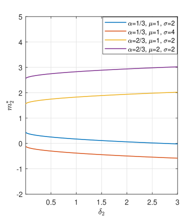
(a) $e_{\alpha,\varphi_{2}}(X)$ with Normal prior distribution

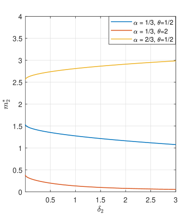
(b) $e_{\alpha,\varphi_{2}}(Y)$ with Exponential prior distribution

Figure 2: The effect of penalization function $\varphi_{2}$ on $e_{\alpha,\varphi_{2}}$ under different prior distributions

3.3 Comparisons with expectiles

According to Figure 1 and Figure 2, we have analyzed the influence of the coefficient of the penalization functions on robust expectiles under normal distribution and exponential distribution. In fact, the change trends of robust expectiles with respect to $\delta_{1}$ or $\delta_{2}$ under the $T$ distribution are similarly consistent with that under the normal distribution. This subsection considers the differences between the classical expectiles and the robust expectiles under $T$ distribution.

Figure 3 indicates the impact on expectiles after introducing nonlinear expectation with penalty. It reveals that the trends of $e_{\alpha,\varphi_{2}}$, $e_{\alpha,\varphi_{1}}$ and expectiles with respect to $\alpha$ are the similar. For $e_{\alpha,\varphi_{1}}$, it is always smaller than the expectiles when $\alpha\in(0,\frac{1}{2}]$, and it has already known that $e_{\alpha,\varphi_{1}}$ is increasing with respect $\delta_{1}$, which implies that the larger $\delta_{1}$ is, the closer $e_{\alpha,\varphi_{1}}$ is to the expectiles. While $e_{\alpha,\varphi_{1}}$ is always bigger than the expectiles when $\alpha\in[\frac{1}{2},1)$, and $e_{\alpha,\varphi_{1}}$ is decreasing with respect $\delta_{1}$, which can also implies that the larger $\delta_{1}$ is, the closer $e_{\alpha,\varphi_{1}}$ is to the expectiles.

However, it is different for $e_{\alpha,\varphi_{2}}$. We find that the larger $\delta_{2}$ is, the farther away $e_{\alpha,\varphi_{2}}$ is from the expectiles. This is because for $e_{\alpha,\varphi_{2}}$, the larger $\delta_{2}$ means the more distributions are considered, and the more deviations from the expectiles should be expected.

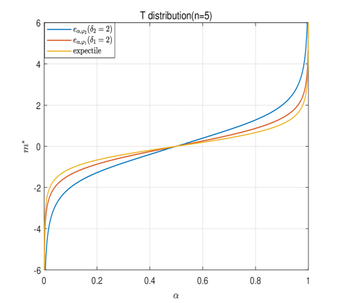
Figure 3: The comparisons between robust expectiles and expectiles under $T$ prior distribution.

4 The Proofs

This section provides the proofs of the previous propositions and theorems. In the following, we will use the duality theorem obtained by Bartl, Drapeau and Tangpi (2020).

Lemma 4.1.

(Bartl, Drapeau and Tangpi (2020), Theorem 2.7) The following duality theorem holds, i.e., for any random variable $X$,

$$\mathcal{OCE}_{l,\varphi}(X)=\inf_{\lambda\geq 0}\left\{OCE_{l^{\lambda c}}(X)+\varphi^{*}(\lambda)\right\},$$ (7)

with

$$OCE_{l^{\lambda c}}(X)=\inf_{m\in\mathbb{R}}\left\{m+\int_{\mathbb{R}}l^{\lambda c}(x-m)\mu_{X}(dx)\right\}=\inf_{m\in\mathbb{R}}\left\{m+E_{P}[l^{\lambda c}(X-m)]\right\},$$ (8)

where $l$ is a loss function, $\varphi^{*}$ is the convex conjugate of a penalization function $\varphi$ and $l^{\lambda c}$ is $\lambda c$-transform for $l$, which is defined by

$$l^{\lambda c}(x):=\sup_{y\in\mathbb{R}}\{l(y)-\lambda|x-y|^{p}\},~{}~{}x\in\mathbb{R}.$$

Lemma 4.2.

Let a loss function $l(\cdot):\mathbb{R}\to\mathbb{R}$ be convex and increasing. Then for any $\lambda\geq 0$, the $\lambda c$-transform for the loss function $l$ has the following properties:

• $l^{\lambda c}(x)\geq l(x)$ for any $x\in\mathbb{R}$;

• $l^{\lambda c}(x)$ is increasing with respect to $x$;

• $l^{\lambda c}(x)$ is convex with respect to $(x,\lambda).$

Proof.  By substitution of variables, for any $\lambda\geq 0$, the $\lambda c$-transform can be expressed as

$$l^{\lambda c}(x)=\sup_{y\in\mathbb{R}}\left\{l(x-y)-\lambda|y|^{p}\right\},~{}~{}\forall x\in\mathbb{R}.$$

Hence, $(a)$ obviously holds. Since the loss function $l$ is increasing, it implies that $(b)$ is true.

To the part $(c)$, for any $t\in(0,1)$, $x_{1},x_{2}\in\mathbb{R}$ and $\lambda_{1},\lambda_{2}\geq 0$, since the loss function $l(\cdot)$ is convex, it follows that

$$l^{(t\lambda_{1}+(1-t)\lambda_{2})c}(tx_{1}+(1-t)x_{2})$$

$$=~{} \sup_{y\in\mathbb{R}}\left\{l(tx_{1}+(1-t)x_{2}-y)-(t\lambda_{1}+(1-t)\lambda_{2})|y|^{p}\right\}$$

$$\leq~{} \sup_{y\in\mathbb{R}}\{tl(x_{1}-y)+(1-t)l(x_{2}-y)-(t\lambda_{1}+(1-t)\lambda_{2})|y|^{p}\}$$

$$\leq~{} t\sup_{y\in\mathbb{R}}\{l(x_{1}-y)-\lambda_{1}|y|^{p}\}+(1-t)\sup_{y\in\mathbb{R}}\{l(x_{2}-y)-\lambda_{2}|y|^{p}\}$$

$$=~{} tl^{\lambda_{1}c}(x_{1})+(1-t)l^{\lambda_{2}c}(x_{2}).$$

$\Box$

Proof of Proposition 2.1. The prior distribution invariance property $(a)$ is obvious derived from the definition of $\mathcal{OCE}_{l,\varphi}(\cdot)$.

For any random variable $X$, by Lemma 4.1, we obtain that

$$\mathcal{OCE}_{l,\varphi}(X)=\inf_{\lambda\geq 0}\left\{OCE_{l^{\lambda c}}(X)+\varphi^{*}(\lambda)\right\},$$

with $OCE_{l^{\lambda c}}(X)=\inf_{m\in\mathbb{R}}\left\{m+E_{P}[l^{\lambda c}(X-m)]\right\}.$ Therefore, for any $C\in\mathbb{R}$,

$$OCE_{l^{\lambda c}}(X+C) =\inf_{m\in\mathbb{R}}\left\{m+E_{P}[l^{\lambda c}(X+C-m)]\right\}$$

$$=\inf_{m_{1}\in\mathbb{R}}\left\{m_{1}+C+E_{P}[l^{\lambda c}(X-m_{1})]\right\}$$

$$=OCE_{l^{\lambda c}}(X)+C.$$

It means that $(b)$ holds.

If $X\leq Y$,$P$-a.s., since $l$ is increasing, by Lemma 4.2, we know that the $\lambda c$-transform $l^{\lambda c}(\cdot)$ is increasing, then it implies that

$$OCE_{l^{\lambda c}}(X)\leq OCE_{l^{\lambda c}}(Y).$$

Hence, $\mathcal{OCE}_{l,\varphi}(X)\leq\mathcal{OCE}_{l,\varphi}(Y),$ i.e., $(c)$ is true.

Since $l(\cdot)$ is convex, Lemma 4.2 leads to $l^{\lambda c}(x)$ is convex with respect to $(x,\lambda)$. Therefore, for any $t\in(0,1)$, random variables $X,Y$ and $\lambda_{1},\lambda_{2}\geq 0$,

$$\hskip 20.00003ptOCE_{l^{(t\lambda_{1}+(1-t)\lambda_{2})c}}(tX+(1-t)Y)$$

$$=\inf_{m_{1},m_{2}\in\mathbb{R}}\left\{tm_{1}+(1-t)m_{2}+E_{P}[l^{(t\lambda_{1}+(1-t)\lambda_{2})c}(tX+(1-t)Y-(tm_{1}+(1-t)m_{2}))]\right\}$$

$$\leq t\inf_{m_{1}\in\mathbb{R}}\left\{m_{1}+E_{P}[l^{\lambda_{1}c}(X-m_{1})]\right\}+(1-t)\inf_{m_{2}\in\mathbb{R}}\left\{m_{2}+E_{P}[l^{\lambda_{1}c}(Y-m_{2})]\right\}$$

$$=tOCE_{l^{\lambda_{1}c}}(X)+(1-t)OCE_{l^{\lambda_{2}c}}(Y).$$ (9)

On the other hand, since $\varphi^{*}$ is the convex conjugate of the penalization function $\varphi$, then $\varphi^{*}(\cdot)$ is convex. Combing the the convexity of OCE in (4), it implies that

$$\mathcal{OCE}_{l,\varphi}(tX+(1-t)Y) =\inf_{\lambda\geq 0}\left\{OCE_{l^{\lambda c}}(tX+(1-t)Y)+\varphi^{*}(\lambda)\right\}$$

$$=\inf_{\lambda_{1},\lambda_{2}\geq 0}\left\{OCE_{l^{(t\lambda_{1}+(1-t)\lambda_{2})c}}(tX+(1-t)Y)+\varphi^{*}(t\lambda_{1}+(1-t)\lambda_{2})\right\}$$

$$\leq t\inf_{\lambda_{1}\geq 0}\left\{OCE_{l^{\lambda_{1}c}}(X)+\varphi^{*}(\lambda_{1})\right\}+(1-t)\inf_{\lambda_{2}\geq 0}\left\{OCE_{l^{\lambda_{2}c}}(Y)+\varphi^{*}(\lambda_{2})\right\}$$

$$=t\mathcal{OCE}_{l,\varphi}(X)+(1-t)\mathcal{OCE}_{l,\varphi}(Y).$$

Thus, $\mathcal{OCE}_{l,\varphi}(\cdot)$ is convex. The proof is complete. $\Box$

Proof of Proposition 2.3

By Lemma 4.1, we obtain that

$$\mathcal{OCE}_{l,\varphi}(X)=\inf_{\lambda\geq 0}\left\{OCE_{l^{\lambda c}}(X)+\varphi^{*}(\lambda)\right\},$$

with $OCE_{l^{\lambda c}}(X)=\inf_{m\in\mathbb{R}}\left\{m+E_{P}[l^{\lambda c}(X-m)]\right\}.$

Since $\Lambda_{l}(X,\varphi)\neq\emptyset$, one has that

$$\mathcal{OCE}_{l,\varphi}(X) =\inf_{\lambda\geq 0}\left\{OCE_{l^{\lambda c}}(X)+\varphi^{*}(\lambda)\right\}$$

$$=\inf_{\lambda\in\Lambda_{l}(X,\varphi)}\left\{OCE_{l^{\lambda c}}(X)+\varphi^{*}(\lambda)\right\}.$$ (10)

For any $\lambda\in\Lambda_{l}(X,\varphi)$, let $F(m)=m+E_{P}[l^{\lambda c}(X-m)]$. Then we only need to consider those $m$ that make $F(m)<+\infty$. In this case, since $suppX=[x_{min},x_{max}]$ with $-\infty<x_{min}\leq x_{max}<+\infty$, by Lebesgue’s dominated convergence theorem, we can freely interchange integration with one-sided derivation. Hence, one has that

$$F^{{}^{\prime}}_{+}(m)=1-E_{P}[(l^{\lambda c})^{{}^{\prime}}_{+}(X-m)]\textrm{~{}~{}and~{}~{}}F^{{}^{\prime}}_{-}(m)=1-E_{P}[(l^{\lambda c})^{{}^{\prime}}_{-}(X-m)].$$

Since $l$ is convex, which leads to $F(m)$ is convex in $m$. If $m^{*}$ is the optimal solution of $OCE_{l^{\lambda c}}(X)$, then it should be

$$F^{{}^{\prime}}_{-}(m^{*})\leq 0\leq F^{{}^{\prime}}_{+}(m^{*}).$$

Then, one has that

$$E_{P}[(l^{\lambda c})^{{}^{\prime}}_{-}(X-m^{*})]\leq 1\leq E_{P}[(l^{\lambda c})^{{}^{\prime}}_{+}(X-m^{*})].$$

Next, we prove there exists $m^{*}\in suppX$. If $m^{*}<x_{min}$, then $X-m^{*}>X-x_{min}$. Since $l\in L(X,\varphi)$ and $l^{\lambda c}(\cdot)$ is convex, which leads to $(l^{\lambda c})^{{}^{\prime}}_{+}$ and $(l^{\lambda c})^{{}^{\prime}}_{-}$ are nondecreasing, we can obtain that

$$1\geq E_{P}[(l^{\lambda c})^{{}^{\prime}}_{-}(X-m^{*})]\geq E_{P}[(l^{\lambda c})^{{}^{\prime}}_{+}(X-x_{min})]\geq E_{P}[(l^{\lambda c})^{{}^{\prime}}_{-}(X-x_{min})]\geq(l^{\lambda c})^{{}^{\prime}}_{+}(0).$$

Similarly, if $m^{*}>x_{max}$, we can obtain

$$(l^{\lambda c})^{{}^{\prime}}_{-}(0)\geq E_{P}[(l^{\lambda c})^{{}^{\prime}}_{+}(X-x_{max})]\geq E_{P}[(l^{\lambda c})^{{}^{\prime}}_{-}(X-x_{max})]\geq E_{P}[(l^{\lambda c})^{{}^{\prime}}_{+}(X-m^{*})]\geq 1.$$

Since $l\in L(X,\varphi)$, then for any $\lambda\in\Lambda_{l}(X,\varphi)$, $l^{\lambda c}(x)\geq l^{\lambda c}(0)+x$ for all $x\in\mathbb{R}$, and $l^{\lambda c}(\cdot)$ is convex, one has that

$$(l^{\lambda c})^{{}^{\prime}}_{+}(0)\geq 1\geq(l^{\lambda c})^{{}^{\prime}}_{-}(0),$$

which leads to that

$$E_{P}[(l^{\lambda c})^{{}^{\prime}}_{+}(X-x_{min})]=E_{P}[(l^{\lambda c})^{{}^{\prime}}_{-}(X-x_{min})]=1,$$

or

$$E_{P}[(l^{\lambda c})^{{}^{\prime}}_{+}(X-x_{max})]=E_{P}[(l^{\lambda c})^{{}^{\prime}}_{-}(X-x_{max})]=1.$$

Hence, $x_{min}$ or $x_{max}$ is the optimal solution of $OCE_{l^{\lambda c}}(X)$. This is a contradiction.

Therefore, for any $\lambda\in\Lambda_{l}(X,\varphi)$, we have

$$OCE_{l^{\lambda c}}(X)=\min_{m\in suppX}\left\{m+E_{P}[l^{\lambda c}(X-m)]\right\}.$$

Then, according to (4), one has that

$$\mathcal{OCE}_{l,\varphi}(X) =\inf_{\lambda\in\Lambda_{l}(X,\varphi)}\left\{\min_{m\in suppX}\left\{m+E_{P}[l^{\lambda c}(X-m)]\right\}+\varphi^{*}(\lambda)\right\}$$

$$=\inf_{\lambda\geq 0}\left\{\min_{m\in suppX}\left\{m+E_{P}[l^{\lambda c}(X-m)]\right\}+\varphi^{*}(\lambda)\right\}$$

$$=\min_{m\in suppX}\left\{m+\inf_{\lambda\geq 0}\left\{\varphi^{*}(\lambda)+E_{P}[l^{\lambda c}(X-m)]\right\}\right\}$$

$$=\min_{m\in suppX}\left\{m+\mathcal{E}_{\varphi}(l,X,m)\right\}.$$

$\Box$

Proof of Proposition 2.4

$(a)$ Since $l_{1}$ and $l_{2}$ are convex, then for each $x$, $h(x-m)$ is convex in $m$. Hence, for each $t\in(0,1)$, for all $m_{1},m_{2}\in\mathbb{R}$,

$$\hskip 20.00003pt\mathcal{E}_{\varphi}(h,X,tm_{1}+(1-t)m_{2}))$$

$$=\sup_{\mu\in\mathcal{M}(\mathbb{R})}\left(\int_{\mathbb{R}}h(x-(tm_{1}+(1-t)m_{2}))\mu(dx)-\varphi\left(d_{c}\left(\mu_{X},\mu\right)\right)\right)$$

$$\leq\sup_{\mu\in\mathcal{M}(\mathbb{R})}\left(t\int_{\mathbb{R}}h(x-m_{1})\mu(dx)+(1-t)\int_{\mathbb{R}}h(x-m_{2})d\mu-\varphi\left(d_{c}\left(\mu_{X},\mu\right)\right)\right)$$

$$\leq t\sup_{\mu\in\mathcal{M}(\mathbb{R})}\left(\int_{\mathbb{R}}h(x-m_{1})\mu(dx)-\varphi\left(d_{c}\left(\mu_{X},\mu\right)\right)\right)$$

$$+(1-t)\sup_{\mu\in\mathcal{M}(\mathbb{R})}\left(\int_{\mathbb{R}}h(x-m_{2})\mu(dx)-\varphi\left(d_{c}\left(\mu_{X},\mu\right)\right)\right)$$

$$=t\mathcal{E}_{\varphi}(h,X,m_{1})+(1-t)\mathcal{E}_{\varphi}(h,X,m_{2}),$$

which implies $\mathcal{E}_{\varphi}(h,X,m)$ is convex about $m$.

On the other hand, from the definition of $\mathcal{E}_{\varphi}(h,X,m)$, it follows that

$$\mathcal{E}_{\varphi}(h,X,m) =\sup_{\mu\in\mathcal{M}(\mathbb{R})}\left(\int_{\mathbb{R}}h(x-m)\mu(dx)-\varphi\left(d_{c}\left(\mu_{X},\mu\right)\right)\right)$$

$$\geq E_{P}[\alpha l_{1}((X-m)^{+})+(1-\alpha)l_{2}((X-m)^{-})].$$

Since the monotonicity and convexity properties of the loss functions $l_{1}$ and $l_{2}$, then by the monotone convergence theorem, it derives

$$\lim_{m\rightarrow-\infty}E_{P}\left[\alpha l_{1}((X-m)^{+})+(1-\alpha)l_{2}((X-m)^{-})\right]=+\infty,$$

and

$$\lim_{m\rightarrow+\infty}E_{P}\left[\alpha l_{1}((X-m)^{+})+(1-\alpha)l_{2}((X-m)^{-})\right]=+\infty.$$

Hence, one has that

$$\lim_{m\rightarrow-\infty}\mathcal{E}_{\varphi}(h,X,m)=\lim_{m\rightarrow+\infty}\mathcal{E}_{\varphi}(h,X,m)=+\infty.$$

$(b)$ Since $\mathcal{E}_{\varphi}(h,X,0)<+\infty$, then it implies $\underset{m\in\mathbb{R}}{\operatorname{inf}}~{}\mathcal{E}_{\varphi}(h,X,m)<+\infty$. Due to the facts that $\mathcal{E}_{\varphi}(h,X,m)$ is convex about $m$ and $\lim_{m\rightarrow\pm\infty}\mathcal{E}_{\varphi}(h,X,m)=+\infty$, then it is easy to find that there exists a closed interval $[m_{1},m_{2}]$, such that

$$[m_{1},m_{2}]=\underset{m\in\mathbb{R}}{\operatorname{argmin}}~{}\hskip 1.00006pt\mathcal{E}_{\varphi}(h,X,m).$$

$\Box$

Proof of Lemma 2.1

Since $h$ has polynomial growth, it means there exists a constant $C\geq 0$ such that for all $x\in\mathbb{R}$, $h(x)\leq C(1+|x|^{p})$, then it implies that, for each $\lambda\geq 0$ and $x\in\mathbb{R}$,

$$\sup_{y\in\mathbb{R}}\{h(y)-\lambda|x-y|^{p}\} \leq\sup_{y\in\mathbb{R}}\{C(1+|y|^{p})-\lambda|x-y|^{p}\}.$$

Obviously, there exists a $\lambda^{*}>C$, such that $h^{\lambda^{*}c}(x)<+\infty$ for all $x\in\mathbb{R}$. $\Box$

Proof of Proposition 2.5

For any $\alpha\in(0,1)$, $m\in\mathbb{R}$, then

$$h(x-m)=\alpha(x-m)^{+}+(1-\alpha)(x-m)^{-},~{}~{}\forall x\in\mathbb{R}.$$

It is obvious that $h(\cdot-m)$ is bounded from below. Based on Lemma 4.1, we can obtain the $\lambda c$-transform of $h(\cdot-m)$. Directly calculations, it derives that

$$h^{\lambda c}(x-m)=\begin{cases}\alpha(x-m)^{+}+(1-\alpha)(x-m)^{-},&\text{ if }\lambda\geq max\{\alpha,1-\alpha\},\\ +\infty,&\text{ if }\lambda<max\{\alpha,1-\alpha\},\end{cases}$$

where $\varphi^{*}$ is the convex conjugate for the penalization function $\phi$. Then,

$$\mathcal{E}_{\varphi}(h,X,m)=\inf_{\lambda\geq max\{\alpha,1-\alpha\}}\{E_{P}\left[\alpha(X-m)^{+}+(1-\alpha)(X-m)^{-}\right]+\varphi^{*}(\lambda)\}.$$

Since $\varphi^{*}(\lambda)$ is increasing with respect to $\lambda$, then

$$\mathcal{E}_{\varphi}(h,X,m)=E_{P}\left[\alpha(X-m)^{+}+(1-\alpha)(X-m)^{-}\right]+\varphi^{*}(max\{\alpha,1-\alpha\}).$$

Hence, it obvious that

$$\underset{m\in\mathbb{R}}{\operatorname{argmin}}\left\{\mathcal{E}_{\varphi}(h,X,m)\right\}=\underset{m\in\mathbb{R}}{\operatorname{argmin}}\{\alpha E_{P}\left[(X-m)^{+}\right]+(1-\alpha)E_{P}\left[(X-m)^{-}\right]\}.$$

By Exercise 4.4.1 in Föllmer and Schied (2016), its optimal solution $m^{*}\in\underset{m\in\mathbb{R}}{\operatorname{argmin}}\mathcal{E}_{\varphi}(h,X,m)$ satisfies

$$P(X<m^{*})\leq\alpha\leq P(X\leq m^{*}).$$

It is exactly the $VaR_{\alpha}(X)$ in the classical situation, which means $q_{\alpha,\varphi}(X)=VaR_{\alpha}(X)$. $\Box$

Proof of Proposition 3.1

For each $\alpha\in(0,1)$ and $m\in\mathbb{R}$, denote

$$h(x-m)=\alpha((x-m)^{+})^{2}+(1-\alpha))((x-m)^{-})^{2},\forall x\in\mathbb{R}.$$

Then, the $\lambda c$-transform of loss function $h(\cdot-m)$ can be calculated as follows and it can be divided into three cases.

Case (i): When $\alpha\in(0,\frac{1}{2})$, then

$$h^{\lambda c}(x-m)=\begin{cases}+\infty,&\text{ if }\lambda<1-\alpha,\\ \\ \frac{\alpha(1-\alpha)}{1-2\alpha}((x-m)^{+})^{2}+\infty I_{(-\infty,m)}(x),&\text{ if }\lambda=1-\alpha,\\ \\ \frac{\alpha\lambda}{\lambda-\alpha}((x-m)^{+})^{2}+\frac{(1-\alpha)\lambda}{\lambda-(1-\alpha)}((x-m)^{-})^{2},&\text{ if }\lambda>1-\alpha.\end{cases}$$

Case (ii): When $\alpha=\frac{1}{2}$, then

$$h^{\lambda c}(x-m)=\begin{cases}+\infty,&\text{ if }\lambda\leq\frac{1}{2},\\ \\ \frac{\alpha\lambda}{\lambda-\alpha}((x-m)^{+})^{2}+\frac{(1-\alpha)\lambda}{\lambda-(1-\alpha)}((x-m)^{-})^{2},&\text{ if }\lambda>\frac{1}{2}.\end{cases}$$

Case (iii): When $\alpha\in(\frac{1}{2},1)$, then

$$h^{\lambda c}(x-m)=\begin{cases}+\infty,&\text{ if }\lambda<\alpha,\\ \\ \infty I_{(m,+\infty)}(x)+\frac{(1-\alpha)\alpha}{2\alpha-1}((x-m)^{-})^{2},&\text{ if }\lambda=\alpha,\\ \\ \frac{\alpha\lambda}{\lambda-\alpha}((x-m)^{+})^{2}+\frac{(1-\alpha)\lambda}{\lambda-(1-\alpha)}((x-m)^{-})^{2},&\text{ if }\lambda>\alpha.\end{cases}$$

Since $\varphi_{1}(x)=\delta_{1}x$ , one has that $\varphi_{1}^{*}(\lambda)=\infty I_{(\delta_{1},+\infty)}(\lambda)$. Therefore, by Lemma 4.1, it follows that

$$\mathcal{E}_{\varphi_{1}}(h,X,m) =\sup_{\mu\in\mathcal{M}(\mathbb{R})}\left(\int_{\mathbb{R}}h(x-m)\mu(dx)-\delta_{1}d_{c}\left(\mu_{X},\mu\right)\right)$$

$$=\inf_{\lambda\geq 0}\left\{E_{P}[h^{\lambda c}(X-m)]+\infty I_{(\delta_{1},+\infty)}(\lambda)\right\}$$

$$=\inf_{0\leq\lambda\leq\delta_{1}}~{}E_{P}[h^{\lambda c}(X-m)]$$

$$=\inf_{max\{\alpha,1-\alpha\}<\lambda\leq\delta_{1}}g_{1}(X,m,\lambda,\alpha),$$

where

$$g_{1}(X,m,\lambda,\alpha)=\frac{\alpha\lambda}{\lambda-\alpha}E_{P}\left[((X-m)^{+})^{2}\right]+\frac{(1-\alpha)\lambda}{\lambda-(1-\alpha)}E_{P}\left[((X-m)^{-})^{2}\right].$$

It is clear that $g_{1}(X,m,\lambda,\alpha)$ is decreasing with respect to $\lambda$. Thus, one has that

$$\inf_{max\{\alpha,1-\alpha\}<\lambda\leq\delta_{1}}g_{1}(X,m,\lambda,\alpha)=g_{1}(X,m,\delta_{1},\alpha).$$

$\Box$

Proof of Theorem 3.1. For any $\alpha\in(\frac{1}{2},1)$ and $\delta_{1}>\alpha$, we verify that $e_{\alpha,\varphi_{1}}(\cdot)$ satisfies the axioms of the coherent risk measures.

(i) Translation invariance. For any constants $C$ and $m$ in $\mathbb{R}$, since

$$g_{1}(X+C,m,\delta_{1},\alpha)=g_{1}(X,m-C,\delta_{1},\alpha).$$

Hence, by the definition of robust expectile, then it implies that

$$e_{\alpha,\varphi_{1}}(X+C)=e_{\alpha,\varphi_{1}}(X)+C.$$

(ii) Monotonicity. Since $X\in L^{2}(\Omega,\mathcal{F},P)$, then it can be verified that $g_{1}(X,m,\delta_{1},\alpha)$ is differentiable with respect to $m$, and

$$g_{1}^{\prime}(X,m,\delta_{1},\alpha)=-\frac{2\alpha\delta_{1}}{\delta_{1}-\alpha}E_{P}\left[(X-m)^{+}\right]+\frac{2(1-\alpha)\delta_{1}}{\delta_{1}-(1-\alpha)}E_{P}\left[(X-m)^{-}\right],~{}\forall m\in\mathbb{R}.$$

Since $e_{\alpha,\varphi_{1}}(X)=\underset{m\in\mathbb{R}}{\operatorname{argmin}}~{}g_{1}(X,m,\delta_{1},\alpha)$ and $g_{1}(X,\cdot,\delta_{1},\alpha)$ is convex, then its optimal value for $m$ should satisfy

$$g_{1}^{\prime}(X,m,\delta_{1},\alpha)=0.$$

Since $\delta_{1}>max\{\alpha,1-\alpha\}$, one has that

$$-\frac{2\alpha\delta_{1}}{\delta_{1}-\alpha}<0~{}~{}\textrm{and}~{}~{}\frac{2(1-\alpha)\delta_{1}}{\delta_{1}-(1-\alpha)}>0.$$

Then, for the given $\delta_{1},m$ and $\alpha$, $g_{1}^{\prime}(X,m,\delta_{1},\alpha)$ is decreasing with respect to $X$, i.e., if $X\leq Y$, $P$-a.s., then $g_{1}^{\prime}(X,m,\delta_{1},\alpha)\geq g_{1}^{\prime}(Y,m,\delta_{1},\alpha)$.

Therefore, when $X\leq Y$, $P$-a.s., then

$$g_{1}^{\prime}(Y,e_{\alpha,\varphi_{1}}(X),\delta_{1},\alpha)\leq g_{1}^{\prime}(X,e_{\alpha,\varphi_{1}}(X),\delta_{1},\alpha)=0.$$

Since $g_{1}^{\prime}(Y,m,\delta_{1},\alpha)$ is increasing with respect to $m$, and $g_{1}^{\prime}(Y,e_{\alpha,\varphi_{1}}(Y),\delta_{1},\alpha)=0$, then it implies that

$$e_{\alpha,\varphi_{1}}(X)\leq e_{\alpha,\varphi_{1}}(Y).$$

(iii) Convexity. Since $\alpha\in(\frac{1}{2},1)$ and $\delta_{1}>max\{\alpha,1-\alpha\}$, then it can derive that

$$\frac{2\alpha\delta_{1}}{\delta_{1}-\alpha}\geq\frac{2(1-\alpha)\delta_{1}}{\delta_{1}-(1-\alpha)},$$

which inplies that $g_{1}^{\prime}(X,m,\delta_{1},\alpha)$ is concave with respect to $(X,m)$. Recall that

$$g_{1}^{\prime}(X,e_{\alpha,\varphi_{1}}(X),\delta_{1},\alpha)=0\textrm{ and }g_{1}^{\prime}(Y,e_{\alpha,\varphi_{1}}(Y),\delta_{1},\alpha)=0.$$

For any $t\in(0,1)$, it then implies

$$g_{1}^{\prime}\left(tX+(1-t)Y,te_{\alpha,\varphi_{1}}(X)+(1-t)e_{\alpha,\varphi_{1}}(Y),\delta_{1},\alpha\right)$$

$$\geq ~{}tg_{1}^{\prime}\left(X,e_{\alpha,\varphi_{1}}(X),\delta_{1},\alpha\right)+(1-t)g_{1}^{\prime}\left(Y,e_{\alpha,\varphi_{1}}(Y),\delta_{1},\alpha\right)$$

$$= 0.$$

Since $g_{1}^{\prime}(X,m,\delta_{1},\alpha)$ is increasing with respect to $m$, and

$$g_{1}^{\prime}(tX+(1-t)Y,e_{\alpha,\varphi_{1}}(tX+(1-t)Y),\delta_{1},\alpha)=0.$$

Therefore, for the given random variables $X$ and $Y$, for each $t\in(0,1)$, $\alpha\in(\frac{1}{2},1)$, and $\delta_{1}>max\{\alpha,1-\alpha\}$, then

$$e_{\alpha,\varphi_{1}}(tX+(1-t)Y)\leq te_{\alpha,\varphi_{1}}(X)+(1-t)e_{\alpha,\varphi_{1}}(Y).$$

(iv) Positive homogeneity. When $t=0$, it is obvious that $e_{\alpha,\varphi_{1}}(0)=0$. For any $t>0$, one has that

$$g_{1}^{\prime}(tX,m,\delta_{1},\alpha)=tg_{1}^{\prime}(X,\frac{m}{t},\delta_{1},\alpha).$$

Hence, for any $t\geq 0$, $e_{\alpha,\varphi_{1}}(tX)=t\hskip 1.99997pte_{\alpha,\varphi_{1}}(X)$. $\Box$

Proof of Theorem 3.2

Suppose $\alpha\in(\frac{1}{2},1)$. By Theorem 3.1, $e_{\alpha,\varphi_{1}}(X)$ is also a convex risk measure. Based on Proposition 4.113 and Theorem 4.115 in Föllmer and Schied (2016), $e_{\alpha,\varphi_{1}}(X)$ can be represented as

$$e_{\alpha,\varphi_{1}}(X)=\underset{Q\in\mathcal{M}(P_{X})}{\operatorname{max}}\left\{E_{Q}[X]-\inf_{t>0}\frac{1}{t}E_{P}\left[\psi^{*}(t\frac{\mathrm{d}Q}{\mathrm{d}P})\right]\right\},$$

where

$$\mathcal{M}(P)=\left\{Q:Q\textrm{ is absolutely continuous with respect to }P\right\},$$

and $\psi^{*}$ is the dual conjugate function of $\psi$ with

$$\psi^{*}(x)=\begin{cases}0&\text{ }\frac{2(1-\alpha)\delta_{1}}{\delta_{1}-(1-\alpha)}\leq x\leq\frac{2\alpha\delta_{1}}{\delta_{1}-\alpha},\\ +\infty&\text{ }else.\\ \end{cases}$$

Hence, it derives that

$$\inf_{t>0}\frac{1}{t}E_{P}[\psi^{*}(t\frac{\mathrm{d}Q}{\mathrm{d}P})]=\begin{cases}0&\exists t_{0}>0,s.t.,\frac{2(1-\alpha)\delta_{1}}{\delta_{1}-(1-\alpha)}\leq t_{0}\frac{\mathrm{d}Q}{\mathrm{d}P}\leq\frac{2\alpha\delta_{1}}{\delta_{1}-\alpha},\\ +\infty&\text{ }else.\\ \end{cases}$$

Thus, $e_{\alpha,\varphi_{1}}(X)=\underset{\mu\in\mathcal{M}_{1}(P)}{\operatorname{max}}E_{Q}[X]$.

Since $e_{\alpha,\varphi_{1}}(X)=-e_{1-\alpha,\varphi_{1}}(-X)$, it is easy to obtain the dual representation of $e_{\alpha,\varphi_{1}}(X)$ when $\alpha\in(0,\frac{1}{2})$. $\Box$

Proof of Proposition 3.2

Since $\varphi_{2}(x)=\infty I_{(\delta_{2},+\infty)}(x)$, then the convex conjugate function of $\varphi_{2}$ is

$$\varphi_{2}^{*}(y)=\delta_{2}y^{+},~{}~{}y\in\mathbb{R}.$$

By Lemma 4.1, it implies that

$$\mathcal{E}_{2}(h,X,m) =\sup_{\mu\in\mathcal{M}(\mathbb{R}),d_{c}(\mu_{X},\mu)\leq\delta_{2}}\int_{\mathbb{R}}h(x-m)\mu(dx)$$

$$=\inf_{\lambda\geq 0}\left\{E_{P}[h^{\lambda c}(X-m)]+\delta_{2}\lambda\right\}$$

$$=\inf_{\lambda>max\{\alpha,1-\alpha\}}g_{2}(X,m,\lambda),$$

where $h^{\lambda c}$ can be found in Proposition 3.1. We complete the proof. $\Box$

5 The Conclusions

Inspired by Bartl, Drapeau and Tangpi (2020), the paper analyzes the relevant properties of the robust optimized certainty equivalents as risk measures for loss positions with distribution uncertainty. Based on the robust optimized certainty equivalents, we propose the robust generalized quantiles, which is a natural generalization for the quantiles. Furthermore, we focus on two kinds of specific robust expectiles corresponding to two penalization functions $\varphi_{1}$ and $\varphi_{2}$. The robust expectiles with $\varphi_{1}$ are proved to be coherent risk measures, and the dual representation theorems are established. The results are a development and complement to Bellini et al. (2014) and Bartl, Drapeau and Tangpi (2020). Besides, we also study the influences of penalization functions on the robust expectiles and compare them with expectiles for some specific prior distributions by numerical simulations.

References

- Acerbi (2002) Acerbi, C., 2002. Spectral measures of risk: a coherent representation of subjective risk aversion. J. Bank Financ., 26, 1505-1518.
- Acerbi and Tasche (2002) Acerbi, C., Tasche, D., 2002. On the coherence of expected shortfall. J. Bank Financ., 26, 1487-1503.
- Artzner et al. (1997) Artzner, Ph., Delbaen, F., Eber, J.M., Heath, D., 1997. Thinking coherently. Risk, 10, 71-86.
- Artzner et al. (1999) Artzner, Ph., Delbaen, F., Eber, J.M., Heath, D., 1999. Coherent measures of risk. Mathematical Finance, 4, 203-228.
- Breckling and Chambers (1988) Breckling, J., Chambers, R., 1988. M-quantiles. Biometrika, 75, 761-772.