Testing CP-violation in a Heavy Higgs Sector at CLIC

Abstract

We propose a novel method to test CP-violation in the heavy (pseudo)scalar sector of an extended Higgs model, in which we make simultaneous use of the $HVV$ ($V=W^{\pm},Z$) and $Ht\bar{t}$ interactions of a heavy Higgs state $H$. This is possible at the Compact Linear Collider (CLIC) by exploiting $H$ production from Vector-Boson Fusion (VBF) and decay to $t\bar{t}$ pairs. We analyze the distribution of the azimuthal angle between the leptons coming from top and antitop quarks, that would allow one to disentangle the CP nature of such a heavy Higgs state. We also show its implications for the 2-Higgs-Doublet Model (2HDM) with CP-violation.

I Introduction

CP-violation was first discovered in the long-lived $K$-meson rare decay channel $K_{L}\rightarrow 2\pi$ in 1964 Christenson:1964fg . More CP-violation effects were also measured in the $K$-, $D$- and $B$-meson sectors in the past several decades Aaij:2019kcg ; Zyla:2020zbs ; Workman:2022ynf (see Khalil:2022toi for a historical review). All these measured CP-violation effects are consistent with the explanation given through the Kobayashi-Maskawa (KM) mechanism Kobayashi:1973fv , which represents another success of the Standard Model (SM) of particle physics. However, it is necessary to search for CP-violation sources Beyond the SM (BSM). One important reason to do so is that the amount of CP-violation contained in the SM is not enough to explain the matter-antimatter asymmetry in the Universe Cohen:1991iu ; Cohen:1993nk ; Morrissey:2012db .

Theoretically, many BSM scenarios can accommodate additional CP-violation sources to remedy such a flaw of the SM. However, the latter are strongly constrained by experiments. Specifically, measurements of the Electric Dipole Moments (EDMs) of, e.g., electron and neutron Andreev:2018ayy ; Cairncross:2017fip ; Abel:2020gbr have already set stringent limits on such new sources (or else could reveal their existence) Engel:2013lsa ; Yamanaka:2017mef ; Safronova:2017xyt ; Chupp:2017rkp , as the sensitivities involved are far above the SM predictions Pospelov:2005pr ; Yamaguchi:2020eub ; Yamaguchi:2020dsy . However, the EDM measurements, being very inclusive, are only an “indirect” probe of such new CP-violation sources, which means that, even if we discovered herein CP-violation above the SM predictions, it is unlikely that we could determine the actual interactions involved. Conversely, collider experiments, despite having weaker sensitivities to CP-violation in comparison to EDM ones, can afford one, thanks to the vast variety of exclusive observables that one can define herein, with a “direct” probe of CP-violation.

The case for the complementarity of these two experimental settings can easily be made for BSM frameworks with extended Higgs sectors Bento:1991ez ; Lee:1973iz ; Lee:1974jb ; Branco:2011iw ; Weinberg:1976hu . As an example, Ref. Cheung:2020ugr studied both EDM and collider effects in a 2-Higgs Doublet Model (2HDM) Branco:2011iw with explicit CP-violation, in which non-zero EDMs are expected to be the first signal of it with collider effects able to provide additional information.

After the discovery of the 125 GeV Higgs boson at the Large Hadron Collider (LHC) Aad:2012tfa ; Chatrchyan:2012xdj ; Aad:2015zhl , testing its CP properties is crucial to ascertain the structure of the underlying Higgs sector. On the one hand, current measurements are consistent with the CP-even (or scalar) state of the SM. On the other hand, an additional Higgs state, possibly mixing with it, may have different CP-properties (e.g., being pseudoscalar or a mixture of the two). To stay with 2HDMs, in these BSM scenarios, an effective method to test the CP-properties of the ensuing physical states is trying to test CP-violation effects in the Yukawa interactions between such an additional (heavy) Higgs boson and fermions via the Lagrangian term

$$\mathcal{L}\supset-\bar{f}\left(g_{S}+\textrm{i}g_{P}\gamma^{5}\right)fH.$$ (1)

Usually, $f=t$ or $\tau$, because a top quark or $\tau$ lepton decays quickly enough so that the CP-properties and spin information of the decaying object is protected in its final state distributions. In fact, the spin and CP quantum numbers correlate strongly in the Yukawa interaction. Phenomenologically, there are a lot of works in literature trying to test CP-violation in $Ht\bar{t}$ Schmidt:1992et ; Mahlon:1995zn ; Asakawa:2003dh ; BhupalDev:2007ftb ; He:2014xla ; Boudjema:2015nda ; Buckley:2015vsa ; AmorDosSantos:2017ayi ; Azevedo:2017qiz ; Bernreuther:2017cyi ; Hagiwara:2017ban ; Ma:2018ott ; Cepeda:2019klc ; Faroughy:2019ird ; Cheung:2020ugr ; Cao:2020hhb ; Azevedo:2020fdl ; Azevedo:2020vfw or $H\tau^{+}\tau^{-}$ Desch:2003rw ; Berge:2008wi ; Harnik:2013aja ; Berge:2013jra ; Berge:2014sra ; Berge:2015nua ; Askew:2015mda ; Hagiwara:2016zqz ; Jozefowicz:2016kvz ; Antusch:2020ngh ; Kanemura:2021atq interactions at colliders.

Besides this, one can also probe CP-violation in the purely bosonic sector, through the interactions between a Higgs state and the SM massive gauge bosons. To exploit this approach, we again need such an additional Higgs state $H$ (while the SM-like $125$ GeV Higgs boson is denoted as $h$). The general effective interactions among $h$, $H$ and $V=W,Z$ are (with $\theta_{W}$ being the weak mixing angle)

$$\mathcal{L}\supset\left(\frac{2m^{2}_{W}}{v}W^{+,\mu}W^{-}_{\mu}+\frac{m^{2}_{Z}}{v}Z^{\mu}Z_{\mu}\right)\left(c_{h}h+c_{H}H\right)+\frac{c_{hH}g}{2c_{\theta_{W}}}Z^{\mu}\left(h\partial_{\mu}H-H\partial_{\mu}h\right).$$ (2)

We already know that $c_{h}\neq 0$ through current LHC measurements. If both $c_{H}$ and $c_{hH}$ are non-zero, we will confirm CP-violation in the Higgs sector because in such a case $h$ and $H$ cannot be CP eigenstates at the same time, as was shown in Li:2016zzh ; Mao:2017hpp ; Mao:2018kfn .

In the SM, as hinted above, the only CP-violation source is the complex phase in the Cabibbo-Kobayashi-Maskawa (CKM) matrix Kobayashi:1973fv , which means that, if there exists new CP-violation in Higgs interactions, the Higgs sector of the SM must be extended. Consequently, it becomes attractive to search for CP-violation through the dynamics of additional Higgs states, as done recently for 2HDMs, both fundamental and composite, in Refs. Azevedo:2020fdl ; Azevedo:2020vfw ; Antusch:2020ngh ; Kanemura:2021atq ; DeCurtis:2021uqx , which indeed exploited either $Ht\bar{t}$ or $HVV$ couplings.

In this paper, we propose a novel method to test CP-violation through such a heavy $H$ state, as we consider its interactions with both massive fermions and gauge bosons simultaneously. The advantage of this approach is that the CP-even component in $H$ is confirmed through $HVV$ ($V=W^{\pm},Z$) interactions while the CP-odd component in $H$ is confirmed through $Ht\bar{t}$ interaction. In order to do so, we consider a process in which the heavy Higgs state $H$ is produced through Vector Bosons Fusion (VBF), i.e., $W^{+}W^{-}$- or $ZZ$-fusion, and decays into top (anti)quark pairs ($t\bar{t}$). As collider setup, we choose an electron-positron one, in preference to a hadronic one, because of the cleanliness of the described signature therein and, amongst the various future options for the latter, we privilege the Compact Linear Collider (CLIC) design Linssen:1425915 ; Lebrun:1475225 ; Abramowicz:2016zbo ; Aicheler:2018arh ; CLIC:2018fvx ; CLICdp:2018cto ; Brunner:2022usy because its $\sqrt{s}$ can reach $\mathcal{O}(\textrm{TeV})$, hence, comparable to the LHC reach.

The paper is organized as follows. We describe our method in Sec. II using a model-independent formulation. In Sec. III, as an illustration, we apply it to the 2HDM with CP-violation. Finally, we conclude in Sec. IV.

II Model-independent Studies

II.1 Method

Assuming a heavy scalar $H$ is discovered, and in this paper we focus on the CP properties of this particle. Its effective interactions with massive gauge bosons and fermions can be written in general as

$$\mathcal{L}\supset c_{V}H\left(\frac{2m^{2}_{W}}{v}W^{+,\mu}W^{-}_{\mu}+\frac{m^{2}_{Z}}{v}Z^{\mu}Z_{\mu}\right)-\mathop{\sum}_{f}\frac{m_{f}}{v}H\bar{f}\left[\textrm{Re}\left(c_{f}\right)+\textrm{i}\textrm{Im}\left(c_{f}\right)\gamma^{5}\right]f.$$ (3)

We choose the VBF processes $VV\rightarrow H\rightarrow t\bar{t}$ where $V=W^{\pm}$ or $Z$, and the Feynman diagrams are shown in Fig. 1.

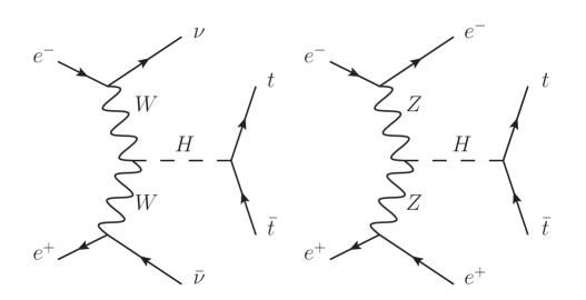
Figure 1: The Feynman diagrams for VBF processes $VV\rightarrow H\rightarrow t\bar{t}$ where $V=W^{\pm},Z$.

If such processes can be measured, we have $c_{V}\neq 0$ and thus the CP-even component of $H$ will be confirmed. For the final state $t\bar{t}$, if $\textrm{Im}\left(c_{t}\right)=0$ and $\textrm{Re}\left(c_{t}\right)\neq 0$, meaning it is a pure scalar, the $t\bar{t}$ pair will form in a ${}^{3}P_{0}$ state. Instead, if $\textrm{Re}\left(c_{t}\right)=0$ and $\textrm{Im}\left(c_{t}\right)\neq 0$, meaning it is a pure pseudoscalar, the $t\bar{t}$ pair will form a ${}^{1}S_{0}$ state. In the CP-violation scenario, there will be both ${}^{3}P_{0}$ and ${}^{1}S_{0}$ types of $t\bar{t}$ final states. Thus, the spin correlation behavior between the top and antitop quarks is sensitive to the CP nature of Higgs states in Yukawa interactions.

We choose semi-leptonic decay channels $t\left(\bar{t}\right)\rightarrow b\ell^{+}\nu\left(\bar{b}\ell^{-}\bar{\nu}\right)$ ($\ell=e,\mu$) for both top and antitop quarks. The azimuthal angle between $\ell^{+}$ and $\ell^{-}$ (denoted as $\Delta\phi$) is a good observable to measure the spin correlations between top and antitop quarks Mahlon:2010gw ; ATLAS:2012ao ; Baumgart:2012ay ; Ellis:2013yxa ; Mileo:2016mxg ; Aguilar-Saavedra:2018ggp , hence, it is helpful to probe CP-violation in the Yukawa sector . For example, we show the normalized distributions of the azimuthal angle $\Delta\phi$ (denoted as $\frac{1}{\sigma}\frac{d\sigma}{d\Delta\phi}$) between the charged leptons from $t\bar{t}$ at CLIC with $\sqrt{s}=1.5~{}\textrm{TeV}$ in Fig. 2 for both the $W^{+}W^{-}$- and $ZZ$-fusion channels.

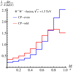
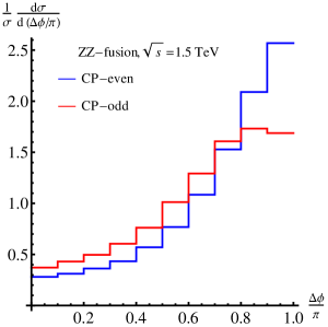
Figure 2: Normalized distributions of the azimuthal angle $\Delta\phi$ (denoted as $\frac{1}{\sigma}\frac{d\sigma}{d(\Delta\phi/\pi)}$) between the charged leptons from $t\bar{t}$ at CLIC with $\sqrt{s}=1.5~{}\textrm{TeV}$ for both the $W^{+}W^{-}$-fusion (the left plot) and $ZZ$-fusion (the right plot) channels. The blue lines are for a CP-even $Ht\bar{t}$ coupling, while the red lines are for a CP-odd $Ht\bar{t}$ coupling.

It is clear to see that the $\Delta\phi$ distributions are different between the cases with CP-even and CP-odd $Ht\bar{t}$ couplings, for both $W^{+}W^{-}$- and $ZZ$-fusion channels. As discussed above, VBF production implies the existence of the CP-even component in $H$ and, from the $\Delta\phi$ distribution, if we can find the evidence of a non-zero $\textrm{Im}\left(c_{t}\right)$ (or equivalently the ${}^{1}S_{0}$ type $t\bar{t}$ final state), we can confirm also the CP-odd component in $H$, and hence the CP-violation effects. Such a method will prove to be more effective for a heavy scalar $H$ mainly containing the CP-odd component, as this is the most different one from the SM background.

II.2 Simulation Studies at CLIC

We choose two cases: CLIC with $\sqrt{s}=1.5~{}\textrm{TeV}$ and $3~{}\textrm{TeV}$ separately. We further choose $c_{V}$ not larger than $0.3$, because the global-fit for the 125 GeV Higgs boson data implies $c_{V}\lesssim 0.3$ . The direct LHC search for a heavy scalar $H$ decaying to $ZZ$ final states sets further limits on $c_{V}$ if $m_{H}\lesssim 700~{}\textrm{GeV}$ ATLAS:2020tlo , so that we choose the LHC-favored region with a benchmark point having $m_{H}=700~{}\textrm{GeV}$.

In our simulation studies, we consider two VBF processes at CLIC: $W^{+}W^{-}$ fusion ($e^{+}e^{-}\rightarrow\nu\overline{\nu}H$) and $ZZ$ fusion ($e^{+}e^{-}\rightarrow e^{+}e^{-}H$), with the heavy Higgs $H$ decaying to a $t\bar{t}$ pair with top quark and antiquark decaying semileptonically. We assume that the heavy Higgs $H$ can decay via only three channels: $H\rightarrow t\overline{t}$, $W^{+}W^{-}$ and $ZZ$. The Branching Ratio (BR) for the $H\rightarrow t\bar{t}$ decay channel

$$\textrm{BR}_{H\rightarrow t\bar{t}}\equiv\frac{\Gamma_{H\rightarrow t\bar{t}}}{\Gamma_{H\rightarrow t\bar{t}}+\Gamma_{H\rightarrow W^{+}W^{-}}+\Gamma_{H\rightarrow ZZ}}$$ (4)

thus depends on the couplings $c_{V}$ and $c_{t}$, where Branco:2011iw

$$\Gamma_{H\rightarrow t\bar{t}} = \frac{3m_{H}}{8\pi}\left(\frac{m_{t}}{v}\right)^{2}\left[\left[\textrm{Re}(c_{t})\right]^{2}\left(1-\frac{4m^{2}_{t}}{m^{2}_{H}}\right)^{\frac{3}{2}}+\left[\textrm{Im}(c_{t})\right]^{2}\left(1-\frac{4m^{2}_{t}}{m^{2}_{H}}\right)^{\frac{1}{2}}\right],$$ (5)

$$\Gamma_{H\rightarrow W^{+}W^{-}} = \frac{m_{H}^{3}c_{V}^{2}}{16\pi v^{2}}\sqrt{1-\frac{4m^{2}_{W}}{m^{2}_{H}}}\left(1-\frac{4m^{2}_{W}}{m^{2}_{H}}+\frac{12m^{4}_{W}}{m^{4}_{H}}\right),$$ (6)

$$\Gamma_{H\rightarrow ZZ} = \frac{m_{H}^{3}c_{V}^{2}}{32\pi v^{2}}\sqrt{1-\frac{4m^{2}_{Z}}{m^{2}_{H}}}\left(1-\frac{4m^{2}_{Z}}{m^{2}_{H}}+\frac{12m^{4}_{Z}}{m^{4}_{H}}\right).$$ (7)

As we choose $m_{H}=700~{}\textrm{GeV}$ in our simulation studies, the $\textrm{BR}_{H\rightarrow t\bar{t}}$ has the following numerical dependence on $c_{V}$ and $c_{t}$:

$$\textrm{Br}_{H\rightarrow t\bar{t}}=\frac{0.174\left[\textrm{Re}(c_{t})\right]^{2}+0.229\left[\textrm{Im}(c_{t})\right]^{2}}{c_{V}^{2}+0.174\left[\textrm{Re}(c_{t})\right]^{2}+0.229\left[\textrm{Im}(c_{t})\right]^{2}}.$$ (8)

In Eq. 5, the term proportional to $\left[\textrm{Re}(c_{t})\right]^{2}$ implies that the partial decay width to $t\bar{t}$ pairs involves a ${}^{3}P_{0}$ state, while the term proportional to $\left[\textrm{Im}(c_{t})\right]^{2}$ implies that the partial decay width to $t\bar{t}$ pairs involves a ${}^{1}S_{0}$ state. The branching ratio of the top quark semileptonic decay is chosen as $21.34\%$, which is the sum of electron and muon channels, as shown in the Particle Data Group (PDG) review Workman:2022ynf . In our simulation studies, we generate the signal and background events at the Leading Order (LO) order using MadGraph5 Alwall:2014hca . We include bremsstrahlung/Initial State Radiation (ISR) effects through the “isronlyll” option for Parton Distribution Function (PDFs) Frixione:2021zdp .

In the $W^{+}W^{-}$-fusion channel, the main background is the SM $s$-channel $t\overline{t}$ production because of its large production rate (and the fact that the (anti)neutrinos in the final state of the signal cannot be triggered on) while other background processes are numerically negligible. In the $ZZ$-fusion channel, the main background is instead SM $t\overline{t}e^{+}e^{-}$ production, which comes from both the VBF production process of $t\overline{t}$ and the $t\overline{t}Z$ associated production process with the $Z$ boson decaying to an electron pair. To reduce the SM backgrounds, we apply the selection cuts in Table 1.

Table 1: Selection cuts for $W^{+}W^{-}$- and $ZZ$-fusion processes at CLIC with $\sqrt{s}=1.5~{}\textrm{TeV}$ (the upper two entries) and $\sqrt{s}=3~{}\textrm{TeV}$ (the lower two entries).

Process	Selection cuts
$W^{+}W^{-}$-fusion ($\sqrt{s}=1.5~{}\textrm{TeV}$)	$n_{\ell}=2,~{}n_{b}=2,~{}\mid\eta^{\ell}\mid<3,~{}\mid\eta^{b}\mid<5,$ $p_{\textrm{T}}^{\ell,b}>10~{}\mbox{GeV},~{}p_{\textrm{T}}^{\mbox{\tiny miss}}<300~{}\mbox{GeV},~{}\Delta R_{\ell\ell,b\ell,bb}>0.4,$ $m_{bb\ell\ell}<600~{}\mbox{GeV},~{}m_{\ell\ell}<350~{}\mbox{GeV},~{}m_{\mbox{\tiny inv}}>850~{}\mbox{GeV}.$
$ZZ$-fusion ($\sqrt{s}=1.5~{}\textrm{TeV}$)	$n_{\ell}\geq 3,~{}n_{e}\geq 1,~{}n_{\ell^{+}}\cdot n_{\ell^{-}}>0,~{}n_{b}=2,$ $\mid\eta^{\ell}\mid<3,~{}\mid\eta^{b}\mid<5,~{}\textrm{max}(\mid\eta^{\ell}\mid)>2,~{}\Delta R_{\ell\ell,b\ell,bb}>0.4,$ $p_{\mathrm{T}}^{\ell,b}>10~{}\mbox{GeV},~{}m_{bb\ell\ell}>350~{}\mbox{GeV},~{}m_{\mbox{\tiny inv}}<400~{}\mbox{GeV}.$
$W^{+}W^{-}$-fusion ($\sqrt{s}=3~{}\textrm{TeV}$)	$n_{\ell}=2,~{}n_{b}=2,~{}\mid\eta^{\ell}\mid<3,~{}\mid\eta^{b}\mid<5,$ $p_{\mathrm{T}}^{\ell,b}>10~{}\mbox{GeV},~{}p_{\mathrm{T}}^{\mbox{\tiny miss}}<150~{}\mbox{GeV},~{}p_{\mathrm{T}}^{\ell\ell}<200~{}\mbox{GeV},~{}\Delta R_{\ell\ell,b\ell,bb}>0.4,$ $m_{bb\ell\ell}<700~{}\mbox{GeV},~{}m_{\ell\ell}<450~{}\mbox{GeV},~{}m_{\mbox{\tiny inv}}>1900~{}\mbox{GeV}.$
$ZZ$-fusion ($\sqrt{s}=3~{}\textrm{TeV}$)	$n_{\ell}\geq 3,~{}n_{e}\geq 1,~{}n_{\ell^{+}}\cdot n_{\ell^{-}}>0,~{}n_{b}=2,$ $\mid\eta^{\ell}\mid<3,~{}\mid\eta^{b}\mid<5,~{}\textrm{max}(\mid\eta^{\ell}\mid)>2,$ $\Delta R_{\ell\ell,b\ell,bb}>0.4,~{}p_{\mathrm{T}}^{\ell,b}>10~{}\mbox{GeV},~{}m_{bb\ell\ell}>350~{}\mbox{GeV}.$

After performing these selection cuts, we have the cross sections $\sigma_{i}$ and the corresponding selection efficiencies $\epsilon$ for the signal (denoted as the index “sig”) and background (denoted as the index “bkg”) processes in Table 2 together with the discovery potential as a function of the machine luminosity $L$.

Table 2: Cross sections after selection cuts, selection efficiencies and expected significance for $W^{+}W^{-}$- and $ZZ$-fusion processes at CLIC with $\sqrt{s}=1.5~{}\textrm{TeV}$ (the upper two entries) and $\sqrt{s}=3~{}\textrm{TeV}$ (the lower two entries). Here, $N_{\textrm{sig}}=\sigma_{\textrm{sig}}L$ and $N_{\textrm{bkg}}=\sigma_{\textrm{bkg}}L$ are separately the event rates for signal and background after selection cuts, while $L$ is the integrated luminosity.

Process	$\sigma_{\textrm{sig}}$ (fb)	$\epsilon_{\textrm{sig}}$	$\sigma_{\textrm{bkg}}$ (fb)	$\epsilon_{\textrm{bkg}}$	$N_{\textrm{sig}}/\sqrt{N_{\textrm{bkg}}}$
$W^{+}W^{-}$-fusion ($\sqrt{s}=1.5~{}\textrm{TeV}$)	$~{}~{}~{}0.94\kappa~{}~{}~{}$	$~{}~{}~{}64\%~{}~{}~{}$	$~{}~{}~{}0.34~{}~{}~{}$	$~{}~{}~{}8.4\%~{}~{}~{}$	$~{}~{}~{}1.6\times 10^{2}\kappa\sqrt{L/(10~{}\textrm{ab}^{-1})}~{}~{}~{}$
$ZZ$-fusion ($\sqrt{s}=1.5~{}\textrm{TeV}$)	$~{}~{}~{}0.088\kappa~{}~{}~{}$	$~{}~{}~{}61\%~{}~{}~{}$	$0.013$	$~{}~{}~{}36\%~{}~{}~{}$	$~{}~{}~{}78\kappa\sqrt{L/(10~{}\textrm{ab}^{-1})}~{}~{}~{}$
$W^{+}W^{-}$-fusion ($\sqrt{s}=3~{}\textrm{TeV}$)	$~{}~{}~{}4.14\kappa~{}~{}~{}$	$~{}~{}~{}62\%~{}~{}~{}$	$~{}~{}~{}0.041~{}~{}~{}$	$~{}~{}~{}3.6\%~{}~{}~{}$	$~{}~{}~{}2.0\times 10^{3}\kappa\sqrt{L/(10~{}\textrm{ab}^{-1})}~{}~{}~{}$
$ZZ$-fusion ($\sqrt{s}=3~{}\textrm{TeV}$)	$~{}~{}~{}0.28\kappa~{}~{}~{}$	$~{}~{}~{}42\%~{}~{}~{}$	$~{}~{}~{}0.019~{}~{}~{}$	$~{}~{}~{}21\%~{}~{}~{}$	$~{}~{}~{}2.0\times 10^{2}\kappa\sqrt{L/(10~{}\textrm{ab}^{-1})}~{}~{}~{}$

For the rates in the table, we know that the signal production cross sections are proportional to the parameter

$$\kappa\equiv\frac{c_{V}^{2}\left(0.174\left[\textrm{Re}(c_{t})\right]^{2}+0.229\left[\textrm{Im}(c_{t})\right]^{2}\right)}{c_{V}^{2}+0.174\left[\textrm{Re}(c_{t})\right]^{2}+0.229\left[\textrm{Im}(c_{t})\right]^{2}}=c_{V}^{2}\textrm{Br}_{H\rightarrow t\bar{t}}.$$ (9)

Since $c_{V}\lesssim 0.3$ Cheung:2020ugr , if we fix $|c_{t}|=1$, the largest allowed number for this parameter should be $\kappa_{\textrm{max}}^{+}=0.059$ for a CP-even $Ht\bar{t}$ coupling and $\kappa_{\textrm{max}}^{-}=0.065$ a for CP-odd $Ht\bar{t}$ coupling. If we choose as typical integrated luminosity $L=10~{}\textrm{ab}^{-1}$ and the largest allowed $c_{V}=0.3$, in all the four cases, the signal $VV\rightarrow H\rightarrow t(\rightarrow b\ell^{+}\nu)\bar{t}(\rightarrow\bar{b}\ell^{-}\bar{\nu})$ will be discovered with its significance close to or larger than $5\sigma$ for both CP-even and CP-odd $Ht\bar{t}$ couplings quite promptly at CLIC, so that we have the basis to further analyze the final state $\Delta\phi$ distributions to probe the CP nature of the $H$ state.

II.3 Analysis and Results

For all the four cases (both $W^{+}W^{-}$- and $ZZ$-fusion, with $\sqrt{s}=1.5~{}\textrm{TeV}$ and $3~{}\textrm{TeV}$), we show the $\Delta\phi$ distribution in Fig. 3, including both signal and background events.

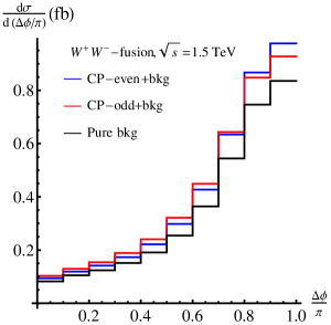
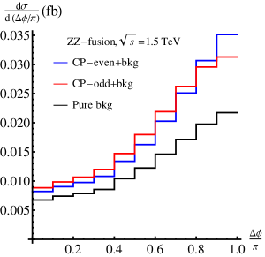
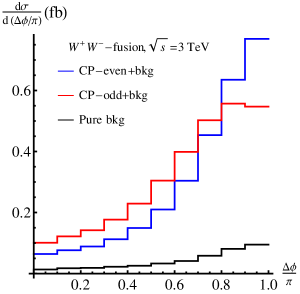
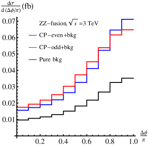
Figure 3: Differential cross sections in the azimuthal angle $\Delta\phi$ [denoted as $\frac{d\sigma}{d(\Delta\phi/\pi)}$] between the charged leptons from $t\bar{t}$ at CLIC including both signal and background events: the upper plots are for the case with $\sqrt{s}=1.5~{}\textrm{TeV}$ and the lower plots are for the case with $\sqrt{s}=3~{}\textrm{TeV}$ while the left plots are for the $W^{+}W^{-}$-fusion process and the right plots are for the $ZZ$-fusion process. The blue lines are for a CP-even $Ht\bar{t}$ coupling together with background events while the red lines are for a CP-odd $Ht\bar{t}$ coupling together with background events while we also show the distribution for pure background events as black lines.

We also add the $\Delta\phi$ distribution for pure background events for comparison. The plots clearly show differences between the two CP hypothese in the $\Delta\phi$ distribution even after adding the background events.

We then define the forward-backward asymmetry as

$${A}\equiv\frac{N_{\Delta\phi>\pi/2}-N_{\Delta\phi<\pi/2}}{N_{\Delta\phi>\pi/2}+N_{\Delta\phi<\pi/2}}=\frac{N_{+}-N_{-}}{N_{+}+N_{-}},$$ (10)

which is sensitive to the CP nature of the $Ht\bar{t}$ coupling. Its uncertainty can be calculated through

$$\sigma_{{A}}=\sqrt{\frac{4N_{+}N_{-}}{N^{3}}},$$ (11)

where $N=N_{+}+N_{-}$ is the total number of events. In our analysis, for all the cases, we must consider the signal and background events together, since they become indistinguishable experimentally even after our selection cuts. Thus, $N_{\pm}$ contains both signal and background events.

We calculate such a forward-backward asymmetry for each process (denoted through the sub-indices $W^{+}W^{-}$ and $ZZ$ in the plots) for both pure CP-even $(+)$ and pure CP-odd $(-)$ $Ht\bar{t}$ couplings, hence, we use ${A}^{\pm}$ (in the forthcoming text), together with their $\pm 1\sigma$ uncertainties $\sigma_{{A}^{\pm}}$ assuming as integrated luminosity $L=10~{}\textrm{ab}^{-1}$, and show the results in Fig. 4. In the calculation, we always fix $[\textrm{Re}(c_{t})]^{2}+1.32[\textrm{Re}(c_{t})]^{2}=1$ as a benchmark point, so that the parameter $\kappa$ defined in Eq. 9 becomes $\kappa=0.174c_{V}^{2}/(c_{V}^{2}+0.174)$ and the total cross sections do not depend on $\arg(c_{t})=\arctan[\textrm{Im}(c_{t})/\textrm{Re}(c_{t})]$.

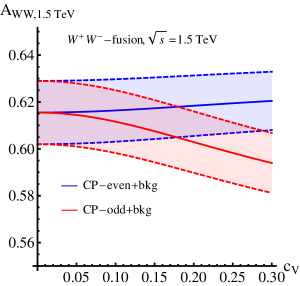
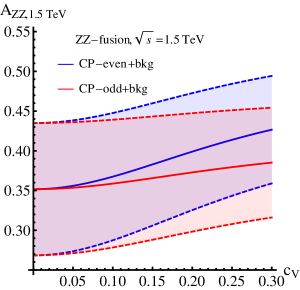
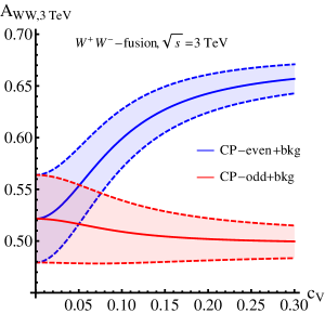
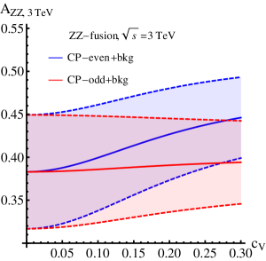
Figure 4: Forward-backward asymmetries ${A}$ including both signal and background events: the upper plots are for the case with $\sqrt{s}=1.5~{}\textrm{TeV}$ and the lower plots are for the case with $\sqrt{s}=3~{}\textrm{TeV}$ while the left plots are for the $W^{+}W^{-}$-fusion process and the right plots are for the $ZZ$-fusion process. We fix $[\textrm{Re}(c_{t})]^{2}+1.32[\textrm{Re}(c_{t})]^{2}=1$ for all processes. The blue lines are for ${A}^{+}$ including background events while the red lines are for ${A}^{-}$ including background events. The solid lines are the central values ${A}^{\pm}$ while the dashed lines are ${A}^{\pm}\pm\sigma_{{A}^{\pm}}$, where $\sigma_{{A}^{\pm}}$ are the $1\sigma$ uncertainties for ${A}^{\pm}$ for the integrated luminosity $L=10~{}\textrm{ab}^{-1}$.

For the case with CP-mixing $Ht\bar{t}$ coupling, the forward-backward asymmetry will be located between blue and red lines. In our method, a non-zero $\textrm{Im}(c_{t})$ is enough to probe CP-violation, thus we choose a pure CP-odd $Ht\bar{t}$ coupling to find the largest deviation from the CP-conserving case (CP-even). For given experimental conditions and model parameters, the number of standard deviation

$$s_{0}=\frac{|{A}-{A}^{+}|}{\sigma_{{A}^{+}}}$$ (12)

away from the CP-conserving case measures the significance to discover CP-violation, so that, for a pure CP-odd $Ht\bar{t}$ coupling, we have ${A}={A}^{-}$, which will give us the largest significance for CP-violation.

From the right plots in Fig. 4, it is clear that in the $ZZ$-fusion channel, it is difficult to distinguish between a CP-even and CP-odd $Ht\bar{t}$ coupling. Even for the largest allowed value $c_{V}=0.3$, we still have $s_{0}$ less than or close to $1$, meaning that ${A}^{-}$ is quite close to ${A}^{+}$. That is mainly because of the small cross section and hence event number of the $ZZ$-fusion process, in turn affecting adversely the error. Thus, for $ZZ$-fusion, we do not need further analysis. For $W^{+}W^{-}$-fusion with $\sqrt{s}=1.5~{}\textrm{TeV}$ and upon choosing the largest allowed $c_{V}=0.3$, $s_{0}\simeq 2.1$ meaning a slight deviation can be found but still not an evidence strong enough to discover CP-violation. That is because at the $\sqrt{s}=1.5~{}\textrm{TeV}$ CLIC, there is still large $t\bar{t}$ background which cannot be reduced effectively, i.e., $\sigma_{\textrm{bkg}}\gg\sigma_{\textrm{sig}}$. The large background erases the difference between ${A}^{+}$ and ${A}^{-}$ and thus only a $2.1\sigma$ deviation is left even for $c_{V}=0.3$. We do not analyze this case further then. For $W^{+}W^{-}$-fusion with $\sqrt{s}=3~{}\textrm{TeV}$, from the lower-left plot in Fig. 4, if $c_{V}\gtrsim 0.1$, we have $s_{0}\gtrsim 3$ meaning that ${A}^{-}$ and ${A}^{+}$ are significantly different in this case.

Therefore, we discuss the $W^{+}W^{-}$-fusion process further at CLIC with $\sqrt{s}=3~{}\textrm{TeV}$. Experimentally, the two useful observables are the total cross section $\sigma_{\textrm{tot}}=\sigma_{\textrm{sig}}+\sigma_{\textrm{bkg}}$ and the forward-backward asymmetry ${A}$ in the $\Delta\phi$ distribution. Notice that $\sigma_{\textrm{tot}}$ depends only on the parameter $\kappa$ while ${A}$ depends on both $\kappa$ and $\xi\equiv\arg(c_{t})$. Numerically, we have

$$\sigma_{\textrm{tot}} = \sigma_{\textrm{sig}}+\sigma_{\textrm{bkg}}=(4.14\kappa+0.041)~{}\textrm{fb},$$ (13)

$${A} = \frac{1}{\sigma_{\textrm{tot}}}\left({A}_{\textrm{bkg}}\sigma_{\textrm{bkg}}+{A}^{+}\sigma_{\textrm{sig}}\frac{c^{2}_{\xi}}{c^{2}_{\xi}+1.32s^{2}_{\xi}}+{A}^{-}\sigma_{\textrm{sig}}\frac{1.32s^{2}_{\xi}}{c^{2}_{\xi}+1.32s^{2}_{\xi}}\right)$$ (14)

$$= \frac{1}{\kappa+9.8\times 10^{-3}}\left(5.1\times 10^{-3}+\frac{0.68c^{2}_{\xi}+0.65s^{2}_{\xi}}{c^{2}_{\xi}+1.32s^{2}_{\xi}}\kappa\right).$$

With a luminosity $L=10~{}\textrm{ab}^{-1}$, the relative uncertainty of $\sigma_{\textrm{tot}}$ is determined by $\delta\sigma_{\textrm{tot}}/\sigma_{\textrm{tot}}=1/\sqrt{N_{\textrm{sig}}+N_{\textrm{bkg}}}\sim\mathcal{O}(10^{-2})$ , which is ignorable compared with the relative uncertainty of ${A}$. In Fig. 5, we show the correlation between asymmetry ${A}$ and total cross section $\sigma_{\textrm{tot}}$ for different $\xi$ in the left plot, together with the standard deviation away from the CP-conserving case (denoted as $s_{0}=|{A}-{A}^{+}|/\sigma_{A^{+}}$, meaning the discovery potential for CP-violation) for different observed asymmetry ${A}$ and total cross section $\sigma_{\textrm{tot}}$ values in the right plot.

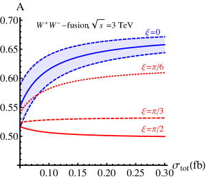
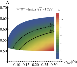
Figure 5: In the left plot: we show the expected correlation between the asymmetry ${A}$ and total cross section $\sigma_{tot}$ for different $\xi\equiv\arg(c_{t})$: the blue line with $\xi=0$ means pure CP-even $Ht\bar{t}$ coupling corresponding to the CP-conserving case (together with its $\pm 1\sigma$ uncertainty) while the three red lines with $\xi=\pi/6,\pi/3,\pi/2$ correspond to CP-violation cases. In the right plot: we show the standard deviation away from the CP-conserving case (denoted as $s_{0}=|{A}-{A}^{+}|/\sigma_{A^{+}}$, meaning the discovery potential for CP-violation) in the ${A}-\sigma_{\textrm{tot}}$ plane, together with the $3\sigma$ (dashed black line) and $5\sigma$ (solid black line) evidence and discovery boundaries, respectively.

If $\sigma_{\textrm{tot}}\gtrsim 0.08~{}\textrm{fb}$ (corresponding to $\kappa\gtrsim 0.009$ or $c_{V}\gtrsim 0.1$ if $|c_{t}|\simeq 1$), a pure CP-odd $Ht\bar{t}$ coupling is expected to be evidenced at the $3\sigma$ level; while $\sigma_{\textrm{tot}}\gtrsim 0.11~{}\textrm{fb}$ (corresponding to $\kappa\gtrsim 0.017$ or $c_{V}\gtrsim 0.14$ if $|c_{t}|\simeq 1$), a pure CP-odd $Ht\bar{t}$ coupling is expected to be discovered at $5\sigma$ level. For the largest allowed $c_{V}\simeq 0.3$ (corresponding to $\kappa\simeq 0.06$ or $\sigma_{\textrm{tot}}\simeq 0.3~{}\textrm{fb}$ if $|c_{t}|\simeq 1$), a pure CP-odd $Ht\bar{t}$ coupling corresponding to $\xi=\pi/2$ is expected to be discovered at the $11.5\sigma$ level, while the $3(5)\sigma$ evidence (discovery) boundary corresponds to $\xi\simeq 0.15\pi(0.21\pi)$.

III Implication for the 2HDM with CP-violation

III.1 Model Set-up

We choose the 2HDM with CP-violation Branco:2011iw as a test model in this section. Mainly following the conventions in Cheung:2020ugr ; Arhrib:2010ju , the Lagrangian in the scalar sector is

$$\mathcal{L}\supset\mathop{\sum}_{i=1,2}\,\left(D_{\mu}\phi_{i}\right)^{{\dagger}}\,\left(D^{\mu}\phi_{i}\right)-V\left(\phi_{1},\phi_{2}\right),$$ (15)

where $\phi_{1}=\left(\varphi_{1}^{+},\frac{1}{\sqrt{2}}(v_{1}+\eta_{1}+\textrm{i}\chi_{1})\right)^{T}$ and $\phi_{2}=\left(\varphi_{2}^{+},\frac{1}{\sqrt{2}}(v_{2}+\eta_{2}+\textrm{i}\chi_{2})\right)^{T}$ are two $\textrm{SU}(2)$ doublets. The Vacuum Expected Values (VEVs) $v_{1,2}$ satisfy the relation $v=\sqrt{|v_{1}|^{2}+|v_{2}|^{2}}=246~{}\textrm{GeV}$. We also define $t_{\beta}\equiv|v_{2}/v_{1}|$ as usual. The scalar potential is given by

$$V\left(\phi_{1},\phi_{2}\right) = -\frac{1}{2}\left[m_{1}^{2}\phi_{1}^{{\dagger}}\phi_{1}+m_{2}^{2}\phi_{2}^{{\dagger}}\phi_{2}+\left(m^{2}_{12}\phi_{1}^{{\dagger}}\phi_{2}+\textrm{H.c.}\right)\right]+\frac{1}{2}\left[\lambda_{1}\left(\phi_{1}^{{\dagger}}\phi_{1}\right)^{2}+\lambda_{2}\left(\phi_{2}^{{\dagger}}\phi_{2}\right)^{2}\right]$$ (16)

$$+\lambda_{3}\left(\phi_{1}^{{\dagger}}\phi_{1}\right)\left(\phi_{2}^{{\dagger}}\phi_{2}\right)+\lambda_{4}\left(\phi_{1}^{{\dagger}}\phi_{2}\right)\left(\phi_{2}^{{\dagger}}\phi_{1}\right)+\left[\frac{\lambda_{5}}{2}\left(\phi_{1}^{{\dagger}}\phi_{2}\right)^{2}+\textrm{H.c.}\right],$$

where we assumed a softly broken $Z_{2}$ symmetry to avoid the possible tree-level Flavour Changing Neutral Current (FCNC) interactions. Here, $m_{12}^{2}$, $\lambda_{5}$, and $v_{2}/v_{1}$ can be complex parameters and we can always perform a field rotation to make at least one of them real. We choose $v_{2}/v_{1}$ to be real and thus the vacuum conditions lead us to the relation Cheung:2020ugr ; Arhrib:2010ju

$$\textrm{Im}\left(m^{2}_{12}\right)=v_{1}v_{2}\textrm{Im}\left(\lambda_{5}\right).$$ (17)

If both sides in the equation above are non-zero, there will be CP-violation in the scalar sector. The Goldstone modes $G^{+}$ and $G^{0}$ can be recovered through a diagonalization procedure as

$$\left(\begin{array}[]{c}G^{+}\\ H^{+}\end{array}\right)=\left(\begin{array}[]{cc}c_{\beta}&s_{\beta}\\ -s_{\beta}&c_{\beta}\end{array}\right)\left(\begin{array}[]{c}\varphi_{1}^{+}\\ \varphi_{2}^{+}\end{array}\right),\quad\textrm{and}\quad\left(\begin{array}[]{c}G^{0}\\ A^{0}\end{array}\right)=\left(\begin{array}[]{cc}c_{\beta}&s_{\beta}\\ -s_{\beta}&c_{\beta}\end{array}\right)\left(\begin{array}[]{c}\chi_{1}\\ \chi_{2}\end{array}\right).$$ (18)

If there is no CP-violation, $A^{0}$ should be a pure pseudoscalar while, in the CP-violation scenario, $A^{0}$ must further mix with $\eta_{1,2}$ to obtain the neutral mass eigenstates as

$$\left(\begin{array}[]{c}H_{1}\\ H_{2}\\ H_{3}\end{array}\right)=R\left(\begin{array}[]{c}\eta_{1}\\ \eta_{2}\\ A^{0}\end{array}\right).$$ (19)

The mixing matrix $R$ is parameterized following the convention in Cheung:2020ugr as

$$R=\left(\begin{array}[]{ccc}1&&\\ &c_{\alpha_{3}}&s_{\alpha_{3}}\\ &-s_{\alpha_{3}}&c_{\alpha_{3}}\end{array}\right)\left(\begin{array}[]{ccc}c_{\alpha_{2}}&&s_{\alpha_{2}}\\ &1&\\ -s_{\alpha_{2}}&&c_{\alpha_{2}}\end{array}\right)\left(\begin{array}[]{ccc}c_{\beta+\alpha_{1}}&s_{\beta+\alpha_{1}}&\\ -s_{\beta+\alpha_{1}}&c_{\beta+\alpha_{1}}&\\ &&1\end{array}\right).$$ (20)

With this convention, if $\alpha_{1,2}\rightarrow 0$, $H_{1}$ becomes the SM Higgs boson. Here, $\alpha_{2}$ is an important parameter because it measures the CP-violation mixing corresponding to the SM-like Higgs boson $H_{1}$. In the Yukawa sector, a fermion bilinear can couple to only one scalar doublet due to the $Z_{2}$ symmetry. Denoting $Q_{L}\equiv(u,d)_{L}^{T}$ and $L_{L}\equiv(\nu,\ell)_{L}^{T}$, we always assume that $\bar{Q}_{L}u_{R}$ couples to $\phi_{2}$, and thus the four types of Yukawa interactions are

$$\mathcal{L}\supset\left\{\begin{array}[]{cl}-Y_{U}\bar{Q}_{L}\tilde{\phi}_{2}U_{R}-Y_{D}\bar{Q}_{L}\phi_{2}D_{R}-Y_{\ell}\bar{L}_{L}\phi_{2}\ell_{R}+\textrm{H.c.},&~{}(\textrm{Type I}),\\ -Y_{U}\bar{Q}_{L}\tilde{\phi}_{2}U_{R}-Y_{D}\bar{Q}_{L}\phi_{1}D_{R}-Y_{\ell}\bar{L}_{L}\phi_{1}\ell_{R}+\textrm{H.c.},&~{}(\textrm{Type II}),\\ -Y_{U}\bar{Q}_{L}\tilde{\phi}_{2}U_{R}-Y_{D}\bar{Q}_{L}\phi_{2}D_{R}-Y_{\ell}\bar{L}_{L}\phi_{1}\ell_{R}+\textrm{H.c.},&~{}(\textrm{Type III}),\\ -Y_{U}\bar{Q}_{L}\tilde{\phi}_{2}U_{R}-Y_{D}\bar{Q}_{L}\phi_{1}D_{R}-Y_{\ell}\bar{L}_{L}\phi_{2}\ell_{R}+\textrm{H.c.},&~{}(\textrm{Type IV}).\end{array}\right.$$ (21)

Following our analysis in Cheung:2020ugr , the Type I and IV models are facing very stringent electron EDM constraints and thus the CP-violation mixings are limited to $\mathcal{O}\left(10^{-3}\right)$. However, in Type II and III models, a possible cancellation between different contributions to the electron EDM leads to a much weaker constraint on the CP-violation mixing $\alpha_{2}$ Inoue:2014nva ; Mao:2014oya ; Bian:2014zka ; Fontes:2015mea ; Mao:2016jor ; Bian:2016awe ; Bian:2016zba ; Egana-Ugrinovic:2018fpy ; Fuyuto:2019svr ; Cheung:2020ugr ; Kanemura:2020ibp ; Altmannshofer:2020shb ; Low:2020iua . As shown in Cheung:2020ugr , in the Type II model $|\alpha_{2}|\lesssim 0.1$ mainly due to the neutron EDM constraint while in the Type III model $|\alpha_{2}|\lesssim 0.3$ mainly due to the global-fit on LHC Higgs data. The cancellation appears around $t_{\beta}\simeq 1$, depending weakly on $m_{2,3}$ and $\alpha_{2}$. Thus, we choose the Type III model as an example. We consider the case for which $H_{2,3}$ have a large mass splitting and $H=H_{2}$ is dominated by the pseudoscalar component, thus $\alpha_{3}\sim\pi/2$ and we have the relation

$$t_{\alpha_{3}}=\frac{\left(m_{3}^{2}-m^{2}_{2}\right)+\sqrt{\left(m^{2}_{3}-m^{2}_{2}\right)^{2}s^{2}_{2\beta+\alpha_{1}}-4\left(m^{2}_{3}-m_{1}^{2}\right)\left(m^{2}_{2}-m^{2}_{1}\right)s^{2}_{\alpha_{2}}c^{2}_{2\beta+\alpha_{1}}}}{2\left(m_{2}^{2}-m^{2}_{1}\right)s_{\alpha_{2}}c_{2\beta+\alpha_{1}}}.$$ (22)

In the Type III 2HDM, when $\alpha_{1}\simeq 0$, $\alpha_{3}\simeq\pi/2$ and $t_{\beta}\simeq 1$, the coefficients in Eq. 3 are reduced to

$$c_{V}\simeq-s_{\alpha_{2}},\quad\quad\textrm{and}\quad\quad c_{t}\simeq-s_{\alpha_{2}}-\textrm{i}c_{\alpha_{2}}=-\textrm{e}^{\textrm{i}\left(\pi/2-\alpha_{2}\right)}.$$ (23)

Thus $\alpha_{2}$ is a key parameter measuring CP-violation in the (pseudo)scalar sector.

III.2 Implications of CP-violation in the 2HDM

If we choose a scenario with the aforementioned cancellations in the electron EDM which allows larger CP-violation angle $\alpha_{2}$, we have the expected correlation between the asymmetry ${A}$ and the total cross section $\sigma_{\textrm{tot}}$, as discussed in Sec. II.3. Both ${A}$ and $\sigma_{\textrm{tot}}$ depends only on the parameter $\alpha_{2}$ for a given $m_{H}$ (and hence the electron EDM cancellation condition will fix $t_{\beta}\simeq 1$). In this scenario, the $Ht\bar{t}$ coupling is dominated by the CP-odd component and thus the expected asymmetry ${A}$ should be close to the case with pure CP-odd $Ht\bar{t}$ coupling. The $H\rightarrow Zh$ decay channel is negligible here.

In this section, we choose the $W^{+}W^{-}$-fusion channel, at CLIC with $\sqrt{s}=3~{}\textrm{TeV}$ and $10~{}\textrm{ab}^{-1}$ luminosity, as above. In the left plot of Fig. 6, we show the predicted asymmetry ${A}$ depending on the total cross section $\sigma_{\textrm{tot}}$ in this scenario of a 2HDM with $\pm 1\sigma,\pm 2\sigma,\pm 3\sigma$ uncertainties, together with the prediction from the CP-conserving case for comparison. In the right plot of Fig. 6, we show the discovery potential of CP-violation depending on the total cross section $\sigma_{\textrm{tot}}$ if an asymmetry ${A}$ equalling the 2HDM prediction is observed.

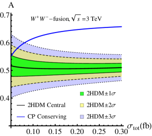
Figure 6: In the left plot: we show the predicted asymmetry ${A}$ versus the total cross section $\sigma_{\textrm{tot}}$ in the chosen 2HDM with $\pm 1\sigma$ (green), $\pm 2\sigma$ (yellow) and $\pm 3\sigma$ (blue) uncertainties. The thick black line shows the central value of the 2HDM prediction. We also show the CP-conserving prediction as the thick blue line as a comparison. In the right plot: we show the discovery potential of CP-violation versus the total cross section $\sigma_{\textrm{tot}}$ if an asymmetry ${A}$ equal to the 2HDM prediction is observed.

For the left plot, if an observed $(\sigma_{\textrm{tot}},{A})$ point is located outside the yellow (blue) boundaries, it will mean that the 2HDM scenario we discuss here is excluded at $95\%(99.7\%)$ Confidence Level (C.L.) and thus this 2HDM scenario is disfavored. And, if an asymmetry ${A}$ equal to the prediction by this 2HDM scenario is observed, meaning this 2HDM scenario is favored, we show the discovery potential of CP-violation in the right plot. We can discover CP-violation at $3(5)\sigma$ level if $\sigma_{\textrm{tot}}\gtrsim 0.08(0.11)~{}\textrm{fb}$, corresponding to $|\alpha_{2}|\gtrsim 0.096(0.14)$. Finally, for the largest allowed $|\alpha_{2}|\simeq 0.3$, corresponding to $\sigma_{\textrm{tot}}\simeq 0.3~{}\textrm{fb}$, we can discover CP-violation at the $10.7\sigma$ level.

IV Conclusions and Discussion

In this paper, we propose a novel method to test CP-violation in a (pseudo)scalar sector characterized by a heavy scalar boson $H$ with couplings to the heavy gauge bosons and a complex coupling to the top quark. We have studied the physics potential of an electron-positron collider at $\sqrt{s}=1.5$ and $3$ TeV, such as CLIC. At such high energies, the production of a heavy scalar boson is dominated by $W^{+}W^{-}$- and $ZZ$-fusion. We choose the process in which the heavy scalar $H$ is produced through VBF channel, and decays to $t\bar{t}$ pair. In our method, the CP-even component of $H$ is confirmed through the $HVV$ coupling, while the CP-odd component of $H$ should be confirmed through the CP-odd $Ht\bar{t}$ coupling. The CP nature of $Ht\bar{t}$ coupling is tested through the spin correlation between $t$ and $\bar{t}$, which is sensitive to the distribution of the azimuthal angle between the leptons decaying from $t$ and $\bar{t}$ quarks.

In our study, we found that the $ZZ$-fusion channel suffers from the SM background and cannot provide large enough significance to see the effect of CP-violation even under the most favorable scenario of CP-violation at $\sqrt{s}=1.5$ or 3 TeV. In contrast, the $W^{+}W^{-}$-fusion channel provides a reasonable separation of pure CP-even and CP-odd $Ht\bar{t}$ coupling at $\sqrt{s}=1.5$ TeV and the significant difference (more than $5\sigma$) between the CP-even and CP-odd $Ht\bar{t}$ coupling can be seen at $\sqrt{s}=3$ TeV CLIC with $10~{}\textrm{ab}^{-1}$ luminosity, under a favorable scenario of CP-violation. The physics potential is summarized in Fig. 5, in which one can see that a pure CP-odd $Ht\bar{t}$ coupling can be discovered at $5\sigma$ level for $\sigma_{\rm tot}\simeq 0.11$ fb (corresponding to $c_{V}\simeq 0.14$ if assuming $|c_{t}|=1$), and it can be stretched to $11.5\sigma$ for $\sigma_{\rm tot}\simeq 0.3$ fb (corresponding to the largest allowed $c_{V}\simeq 0.3$ if assuming $|c_{t}|=1$).

Implications for the 2HDM with CP-violation in the Higgs sector were also studied. Type III model affords a fairly large CP-violating angle $\alpha_{2}$, such that this scenario can be analyzed similarly to what we did for the model-independent approach. The results are summarized in Fig. 6. Eventually, we showed that at $\sqrt{s}=3$ TeV CLIC with $10~{}\textrm{ab}^{-1}$ luminosity, the 2HDM Type III with a favorable CP-violating set-up can be discovered at $5\sigma$ level when $\sigma_{\rm tot}\simeq 0.11$ fb (corresponding to $|\alpha_{2}|\simeq 0.14$), and it can be stretched to $10.7\sigma$ when $\sigma_{\rm tot}\simeq 0.3$ fb (corresponding to the largest allowed $|\alpha_{2}|\simeq 0.3$).

In short, an electron-positron collider operating in the multi-TeV energy range, such as CLIC, is a useful apparatus to study CP-violation effects in the (pseudo)scalar Higgs sector by using VBF production (through the charged current channel) of a heavy Higgs state decaying into a $t\bar{t}$ pair, in turn yielding two (prompt) leptons. We have come to this conclusion by performing a sophisticated Monte Carlo (MC) analysis, albeit limited to the parton level, however, we are confident that our results can be replicated at the full detector level, given that they are driven by inclusive and exclusive observables solely exploiting electron and muon kinematics.

Acknowledgements

We thank Adil Jueid for helpful discussions and collaboration at the beginning of this project. We also thank Kechen Wang for helpful discussion about statistics and collider phenomenology. Y.N.M. thanks the Center for Future High Energy Physics (Institute of High Energy Physics, Chinese Academy of Sciences, Beijing) for hospitality when part of this work was done. Y.N.M. is partially supported by the National Natural Science Foundation of China (Grant No. 12205227) and the Fundamental Research Funds for the Central Universities (WUT: 2022IVA052). S.M. is supported in part through the NExT Institute and the STFC Consolidated Grant No. ST/L000296/1. K.C. is supported in part by the National Science and Technology Council of Taiwan under the grant number MoST 110-2112-M-007-017-MY3. R.Z. is partially supported by the National Natural Science Foundation of China (Grant No. 12075257), the funding from the Institute of High Energy Physics, Chinese Academy of Sciences (Y6515580U1), and the funding from Chinese Academy of Sciences (Y8291120K2).

References

- (1) J. H. Christenson, J. W. Cronin, V. L. Fitch and R. Turlay, Evidence for the Decay of the Meson, Phys. Rev. Lett. 13 (1964) 138–140.
- (2) LHCb collaboration, R. Aaij et al., Observation of CP Violation in Charm Decays, Phys. Rev. Lett. 122 (2019) 211803, [1903.08726].
- (3) Particle Data Group collaboration, P. Zyla et al., Review of Particle Physics, PTEP 2020 (2020) 083C01.
- (4) Particle Data Group collaboration, R. L. Workman et al., Review of Particle Physics, PTEP 2022 (2022) 083C01.
- (5) S. Khalil and S. Moretti, Standard Model Phenomenology. CRC Press, 6, 2022.
- (6) M. Kobayashi and T. Maskawa, CP Violation in the Renormalizable Theory of Weak Interaction, Prog. Theor. Phys. 49 (1973) 652–657.
- (7) A. G. Cohen, D. B. Kaplan and A. E. Nelson, Spontaneous baryogenesis at the weak phase transition, Phys. Lett. B 263 (1991) 86–92.
- (8) A. G. Cohen, D. B. Kaplan and A. E. Nelson, Progress in electroweak baryogenesis, Ann. Rev. Nucl. Part. Sci. 43 (1993) 27–70, [hep-ph/9302210].
- (9) D. E. Morrissey and M. J. Ramsey-Musolf, Electroweak baryogenesis, New J. Phys. 14 (2012) 125003, [1206.2942].
- (10) ACME collaboration, V. Andreev et al., Improved limit on the electric dipole moment of the electron, Nature 562 (2018) 355–360.
- (11) W. B. Cairncross, D. N. Gresh, M. Grau, K. C. Cossel, T. S. Roussy, Y. Ni et al., Precision Measurement of the Electron’s Electric Dipole Moment Using Trapped Molecular Ions, Phys. Rev. Lett. 119 (2017) 153001, [1704.07928].
- (12) nEDM collaboration, C. Abel et al., Measurement of the permanent electric dipole moment of the neutron, Phys. Rev. Lett. 124 (2020) 081803, [2001.11966].
- (13) J. Engel, M. J. Ramsey-Musolf and U. van Kolck, Electric Dipole Moments of Nucleons, Nuclei, and Atoms: The Standard Model and Beyond, Prog. Part. Nucl. Phys. 71 (2013) 21–74, [1303.2371].
- (14) N. Yamanaka, B. K. Sahoo, N. Yoshinaga, T. Sato, K. Asahi and B. P. Das, Probing exotic phenomena at the interface of nuclear and particle physics with the electric dipole moments of diamagnetic atoms: A unique window to hadronic and semi-leptonic CP violation, Eur. Phys. J. A 53 (2017) 54, [1703.01570].
- (15) M. S. Safronova, D. Budker, D. DeMille, D. F. J. Kimball, A. Derevianko and C. W. Clark, Search for New Physics with Atoms and Molecules, Rev. Mod. Phys. 90 (2018) 025008, [1710.01833].
- (16) T. Chupp, P. Fierlinger, M. Ramsey-Musolf and J. Singh, Electric dipole moments of atoms, molecules, nuclei, and particles, Rev. Mod. Phys. 91 (2019) 015001, [1710.02504].
- (17) M. Pospelov and A. Ritz, Electric dipole moments as probes of new physics, Annals Phys. 318 (2005) 119–169, [hep-ph/0504231].
- (18) Y. Yamaguchi and N. Yamanaka, Large long-distance contributions to the electric dipole moments of charged leptons in the standard model, Phys. Rev. Lett. 125 (2020) 241802, [2003.08195].
- (19) Y. Yamaguchi and N. Yamanaka, Quark level and hadronic contributions to the electric dipole moment of charged leptons in the standard model, Phys. Rev. D 103 (2021) 013001, [2006.00281].
- (20) L. Bento, G. C. Branco and P. A. Parada, A Minimal model with natural suppression of strong CP violation, Phys. Lett. B 267 (1991) 95–99.
- (21) T. D. Lee, A Theory of Spontaneous T Violation, Phys. Rev. D8 (1973) 1226–1239.
- (22) T. D. Lee, CP Nonconservation and Spontaneous Symmetry Breaking, Phys. Rept. 9 (1974) 143–177.
- (23) G. C. Branco, P. M. Ferreira, L. Lavoura, M. N. Rebelo, M. Sher and J. P. Silva, Theory and phenomenology of two-Higgs-doublet models, Phys. Rept. 516 (2012) 1–102, [1106.0034].
- (24) S. Weinberg, Gauge Theory of CP Violation, Phys. Rev. Lett. 37 (1976) 657.
- (25) K. Cheung, A. Jueid, Y.-n. Mao and S. Moretti, Two-Higgs-doublet model with soft CP violation confronting electric dipole moments and colliders, Phys. Rev. D 102 (2020) 075029, [2003.04178].
- (26) A. W. El Kaffas, W. Khater, O. M. Ogreid and P. Osland, Consistency of the two Higgs doublet model and CP violation in top production at the LHC, Nucl. Phys. B 775 (2007) 45–77, [hep-ph/0605142].
- (27) S. Berge, W. Bernreuther and J. Ziethe, Determining the CP parity of Higgs bosons at the LHC in their tau decay channels, Phys. Rev. Lett. 100 (2008) 171605, [0801.2297].
- (28) J. Shu and Y. Zhang, Impact of a CP Violating Higgs Sector: From LHC to Baryogenesis, Phys. Rev. Lett. 111 (2013) 091801, [1304.0773].
- (29) Y.-n. Mao and S.-h. Zhu, Lightness of Higgs boson and spontaneous CP violation in the Lee model, Phys. Rev. D 90 (2014) 115024, [1409.6844].
- (30) C.-Y. Chen, S. Dawson and Y. Zhang, Complementarity of LHC and EDMs for Exploring Higgs CP Violation, JHEP 06 (2015) 056, [1503.01114].
- (31) V. Keus, S. F. King, S. Moretti and K. Yagyu, CP Violating Two-Higgs-Doublet Model: Constraints and LHC Predictions, JHEP 04 (2016) 048, [1510.04028].
- (32) D. Fontes, J. C. Romo, R. Santos and J. P. Silva, Large pseudoscalar Yukawa couplings in the complex 2HDM, JHEP 06 (2015) 060, [1502.01720].
- (33) L. Bian and N. Chen, Higgs pair productions in the CP-violating two-Higgs-doublet model, JHEP 09 (2016) 069, [1607.02703].
- (34) Y.-n. Mao and S.-h. Zhu, Lightness of a Higgs Boson and Spontaneous CP-violation in the Lee Model: An Alternative Scenario, Phys. Rev. D 94 (2016) 055008, [1602.00209].
- (35) K. Hagiwara, K. Ma and S. Mori, Probing CP violation in at the LHC, Phys. Rev. Lett. 118 (2017) 171802, [1609.00943].
- (36) C.-Y. Chen, H.-L. Li and M. Ramsey-Musolf, CP-Violation in the Two Higgs Doublet Model: from the LHC to EDMs, Phys. Rev. D 97 (2018) 015020, [1708.00435].
- (37) Q.-H. Cao, K.-P. Xie, H. Zhang and R. Zhang, A New Observable for Measuring CP Property of Top-Higgs Interaction, Chin. Phys. C 45 (2021) 023117, [2008.13442].
- (38) D. Azevedo, R. Capucha, E. Gouveia, A. Onofre and R. Santos, Light Higgs searches in production at the LHC, JHEP 04 (2021) 077, [2012.10730].
- (39) D. Azevedo, R. Capucha, A. Onofre and R. Santos, Scalar mass dependence of angular variables in production, JHEP 06 (2020) 155, [2003.09043].
- (40) S. Antusch, O. Fischer, A. Hammad and C. Scherb, Testing CP Properties of Extra Higgs States at the HL-LHC, JHEP 03 (2021) 200, [2011.10388].
- (41) S. Kanemura, M. Kubota and K. Yagyu, Testing aligned CP-violating Higgs sector at future lepton colliders, JHEP 04 (2021) 144, [2101.03702].
- (42) I. Low, N. R. Shah and X.-P. Wang, Higgs alignment and novel CP-violating observables in two-Higgs-doublet models, Phys. Rev. D 105 (2022) 035009, [2012.00773].
- (43) ATLAS collaboration, G. Aad et al., Observation of a new particle in the search for the Standard Model Higgs boson with the ATLAS detector at the LHC, Phys. Lett. B 716 (2012) 1–29, [1207.7214].
- (44) CMS collaboration, S. Chatrchyan et al., Observation of a New Boson at a Mass of 125 GeV with the CMS Experiment at the LHC, Phys. Lett. B 716 (2012) 30–61, [1207.7235].
- (45) ATLAS, CMS collaboration, G. Aad et al., Combined Measurement of the Higgs Boson Mass in Collisions at and 8 TeV with the ATLAS and CMS Experiments, Phys. Rev. Lett. 114 (2015) 191803, [1503.07589].
- (46) C. R. Schmidt and M. E. Peskin, A Probe of CP violation in top quark pair production at hadron supercolliders, Phys. Rev. Lett. 69 (1992) 410–413.
- (47) G. Mahlon and S. J. Parke, Angular correlations in top quark pair production and decay at hadron colliders, Phys. Rev. D53 (1996) 4886–4896, [hep-ph/9512264].
- (48) E. Asakawa and K. Hagiwara, Probing the CP nature of the Higgs bosons by t anti-t production at photon linear colliders, Eur. Phys. J. C 31 (2003) 351–364, [hep-ph/0305323].
- (49) P. S. Bhupal Dev, A. Djouadi, R. M. Godbole, M. M. Muhlleitner and S. D. Rindani, Determining the CP properties of the Higgs boson, Phys. Rev. Lett. 100 (2008) 051801, [0707.2878].
- (50) X.-G. He, G.-N. Li and Y.-J. Zheng, Probing Higgs boson Properties with at the LHC and the 100 TeV collider, Int. J. Mod. Phys. A 30 (2015) 1550156, [1501.00012].
- (51) F. Boudjema, R. M. Godbole, D. Guadagnoli and K. A. Mohan, Lab-frame observables for probing the top-Higgs interaction, Phys. Rev. D92 (2015) 015019, [1501.03157].
- (52) M. R. Buckley and D. Goncalves, Boosting the Direct CP Measurement of the Higgs-Top Coupling, Phys. Rev. Lett. 116 (2016) 091801, [1507.07926].
- (53) S. Amor Dos Santos et al., Probing the CP nature of the Higgs coupling in events at the LHC, Phys. Rev. D96 (2017) 013004, [1704.03565].
- (54) D. Azevedo, A. Onofre, F. Filthaut and R. Goncalo, CP tests of Higgs couplings in semileptonic events at the LHC, Phys. Rev. D 98 (2018) 033004, [1711.05292].
- (55) W. Bernreuther, L. Chen, I. Garca, M. Perell, R. Poeschl, F. Richard et al., CP-violating top quark couplings at future linear colliders, Eur. Phys. J. C78 (2018) 155, [1710.06737].
- (56) K. Hagiwara, H. Yokoya and Y.-J. Zheng, Probing the CP properties of top Yukawa coupling at an collider, JHEP 02 (2018) 180, [1712.09953].
- (57) K. Ma, Enhancing Measurement of the Yukawa Interactions of Top-Quark at Collider, Phys. Lett. B 797 (2019) 134928, [1809.07127].
- (58) M. Cepeda et al., Report from Working Group 2: Higgs Physics at the HL-LHC and HE-LHC, CERN Yellow Rep. Monogr. 7 (2019) 221–584, [1902.00134].
- (59) D. A. Faroughy, J. F. Kamenik, N. Konik and A. Smolkovi, Probing the nature of the top quark Yukawa at hadron colliders, JHEP 02 (2020) 085, [1909.00007].
- (60) K. Desch, A. Imhof, Z. Was and M. Worek, Probing the CP nature of the Higgs boson at linear colliders with tau spin correlations: The Case of mixed scalar - pseudoscalar couplings, Phys. Lett. B 579 (2004) 157–164, [hep-ph/0307331].
- (61) R. Harnik, A. Martin, T. Okui, R. Primulando and F. Yu, Measuring CP Violation in at Colliders, Phys. Rev. D88 (2013) 076009, [1308.1094].
- (62) S. Berge, W. Bernreuther and H. Spiesberger, Higgs CP properties using the decay modes at the ILC, Phys. Lett. B 727 (2013) 488–495, [1308.2674].
- (63) S. Berge, W. Bernreuther and S. Kirchner, Determination of the Higgs CP-mixing angle in the tau decay channels at the LHC including the Drell–Yan background, Eur. Phys. J. C 74 (2014) 3164, [1408.0798].
- (64) S. Berge, W. Bernreuther and S. Kirchner, Prospects of constraining the Higgs boson’s CP nature in the tau decay channel at the LHC, Phys. Rev. D92 (2015) 096012, [1510.03850].
- (65) A. Askew, P. Jaiswal, T. Okui, H. B. Prosper and N. Sato, Prospect for measuring the CP phase in the coupling at the LHC, Phys. Rev. D 91 (2015) 075014, [1501.03156].
- (66) R. Jzefowicz, E. Richter-Was and Z. Was, Potential for optimizing the Higgs boson CP measurement in H decays at the LHC including machine learning techniques, Phys. Rev. D 94 (2016) 093001, [1608.02609].
- (67) G. Li, Y.-n. Mao, C. Zhang and S.-h. Zhu, Testing CP violation in the scalar sector at future colliders, Phys. Rev. D95 (2017) 035015, [1611.08518].
- (68) Y.-n. Mao, Spontaneous CP-violation in the Simplest Little Higgs Model and its Future Collider Tests: the Scalar Sector, Phys. Rev. D 97 (2018) 075031, [1703.10123].
- (69) Y.-n. Mao, Spontaneous CP-violation in the Simplest Little Higgs Model, PoS ICHEP2018 (2019) 003, [1810.03854].
- (70) S. De Curtis, S. Moretti, R. Nagai and K. Yagyu, CP-Violation in a composite 2-Higgs doublet model, JHEP 10 (2021) 040, [2107.08201].
- (71) L. Linssen, A. Miyamoto, M. Stanitzki and H. Weerts, Physics and Detectors at CLIC: CLIC Conceptual Design Report. CERN Yellow Reports: Monographs. CERN, Geneva, 2012, 10.5170/CERN-2012-003.
- (72) P. Lebrun, L. Linssen, A. Lucaci-Timoce, D. Schulte, F. Simon, S. Stapnes et al., The CLIC programme: Towards a staged linear collider exploring the terascale: CLIC conceptual design report. CERN Yellow Reports: Monographs. CERN, Geneva, 2012, 10.5170/CERN-2012-005.
- (73) H. Abramowicz et al., Higgs physics at the CLIC electron–positron linear collider, Eur. Phys. J. C 77 (2017) 475, [1608.07538].
- (74) CLIC accelerator collaboration, M. Aicheler, P. N. Burrows, N. Catalan Lasheras, R. Corsini, M. Draper, J. Osborne et al., eds., The Compact Linear Collider (CLIC) - Project Implementation Plan, vol. 4/2018. 12, 2018, 10.23731/CYRM-2018-004.
- (75) CLIC collaboration, J. de Blas et al., The CLIC Potential for New Physics, vol. 3/2018. 12, 2018, 10.23731/CYRM-2018-003.
- (76) CLICdp, CLIC collaboration, T. K. Charles et al., The Compact Linear Collider (CLIC) - 2018 Summary Report, vol. 2/2018. 12, 2018, 10.23731/CYRM-2018-002.
- (77) O. Brunner et al., The CLIC project, 2203.09186.
- (78) G. Mahlon and S. J. Parke, Spin Correlation Effects in Top Quark Pair Production at the LHC, Phys. Rev. D81 (2010) 074024, [1001.3422].
- (79) ATLAS collaboration, G. Aad et al., Observation of spin correlation in events from pp collisions at sqrt(s) = 7 TeV using the ATLAS detector, Phys. Rev. Lett. 108 (2012) 212001, [1203.4081].
- (80) M. Baumgart and B. Tweedie, A New Twist on Top Quark Spin Correlations, JHEP 03 (2013) 117, [1212.4888].
- (81) J. Ellis, D. S. Hwang, K. Sakurai and M. Takeuchi, Disentangling Higgs-Top Couplings in Associated Production, JHEP 04 (2014) 004, [1312.5736].
- (82) N. Mileo, K. Kiers, A. Szynkman, D. Crane and E. Gegner, Pseudoscalar top-Higgs coupling: exploration of CP-odd observables to resolve the sign ambiguity, JHEP 07 (2016) 056, [1603.03632].
- (83) J. A. Aguilar-Saavedra, Dilepton azimuthal correlations in production, JHEP 09 (2018) 116, [1806.07438].
- (84) ATLAS collaboration, G. Aad et al., Search for heavy resonances decaying into a pair of Z bosons in the and final states using 139 of proton–proton collisions at TeV with the ATLAS detector, Eur. Phys. J. C 81 (2021) 332, [2009.14791].
- (85) J. Alwall, R. Frederix, S. Frixione, V. Hirschi, F. Maltoni, O. Mattelaer et al., The automated computation of tree-level and next-to-leading order differential cross sections, and their matching to parton shower simulations, JHEP 07 (2014) 079, [1405.0301].
- (86) S. Frixione, O. Mattelaer, M. Zaro and X. Zhao, Lepton collisions in MadGraph5_aMC@NLO, 2108.10261.
- (87) A. Arhrib, E. Christova, H. Eberl and E. Ginina, CP violation in charged Higgs production and decays in the Complex Two Higgs Doublet Model, JHEP 04 (2011) 089, [1011.6560].
- (88) S. Inoue, M. J. Ramsey-Musolf and Y. Zhang, CP-violating phenomenology of flavor conserving two Higgs doublet models, Phys. Rev. D 89 (2014) 115023, [1403.4257].
- (89) L. Bian, T. Liu and J. Shu, Cancellations Between Two-Loop Contributions to the Electron Electric Dipole Moment with a CP-Violating Higgs Sector, Phys. Rev. Lett. 115 (2015) 021801, [1411.6695].
- (90) L. Bian and N. Chen, Cancellation mechanism in the predictions of electric dipole moments, Phys. Rev. D 95 (2017) 115029, [1608.07975].
- (91) D. Egana-Ugrinovic and S. Thomas, Higgs Boson Contributions to the Electron Electric Dipole Moment, 1810.08631.
- (92) K. Fuyuto, W.-S. Hou and E. Senaha, Cancellation mechanism for the electron electric dipole moment connected with the baryon asymmetry of the Universe, Phys. Rev. D 101 (2020) 011901, [1910.12404].
- (93) S. Kanemura, M. Kubota and K. Yagyu, Aligned CP-violating Higgs sector canceling the electric dipole moment, JHEP 08 (2020) 026, [2004.03943].
- (94) W. Altmannshofer, S. Gori, N. Hamer and H. H. Patel, Electron EDM in the complex two-Higgs doublet model, Phys. Rev. D 102 (2021) 115042, [2009.01258].