Integral equation method for the 1D steady-state Poisson-Nernst-Planck equations

Abstract

An integral equation method is presented for the 1D steady-state Poisson-Nernst-Planck equations modeling ion transport through membrane channels. The differential equations are recast as integral equations using Green’s 3rd identity yielding a fixed-point problem for the electric potential gradient and ion concentrations. The integrals are discretized by a combination of midpoint and trapezoid rules and the resulting algebraic equations are solved by Gummel iteration. Numerical tests for electroneutral and non-electroneutral systems demonstrate the method’s 2nd order accuracy and ability to resolve sharp boundary layers. The method is applied to a 1D model of the K⁺ ion channel with a fixed charge density that ensures cation selectivity. In these tests the proposed integral equation method yields potential and concentration profiles in good agreement with published results.

1 Introduction

Ion transport through membrane channels is a fundamental process in cell biology hille1978ionic ; hille2001ion . However, atomistic simulations of this process are expensive and an alternative continuum approach is based on the Poisson-Nernst-Planck (PNP) equations, where the Poisson equation for the electric potential is coupled to the Nernst-Planck equation for the ion concentrations. The continuum PNP model accounts for two effects, (1) molecular diffusion due to ion concentration gradients, and (2) ion drift in the applied and self-consistent electric fields. The PNP equations have been employed to study many aspects of ion channel selectivity liu2017incorporating , including the effect of fixed charge eisenberg_poissonnernstplanck_2007 , ion size horng2012pnp , and membrane surface charge xie2020finite .

Despite the relative efficiency in comparison with atomistic simulations, numerical solution of the PNP equations is still challenging due to several factors, (1) nonlinear coupling of the electric potential and ion concentrations, (2) the need to resolve the channel geometry, as well as boundary layers and internal layers at material interfaces, and (3) maintaining stability in convection-dominated cases wang2021stabilized . Many PNP solvers have been developed using finite-difference methods zheng_second-order_2011 ; flavell2014conservative , finite-element methods lu2007electrodiffusion ; lu_poissonnernstplanck_2010 ; xie2020finite ; xie2020effective , and finite-volume methods chainais2003convergence ; song2018electroneutral ; song2019selectivity . It is also important for numerical PNP solvers to preserve positivity of the ion concentrations and conserve mass in time-dependent simulations, and several implicit finite-difference schemes have been developed for this purpose flavell2014conservative ; hu2020fully .

The boundary element method (BEM) is another approach to solving linear elliptic boundary value problems, where the differential equation is recast as an integral equation on the domain boundary by convolution with an appropriate Green’s function steinbach2007numerical . While the BEM requires discretization of singular integrals, it has the advantage of reduced spatial dimension. Closely related to the PNP equations is the Poisson-Boltzmann (PB) equation for the electrostatic potential of a solvated protein. The BEM has been applied to solve the 3D linear PB equation on the molecular surface of a protein (see juffer1991electric ; geng2013treecode and references therein), but aside from some early work using a Green’s function to solve the PB equation for an ion channel in 1D barcilon1992ion , as far as we know this approach has not been further developed for 2D and 3D ion channel problems.

In fact there are two challenges to applying an integral equation approach to the PNP system, (1) nonlinear coupling of the electric potential and ion concentrations, and (2) the ions are distributed throughout the channel and solvent domain requiring costly volume integrals in 2D and 3D. Nonetheless we believe these obstacles can be overcome using iteration to handle the nonlinearity, and a fast summation method with adaptive quadrature for the volume integrals. As a step in that direction, the present work develops a novel integral equation method for the 1D steady-state PNP equations.

The paper is organized as follows. Section 2 introduces the 1D steady-state PNP equations. Section 3 uses Green’s 3rd identity to recast the PNP equations as a fixed-point problem involving integral operators for the potential gradient and ion concentrations. Section 4 presents the numerical implementation. Section 5 presents tests for electroneutral and non-electroneutral systems with Robin boundary conditions on the potential and no-flux boundary conditions on the ion concentrations. Section 6 presents a K⁺ ion channel simulation following gardner2004electrodiffusion and the work is summarized in Section 7.

2 PNP equations

This work focuses on the 1D steady-state PNP equations with two ion species. The electrostatic potential $\phi(x)$ satisfies the Poisson equation,

$$-\left(\epsilon\phi^{\prime}(x)\right)^{\prime}=z_{1}ec_{1}(x)+z_{2}ec_{2}(x),$$ (1)

where $\epsilon$ is the permittivity, the valence is $z_{1}=-1$ for anions and $z_{2}=1$ for cations, $e$ is the proton charge, $c_{1}(x),c_{2}(x)$ are the ion concentrations, and the domain is $[-L,L]$. This is supplemented with the Nernst–Planck equation,

$$\left[D_{i}\left(c_{i}^{\prime}(x)+\frac{z_{i}e}{k_{B}T}c_{i}(x)\phi^{\prime}(x)\right)\right]^{\prime}=0,$$ (2)

for $i=1,2$, where $D_{i},k_{B},T$ are the diffusion coefficient of ion species $i$, Boltzmann constant, and absolute temperature.

Following flavell2014conservative the PNP equations are non-dimensionalized with respect to the bulk concentration $c_{0}$ [ions/ų], channel half-length $L$ [Å], characteristic diffusion coefficient $D_{0}$ [Ų/s], characteristic potential $\phi_{0}$ [V], and water permittivity $\epsilon_{t}$ [F/Å]. The resulting non-dimensional equations are

$$-\epsilon\phi^{\prime\prime}(x)=\chi_{2}\left(z_{1}c_{1}(x)+z_{2}c_{2}(x)\right),$$ (3a)

$$\left(D_{i}\left(c_{i}^{\prime}(x)+\chi_{1}z_{i}c_{i}(x)\phi^{\prime}(x)\right)\right)^{\prime}=0,$$ (3b)

for $i=1,2$ with domain $[-1,1]$. The coefficients are

$$\chi_{1}=\frac{e\phi_{0}}{k_{B}T},\quad\chi_{2}=\frac{ec_{0}L^{2}}{\phi_{0}\epsilon_{t}},$$ (4)

where $\chi_{1}$ is the ratio of electric potential energy to thermal energy, and $\chi_{2}$ is the inverse square of the scaled Debye length. Except as otherwise noted, the non-dimensional diffusion coefficient is $D_{i}=1$.

2.1 Problem specification

The first set of examples are electroneutral and non-electroneutral systems, where the non-dimensional PNP equations (3) are solved on the interval $[-1,1]$. We consider Robin boundary conditions for the potential,

$$\phi(x)\pm\eta\phi^{\prime}(x)=\phi_{\pm},\quad x=-1,1,$$ (5)

where $\eta,\phi_{\pm}$ are constants that depend on biological modeling considerations. Note that if $\eta=0$, then (5) reduces to Dirichlet boundary conditions for the potential. The channel is assumed to be closed at both ends, hence the no-flux boundary condition is applied for the ion concentrations,

$$D_{i}\left(c_{i}^{\prime}(x)+\chi_{1}z_{i}c_{i}(x)\phi^{\prime}(x)\right)=0,\quad x=-1,1.$$ (6)

Finally, the total concentration for each ion species is a specified positive constant,

$$\int_{-1}^{1}c_{i}(x)dx=a_{i},\quad i=1,2.$$ (7)

In addition to the electroneutral and non-electroneautral systems, we also consider a K⁺ ion channel model and the problem specification in that case is given further below.

3 Integral form

This section recasts the 1D steady state PNP differential equations as a set of integral equations in the form

$$\phi^{\prime} ={\bf P}[c_{1},c_{2}],$$ (8a)

$$c_{i} ={\bf NP}[c_{i},\phi^{\prime}],\quad i=1,2,$$ (8b)

where ${\bf P},{\bf NP}$ are operators obtained by integrating the Poisson and Nernst-Planck equations while incorporating the Robin and no-flux boundary conditions and the total concentration condition. Note that (8) defines a fixed-point problem, where ${\bf P}$ maps the concentrations $c_{1},c_{2}$ into the potential gradient $\phi^{\prime}$, while ${\bf NP}$ maps the concentration $c_{i}$ and potential gradient $\phi^{\prime}$ into the concentration $c_{i}$ for $i=1,2$. The integral form of the PNP equations in (8) is solved by Gummel iteration gummel1964self for $\phi^{\prime},c_{1},c_{2}$, and once it converges, further processing yields the potential $\phi$ and the concentration gradients $c_{1}^{\prime},c_{2}^{\prime}$ needed to compute the current. Note that a fixed-point formulation and Gummel iteration was also used in the analysis of semiconductor drift-diffusion equations, although without recasting the differential equations as integral equations jerome1985consistency .

The derivation of the ${\bf P}$ and ${\bf NP}$ operators relies on Green’s 3rd identity,

$$f(x) =\Big{[}g(x,y)f^{\prime}(y)-g_{y}(x,y)f(y)\Big{]}_{y=-1}^{y=1}$$ (9)

$$-\int_{-1}^{1}g(x,y)f^{\prime\prime}(y)dy,$$

where $f(x)$ is twice continuously differentiable on $[-1,1]$ and $g(x,y)$ is the 1D free-space Laplace Green’s function,

$$g(x,y)=-\frac{1}{2}\lvert x-y\rvert.$$ (10)

Note that among the two terms on the right side of (9), the first term (or bracket term) involves the boundary values $f(\pm 1),f^{\prime}(\pm 1)$, and the second term (or volume integral term) involves $f^{\prime\prime}(x)$ over the entire interval. One can think of (9) as defining an operator, where $f(\pm 1),f^{\prime}(\pm 1),f^{\prime\prime}(x)$ are the input and $f(x)$ is the output. This point of view is taken in reformulating the PNP equations.

3.1 Derivation of P operator

Here we assume the ion concentrations $c_{1}(x),c_{2}(x)$ are given and we shall derive an integral expression for the potential gradient $\phi^{\prime}(x)$. The Poisson equation (3a) is written as

$$\phi^{\prime\prime}(x)=-\frac{\chi_{2}}{\varepsilon}\sum\limits_{i=1}^{2}z_{i}c_{i}(x),$$ (11)

and then applying (9) with $f(y)=\phi(y)$ yields an integral expression for the potential,

$$\phi(x) =\Big{[}g(x,y)\phi^{\prime}(y)-g_{y}(x,y)\phi(y)\Big{]}_{y=-1}^{y=1}$$ (12)

$$+\frac{\chi_{2}}{\epsilon}\sum_{i=1}^{2}z_{i}\int_{-1}^{1}g(x,y)c_{i}(y)dy.$$

Differentiating (12) yields an analogous expression for the potential gradient,

$$\phi^{\prime}(x) =\Big{[}g_{x}(x,y)\phi^{\prime}(y)-g_{xy}(x,y)\phi(y)\Big{]}_{y=-1}^{y=1}$$ (13)

$$+\frac{\chi_{2}}{\epsilon}\sum_{i=1}^{2}z_{i}\int_{-1}^{1}g_{x}(x,y)c_{i}(y)dy.$$

The bracket terms in (12) and (13) involve the boundary values of the potential $\phi(\pm 1)$ and potential gradient $\phi^{\prime}(\pm 1)$. The Robin boundary conditions (5) provide two equations for these four unknowns and two more equations are obtained as follows.

Integrating the Poisson equation (11) over $[-1,x]$ yields

$$\phi^{\prime}(x)-\phi^{\prime}(-1)=-\frac{\chi_{2}}{\epsilon}\int_{-1}^{x}\sum_{i=1}^{2}z_{i}c_{i}(s)ds,$$ (14)

and setting $x=1$ yields

$$\phi^{\prime}(1)-\phi^{\prime}(-1)=-\frac{\chi_{2}}{\epsilon}\sum_{i=1}^{2}z_{i}a_{i}.$$ (15)

Then integrating (14) over $[-1,1]$ yields

$$\phi(1)-\phi(-1)-2\phi^{\prime}(-1)=-\frac{\chi_{2}}{\epsilon}\sum_{i=1}^{2}z_{i}(a_{i}-b_{i}),$$ (16)

where $a_{i}$ is the total concentration of ion species $i$ defined in (7) and

$$b_{i}=\int_{-1}^{1}xc_{i}(x)dx,\quad i=1,2,$$ (17)

is the first moment of the ion concentration. By similar steps, integrating the Poisson equation (11) over $[x,1]$ yields

$$\phi(1)-\phi(-1)-2\phi^{\prime}(1)=\frac{\chi_{2}}{\epsilon}\sum_{i=1}^{2}z_{i}(a_{i}+b_{i}).$$ (18)

Then adding (16) and (18) yields

$$\phi(1)-\phi(-1)-\phi^{\prime}(1)-\phi^{\prime}(-1)=\frac{\chi_{2}}{\epsilon}\sum_{i=1}^{2}z_{i}b_{i}.$$ (19)

Combining the Robin boundary conditions (5) with (15) and (19) yields the linear system

$$\begin{pmatrix}1&\eta&0&0\\ 0&0&1&-\eta\\ 0&1&0&-1\\ 1&-1&-1&-1\\ \end{pmatrix}\begin{pmatrix}\phi(1)\\ \phi^{\prime}(1)\\ \phi(-1)\\ \phi^{\prime}(-1)\end{pmatrix}=\begin{pmatrix}\phi_{+}\\ \phi_{-}\\ \displaystyle-\frac{\chi_{2}}{\epsilon}\sum\limits_{i=1}^{2}z_{i}a_{i}\\ \displaystyle\hfill\frac{\chi_{2}}{\epsilon}\sum\limits_{i=1}^{2}z_{i}b_{i}\\ \end{pmatrix}.$$ (20)

Hence given ion concentrations $c_{1}(x),c_{2}(x)$ for $x\in[-1,1]$, the ${\bf P}$ operator in (8a) is defined by the following steps.

• compute the side right of the linear system (20) and solve for the potential boundary values $\phi(\pm 1),\phi^{\prime}(\pm 1)$

• compute the interior values of the potential gradient $\phi^{\prime}(x)$ for $x\in(-1,1)$ from (13)

These steps require computing certain integrals and the discretization schemes will be explained further below.

3.2 Derivation of NP operator

Here we assume the ion concentration $c_{i}(x)$ and potential gradient $\phi^{\prime}(x)$ are given and we shall derive an integral expression for $c_{i}(x)$. The Nernst-Planck equation (3b) is written as

$$c_{i}^{\prime\prime}(x)=-\chi_{1}z_{i}(c_{i}(x)\phi^{\prime}(x))^{\prime},$$ (21)

after cancelling the constant diffusion coefficient $D_{i}$, and then applying (9) with $f(x)=c_{i}(x)$ yields an integral expression for the ion concentration,

$$c_{i}(x) =\Big{[}g(x,y)c_{i}^{\prime}(y)-g_{y}(x,y)c_{i}(y)\Big{]}_{y=-1}^{y=1}$$ (22)

$$+\chi_{1}z_{i}\int_{-1}^{1}g(x,y)\left(c_{i}(y)\phi^{\prime}(y)\right)^{\prime}dy.$$

Differentiating (22) yields an analogous expression for the concentration gradient,

$$c_{i}^{\prime}(x) =\Big{[}g_{x}(x,y)c_{i}^{\prime}(y)-g_{xy}(x,y)c_{i}(x)\Big{]}_{y=-1}^{y=1}$$ (23)

$$+\chi_{1}z_{i}\int_{-1}^{1}g_{x}(x,y)\left(c_{i}(y)\phi^{\prime}(y)\right)^{\prime}dy.$$

The bracket terms in (22) and (23) involve the boundary values of the concentration $c_{i}(\pm 1)$ and concentration gradient $c_{i}^{\prime}(\pm 1)$. The solution procedure in this case is somewhat different than what was described above for the ${\bf P}$ operator.

From the Nernst-Planck equation (3b) and no-flux boundary conditions (6), it follows that

$$c_{i}^{\prime}(x)+\chi_{1}z_{i}c_{i}(x)\phi^{\prime}(x)=0,\quad x\in(-1,1).$$ (24)

Integrating (24) over $[-1,x]$ yields

$$c_{i}(x)-c_{i}(-1)=-\chi_{1}z_{i}\int_{-1}^{x}c_{i}(s)\phi^{\prime}(s)ds,$$ (25)

and setting $x=1$ yields

$$c_{i}(1)-c_{i}(-1)=-\chi_{1}z_{i}\int_{-1}^{1}c_{i}(s)\phi^{\prime}(s)ds.$$ (26)

Then integrating (25) over $[-1,1]$ yields

$$c_{i}(1)+c_{i}(-1)=a_{i}-\chi_{1}z_{i}\!\int_{-1}^{1}\!\!xc_{i}(x)\phi^{\prime}(x)dx.$$ (27)

Hence given the ion concentration $c_{i}(x)$ and potential gradient $\phi^{\prime}(x)$ for $x\in[-1,1]$, the ${\bf NP}$ operator in (8b) is defined by the following steps.

• compute the integrals on the right of (26)-(27) and solve for the concentration boundary values $c_{i}(\pm 1)$ on the left

• compute the concentration gradient boundary values $c_{i}^{\prime}(\pm 1)$ using $c_{i}(\pm 1)$ and the no-flux boundary conditions (6)

• compute the interior concentration $c_{i}(x)$ for $x\in(-1,1)$ from (22)

This concludes the derivation of the ${\bf P},{\bf NP}$ operators in the integral form of the PNP equations (8).

4 Numerical method

This section presents the numerical method used to solve the integral form of the PNP equations with the Robin and no-flux boundary conditions and total concentration constraint. The domain $[-1,1]$ is divided into $N$ subintervals with endpoints $x_{k},k=0:N$, where $x_{0}=-1,x_{N}=1$, and the grid spacing is $h_{k}=x_{k+1}-x_{k}$. We consider two point sets, uniform and Chebyshev,

$$x_{k} =-1+2k/N,\quad k=0:N,$$ (28a)

$$x_{k} =-\cos\theta_{k},\quad\theta_{k}=k\pi/N,\quad k=0:N.$$ (28b)

The potential and concentration values and their gradients are denoted as

$$\phi_{k} =\phi(x_{k}),\quad\phi^{\prime}_{k}=\phi^{\prime}(x_{k})$$ (29a)

$$c_{i,k} =c_{i}(x_{k}),\quad c_{i,k}^{\prime}=c_{i}^{\prime}(x_{k}).$$ (29b)

Two types of integrals appear in the ${\bf P},{\bf NP}$ operators depending on whether or not the Green’s function is involved. When the Green’s function is not involved the integral is discretized by the trapezoid rule,

$$b_{i} =\int_{-1}^{1}xc_{i}(x)dx\approx\sum_{k=0}^{N}x_{k}c_{i,k}w_{k},$$ (30a)

$$\int_{-1}^{1}c_{i}(x)\phi^{\prime}(x)dx\approx\sum_{k=0}^{N}c_{i,k}\phi^{\prime}_{k}w_{k},$$ (30b)

$$\int_{-1}^{1}xc_{i}(x)\phi^{\prime}(x)dx\approx\sum_{k=0}^{N}x_{k}c_{i,k}\phi^{\prime}_{k}w_{k},$$ (30c)

where $w_{k}$ are the trapezoid weights. Next we explain how the integrals involving the Green’s function are computed.

4.1 Integrals for P operator

First consider the integral in the potential expression (12),

$$\int_{-1}^{1} g(x,y)c_{i}(y)dy$$ (31a)

$$=\sum_{j=0}^{N-1}\int_{x_{j}}^{x_{j+1}}g(x,y)c_{i}(y)dy$$ (31b)

$$\approx\sum_{j=0}^{N-1}g(x,x_{j+1/2})\int_{x_{j}}^{x_{j+1}}c_{i}(y)dy$$ (31c)

$$\approx\sum_{j=0}^{N-1}g(x,x_{j+1/2})\frac{c_{i,j}+c_{i,j+1}}{2}h_{j},$$ (31d)

where $x_{j+1/2}=(x_{j}+x_{j+1})/2$. Note that a midpoint approximation is used in (31c) and the trapezoid rule is used in (31d). Then setting $x=x_{k}$ in (12) yields

$$\phi_{k}=\Big{[}g(x_{k},y)\phi^{\prime}(y)-g_{y}(x_{k},y)\phi(y)\Big{]}_{y=-1}^{y=1}$$ (32)

$$+\frac{\chi_{2}}{\epsilon}\sum\limits_{i=1}^{2}z_{i}\sum_{j=0}^{N-1}g(x_{k},x_{j+1/2})\frac{c_{i,j}+c_{i,j+1}}{2}h_{j}.$$

Applying the same steps to the integral in the potential gradient exression (13) yields

$$\phi_{k}^{\prime}=\Big{[}g_{x}(x_{k},y)\phi^{\prime}(y)-g_{xy}(x_{k},y)\phi(y)\Big{]}_{y=-1}^{y=1}$$ (33)

$$+\frac{\chi_{2}}{\epsilon}\sum\limits_{i=1}^{2}z_{i}\sum_{j=0}^{N-1}g_{x}(x_{k},x_{j+1/2})\frac{c_{i,j}+c_{i,j+1}}{2}h_{j}.$$

Equations (32) and (33) are used to compute the interior values of the potential and its gradient, $\phi_{k},\phi_{k}^{\prime},k=1:N-1$, where the boundary values $\phi(\pm 1),\phi^{\prime}(\pm 1)$ in the bracket terms are computed as described in Section 3.1.

4.2 Integrals for NP operator

Now consider the integral in the concentration expression (22),

$$\int_{-1}^{1}g(x,y)\left(c_{i}(y)\phi^{\prime}(y)\right)^{\prime}dy$$ (34a)

$$=\sum_{j=0}^{N-1}\int_{x_{j}}^{x_{j+1}}g(x,y)\left(c_{i}(y)\phi^{\prime}(y)\right)^{\prime}dy$$ (34b)

$$\approx\sum_{j=0}^{N-1}g(x,x_{j+1/2})\int_{x_{j}}^{x_{j+1}}\left(c_{i}(y)\phi^{\prime}(y)\right)^{\prime}dy$$ (34c)

$$=\sum_{j=0}^{N-1}g(x,x_{j+1/2})(c_{i,j+1}\phi^{\prime}_{j+1}-c_{i,j}\phi^{\prime}_{j}),$$ (34d)

where a midpoint approximation is used in (34c) and the fundamental theorem of calculus is used in (34d). Then setting $x=x_{k}$ in (22) yields

$$c_{i,k}=\Big{[}g(x_{k},y)c_{i}^{\prime}(y)-g_{y}(x_{k},y)c_{i}(y)\Big{]}_{y=-1}^{y=1}$$ (35)

$$+\chi_{1}z_{i}\sum_{j=0}^{N-1}g(x_{k},x_{j+1/2})(c_{i,j+1}\phi^{\prime}_{j+1}-c_{i,j}\phi^{\prime}_{j}).$$

Applying the same steps to the integral in the concentration gradient expression (23) yields

$$c_{i,k}^{\prime}=\Big{[}g_{x}(x_{k},y)c_{i}^{\prime}(y)-g_{xy}(x_{k},y)c_{i}(y)\Big{]}_{y=-1}^{y=1}$$ (36)

$$+\chi_{1}z_{i}\sum_{j=0}^{N-1}g_{x}(x_{k},x_{j+1/2})(c_{i,j+1}\phi^{\prime}_{j+1}-c_{i,j}\phi^{\prime}_{j}).$$

Equations (35) and (36) are used to compute the interior values of the concentration and its gradient, $c_{i,k},c_{i,k}^{\prime},k=1:N-1$, where the boundary values $c_{i}(\pm 1),c_{i}^{\prime}(\pm 1)$ in the bracket terms are computed as described in Section 3.2.

4.3 Gummel iteration

Define vectors containing the grid values of the potential, ion concentration, and their gradients,

$${\bf\Phi} =[\phi_{0},\ldots,\phi_{N}]^{T},$$ (37a)

$${\bf D\Phi} =[\phi_{0}^{\prime},\ldots,\phi_{N}^{\prime}]^{T},$$ (37b)

$${\bf c}_{i} =[c_{i,0},\ldots,c_{i,N}]^{T},\quad i=1,2,$$ (37c)

$${\bf Dc}_{i} =[c_{i,0}^{\prime},\ldots,c_{i,N}^{\prime}]^{T},\quad i=1,2.$$ (37d)

Then after discretizing, the integral form of the PNP equations (8) becomes a system of nonlinear equations for the grid values,

$${\bf D\Phi} ={\bf P}[{\bf c}_{1},{\bf c}_{2}],$$ (38a)

$${\bf c}_{i} ={\bf NP}[{\bf c}_{i},{\bf D\Phi}],\quad i=1,2.$$ (38b)

To solve (38) we employ Gummel iteration with relaxation gummel1964self . Letting superscript $n$ denote the iteration step, we have

$${\bf D\Phi}^{*} ={\bf P}[{\bf c}_{1}^{(n)},{\bf c}_{2}^{(n)}],$$ (39a)

$${\bf D\Phi}^{(n+1)} =\omega{\bf D\Phi}^{*}+(1-\omega){\bf D\Phi}^{(n)},$$ (39b)

$${\bf c}_{i}^{*} ={\bf NP}[{\bf c}_{i}^{(n)},{\bf D\Phi}^{(n+1)}],\quad i=1,2,$$ (39c)

$${\bf c}_{i}^{(n+1)} =\omega{\bf c}_{i}^{*}+(1-\omega){\bf c}_{i}^{(n)},\quad i=1,2,$$ (39d)

where the relaxation parameter is chosen with $0<\omega<1$. The intermediate potential gradient ${\bf D\Phi}^{*}$ is computed by the procedure in Section 4.1, and the intermediate concentration ${\bf c}_{i}^{*},i=1,2$ is computed by the procedure in Section 4.2. Hence each iteration has two stages; the first stage comprising (39a)-(39b) computes the potential gradient using the ion concentrations from the previous iteration, and the second stage comprising (39c)-(39d) computes the ion concentrations using the potential gradient from the first stage.

The scheme starts with constant initial guesses for the potential gradient and ion concentrations,

$$({\bf D\Phi}^{(0)})_{j}=\frac{\phi_{+}-\phi_{-}}{2},$$ (40a)

$$({\bf c}_{i}^{(0)})_{j}=\frac{1}{2}a_{i},\quad i=1,2,$$ (40b)

where $j=0:N$ is the grid-point index, the right side of (40a) is the gradient determined by the formal potential boundary values $\phi_{\pm}$, and (40b) satisfies the total concentration constraint (7). The stopping criterion is

$$\lvert\lvert{\bf D\Phi}^{(n+1)}-{\bf D\Phi}^{(n)}\rvert\rvert_{2}<10^{-6},$$ (41a)

$$\max\limits_{i=1,2}\,\lvert\lvert{\bf c}_{i}^{(n+1)}-{\bf c}_{i}^{(n)}\rvert\rvert_{2}<10^{-6}.$$ (41b)

After the scheme converges, the grid values of the potential $\phi_{k}$ are computed from (32), and the grid values of the concentration gradient $c_{i,k}^{\prime}$ are computed from (36). Note that the potential is presented for diagnostic purposes and the concentration gradient is used to compute the current in the K⁺ channel simulation further below.

This completes the description of the proposed integral equation method for the 1D steady state PNP equations. Several antecedents have used integral equation formulations to solve two-point boundary value problems although to the best of our knowledge, they used Green’s functions that satisfy homogeneous boundary conditions barcilon1992ion ; greengard1991numerical ; viswanath2013navier , whereas the present PNP solver uses the free-space Green’s function which we expect will better facilitate a future extension to 2D and 3D problems.

5 Numerical results

In this section the integral method is applied to compute several examples from prior work in which the PNP equations were solved by finite-difference or finite-element methods flavell2014conservative ; lee2010new . In these examples there are two ion species with valence $z_{1}=-1$ (anions), $z_{2}=1$ (cations), and two types of systems depending on the total ion concentration, electroneutral ($a_{1}=a_{2}$) and non-electroneutral ($a_{1}\neq a_{2}$). Table 1 gives the parameter values. The calculations used either Chebyshev or uniform grid points as noted and the relaxation parameter $\omega$ was chosen by trial and error. The method was programmed in Python and the calculations were done on an iMac computer with the Apple M1 chip.

case	ref	$a_{1}$	$a_{2}$	$\phi_{-}$	$\phi_{+}$	$\epsilon$	$\eta$	$\chi_{1}$	$\chi_{2}$	$\omega$
electroneutral systems
1.1	flavell2014conservative ,lee2010new	1	1	-1	1	1/4	$\epsilon$	1	$1/\epsilon$	0.7
1.2	flavell2014conservative ,lee2010new	1	1	-1	1	1/64	$\epsilon$	1	$1/\epsilon$	0.09
2.1	lee2010new	1	1	-1	1	1/4	$0,\epsilon^{2},\epsilon,\epsilon^{1/2},1$	1	$1/\epsilon$	0.7
2.2	lee2010new	1	1	-1	1	1/64	$0,\epsilon^{2},\epsilon,\epsilon^{1/2},1$	1	$1/\epsilon$	0.09
3	flavell2014conservative	2	2	1	-1	1	4.63e-5	3.1	125.4	0.6
non-electroneutral systems
4.1	lee2010new	1	2	1	1	1/4	$0,\epsilon^{2},\epsilon,\epsilon^{1/2},1$	1	$1/\epsilon$	0.6
4.2	lee2010new	1	2	1	1	1/16	$0,\epsilon^{2},\epsilon,\epsilon^{1/2},1$	1	$1/\epsilon$	0.16

Table 1: Parameters for electroneutral and non-electroneutral systems, case number, reference, total concentration of anions and cations $a_{1},a_{2}$, Robin boundary condition potential parameters $\phi_{\pm}$, permittivity $\epsilon$, capacitance parameter $\eta$, energy ratio $\chi_{1}$, inverse square Debye length $\chi_{2}$, relaxation parameter $\omega$.

5.1 Electroneutral systems

Here we consider three electroneutral systems in which the total anion and cation concentrations are equal, $a_{1}=a_{2}$, the formal potential boundary values are either $\phi_{-}=-1,\phi_{+}=1$ (case 1, 2) or $\phi_{-}=1,\phi_{+}=-1$ (case 3).

5.1.1 Electroneutral case 1

In this case the capacitance parameter is equal to the permittivity, $\eta=\epsilon$, and two values are considered, $\epsilon=1/4,1/64$ flavell2014conservative ; lee2010new . Figure 1 shows the computed potential $\phi$ and anion concentration $c_{1}$; the cation concentration $c_{2}$ is not shown, since it is simply the reflection of $c_{1}$ about the channel midpoint, $c_{2}(x)=c_{1}(-x)$. With $\phi_{\pm}=\pm 1$, the potential is an odd function, $\phi(-x)=-\phi(x)$, and it increases monotonically from left to right across the channel. The anions are repelled from the low potential at $x=-1$ and are attracted to the high potential at $x=1$ where they accumulate due to the no-flux boundary condition. For large permittivity $\epsilon=1/4$ the potential and concentration profiles have mild gradients, but for small permittivity $\epsilon=1/64$ the profiles have sharp boundary layers. These results agree well with Fig. 1 in flavell2014conservative ; lee2010new .

Figure 1: Electroneutral systems, case 1.1, 1.2 in Table 1, large permittivity $\epsilon=1/4$, small permittivity $\epsilon=1/64$, (a) potential $\phi$, (b) anion concentration $c_{1}$, integral method with Chebyshev points, $N=100$ subintervals.

Following flavell2014conservative the convergence rate for the potential is defined by

$$p=-\log_{2}\frac{\|{\bf\Phi}_{4N}-{\bf\Phi}_{2N}\|_{2}}{\|{\bf\Phi}_{2N}-{\bf\Phi}_{N}\|_{2}},$$ (42)

where ${\bf\Phi}_{N}$ denotes the vector of computed potential grid values using $N$ subintervals. Table 2 shows results for both uniform and Chebyshev points indicating that $p\approx 2$, so the integral method is 2nd order accurate. For large permittivity $\epsilon=1/4$ where the solution is smooth, both point sets require the same number of iterations, while the Chebyshev points yield slightly smaller error. For small permittivity $\epsilon=1/64$ where the solution has a sharp boundary layer, the number of iterations is higher for both point sets, but the Chebyshev points require fewer iterations and yield smaller error than the uniform points.

case 1.1, $\epsilon=1/4$
$N$	uniform			Chebyshev
	iter	error	$p$	iter	error	$p$
50	19	2.1e-3		19	2.1e-3
100	17	5.3e-4	2.007	17	4.3e-4	1.997
200	17	1.3e-4	2.002	17	3.8e-5	2.003
400	17	3.3e-5	2.000	17	1.8e-5	2.000
case 1.2, $\epsilon=1/64$
$N$	uniform			Chebyshev
	iter	error	$p$	iter	error	$p$
50	nc			245	5.1e-2
100	21008	2.2e-1		202	1.0e-2	1.871
200	1180	2.8e-2	2.452	199	2.8e-3	2.027
400	656	6.3e-3	2.098	206	7.4e-4	2.003

Table 2: Electroneutral system (case 1.1, 1.2), parameters in Table 1, large permittivity $\epsilon=1/4$, small permittivity $\epsilon=1/64$, $N$ subintervals, uniform and Chebyshev points, number of iterations iter, potential error $\|{\bf\Phi}_{2N}-{\bf\Phi}_{N}\|_{2}$, convergence rate $p$, nc = did not converge.

5.1.2 Electroneutral case 2

This case extends case 1 by considering five values of the capacitance parameter, $\eta=0,\epsilon^{2},\epsilon,\epsilon^{1/2},1$. Figure 2 shows the potential $\phi$ and anion concentration $c_{1}$, where the computed boundary values of $\phi(1),c_{1}(1)$ are printed alongside the curves for comparison with lee2010new . As in case 1, the anions are repelled from the potential minimum at $x=-1$ and are attracted to the potential maximum at $x=1$; moreover for large permittivity $\epsilon=1/4$ the profiles have mild gradients, but for small permittivity $\epsilon=1/64$ they have sharp boundary layers. The dependence on $\eta$ is interesting. As $\eta\to 0$, the potential boundary values converge to the formal values, $\phi(\pm 1)\to\phi_{\pm}$, as required by the Robin boundary conditions (5). On the other hand as $\eta$ increases, the potential vanishes, $\phi(x)\to 0$, and the anion concentration tends to the bulk value, $c_{1}(x)\to 1/2$; these features are consistent with the Robin and no-flux boundary conditions (5),(6) and the total concentration condition (7). The present results agree well with Fig. 1 in lee2010new .

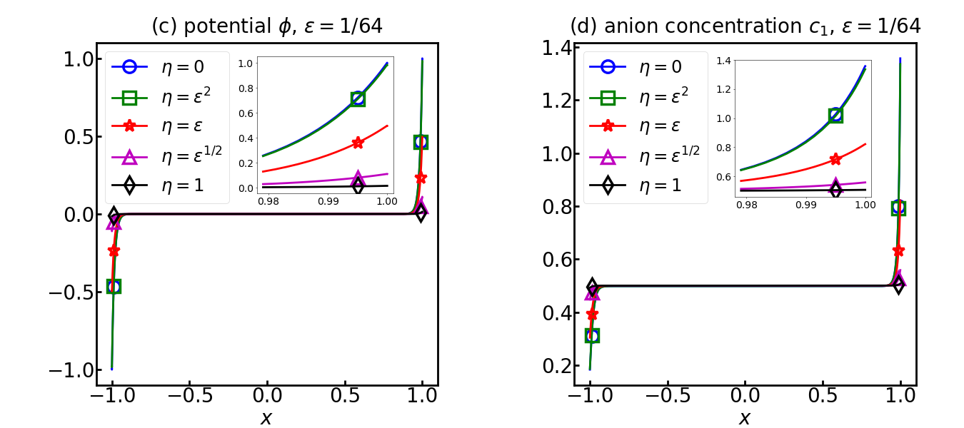
Figure 2: Electroneutral systems, case 2.1, 2.2 in Table 1, potential $\phi$, anion concentration $c_{1}$, large permittivity $\epsilon=1/4$ (a,b), small permitivity $\epsilon=1/64$ (c,d), integral method with Chebyshev points, $N=100$ subintervals.

5.1.3 Electroneutral case 3

This case uses the more realistic values of $\chi_{1},\chi_{2},\eta$ in Table 1 flavell2014conservative . Figure 3 shows the potential $\phi$ and anion concentration $c_{1}$. In this case with small capacitance parameter $\eta$ = 4.63e-5, the Robin boundary conditions are almost Dirichlet boundary conditions, so $\phi(\pm 1)\approx-\phi_{\pm}$ as seen in Fig. 3a. The anions are attracted to the potential maximum at $x=-1$, leading to a boundary layer in the concentration. Note that the concentration boundary value $c_{1}(-1)\approx 21.6$ is higher than in case 1 and case 2; this is attributed to the higher total concentration $a_{1}=2$ in this case. These results agree well with the late time results for the time-dependent PNP equations in Fig. 2 of flavell2014conservative .

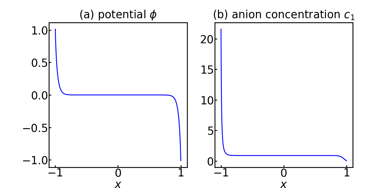
Figure 3: Electroneutral system, case 3 in Table 1, (a) potential $\phi$, (b) anion concentration $c_{1}$, integral method with Chebyshev points, $N=100$ subintervals.

5.2 Non-electroneutral systems

This is case 4 in Table 1. In contrast to previous cases, here the total cation concentration $a_{2}=2$ is greater than the total anion concentration $a_{1}=1$, and the formal potential boundary values are equal, $\phi_{\pm}=1$ lee2010new .

Figure 4 shows the results, where the top frames use large permittivity $\epsilon=1/4$ (case 4.1) and the bottom frames use small permittivity $\epsilon=1/16$ (case 4.2). Five values of the capacitance parameter are considered, $\eta=0,\epsilon^{2},\epsilon,\epsilon^{1/2},1$. Results are shown for the potential $\phi$, potential gradient $\phi^{\prime}$, and ion concentrations $c_{1},c_{2}$ (in this case the concentrations have different profiles). The potential is maximum at $x=0$ and the potential boundary values $\phi(1)$ are printed on the right side of the plots; these results are in good agreement with lee2010new . The high potential at $x=0$ attracts anions and repels cations, leading to boundary layers in the ion concentrations.

As the capacitance parameter $\eta$ increases, the potential also increases, but the profiles have almost the same shape and the potential gradient is almost independent of $\eta$ (the curves overlap); the ion concentrations are also almost independent of $\eta$ because the Nernst-Planck equation (3b) depends on $\phi^{\prime}$, but not $\phi$. As the permittivity $\epsilon$ decreases, the potential gradient and ion concentrations develop sharp boundary layers. In lee2010new it was proven that as $\epsilon\to 0$, the potential $\phi(x)\to\infty$ for all $x\in[-1,1]$ and Fig. 4 is consistent with this. Figure 4 also suggests that the ion concentration boundary values converge like $c_{1}(\pm 1)\to 0,c_{2}(\pm 1)\to\infty$ as $\epsilon\to 0$.

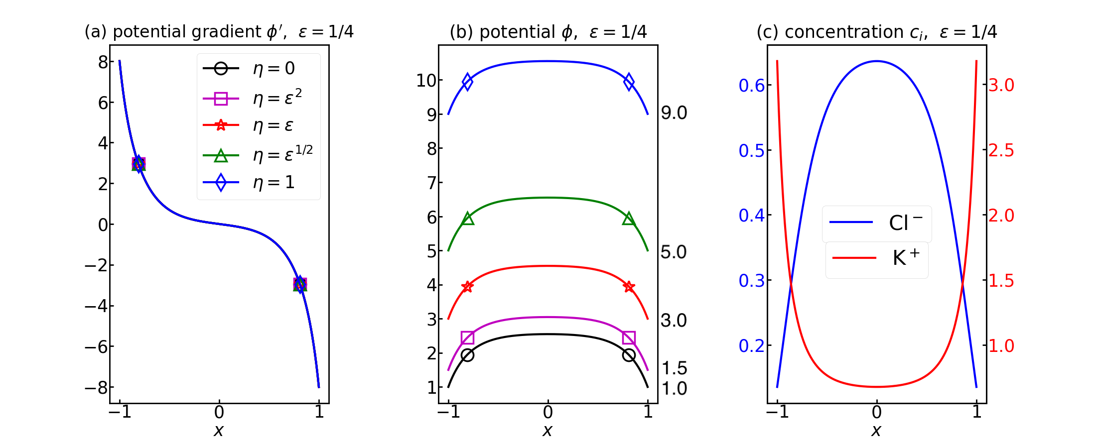
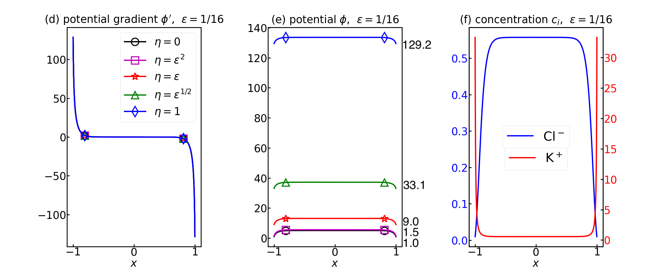
Figure 4: Non-electroneutral systems, case 4.1, 4.2 in Table 1, total concentration $a_{1}=1$ (anion), $a_{2}=2$ (cation), large permittivity $\epsilon=1/4$ (top), small permittivity $\epsilon=1/16$ (bottom), equal formal potential boundary values $\phi_{\pm}=1$, capacitance parameter $\eta=0,\epsilon^{2},\epsilon,\epsilon^{1/2},1$, (a,d) potential $\phi$, (b,e) potential gradient $\phi^{\prime}$, (c,f) ion concentration ($c_{1}$ anion, $c_{2}$ cation), integral method with Chebyshev points, $N=100$ subintervals.

Table 3 shows the potential error and convergence rate confirming 2nd order accuracy $p\approx 2$ for this non-electroneutral system. As before, for large permittivity $\epsilon=1/4$ the uniform and Chebyshev points yield similar results. For small permittivity $\epsilon=1/16$ the number of iterations is higher for both points sets, but Chebyshev points require fewer iterations and yield smaller error.

case 4.1, $\epsilon=1/4$
$N$	uniform			Chebyshev
	iter	error	$p$	iter	error	$p$
50	20	7.4e-2		20	7.2e-3
100	20	1.8e-2	2.039	21	1.8e-3	2.010
200	20	4.5e-3	2.010	21	4.5e-3	2.005
400	21	1.1e-3	2.002	21	1.1e-3	2.001
case 4.2, $\epsilon=1/16$
$N$	uniform			Chebyshev
	iter	error	$p$	iter	error	$p$
50	nc			66	1.5e+0
100	nc			64	3.9e-1	1.940
200	89	4.5e-0		65	9.9e-2	1.978
400	86	8.7e-1	2.359	68	2.3e-2	2.088

Table 3: Non-electroneutral system (case 4.1, 4.2) lee2010new , parameters in Table 1, large permittivity $\epsilon=1/4$, small permittivity $\epsilon=1/16$, $N$ subintervals, uniform and Chebyshev points, number of iterations iter, potential error $\|{\bf\Phi}_{2N}-{\bf\Phi}_{N}\|_{2}$, convergence rate $p$, nc = did not converge.

6 K⁺ ion channel

Finally we consider a potassium (K⁺) ion channel model following gardner2004electrodiffusion . Figure 5 shows a cross-section of the model comprising two conical baths with KCl solvent and a cylindrical channel with four subregions (buffer, nonpolar, central cavity, selectivity filter). In this example the PNP equations are solved in dimensional form with the 1D approximation from gardner2004electrodiffusion ,

$$- A^{-1}\left(\epsilon A\phi^{\prime}\right)^{\prime}=e(z_{1}c_{1}+z_{2}c_{2}-\rho_{n}),$$ (43a)

$$A^{-1}\left(A\left(D_{i}c_{i}^{\prime}+z_{i}\mu_{i}c_{i}\phi^{\prime}\right)\right)^{\prime}=0,$$ (43b)

where $A(x)=\pi r(x)^{2}$ is the cross-sectional area in terms of the radius $r(x)$. Note that the Poisson equation (43a) now includes a density of fixed negative charge $\rho_{n}(x)$. Table 4 gives the parameter values. The model extends over the interval $[-5,8.5]$ (the spatial unit is nm). The four channel subregions have constant radius $r(x)=0.5$, and while gardner2004electrodiffusion took $r(x)$ to be linear in the baths with $r(-5)=r(8.5)=5.5$, here we consider a piecewise constant approximation as suggested by the red dotted lines in Fig. 5; in practice we used 20 steps in each bath. The other parameters are constant in each subregion, where the ion mobility is $\mu_{i}=eD_{i}/k_{B}T$ in terms of the diffusion coefficient $D_{i}$.

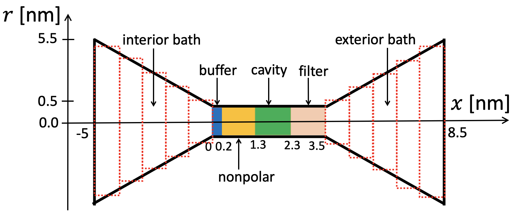
Figure 5: Schematic diagram of K⁺ ion channel model gardner2004electrodiffusion comprising interior/exterior conical baths with KCl solvent and a cylindrical channel with four subregions (buffer, nonpolar, central cavity, selectivity filter), channel subregions have constant radius $r=0.5$ [nm], bath radius is linear (black, solid line) in gardner2004electrodiffusion and piecewise constant (red, dotted line) in present work.

	interval	$\ell$	$r(x)$	$A(x)$	$Q$	$\rho_{n}$	$\epsilon$	$\mu_{i}$	$D_{i}$
interior bath	[-5.0, 0.0]	5	see text	$\pi r(x)^{2}$	0	0	80	60	1.5
buffer	[0.0, 0.2]	0.2	0.5	$\pi$/4	-4	$80/\pi$	80	16	0.4
nonpolar	[0.2, 1.3]	1.1	0.5	$\pi$/4	0	0	4	16	0.4
central cavity	[1.3, 2.3]	1	0.5	$\pi$/4	-1/2	$2/\pi$	30	16	0.4
selectivity filter	[2.3, 3.5]	1.2	0.5	$\pi$/4	-3/2	$5/\pi$	30	16	0.4
exterior bath	[3.5, 8.5]	5	see text	$\pi r(x)^{2}$	0	0	80	60	1.5

Table 4: K⁺ channel parameters gardner2004electrodiffusion , interval [nm], length $\ell$ [nm], radius $r(x)$ [nm], cross-sectional area $A(x)$ [nm]², total fixed charge $Q~{}[e]$, fixed charge density $\rho_{n}$ [molar], permittivity $\epsilon$, mobility $\mu_{i}=eD_{i}/k_{B}T$ [1e-5 cm²/(V $\cdot$ s)], diffusion coefficient $D_{i}$ [1e-5 cm²/s].

The potential and ion concentrations satisfy Dirichlet boundary conditions,

$$\phi(-5) =0,\quad\phi(8.5)=-100\;{\text{mV}},$$ (44a)

$$c_{i}(-5) =c_{i}(8.5)=0.15\;{\text{molar}},\quad i=1,2.$$ (44b)

There are five interfaces, $x=0,0.2,1.3,2.3,3.5$, at which the potential and ion concentrations satisfy continuity conditions,

$$[\phi]=0,\quad\left[\epsilon A\phi^{\prime}\right]=0,$$ (45a)

$$[c_{i}]=0,\quad\left[A\left(D_{i}c_{i}^{\prime}+z_{i}\mu_{i}c_{i}\phi^{\prime}\right)\right]=0,$$ (45b)

where the bracket indicates the jump across the interface.

The integral method previously described for systems with one domain was extended to this example with six domains (two baths, four channel subregions) and the scheme has the same Gummel iteration form as (39). In this case the computations used uniform grid spacing $h=0.01$ and the same stopping criterion as before (41). Note that the mobility to diffusion coefficient ratio is $\mu_{i}/D_{i}=40$, which implies that the K⁺ ion channel problem is drift-dominated (43b), so in this case we used a continuation scheme; the problem was solved for an increasing sequence of ratios, $\mu_{i}/D_{i}=1,10,20,40$, with relaxation parameters $\omega=0.9,0.4,0.26,0.18$, and requiring 12, 69, 148, 218 iterations, respectively, where the converged solution for one ratio $\mu_{i}/D_{i}$ is the initial guess for the next ratio; the total run time for all four ratios was 44 seconds. The continuation scheme was not needed for the electroneutral and non-electroneutral systems considered earlier since the ratio $\mu_{i}/D_{i}$ was much smaller in those examples.

Figure 6 shows the computed potential and ion concentration profiles which agree well with the previous results gardner2004electrodiffusion . The negative fixed charge density $\rho_{n}$, indicated by green dashed lines, has substantial impact on the potential and ion concentrations. In particular, the polar subregions with negative fixed charge have local potential minima below the boundary potential (-133.7 mV in the buffer, -155.8 mV in the filter), while the potential rises to a local maximum in the nonpolar subregion (-34.3 mV). As a result, the K⁺ cations are attracted to the buffer and filter, and are expelled from the nonpolar region, while the opposite is true for the Cl^- anions; this demonstrates the cation selectivity property of the K⁺ channel.

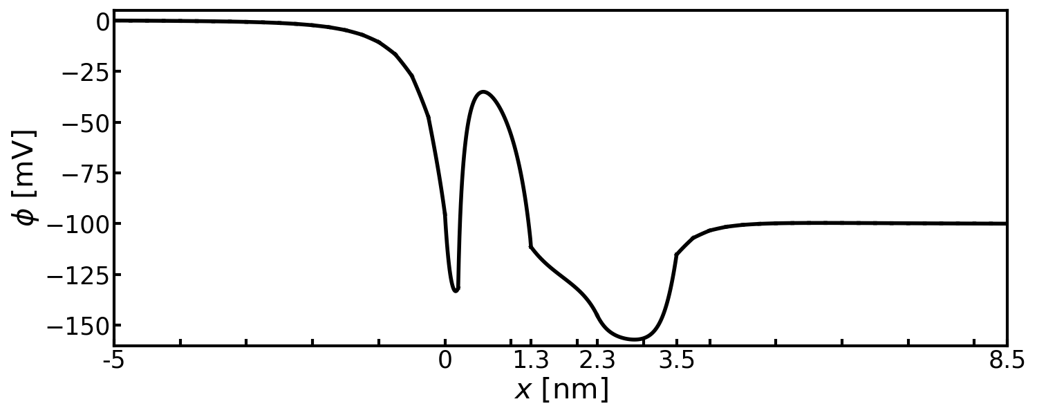
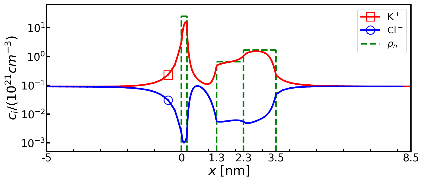
Figure 6: K⁺ ion channel model depicted in Fig. 5 gardner2004electrodiffusion , parameters in Table 4, Dirichlet boundary conditions (44), fixed negative charge density $\rho_{n}$ (green dashed lines), (a) potential $\phi$ [mV], (b) ion concentration $c_{i}$ [molar], K⁺ (red solid line), Cl^- (blue solid line), integral equation method with uniform points, grid spacing $h=0.01$.

We also computed the current-voltage curve for the K⁺ channel model, where the current is

$$I(V_{\rm app}) =-\sum_{i=1}^{2}z_{i}eA(D_{i}c_{i}^{\prime}+z_{i}\mu_{i}c_{i}\phi^{\prime}),$$ (46a)

$$V_{\rm app} =\phi(-5)-\phi(8.5),$$ (46b)

in terms of the applied voltage $V_{\rm app}$ across the channel. All other parameters are the same as in Table 4. It follows from the NP equation (43b) that the current (46a) is constant throughout the domain and in the present calculations this was satisfied to machine precision.

Figure 7 shows the computed I-V curve which closely matches the expected linear relation. For $V_{\rm app}$ = 100 mV the current is $I$ = 19.4 pA, which comprises 19.1 pA for K⁺ cations and 0.3 pA for Cl^- anions, which again shows the cation selectivity of the K⁺ channel. For comparison, gardner2004electrodiffusion obtained 22.2 pA for cations and 0.3 pA for anions. In the present case, we checked that the computed current is not sensitive to the number of steps in the bath region, while Table 5 shows that the value approaches the result in gardner2004electrodiffusion as the grid spacing $h$ is reduced.

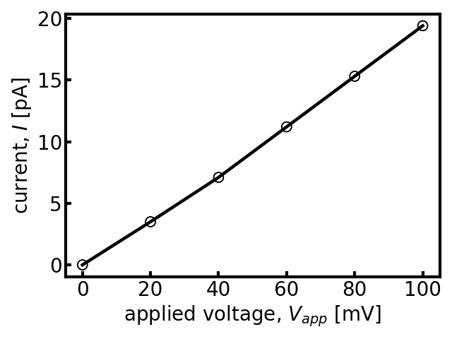
Figure 7: K⁺ ion channel, parameters in Table 4 gardner2004electrodiffusion , current $I$ [pA] versus applied voltage $V_{\rm app}$ [mV], grid spacing $h=0.01$ nm.

$h$ nm	0.02	0.01	0.005	0.0025	0.00125
$I$ pA	14.68	19.39	20.50	20.78	20.86

Table 5: K⁺ ion channel model gardner2004electrodiffusion , applied voltage $V_{\rm app}$ = 100 mV, computed current $I$ [pA] versus grid spacing $h$ [nm].

7 Summary

An integral equation method was presented for the 1D steady-state PNP equations modeling ion transport through membrane channels. Green’s 3rd identity was applied to recast the PNP differential equations as a fixed-point problem involving integral operators for the potential gradient and ion concentrations. The integrals were computed by midpoint and trapezoid rules at either uniform or Chebyshev grid points, and the resulting nonlinear equations were solved by Gummel iteration with relaxation. Each iteration requires solving a small linear system for the boundary and interface variables.

The integral equation method was applied to electroneutral and non-electroneutral systems with Robin boundary conditions on the potential and no-flux boundary conditions on the ion concentrations. The method is 2nd order accurate even in cases with sharp boundary layers. The method was also applied to a drift-dominated K⁺ ion channel model following gardner2004electrodiffusion . In this case the fixed charge density in the channel ensures the selectivity of K⁺ ions and exclusion of Cl^- ions. In these tests the integral method results agree well with published finite-difference and finite-element results lee2010new ; flavell2014conservative ; gardner2004electrodiffusion .

Various techniques are have been used in numerical PNP solvers to improve stability such as positivity-preserving schemes, Slotboom variables, and streamwise upstream differencing. The integral method calculations presented here did not employ these techniques, although it did use relaxation to accelerate the iteration and continuation to compute a good initial guess for drift-dominated systems. It is noteworthy that in these calculations, the integral method preserved the positivity of the ion concentrations.

In future work we aim to extend the integral equation PNP solver to time-dependent problems as well as 2D and 3D ion channel models, where the volume integral can be efficiently computed using adaptive quadrature and a fast summation method wang2020kernel ; wilson2022tabi ; xu2023dynamics .

Acknowledgments This work was supported by NSF grants DMS-1819094/1819193 and DMS-2110767/2110869.

Declarations

Conflict of interest The authors declare that they have no conflict of interest.

Data availability The datasets generated during the current study can be replicated by running the Python scripts in the BIE_PNP_1D repository, https://github.com/zhen-wwu.

References

- \bibcommenthead
- (1) Hille, B.: Ionic channels in excitable membranes. Current problems and biophysical approaches. Biophys. J. 22, 283–294 (1978)
- (2) Hille, B.: Ion Channels of Excitable Membranes. Sinauer, 3rd edition (2001)
- (3) Liu, X., Lu, B.: Incorporating Born solvation energy into the three-dimensional Poisson–Nernst–Planck model to study ion selectivity in KcsA K+ channels. Phys. Rev. E 96, 062416 (2017)
- (4) Eisenberg, B., Liu, W.: Poisson–Nernst–Planck systems for ion channels with permanent charges. SIAM J. Math. Anal. 38, 1932–1966 (2007)
- (5) Horng, T.-L., Lin, T.-C., Liu, C., Eisenberg, B.: PNP equations with steric effects: a model of ion flow through channels. J. Phys. Chem. B 116, 11422–11441 (2012)
- (6) Xie, D., Chao, Z.: A finite element iterative solver for a PNP ion channel model with Neumann boundary condition and membrane surface charge. J. Comput. Phys. 423, 109915 (2020)
- (7) Wang, Q., Li, H., Zhang, L., Lu, B.: A stabilized finite element method for the Poisson-Nernst-Planck equations in three-dimensional ion channel simulations. Appl. Math. Lett. 111, 106652 (2021)
- (8) Zheng, Q., Chen, D., Wei, G.-W.: Second-order Poisson-Nernst-Planck solver for ion transport. J. Comput. Phys. 230, 5239–5262 (2011)
- (9) Flavell, A., Machen, M., Eisenberg, B., Kabre, J., Liu, C., Li, X.: A conservative finite difference scheme for Poisson-Nernst-Planck equations. J. Comput. Electron. 13, 235–249 (2014)
- (10) Lu, B., Zhou, Y., Huber, G.A., Bond, S.D., Holst, M.J., McCammon, J.A.: Electrodiffusion: a continuum modeling framework for biomolecular systems with realistic spatiotemporal resolution. J. Chem. Phys. 127(13), 10–604 (2007)
- (11) Lu, B., Holst, M.J., Andrew McCammon, J., Zhou, Y.C.: Poisson-Nernst-Planck equations for simulating biomolecular diffusion–reaction processes I: Finite element solutions. J. Comput. Phys. 229, 6979–6994 (2010)
- (12) Xie, D., Lu, B.: An effective finite element iterative solver for a Poisson-Nernst-Planck ion channel model with periodic boundary conditions. SIAM J Sci Comput. 42(6), 1490–1516 (2020)
- (13) Chainais-Hillairet, C., Peng, Y.-J.: Convergence of a finite–volume scheme for the drift–diffusion equations in 1D. IMA J. Numer. Anal. 23, 81–108 (2003)
- (14) Song, Z., Cao, X., Huang, H.: Electroneutral models for dynamic Poisson-Nernst-Planck systems. Phys. Rev. E 97, 012411 (2018)
- (15) Song, Z., Cao, X., Horng, T.-L., Huang, H.: Selectivity of the KcsA potassium channel: Analysis and computation. Phys. Rev. E 100, 022406 (2019)
- (16) Hu, J., Huang, X.: A fully discrete positivity–preserving and energy-dissipative finite difference scheme for Poisson-Nernst-Planck equations. Numer. Math. 145, 77–115 (2020)
- (17) Steinbach, O.: Numerical Approximation Methods for Elliptic Boundary Value Problems: Finite and Boundary Elements. Springer Science+Business Media, LLC (2008)
- (18) Juffer, A., Botta, E.F., van Keulen, B.A., van der Ploeg, A., Berendsen, H.J.: The electric potential of a macromolecule in a solvent: A fundamental approach. J. Comput. Phys. 97, 144–171 (1991)
- (19) Geng, W., Krasny, R.: A treecode-accelerated boundary integral Poisson-Boltzmann solver for electrostatics of solvated biomolecules. J. Comput. Phys. 247, 62–78 (2013)
- (20) Barcilon, V., Chen, D.-P., Eisenberg, R.: Ion flow through narrow membrane channels: Part II. SIAM J. Appl. Math. 52, 1405–1425 (1992)
- (21) Gardner, C.L., Nonner, W., Eisenberg, R.S.: Electrodiffusion model simulation of ionic channels: 1D simulations. J. Comput. Electron. 3, 25–31 (2004)
- (22) Gummel, H.K.: A self–consistent iterative scheme for one–dimensional steady state transistor calculations. IEEE Trans. Electron. Devices 11, 455–465 (1964)
- (23) Jerome, J.W.: Consistency of semiconductor modeling: an existence/stability analysis for the stationary van Roosbroeck system. SIAM J. Appl. Math. 45, 565–590 (1985)
- (24) Greengard, L., Rokhlin, V.: On the numerical solution of two-point boundary value problems. Commun. Pure Appl. Math. 44, 419–452 (1991)
- (25) Viswanath, D., Tobasco, I.: Navier-Stokes solver using Green’s functions I: Channel flow and plane Couette flow. J. Comput. Phys. 251, 414–431 (2013)
- (26) Lee, C.-C., Lee, H., Hyon, Y., Lin, T.-C., Liu, C.: New Poisson-Boltzmann type equations: one-dimensional solutions. Nonlinearity 24, 431 (2010)
- (27) Wang, L., Krasny, R., Tlupova, S.: A kernel-independent treecode based on barycentric Lagrange interpolation. Commun. Comput. Phys. 28, 1415–1436 (2020)
- (28) Wilson, L., Geng, W., Krasny, R.: TABI-PB 2.0: An improved version of the treecode-accelerated boundary integral Poisson-Boltzmann solver. J. Phys. Chem. B 126, 7104–7113 (2022)
- (29) Xu, L., Krasny, R.: Dynamics of elliptical vortices with continuous profiles. Phys. Rev. Fluids 8, 024702 (2023)