Local diabatic representation of conical intersection quantum dynamics

Abstract

Conical intersections are ubiquitous in polyatomic molecules and responsible for a wide range of phenomena in chemistry and physics. We introduce and implement a local diabatic representation for the correlated electron-nuclear dynamics around conical intersections. It employs the adiabatic electronic states but avoids the singularity of nonadiabatic couplings, and is robust to different gauge choices of the electronic wavefunction phases. Illustrated by a two-dimensional conical intersection model, this representation captures nonadiabatic transitions, electronic coherence, and geometric phase.

I Introduction

Conical intersection (CI), degeneracy points in the adiabatic potential energy surfaces, is ubiquitous in polyatomic molecules. It is responsible for virtually all photochemical and photophysical processes including nonradiative relaxation, Jahn-Teller effect, vision, photo-stability of DNA molecules [1, 2, 3, 4, 5]. In the vicinity of CIs, the electronic and nuclear motion becomes strong coupled, thus the adiabatic Born-Oppenheimer approximation breaks down. An immediate consequence of the strong electron-nuclear (vibronic) coupling is the nonradiative electronic relaxation. Furthermore, transient electronic coherences may emerge during the passage through a CI. It has been suggested that such transient coherence can be probed by stimulated x-ray Raman scattering [6, 7] and twisted x-ray diffraction [8], which can provide a direct spectroscopic signature of CIs.

Another effect due to CI is geometric phase [9, 10, 1]. A nuclear trajectory encircling a CI in the configuration space will pick up a geometric phase [11]. The geometric phase arises not only in the nonadiabatic dynamics, but also in the adiabatic dynamics even when the CI is energetically inaccessible. This has been observed experimentally in the H + HD $\rightarrow$ H2 + D reaction [12]. Incorporating the geometric phase into the molecular dynamics is essential to understand the adiabatic and nonadiabatic molecular dynamics [13].

Understanding the CI dynamics requires solving the nuclear wave packet dynamics in multiple electronic potential energy surfaces [14]. This is usually done with exact quantum dynamics approaches in ab initio computed potential energy surfaces [15]. Approximate methods with a classical treatment of nuclei including the widely used trajectory surface-hopping [16] and Ehrenfest dynamics [17], being useful to describe electronic relaxation dynamics in large-scale molecular systems, cannot describe properly the transient electronic coherence and geometric phase [15, 18]. The nonadiabatic conical intersection dynamics is either performed in the adiabatic or the diabatic representation. In the adiabatic representation, the Born-Huang ansatz is used for the molecular wavefunction, $\Psi(\mathbf{r},\mathbf{R},t)=\sum_{\alpha}{\phi_{\alpha}(\mathbf{r};\mathbf{R})}\chi_{\alpha}(\mathbf{R},t)$ where $\phi_{\alpha}(\mathbf{r};\mathbf{R})$ is the $\alpha$th adiabatic electronic state depending parametrically on the nuclear configuration $\mathbf{R}$ and $\chi_{\alpha}(\mathbf{R},t)$ is the associated nuclear wave packet. This leads to the intuitive picture of each nuclear wave packet propagating in its own adiabatic potential energy surfaces (APES) and makes electronic transitions when it encounters a region in the configuration space where the nonadiabatic couplings becomes significant, e.g. close to a CI. The gauge freedom in the Born-Huang approach is a local U(1) phase transformation ${\chi_{\alpha}^{\prime}}(\mathbf{R})=e^{i\theta_{\alpha}(\mathbf{R})}{\chi_{\alpha}(\mathbf{R})},{\phi_{\alpha}^{\prime}}(\mathbf{r};\mathbf{R})=e^{-i\theta_{\alpha}(\mathbf{R})}{\phi_{\alpha}}(\mathbf{r};\mathbf{R})$. In this representation, the nonadiabatic coupling accounts for all nonadiabatic effects. Note that the nuclear wave packets are gauge-dependent and thus cannot be experimentally observed. A major problem running quantum dynamics on the adiabatic potential energy surfaces is that in the presence of CI, the nonadiabatic coupling becomes singular. This is because the nonadiabatic coupling depends inversely on the energy gap and the gap vanishes at the CI point where two APESs intersect.

Transforming to the diabatic representation can avoid such singularities, whereby the couplings between diabatic states are well-behaved functions of nuclear coordinates. In fact, there are quantum dynamics methods that can only be used under the diabatic representation [19]. However, exact diabatization in general does not exist within a finite number of electronic states due to topological obstruction [20]. Various approximate quasi-diabatization methods have been proposed [21, 22] based on different criteria. This may introduce spurious singularities or require further approximations [21]. For example, in the adiabatic-to-diabatic transformation approach, the residual couplings, the part of nonadiabatic couplings that cannot be transformed into diabatic couplings, are usually neglected [23].

Here we propose a locally diabatic representation (LDR) for the coupled electron-nuclear quantum dynamics at a CI. This representation avoids the singularity of nonadiabatic couplings because the nuclear kinetic energy operator does not operate on the electronic states. Moreover, while being a diabatic representation, it employs the adiabatic electronic eigenstates. Thus, it is straightforward to combine it with the well-established quantum chemistry methods, that usually computes the adiabatic electronic states at a fixed nuclear geometry. The LDR can be taken as a generalization of the crude adiabatic representation, wherein electronic states at a single reference nuclear configuration are chosen as the basis set[24]. This representation is crude in the sense that the chosen electronic basis will not be appropriate when the nuclear configuration deviates far from the reference geometry. In the LDR, many reference nuclear configurations, determined by a discrete variable representation of the nuclear coordinates, are chosen. The nonadiabatic transitions and geometric phase effects are all included in an electronic overlap matrix, the overlap between electronic states at different nuclear geometries. This overlap matrix is always well-behaved, even when the adiabatic electronic states are not smooth with respect to the nuclear coordinates. Therefore, the adiabatic states obtained from electronic structure computations can be directly used without further smoothing procedure. An illustration of the utility of LDR is made for modeling the nonadiabatic wave packet dynamics of a two-dimensional CI model.

II Local Diabatic Representation

The LDR is constructed as follows. In contrast to the adiabatic representation, we consider the nuclear motion first and then electronic. We choose a primitive basis set $\set{\chi_{\mu}(\mathbf{R})}$ of size $N$, not necessarily orthogonal, to describe the nuclear motion. This basis set should cover the relevant nuclear configuration space of the target process. We then construct the localized orthogonal basis functions by solving a generalized eigenvalue problem of the position operators. Since all position operators commute, they share common eigenstates labeled by their eigenvalues $\ket{\mathbf{R}_{n}}$ with $n$ running over the eigenstates . Expand $\ket{\mathbf{R}_{n}}=\sum_{\mu}U_{\mu n}\ket{\chi_{\mu}}$, the transformation matrix can be obtained by solving the eigenvalue problem for each position operator $x$

$$XU=SU\Lambda,$$ (1)

$X_{\mu\nu}=\braket{\chi_{\mu}}{x}{\chi_{\nu}}$, $S_{\mu\nu}=\braket{\chi_{\mu}}{\chi_{\nu}}$ is the nuclear overlap matrix, and the diagonal matrix $\Lambda$ contains the position eigenvalues. This basis set defines a resolution of identity of the nuclear space $I=\sum_{\mu,\nu}\ket{\chi_{\mu}}\mathinner{\left(S^{-1}\right)}_{\mu\nu}\bra{\chi_{\nu}}=\sum_{n}\ket{\mathbf{R}_{n}}\bra{\mathbf{R}_{n}}$.

Our ansatz for the full molecular wavefunction is now given by

$$\begin{split}\Psi(\mathbf{r},\mathbf{R},t)&=\sum_{n}\Phi_{n}(\mathbf{r},t;\mathbf{R}_{n})\chi_{n}(\mathbf{R})\\ &=\sum_{n}{\sum_{\alpha}C_{n\alpha}(t)\phi_{\alpha}(\mathbf{r};\mathbf{R}_{n})}\chi_{n}(\mathbf{R};\mathbf{R}_{n})\end{split}$$ (2)

where $\chi_{n}(\mathbf{R})=\braket{\mathbf{R}}{\mathbf{R}_{n}}$ is a nuclear wave function centered at $\mathbf{R}_{n}$, $\phi_{\alpha}(\mathbf{r},\mathbf{R}_{n})$ is the $\alpha$th adiabatic electronic state $H_{\text{BO}}(\mathbf{R}_{n})\phi_{\alpha}(\mathbf{r};\mathbf{R}_{n})=E_{\alpha}(\mathbf{R}_{n})\phi(\mathbf{r};\mathbf{R}_{n})$ with $H_{\text{BO}}(\mathbf{R})=H-\hat{T}_{\text{n}}$ the electronic Hamiltonian, the full molecular Hamiltonian subtracting the nuclear kinetic energy operator. Here $E_{\alpha}(\mathbf{R})$ are the adiabatic potential energy surfaces.

In comparison to the adiabatic representation, the ansatz reverses the role of electrons and nuclei: instead of thinking about a time-dependent nuclear wave packet associated with a fixed APES, we consider a time-dependent electronic state $\Phi_{n}(\mathbf{r},t;\mathbf{R}_{n})$ associated with a fixed nuclear basis. In the second step of Eq. (2), we have expanded the electronic state in terms of the adiabatic electronic basis at a reference geometry defined by the associated nuclear basis. This ansatz can then be understood as an expansion of the full molecular wavefunction in terms of the electron-vibrational (vibronic) basis set $\set{\phi_{\alpha}(\mathbf{r};\mathbf{R}_{n})\chi_{n}(\mathbf{R})}$ with expansion coefficients $C_{n\alpha}(t)$. Following the orthonormality of the nuclear basis set, the vibronic basis set is also orthonormal in the joint electron-nuclear space, i.e., $\braket{\phi_{\beta}(\mathbf{R}_{m}),\mathbf{R}_{m}}{\phi_{\alpha}(\mathbf{R}_{n}),\mathbf{R}_{n}}=\delta_{\beta\alpha}\delta_{nm}$.

There is a gauge structure in Eq. (2),

$$\ket{\mathbf{R}_{n}^{\prime}}=e^{i\theta_{n}}\ket{\mathbf{R}_{n}},~{}~{}~{}\ket{\phi_{\alpha}^{\prime}(\mathbf{R}_{n})}=e^{-i\theta_{n}}\ket{\phi_{\alpha}(\mathbf{R}_{n})}.$$ (3)

This is a discretized form of the gauge transformation in the Born-Huang expansion, $U=e^{i\theta(\mathbf{R})}$. However, while $\theta(\mathbf{R})$ is required to be continuous function of $\mathbf{R}$ in the Born-Huang approach, the $\theta_{n}$ can be independently and arbitrarily chosen. This is because, as will be shown below, our dynamical equation does not involve nuclear derivative of the electronic wavefunctions.

Inserting Eq. (2) into the time dependent Schrödinger equation for the molecule $i\dfrac{\partial{}\Psi}{\partial{t}}=\mathinner{\left(H_{\text{BO}}+\hat{T}_{\text{n}}\right)}\Psi$ and left multiply $\bra{\psi_{\beta}(\mathbf{R}_{m})}\bra{\mathbf{R}_{m}}$ yields

$$i\dot{C}_{m\beta}(t)=E_{\beta}(\mathbf{R}_{m})C_{m\beta}(t)+T_{mn}A_{m\beta,n\alpha}C_{n\alpha}$$ (4)

where we have made use of

$$H_{\text{BO}}(\mathbf{R})\ket{\psi_{n}(\mathbf{R}_{\alpha})}\ket{\mathbf{R}_{\alpha}}=E_{n}(\mathbf{R}_{\alpha})\ket{\psi_{n}(\mathbf{R}_{\alpha})}\ket{\mathbf{R}_{\alpha}}.$$ (5)

Here $T_{\beta\alpha}=\braket{\mathbf{R}_{\beta}}{\hat{T}_{\text{n}}}{\mathbf{R}_{\alpha}}_{\mathbf{R}}$ is the kinetic energy operator matrix elements and the electronic overlap matrix

$$A_{m\beta,n\alpha}=\braket{\psi_{m}(\mathbf{R}_{\beta})}{\psi_{n}(\mathbf{R}_{\alpha})}_{\mathbf{r}},$$ (6)

where $\braket{\cdots}_{\mathbf{r}}$ ($\braket{\cdots}_{\mathbf{R}}$) denotes the integration over electronic (nuclear) degrees of freedom. In Eq. (5), we have employed an approximation used in the discrete variable representation [25] $\braket{\mathbf{R}_{n}}{V(\mathbf{R})}{\mathbf{R}_{n}}\approx V(\mathbf{R}_{n})$.

Eq. (4) can also be derived by Dirac-Frenkel variational principle $\delta\int_{t_{i}}^{t_{f}}\operatorname{d\!}t\braket{\Psi}{i\partial_{t}-H}{\Psi}=0$. The first term in the right-hand side of Eq. (4) gives a dynamical phase depending on the APESs. The electronic overlap matrix $A$ appearing in the second term encodes all nonadiabatic effects and geometric phase. It plays a similar role to nonadiabatic coupling in the adiabatic representation. For any $n$, $A_{n\beta,n\alpha}=\delta_{\beta\alpha}$ due to orthonormality of the adiabatic electronic states. Also, it is Hermitian

$$A_{m\beta,n\alpha}=A_{n\alpha,m\beta}^{*}$$ (7)

The overlap matrix is gauge-dependent, and transform as $A^{\prime}_{m\beta,n\alpha}=A_{m\beta,n\alpha}e^{-i\mathinner{\left(\theta_{n}-\theta_{m}\right)}}$ under the gauge transformation in Eq. (3). But consider a loop encircling a CI with geometries labeled by $1,2,\cdots,N$, the Wilson loop $W_{\alpha}=A_{1\alpha,2\alpha}A_{2\alpha,3\alpha}\cdots A_{N\alpha,1\alpha}$ reflects the geometric phase and is gauge invariant [26].

The expansion coefficients for different electronic states becomes decoupled in the limit where $A_{m\beta,n\alpha}\approx A_{mn}^{\alpha}\delta_{\beta\alpha}$. This implies that the ground electronic state at $\mathbf{R}$ and excited electronic state at $\mathbf{R}^{\prime}\neq\mathbf{R}$ are orthogonal. In other words, let $\mathbf{R}^{\prime}=\mathbf{R}+\Delta\mathbf{R}$, $\braket{\phi_{g}(\mathbf{R})}{\phi_{e}(\mathbf{R}+\Delta\mathbf{R})}=\Delta\mathbf{R}\cdot\braket{\phi_{g}(\mathbf{R})}{\nabla_{\mathbf{R}}}{\phi_{e}(\mathbf{R})}=0$. Thus, this approximation is equivalent to neglecting the nonadiabatic couplings, the LDR is consistent with the adiabatic representation in this limit. However, the geometric phase effects in the adiabatic dynamics is still captured by $A_{mn}^{\alpha}$.

Eq. (4) offers several advantages for nonadiabatic quantum dynamics simulations. First, although we have employed the adiabatic electronic states, it does not contain any singularities because the nuclear kinetic energy operator does not operate on the electronic states. Therefore, in contrast to wave packet dynamics in the adiabatic representation, the singularity of the nonadiabatic coupling at the CI point will not affect the simulations. In fact, the CI configuration can be safely included in our basis set. Moreover, Eq. (4) can be used for an arbitrary gauge. It does not require the electronic wavefunction to be continuous with respect to the nuclear geometry because there is no term involving the nuclear derivative of the electronic wavefunction. This is advantages for quantum dynamics simulations as electronic structure calculations at different geometries can be directly used without further smoothing procedure.

In practice, the nuclear kinetic energy matrix elements can be analytically calculated within the primitive basis and then transformed into the position eigenstates. The adiabatic electronic states can be computed with well-established electronic structure methods. Any nuclear basis set can be used. Depending on the nuclear degree of freedom, different basis may be more convenient and require less basis functions to converge than the other. For example, a Fourier basis may be convenient for rotational dynamics (e.g. in isomerization) whereas local Gaussian bases including coherent states may be useful for describing vibrational dynamics. When a localized basis set is parameterized by a configuration (e.g. the Gaussian basis is parameterized by a center), it is possible to directly employ the adiabatic electronic states defined at the corresponding configurations, as in the moving crude adiabatic representation [13]. This can also avoid the singular nonadiabatic couplings, but the vibronic basis set are not orthogonal and may encounter singular overlap matrix.

The electronic and nuclear operators in the LDR can be constructed from the resolution of identity of the joint electron-nuclear space, $\mathcal{I}=\sum_{n,\alpha}\ket{\phi_{\alpha}(\mathbf{R}_{n}),\mathbf{R}_{n}}\bra{\phi_{\alpha}(\mathbf{R}_{n}),\mathbf{R}_{n}}.$ This follows from the orthonormality of the basis set and can be verified by $\mathcal{I}\ket{\Psi}=\ket{\Psi}$ for any vibronic state $\Psi$. For a joint electron-nuclear operator $O(\mathbf{r},\mathbf{R})$,

$$\begin{split}O&=\mathcal{I}O\mathcal{I}\\ &=\sum_{m,n}\sum_{\beta,\alpha}O_{m\beta,n\alpha}\ket{\phi_{\beta}(\mathbf{R}_{m}),\mathbf{R}_{m}}\bra{\phi_{\alpha}(\mathbf{R}_{n}),\mathbf{R}_{n}}\\ \end{split}$$ (8)

where $O_{m\beta,n\alpha}=\braket{\phi_{\beta}(\mathbf{R}_{m}),\mathbf{R}_{m}}{O}{\phi_{\alpha}(\mathbf{R}_{n}),\mathbf{R}_{n}}$. The electronic and nuclear reduced density matrices read, respectively, $\rho_{\text{e}}(t)=\sum_{n}C_{n\alpha}(t)C_{n\beta}^{*}(t)\ket{\phi_{\alpha}(\mathbf{R}_{n})}\bra{\phi_{\beta}(\mathbf{R}_{n})}$ and $\rho_{\text{n}}(t)=\sum_{n,m}\sum_{\beta,\alpha}C_{m\beta}^{*}A_{m\beta,n\alpha}C_{n\alpha}\ket{\mathbf{R}_{n}}\bra{\mathbf{R}_{m}}$. For a purely electronic (nuclear) observable $O$, the expectation value can be simplified as $\braket{O(t)}=\sum_{n,\beta\alpha}C_{n\beta}^{*}O^{n}_{\beta\alpha}C_{n\alpha}$ ($\braket{O(t)}=\sum_{m,n}\sum_{\beta,\alpha}C^{*}_{m\beta}O_{mn}A_{m\beta,n\alpha}C_{n\alpha}$).

III Application to conical intersection model

We demonstrate the utility of the LDR for nonadiabatic wavepacket dyn amics by a two-state two-dimensional conical intersection model. The Hamiltonian reads

$$H=\sum_{\sigma=x,y}\mathinner{\left(a_{\sigma}^{\dagger}a_{\sigma}+\frac{1}{2}\right)}-\kappa x\sigma_{z}+\lambda y\sigma_{x}+\Delta\sigma^{+}\sigma^{-}$$ (9)

where $\sigma_{x}=\ket{0}\bra{1}+\ket{1}\bra{0}$ and $\sigma_{z}=\ket{1}\bra{1}-\ket{0}\bra{0}$, $\ket{0},\ket{1}$ are two diabatic states. The adiabatic potential energy surfaces are depicted in fig. 1a, with a CI located at $(x,y)=(0,0)$. The tuning $x$ tunes the energy gap and the coupling $y$ induces electronic transitions. Quantum dynamics of the diabatic vibronic Hamiltonian can be modeled exactly by a split-operator method with the nuclear wave packets associated with each electronic state represented in a numerical grid [27]. Initially, the molecular state is $\Psi_{0}={\pi}^{-1/2}e^{-\frac{1}{2}(x+1)^{2}-\frac{1}{2}y^{2}}\ket{1}\bra{1}$, arising from a vertical excitation from the ground state.

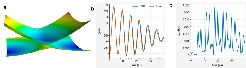
Figure 1: Wave packet dynamics of a two-dimensional conical intersection model. (a) Adiabatic potential energy surfacs. (b) Expectation value of the position operator $x$ reflecting the wavepacket motion. (c) Electronic coherence at a point near conical intersection. The parameters of the model are chosen as (atomic units) $\kappa=1,\lambda=0.2,\Delta=1$.

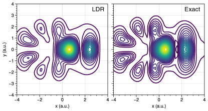
Figure 2: Geometric phase in the total nuclear probability density at $t=40$ a.u.. The geometric phase is reflected in the nodal line along $y=0.$

Here we use coherent states as the primitive nuclear basis set, whereby the matrix elements of position and momentum operators can be analytically calculated. Eq. (4) is solved with the fourth-order Runge-Kutta integrator. fig. 1b shows the expectation value of the tuning mode, which reflects the wave packet motion. The oscillations reflect multiple passages through the CI. The electronic coherence are reflected in the off-diagonal elements of $C(\mathbf{R})=\ket{g(\mathbf{R})}\bra{e(\mathbf{R})}$. fig. 1c shows the electronic coherence at a point close to the CI. The geometric phase effects lead to a nodal line in the nuclear probability density, see Fig. (2). Here the LDR employs adiabatic states, obtained by diaganolizing the electronic Hamiltonian at eigenvalues of the position operators, with an random phase assigned. The CI point is included in our basis set. The results simulated with LDR are in excellent agreement with the exact quantum results.

IV summary

To summarize, we have developed a locally diabatic representation for the correlated electron-nuclear quantum dynamics around conical intersections. It employs the adiabatic electronic states without the diabatization and without introducing the nonadiabatic coupling into the dynamical equations, thus avoiding the singularity associated with conical intersections. By a two-dimensional CI model, we have demonstrated that it can describe accurately the nuclear wave packet passing through a CI, with results in excellent agreement with exact quantum dynamics. The LDR can be useful for problems involving degenerate electronic states. This occurs not only due to conical intersections but also due to spin, for example, in intersystem crossing. This paves the way for ab initio nonadiabatic wave packet dynamics and molecular spectroscopy simulations.

The locally diabatic representation can be generalized to describe any fiber bundle structure [20, 28], which are recognized to be important in many areas of quantum physics, molecular science, and optics. The base space of a bundle will be described within a finite basis representation. After transforming to the localized basis $\set{X_{n}}$, an adiabatic representation ${F\mathinner{\left(X_{n}\right)}}$ is used for the fiber associated with the basis $X_{n}$. That is, the full space is covered with a set of product spaces ${F\mathinner{\left(X_{n}\right)}}\times X_{n}$. The transformation to localized basis set ensures that the spaces are orthogonal to each other. The local diabatic representation is in essence a local trivialization process whereas the diabatization is a global trivialization, which is only possible if the bundle is topologically trivial.

The computational cost of solving Eq. (4) scales quadratically with the size of basis set rather than with the number of nuclear degrees of freedom. Although with a direct product basis set, the number of basis functions scales exponentially with system size. Nevertheless, for bound potential energy surface, a small number of randomly distributed high-dimensional Gaussian bases can be used [29], thus alleviating the increase of basis functions at high-dimensional quantum dynamics. The computational efficiency may be further improved by adopting moving basis set such as trajectory-guided basis [30]. These directions will be explored in the future.

References

- Longuet-Higgins et al. [1958] H. C. Longuet-Higgins, U. Öpik, M. H. L. Pryce, and R. A. Sack, Studies of the Jahn-Teller effect .II. The dynamical problem, Proceedings of the Royal Society of London. Series A. Mathematical and Physical Sciences 244, 1 (1958).
- Domcke et al. [2011] W. Domcke, D. R. Yarkony, and H. Köppel, Conical Intersections: Theory, Computation and Experiment (World Scientific, 2011).
- Yarkony [1996] D. R. Yarkony, Diabolical conical intersections, Rev. Mod. Phys. 68, 985 (1996).
- Baer [2006] M. Baer, Beyond Born-Oppenheimer: Electronic Nonadiabatic Coupling Terms and Conical Intersections — Wiley (Wiley, 2006).
- Improta et al. [2016] R. Improta, F. Santoro, and L. Blancafort, Quantum Mechanical Studies on the Photophysics and the Photochemistry of Nucleic Acids and Nucleobases, Chem. Rev. 116, 3540 (2016).
- Kowalewski et al. [2015] M. Kowalewski, K. Bennett, K. E. Dorfman, and S. Mukamel, Catching Conical Intersections in the Act: Monitoring Transient Electronic Coherences by Attosecond Stimulated X-Ray Raman Signals, Physical Review Letters 115, 193003 (2015).
- Keefer et al. [2020] D. Keefer, T. Schnappinger, R. de Vivie-Riedle, and S. Mukamel, Visualizing conical intersection passages via vibronic coherence maps generated by stimulated ultrafast X-ray Raman signals, Proceedings of the National Academy of Sciences 117, 24069 (2020).
- Yong et al. [2022] H. Yong, J. R. Rouxel, D. Keefer, and S. Mukamel, Direct Monitoring of Conical Intersection Passage via Electronic Coherences in Twisted X-Ray Diffraction, Physical Review Letters 129, 103001 (2022).
- Wittig [2012] C. Wittig, Geometric phase and gauge connection in polyatomic molecules, Phys. Chem. Chem. Phys. 14, 6409 (2012).
- Berry [1998] M. V. Berry, Paraxial beams of spinning light, in International Conference on Singular Optics, Vol. 3487 (International Society for Optics and Photonics, 1998) pp. 6–11.
- Berry [1984] M. V. Berry, Quantal phase factors accompanying adiabatic changes, Proceedings of the Royal Society of London. A. Mathematical and Physical Sciences 10.1098/rspa.1984.0023 (1984).
- Yuan et al. [2018] D. Yuan, Y. Guan, W. Chen, H. Zhao, S. Yu, C. Luo, Y. Tan, T. Xie, X. Wang, Z. Sun, D. H. Zhang, and X. Yang, Observation of the geometric phase effect in the H + HD → H2 + D reaction, Science 362, 1289 (2018).
- Ryabinkin et al. [2017] I. G. Ryabinkin, L. Joubert-Doriol, and A. F. Izmaylov, Geometric Phase Effects in Nonadiabatic Dynamics near Conical Intersections, Accounts of Chemical Research 50, 1785 (2017).
- Curchod and Martínez [2018] B. F. E. Curchod and T. J. Martínez, Ab Initio Nonadiabatic Quantum Molecular Dynamics, Chem. Rev. 118, 3305 (2018).
- Guo and Yarkony [2016] H. Guo and D. R. Yarkony, Accurate nonadiabatic dynamics, Phys. Chem. Chem. Phys. 18, 26335 (2016).
- Tully [1990] J. C. Tully, Molecular dynamics with electronic transitions, J. Chem. Phys. 93, 1061 (1990).
- Li et al. [2005] X. Li, S. M. Smith, A. N. Markevitch, D. A. Romanov, R. J. Levis, and H. B. Schlegel, A time-dependent Hartree–Fock approach for studying the electronic optical response of molecules in intense fields, Phys. Chem. Chem. Phys. 7, 233 (2005).
- Ryabinkin et al. [2014] I. G. Ryabinkin, L. Joubert-Doriol, and A. F. Izmaylov, When do we need to account for the geometric phase in excited state dynamics?, The Journal of Chemical Physics 140, 214116 (2014).
- Mandal et al. [2018] A. Mandal, S. S. Yamijala, and P. Huo, Quasi-Diabatic Representation for Nonadiabatic Dynamics Propagation, J. Chem. Theory Comput. 14, 1828 (2018).
- Mead and Truhlar [1982] C. A. Mead and D. G. Truhlar, Conditions for the definition of a strictly diabatic electronic basis for molecular systems, The Journal of Chemical Physics 77, 6090 (1982).
- Yarkony et al. [2019] D. R. Yarkony, C. Xie, X. Zhu, Y. Wang, C. L. Malbon, and H. Guo, Diabatic and adiabatic representations: Electronic structure caveats, Computational and Theoretical Chemistry 1152, 41 (2019).
- Subotnik et al. [2008] J. E. Subotnik, S. Yeganeh, R. J. Cave, and M. A. Ratner, Constructing diabatic states from adiabatic states: Extending generalized Mulliken–Hush to multiple charge centers with Boys localization, The Journal of chemical physics 129, 244101 (2008).
- Choi and Vaníček [2021] S. Choi and J. Vaníček, How important are the residual nonadiabatic couplings for an accurate simulation of nonadiabatic quantum dynamics in a quasidiabatic representation?, J. Chem. Phys. 154, 124119 (2021).
- Tannor [2007] D. J. Tannor, Introduction to Quantum Mechanics: A Time-Dependent Perspective (University Science Books, 2007).
- Light and Carrington Jr. [2000] J. C. Light and T. Carrington Jr., Discrete-Variable Representations and their Utilization, in Advances in Chemical Physics (John Wiley & Sons, Ltd, 2000) pp. 263–310.
- Fomenko and Mishchenko [2009] A. T. Fomenko and A. S. Mishchenko, A Short Course in Differential Geometry and Topology (Cambridge Scientific Publishers, Cottenham, Cambridge, UK, 2009).
- Kosloff [1988] R. Kosloff, Time-dependent quantum-mechanical methods for molecular dynamics, J. Chem. Phys. 92, 2087 (1988).
- Cohen et al. [2019] E. Cohen, H. Larocque, F. Bouchard, F. Nejadsattari, Y. Gefen, and E. Karimi, Geometric phase from Aharonov–Bohm to Pancharatnam–Berry and beyond, Nature Reviews Physics 1, 437 (2019).
- Garashchuk and Light [2001] S. Garashchuk and J. C. Light, Quasirandom distributed Gaussian bases for bound problems, The Journal of Chemical Physics 114, 3929 (2001).
- Gu and Garashchuk [2016] B. Gu and S. Garashchuk, Quantum Dynamics with Gaussian Bases Defined by the Quantum Trajectories, J. Phys. Chem. A 120, 3023 (2016).