Certifiable Black-Box Attack: Ensuring Provably Successful Attack for Adversarial Examples

Abstract

Black-box adversarial attacks have shown strong potential to subvert machine learning models. Existing black-box adversarial attacks craft the adversarial examples by iteratively querying the target model and/or leveraging the transferability of a local surrogate model. Whether such attack can succeed remains unknown to the adversary when empirically designing the attack. In this paper, to our best knowledge, we take the first step to study a new paradigm of adversarial attacks – certifiable black-box attack that can guarantee the attack success rate of the crafted adversarial examples. Specifically, we revise the randomized smoothing to establish novel theories for ensuring the attack success rate of the adversarial examples. To craft the adversarial examples with the certifiable attack success rate (CASR) guarantee, we design several novel techniques, including a randomized query method to query the target model, an initialization method with smoothed self-supervised perturbation to derive certifiable adversarial examples, and a geometric shifting method to reduce the perturbation size of the certifiable adversarial examples for better imperceptibility. We have comprehensively evaluated the performance of the certifiable black-box attack on CIFAR10 and ImageNet datasets against different levels of defenses. Both theoretical and experimental results have validated the effectiveness of the proposed certifiable attack.

1 Introduction

Machine learning (ML) models have achieved unprecedented success and been widely integrated into many practical applications. However, it is well-known that minor perturbations injected to the input data are sufficient to trigger errors in ML models (e.g., misclassification) [32]. Such deviations, when occur in real world, may cause severe consequences, e.g., car accidents, misdiagnosis, and identity theft. To reveal such vulnerabilities of ML models, many state-of-the-art adversarial attacks [32, 8, 9, 53] have been proposed recently, which explores the limitations of ML models, and eventually facilitates the development of stronger defenses for robust models.

Adversarial perturbations can be categorized into two classes according to the adversary’s access to the ML models: the white-box attacks [32, 8, 28, 34] and the black-box attacks [10, 22, 1, 5]. In the white-box attacks, the adversary has full access to the model structure, parameters, and outputs. Then, he/she can effectively craft the adversarial examples to deviate the model. In the black-box attacks, the adversary only has the access to the model outputs. Although the black-box setting limits the capability of adversary, it is believed to lie closer to the real-world security practice [37, 9]. In addition, the algorithms in black-box setting can be naturally generalized to the white-box setting since it follows a strictly stronger threat model with weaker capabilities of the adversary.

Essentially, existing black-box attacks leverage gradient-estimation [10, 22, 11, 3, 15], surrogate models [37, 44, 14, 35], or heuristic algorithms [5, 6, 29, 20, 1] to generate adversarial perturbations. Through repeatedly querying the target model, the adversary generates the perturbation and continuously updates the perturbation until convergence. Although these attacks can empirically achieve relatively high attack success rates (empirically on a dataset, e.g., CIFAR-10 [27]), they cannot assure the attack success while designing the attack. This may affect the practicality of the black-box attacks since the attack successful rate is completely uncertain to the adversary in the above empirical attacks and the post-validation on the success of any crafted adversarial example after classification cannot guide the design of the attack.

Therefore, in this paper, we study an important but unexplored problem by proposing a new paradigm of adversarial attacks in the black-box setting (namely “certifiable attacks”):

“Can we guarantee the attack success of an adversarial example before sending it to the target model?”

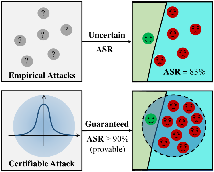
Figure 1: Empirical Attack vs. Certifiable Attack

Certifiable Attacks. As shown in Figure 1, the proposed certifiable attack ensures provable guarantee (certification) for the attack success rate (ASR) of the crafted adversarial examples (e.g., $90\%+$ ASR). Such certifiable ASR can be pre-determined by the adversary as a parameter setting to craft successful adversarial examples with confidence. On the contrary, existing black-box attacks iteratively improve the adversarial perturbations with empirical methods, and the attack success rate (ASR) is completely uncertain before performing the prediction on the adversarial example by the target model (also see Figure 1).

To pursue certifiable attacks, we theoretically bound the attack success rate of adversarial examples based on a novel way of revised randomized smoothing (RS) [12], which has recently achieved great success in certified adversarial robustness. In traditional RS for certified robustness, adding noises $\epsilon$ drawn from predefined distributions $\mu$ to the inputs $x$ turns the standard classifier $f$ into a smoothed classifier $g$. The smoothed classifier outputs the most probable class over the noisy inputs, i.e., $g(x)=\arg\max_{y\in\mathcal{Y}}\mathbb{P}(f(x+\epsilon)=y)$, where $y$ denotes the label of $x$. Given a clean input $x_{0}$ and the smoothed classifier $g$, RS can derive a certified radius $R$ to bound the $\ell_{p}$-norm of perturbations, and guarantee that any perturbation within this certified radius will not fool the smoothed classifier. In other words, for all adversarial examples $x^{\prime}$, if $\|x^{\prime}-x_{0}\|\leq R$, RS can ensure $g(x^{\prime})=g(x_{0})$.

Hiccups of Randomized Smoothing for Certified Defense. Although RS-based certified robustness can certify any arbitrary classifier with a tight bound (e.g., [12]), the setting of such certified defense has certain limitations in practice. Specifically, to determine whether an adversarial example $x^{\prime}$ can trigger the misclassification on the smoothed classifier, RS needs a certification on its clean version $x_{0}$ to compute the certified radius. However, in real-world scenarios, the defender (aka. model owner) usually only receives the adversarial example $x^{\prime}$ before the classification and may not have access to the corresponding clean version $x_{0}$. Therefore, RS-based certification may not be an ideal solution for practical defense due to possibly limited access to the clean inputs.

RS for Certifiable Attacks. Instead, we inversely revise the RS for practical certifiable attacks, which naturally follow the standard threat model of black-box attacks (since the input data can be accessed and manipulated by the adversary). Specifically, we establish an RS-based certifiable attack framework that can craft probabilistic adversarial examples (PAE) with provable guarantees to the lower bound of the attack success rate. The PAEs are random variables in the input space following a specific probabilistic density function (PDF) and the ASR of the PAEs can be guaranteed by our method.

The goal for the RS-based certifiable attack is intuitive, i.e., can we guarantee the outputs of classifier are consistently wrong? However, a series of new significant challenges should be addressed in the design.

1. Existing randomized smoothing theory (for defenses) cannot be directly generalized to certifiable attacks.

2. The target classifier that the adversary has access to is a standard classifier rather than the smoothed classifier.

3. How to efficiently craft the adversarial examples that can ensure wrong predictions is challenging.

4. How to make the probabilistic adversarial examples as imperceptible as possible is also challenging.

To tackle these new challenges, in this paper, we make the following significant contributions: 1) proposing a novel certifiable attack theory based on randomized smoothing, which can universally guarantee the adversarial success rate (ASR) of probabilistic adversarial examples (PAEs) using different noise distributions; 2) designing a randomized querying method that can consider any arbitrary target classifier as a smoothed classifier in the black-box setting (without knowing the target model); 3) proposing a novel self-supervised initialization method to efficiently generate successful PAEs; 4) designing a novel geometric shifting method to reduce the perturbation size while maintaining the guarantee for the attack. Note that the proposed certifiable attack can leverage any continuous noise distribution, e.g., Gaussian, Laplace, and Cauthy distributions, to craft the PAEs.

Furthermore, certifiable attack studies a new direction of adversarial attacks, and aims to raise new vulnerabilities of machine learning models. Therefore, to measure these risks, we thoroughly evaluate the performance of the proposed certifiable attack under many different settings on multiple datasets. We also discuss and evaluate the performance of the certifiable attack against multiple defense methods including the existing general defenses and possible adaptive defenses.

2 Related Work

Adversarial Evasion Attack. Adversarial evasion attacks aim to trigger the misclassification in machine learning models by perturbing the inputs with malicious but imperceptible noises. The adversarial evasion attacks can be divided into two main categories, i.e., white-box attacks [18, 34, 8, 32, 51] and black-box attacks [5, 10, 23, 9], according to the access that the adversary holds. In the white-box setting, adversaries have the full access to the model parameters and the model outputs, while in the black-box setting, adversaries only have the access to the outputs of the models (either the prediction scores or the prediction labels). It is widely believed that the black-box attack has more practical settings for the real world scenarios [37, 4, 9]. Therefore, we focus on the black-box attacks in this paper.

Black-box Attacks. The black-box attacks can be classified into three types according to how they are crafted: by gradient estimation, by transferring from surrogate models, or by locally searching. Many works [10, 22, 11, 3, 15] leverage the gradient of the loss function w.r.t. the inputs to guide the adversarial example generation since the gradient contains important information on how much the pixel changes can affect the prediction loss function. However, in the black-box setting, it is hard to obtain the real gradients since the adversary have no access to the model parameters. Therefore, these adversaries tend to rely on estimating the gradients. Another line of works [37, 44, 14, 35] focus on combining surrogate models and the white-box attacks to generate adversarial examples since the white-box attacks have achieved great success to craft malicious examples. The challenge in these works is to ensure the transferability of the adversarial example from the surrogate models to target models. Many other works [5, 6, 29, 20, 1] focus on crafting the adversarial examples by searching the malicious perturbations. For example, SimBA [20] iteratively find the best direction to update the perturbation, and Boundary Attack [5] traverses the decision boundary to craft the least imperceptible perturbations. All the existing black-box attacks rely on empirical strategies to attack the target model, although most of them have high attack success rate (ASR), and some of them even have $100\%$ ASR. Without the limitation to the query, these empirical attacks can query the target model for numerous times until if finds a successful adversarial example. However, none of them can ensure the attack success before querying the target model with the latest version of the adversarial example and receiving a wrong prediction result.

Empirical Defense. Empirical Defenses aim to empirically defend against the adversarial attacks. Although there is no guarantee to the defense, empirical defenses are efficient to tackle the attacks especially when the defense is designed for targeting certain types of attacks. The empirical defense can be categorized into four classes. The gradient-masking defenses [36, 52, 13] modify the model inference process to obstacle the gradient computation. The input-transformation defenses [19, 7, 42, 30, 45] use pre-processing methods to transform the inputs so that the malicious effects caused by the perturbations can be reduced. One of the important empirical defenses is the adversarial training [32, 43, 49, 48]. By incorporating adversarial examples in the training data, the adversarial training aims to train a more robust model that can resist the malicious inputs. There is also a track of works [40, 47, 31, 33, 24] focusing on detecting the adversarial examples as a defense.

Certified Defense. Certified defense [25, 17, 2, 50] was proposed to guarantee constant prediction for a classifier when adversarial examples are within a neighboring area of the input. Recently, randomized smoothing [12] has achieved great success in the certified defense since it is the first method that can certify arbitrary classifiers of any scales. Specifically, randomized smoothing can guarantee the prediction if the perturbation is bounded by a distance in $\ell_{p}$-norm, i.e., certified radius. Given any input $x$, a corresponding certified radius can be computed using existing randomized smoothing methods [12, 46, 55]. However, the certified defense is not practical in the real-world scenarios. First, certified defense cannot protect unknown inputs due to the certification can be unavailable in the real-world setting. Given an adversarial input, if its clean version of input has not been certified, the certified radius for the clean input is not available and model owner cannot know whether the adversarial example is within the certified radius or not. Even if the attack is performed on the clean images that have been certified beforehand, given the adversarial example, the model owner may not recognize its corresponding clean version. Second, the certification may be performed on adversarial examples. If the certification is performed on a successful adversarial example, certified defense will guarantee the prediction is constantly wrong. In this way, the certified defense technique can be utilized by the adversaries to protect their well-crafted adversarial examples. In this paper, we leverage the randomized smoothing to protect our crafted adversarial examples.

3 Certifiable Black-box Attack

3.1 Threat Model

We first define the threat model of the certifiable attack. To further evaluate the certifiable attack’s performance in reality, we also consider more challenging situations (for the attack) when the model is protected by different levels of defenses. Thus, the threat model can be defined as follows:

• Adversary: The adversary aims to craft adversarial example(s) and guarantee the attack success rate (ASR) on it before the attack. Similar to the traditional black-box attacks [8, 9], the adversary can modify the input data in the inference stage, and has the query access to the hard-label outputs of the target model while generating the adversarial perturbation. However, we assume that the adversary does not need the query access to the final version of the adversarial example since the attack success rate (ASR) should be guaranteed before the attack.

• Model Owner: The model owner aims to pursue correct prediction for its model. In this paper, we consider three different levels of the ML model’s knowledge and capability: 1) The model has no awareness of the adversarial attacks, and is not equipped with any defense; 2) The model owner is aware of the adversarial attack, but has no knowledge of the attack method. The model owner is able to deploy some general defense methods; 3) The model owner is aware of the adversarial attack, and has knowledge about the attack method. The model owner is able to deploy some adaptive defenses.

The certifiable attack considers a novel scenario that has never been explored, which may reveal new risks for machine learning systems. For example, say there is a machine learning-based system (e.g., auto-driving, auto-diagnosis, or surveillance system). The adversary would like to subvert these systems via the adversarial examples (AEs) over the ML models. If using the traditional black-box attack, the adversary needs to repeatedly query the system until the final crafted AE causes misclassification. In practical systems, all the queries and the final AEs are very likely to be logged by the system, e.g., for auditing, anomaly detection, and security vulnerability analysis. The system can simply block the adversary’s AE and previous inputs in the queries (e.g., creating a blacklist for AEs) after the logging, auditing, or analysis.

Specifically, in autonomous driving and surveillance scenarios, attackers may need to continuously attack the model with the same data (e.g., image/video frames at the same scene), then traditional black-box attacks (with the same AE) would not be able to succeed anymore unless the adversary crafts a completely new AE with a series of new queries. In certifiable attacks, the certified adversarial example is re-usable (does not need queries anymore) and can generate various unseen AEs, which cannot be simply blocked either (since many of them are actually not very similar due to noise injection). Such unseen AEs (new to the system) with guaranteed success rates can be generated at any time without re-quering the system. This would be an additional benefit for the adversary since the adversary can opt to only perform highly-confident attacks while reducing the interaction (queries) over the target model or system.

3.2 Certifiable Adversarial Success Rate

Considering a classification problem from $\mathbb{R}^{d}$ to classes $\mathcal{Y}$. Given a clean input $x_{o}\in\mathbb{R}^{d}$ and its label $y\in\mathcal{Y}$. We can find an adversarial example $x$, and then craft the probabilistic adversarial examples (PAE) by adding perturbations $\delta\in\mathbb{R}^{d}$ and noise $\epsilon\in\mathbb{R}^{d}$ drawn from a distribution $\mu$ to the adversarial example $x$:

$$x_{adv}=Clip\{x+\delta+\epsilon\}$$ (1)

where the $Clip\{\cdot\}$ denotes the clip operation which clips the pixel value of the adversarial example to a range (e.g., $[0,255]$) since PAE may have probabilistic pixel values out of the range. Any sample of the PAE is a standard adversarial example, and the attack success rate of the samples can be lower-bounded by a threshold $p$:

$$\mathbb{P}(f(x_{adv})\neq y)\geq p$$ (2)

where the value of constant $p$ is defined as the certifiable attack success rate (CASR).

3.3 Randomized Query

Different from the randomized smoothing in certified defense, the smoothed classifier is not available to the adversary. In the certified defense, the smoothed classifier is constructed by adding the noise to the input and calculate the predictions over the noise. From the perspective of attacks, since the adversary has the query access to the target model, the adversary can also turn any arbitrary classifier into a “smoothed classifier” by injecting the noise into the input and querying the prediction results (the classifier can be considered as a randomly smoothed classifier w.r.t. the noisy queries). Specifically, for any input pair $(x,y)$, any target classifier $f:\mathbb{R}^{d}\rightarrow\mathcal{Y}$, and the noise $\epsilon$, the adversary can perform the randomized query:

$$Q(x)=\mathbb{P}(f(Clip\{x+\epsilon\})\neq y)$$ (3)

By this definition, the randomized query will return the probability of the incorrect prediction over the noise. Note that, the clip operation is necessary after the noise injection since the adversary example should follow the image formation. Although this operation will clip the noise distribution, it will not affect the guarantee since we can consider a new classifier $f^{\prime}(\cdot)\equiv f(Clip\{\cdot\})$, and certify this new classifier. For simplicity of notations, we skip $Clip\{\cdot\}$ in the notations in the rest of the paper (by considering it as the default setting). Moreover, in the certified defense, the smoothed classifier is usually trained on the noise-perturbed data to improve the classification performance. Although in the certifiable attack, the target model is a standard classifier trained on the data without noise, high certification accuracy for certifiable attack can be easily achieved (see Section 5 for the experimental results) since the false classes are the majority out of all the classes.

The certifiable attack is designed based on the randomized query (one-time). Once the randomized query satisfies some conditions, the PAE can be crafted and the success of the attack can be guaranteed with provable confidence. We will propose the theory to craft the PAE and guarantee the attack success in Section 3.4.

3.4 Certification Theory

In this section, we propose the theory that guarantees the attack success rate of the PAE if the randomized query satisfies some conditions. The certification starts from finding a standard adversarial example $x$ such that the lower bound of the randomized query is larger than the pre-defined CASR $p$, then we construct the PAE as $x_{adv}=x+\delta+\epsilon$, and guarantee the attack success rate of the crafted PAE for all the perturbations $\delta$ computed by our theorem. The theory of certifying a PAE is presented in Theorem 1.

Theorem 1.

(Certifiable Adversarial Attack) Let $f:\mathbb{R}^{d}\rightarrow\mathcal{Y}$ be any deterministic or random function, let $x_{o}$ be any clean input, $y$ be the label of $x_{o}$. Let $x$ be an adversarial example of $x_{o}$, $\delta$ be any perturbation, and $\epsilon$ be the noise drawn from any continuous probability density function (PDF) $\mu$. Let $p$ be the pre-defined certifiable attack success rate (CASR). Denote $\underline{p_{adv}}\in[0,1]$ as the lower bound of the randomized query. If the randomized query on the adversarial input satisfies Eq. (4):

$$Q(x)=\mathbb{P}(f(x+\epsilon)\neq y)\geq\underline{p_{adv}}\geq p$$ (4)

Then, the probabilistic adversarial example $x_{adv}\equiv x+\delta+\epsilon$ is guaranteed to have certifiable attack success rate $p$ if the perturbation $\delta$ satisfies:

$$\Phi_{+}(\Phi_{-}^{-1}(\underline{p_{adv}}))\geq p$$ (5)

where $\Phi_{-}^{-1}$ denotes the inverse cumulative density function (CDF) of the random variable $\frac{\mu(\epsilon-\delta)}{\mu(\epsilon)}$, and $\Phi_{+}$ denotes the CDF of the random variable $\frac{\mu(\epsilon)}{\mu(\epsilon+\delta)}$.

Proof.

See the Appendix A for the proof. ∎

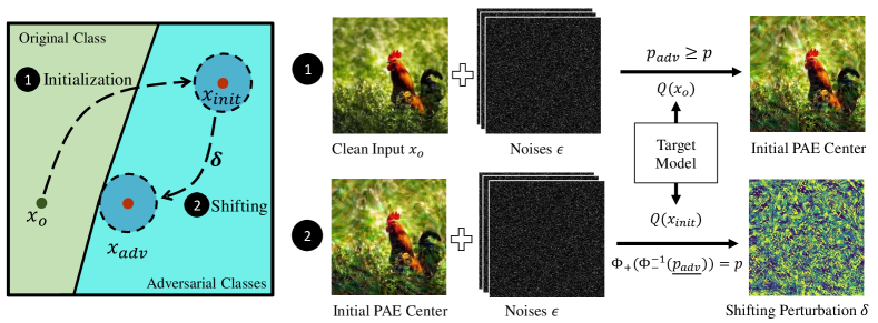
Figure 2: Overview of Crafting Certifiable Adversarial Example

Theorem 1 guarantees the PAE’s attack success rate if the conditions Eq. (4) and Eq. (5) hold. The satisfaction of condition Eq. (4) is equivalent to the certification of PAE (once the condition Eq. (4) is satisfied at least we can find $\delta=\textbf{0}$ to satisfy condition Eq. (5)). Therefore, finding a proper $x$ to satisfy condition Eq.(4) can craft an initial successful PAE $x_{adv}=x+\epsilon$. The satisfaction of condition Eq. 5 allows the adversary to further craft more optimal PAE by finding proper $\delta$. For example, under the constrain of condition Eq. (5), we can find a perturbation $\delta$ towards the clean input to reduce the distance between the PAE and the clean input, which can increase the imperceptibility of the PAE. In conclusion, these two conditions formalize two important problems in crafting the PAE: the initialization (see Section 4.1) and the certifiable attack shifting (see Section 4.2).

We also present a special case of Theorem 1 when the noise is Gaussian in Corollary 1.2 in Appendix B. It shows that to guarantee the certifiable attack, the perturbation $\delta$ should satisfies $||\delta||_{2}\leq\sigma(\Phi^{-1}(p_{adv})-\Phi^{-1}(p))$, where $\Phi^{-1}$ denotes the inverse of Gaussian CDF.

4 Attack Design and Analysis

In this section, we design the certifiable attack and give corresponding theoretical analysis. Specifically, we craft the PAE by finding a successful initial PAE with strictly satisfied condition Eq. 4 (see the step ① in Figure 2), and then shifting the PAE towards the clean input for reducing the perturbation size (better imperceptibility) while maintaining the guarantee (see the step ② in Figure 2).

4.1 Initialization

The initialization aims to find an input to satisfy the condition Eq. (4), which determines whether the PAE can be certified. The simplest initialization is the random initialization, where the input $x$ is uniformly sampled from the input space $[0,\ 255]^{d}$, followed by a randomized query to check if the $\underline{p_{adv}}$ is larger than the CASR. However, the random initialization may not generate the optimal initial adversarial examples due to the intractable stochastic process, and the perturbation could be very large. To efficiently find a more optimal initial PAE, we leverage the self-supervised perturbation (SSP) [35] to design a novel initialization method for the certifiable attack, namely smoothed self-supervised perturbation (SSSP). The SSP attack generates generic adversarial examples that distort the features extracted by a general feature extractor (pre-trained on ImageNet [41]) in a self-supervised manner. Since the certifiable attack is designed based on the randomized queries, we alternatively generate the adversarial example that distorts the features extracted from the noise-perturbed inputs. Specifically, The goal of the proposed SSSP initialization can be described in the following Equation:

$$\max_{\delta}||\mathcal{F}(x_{o}+\delta+\epsilon)-\mathcal{F}(x_{o}+\epsilon)||_{2}$$ (6)

where $\mathcal{F}$ denotes the feature extractor, $x_{o}$ denotes the clean image, and $||\cdot||_{2}$ denotes the $\ell_{2}$-norm distance. By solving this optimization problem, we can find a perturbation that distorts the features of all the noise-perturbed inputs, which makes the randomized query more likely to return a false class since the randomized query also rely on the noise-perturbed inputs. Note that the feature extractor is pre-trained on large-scale dataset and the features can be transferred to other classifiers, so the proposed SSSP initialization can be generalized to various classifiers to efficiently find the initial PAE.

To solve this optimization problem, we leverage the Projected Gradient Descent method [32] to update the PAE in an offline manner. Let the adversarial loss $\mathcal{L}(x)\equiv\mathbb{E}_{\epsilon\sim\mu}[||\mathcal{F}(x+\delta+\epsilon)-\mathcal{F}(x+\epsilon)||_{2}]$. Then the PAE can be initialized by iteratively perturbing it along the direction of gradient ascending:

$$x_{init}^{t+1}=x_{init}^{t}+c\ sgn(\nabla_{x_{init}^{t}}\mathcal{L})$$ (7)

where $x_{init}^{t}$ denotes the center of current initial PAE, $x_{init}^{t+1}$ denotes the updated center of initial PAE, $sgn(\cdot)$ denotes the sign function, and $c$ denotes the step size for updating the PAE. Now we know how to update the PAE towards a promising direction that can satisfy the certification condition. However, the size of perturbation can be a problem. On one hand, larger perturbations tend to craft successful PAE due to large distortion, but it will make the input more perceptible. On the other hand, small perturbations are more imperceptible, but may not successfully fool the classifier. Therefore, we initialize the PAE by updating the PAE from a small perturbation to a large perturbation, and perform the randomized query in each iteration of the updating. The details for the PAE initialization are summarized in Algorithm 1 and 2. The comparison of the random initialization and the SSSP initialization can be found in Section 5.1.4.

Algorithm 1 SSSP Initialization

1:The clean input $x$, the feature extractor $\mathcal{F}(\cdot)$, the randomized query function $Q(\cdot)$, the smoothed self-supervised perturbation algorithm $SSSP(\cdot)$ (Algorithm 2), the initial perturbation size $\Gamma_{init}$, the perturbation size increasing step $\gamma$, the certifiable attack success rate $p$, the initialization maximum number of iterations $N_{max}$, and the noise distribution $\mu$.

2:The center of initial probabilistic adversarial example $x_{init}$, the number of queries $q$

3:$x_{init}=SSSP(x,\ \mathcal{F},\ \Gamma_{init})$

4:$\Gamma=\Gamma_{init}$, $N=0$, $q=0$

5:while $Q(x_{init})<p$ and $N<N_{max}$ do

6:     $N=N+1$

7:     $q=q+1$

8:     $\Gamma=\Gamma+\gamma$

9:     $x_{init}=SSSP(x_{init},\ \mathcal{F},\ \Gamma)$

10:end while

11:if $Q(x_{init})<p$ then

12:     return Abstain

13:else

14:     return $x_{init}$ and $q$

15:end if

Algorithm 2 Smoothed Self-supervised Perturbation (SSSP)

1:The PAE center $x_{c}$, the clean input $x$, the feature extractor $\mathcal{F}$, the loss function $\mathcal{L}$, the noise distribution $\mu$, the maximum number of updating iteration $n_{max}$, the perturbation size $\Gamma$, the updating step size $c$.

2:The center of probabilistic adversarial example $x^{\prime}$

3:for $n=1$ to $n_{max}$  do

4:     $\delta=c\ sgn(\nabla_{x_{c}}\mathcal{L}(\mathcal{F}(x_{c}+\epsilon),\mathcal{F}(x+\epsilon))),\ \epsilon\sim\mu$

5:     $x_{c}=x_{c}+\delta$

6:     $x_{c}=Clip(x_{c},\ x-\Gamma,\ x+\Gamma)$

7:     $x_{c}=Clip(x_{c},\ 0.0,\ 1.0)$

8:end for

9:return $x^{\prime}$

4.2 Certifiable Attack Shifting

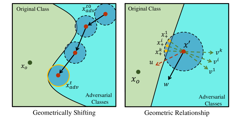
Figure 3: Certifiable Attack Shifting

The certifiable attack shifting aims to reduce the perturbation size of PAE while maintaining the certifiable attack guarantee. The initialization crafts an initial PAE, but the imperceptibility of the PAE is still not optimal. In the classification problem, the optimal imperceptibility can be achieved when the PAE is close to the decision boundary. Therefore, we can shift the PAE towards the clean input to reduce the size of the perturbation until intersecting the decision boundary, namely “certifiable attack shifting”. Note that the PAE can be crafted by any $\delta$ with the satisfaction of Eq. 5, we can shift the PAE from the initial PAE towards the clean input with the maximum $\delta$ without breaking the guarantee. By iteratively executing the randomized query and applying the Theorem 1, the PAE can be repeatedly shifted until the decision boundary is approached. As the Corollary 1.1 states, the center of the previous PAE naturally satisfies the condition Eq. (4). Then, a new PAE can be crafted using the Theorem 1. According to the Corollary 1.1, although we know that $Q(x+\delta)\geq p$, we still need to run the randomized query to obtain the lower bound $p_{adv}$ in order to derive the new $\delta$.

Corollary 1.1.

(Certifiable Attack Shifting) If a probabilistic adversarial example $x_{adv}\equiv x+\delta+\epsilon$ is certifiable, then the center $x+\delta$ also satisfies Condition Eq. (4).

Proof.

If a PAE is certifiable, then according to Theorem 1, the attack success rate of $x_{adv}$ is at least $p$. Thus, we have $\mathbb{P}(f(x_{adv})\neq y)=\mathbb{P}(f(x+\delta+\epsilon)\neq y)=Q(x+\delta)\geq p$. ∎

Now we can shift the PAE to reduce the perturbation size without degrading the provable guarantee, another important but unaddressed problem is how to determine the $\delta$ to shift the PAE. We design a novel shifting method to find the locally-optimal PAE by considering the geometric relationship between the decision boundary and the PAE, which is called “Geometrically Shifting”. Specifically, through using the noisy samples of PAE to “probe” the decision boundary, we shift the PAE along the decision boundary and towards the clean input until finding the local optimal point on the decision boundary (also see Figure 3 for the illustration). If none of the noisy samples can approach the decision boundary, we simply shift the PAEs directly towards the clean input without considering the decision boundary.

A major challenge is to find the direction along the decision boundary when the PAE approaches the decision boundary. The geometrical relationship is presented in the right side of Figure 3. The first step is to find the shifting direction to shift along the decision boundary. The second step is to determine the shifting distance which maintains the guarantee. Denote $x^{\prime}$ as the center of the current PAE. When sampling the adversarial examples from the PAE, we mark the failed adversarial examples as $x^{1}_{+},x^{2}_{+},...,x^{i}_{+},...,x^{k}_{+}$, aka “samples fell into the original class”. The unit vector points from $x_{+}^{i}$ to $x^{\prime}$ is denoted as $v^{i}$. The unit vector points from $x^{\prime}$ to $x_{o}$ is denoted as $u$. If the PAE has no samples crossing the decision boundary, then we can shift the PAE straightly towards the clean input (along the direction of $u$) until it intersects the decision boundary. If there are some failed samples $x^{i}_{+}$, we know where the decision boundary is, and the shifting should be parallel to the decision boundary (without changing the certifiable attack guarantee). Note that the input space is high-dimensional, thus there could be many directions parallel to the decision boundary. To reduce the perturbation size, the direction should be similar to the vector $u$ as much as possible. Based on these geometric analyses, the goals of the geometrically shifting can be summarized as:

• The shifting direction should be parallel to the direction of $u$; and be vertical to the vectors $v^{i}$.

Denoting the shifting direction as $w$, if use the cosine similarity to measure the direction similarity, then the goal of finding the shifting direction can be expressed as:

$$w=\arg\max\sum_{i=1}^{k}sin(v^{i},w)+cos(u,w)$$ (8)

where $sin(\cdot)$ and $cos(\cdot)$ denote the sine and cosine similarity of two vectors, respectively. The shifting direction can be found by solving the Eq. (8) and the shifting distance can be determined by finding the maximum $||\delta||_{2}$ with the constraint of Eq. (5), which guarantees the certifiable attack. We leverage the gradient descent algorithm to solve Eq. (8) and binary search to find the maximum $||\delta||_{2}$. Specifically, the maximum $||\delta||_{2}$ can be achieved when the equality in Eq. (5) holds, then we use binary search to approach the equality with the constraint of Eq. (5). The algorithm for finding the shifting direction and distance are presented in Algorithm 3 and Algorithm 4, respectively. Similar to [21], we use the Monte Carlo method to estimate the CDF of random variable $\frac{\mu(\epsilon-\delta)}{\mu(\epsilon)}$ and $\frac{\mu(\epsilon)}{\mu(\epsilon+\delta)}$. To estimate the lower bound of the probability, we follow [12] to compute the one-side lower confidence interval for the Binomial test.

Provable Guarantee of Shifting. Note that any $\delta$ computed by the Algorithm 4 will not violate the certifiable attack guarantee since it ensures $\Phi_{+}(\Phi^{-1}_{-}(\underline{p_{adv}}))\geq p$, even when the shifting direction is not parallel to the decision boundary. For example, when the shifting direction is orthogonal to the decision boundary, the computed $\delta$ will be very small so the PAE will not cross the decision boundary. When the shifting direction is parallel to the decision boundary, the computed $\delta$ can be large. In this way, the geometrically shifting is more likely to find a local optimal PAE by moving along the decision boundary. Provable ASR can still be ensured in all these shifting cases.

Algorithm 3 Shifting Direction

1:The center of the PAE $x_{c}$, the clean input x, the vectors $\{v^{i}\}$, the vector $u$, the maximum number of iterations $M$, the updating step size $c^{\prime}$.

2:The shifting direction $w$

3:# Initialize $w$ with random noise

4:if  $\{v^{i}\}$ is empty then

5:     $w=x-x_{c}$

6:else

7:     $w=rand(\mathbb{R}^{d})$

8:     for $j=1$ to $M$ do

9:         $w=w+c^{\prime}sgn(\nabla_{w}({\sum_{i=1}^{k}sin(v^{i},w)+cos(u,w)}))$

10:         $w=\frac{w}{||w||_{2}}$

11:     end for

12:end if

13:return $w$

Algorithm 4 Shifting Distance

1:The center of PAE $x_{c}$, the noise distribution $\mu$, the number of Monte Carlo samples $N_{m}$, the confidence $1-\alpha_{o}$, the randomized query function $Q(\cdot)$, the lower bound function $LOWERBOUND(\cdot)$, the shifting direction algorithm $SD(\cdot)$ (Algorithm 3), error threshold $e$, the certifiable attack success rate $p$, the maximum number of iterations $M^{\prime}$.

2:The shifting perturbation $\delta$

3:$w=SD(x_{c})$

4:$p_{adv}=LOWERBOUND(Q(x_{c}),1-\alpha_{o},N_{m})$

5:find constant $a$ such that $\delta=aw$ and $\Phi_{+}(\Phi_{-}^{-1}(\underline{p_{adv}}))>p$

6:find constant $b$ such that $\delta=bw$ and $\Phi_{+}(\Phi_{-}^{-1}(\underline{p_{adv}}))<p$

7:$\delta=\frac{(a+b)}{2}w$

8:$m=0$

9:while $\Phi_{+}(\Phi_{-}^{-1}(\underline{p_{adv}}))<p$ or $>p+e$ and $m<M^{\prime}$ do

10:     if $\Phi_{+}(\Phi_{-}^{-1}(\underline{p_{adv}}))>p$ then

11:         $a=\frac{(a+b)}{2}$

12:     else

13:         $b=\frac{(a+b)}{2}$

14:     end if

15:     $\delta=\frac{(a+b)}{2}w$

16:     $m=m+1$

17:end while

18:if $m=M^{\prime}$ then

19:     return Abstain

20:else

21:     return $\delta$

22:end if

4.3 Theoretical Analysis

In this section, we analyze the convergence of the algorithms and the confidence bound. With the centralized noise distribution, the shifting algorithm is guaranteed to converge once the initial PAE is found. We show this theoretical guarantee in Proposition 1.

Proposition 1.

If the noise distribution $\mu(x)$ decreases as the $|x|$ increases, with the satisfaction of Condition Eq. 4, given any vector direction $w$, the binary search algorithm is guaranteed to find the $\delta$ such that $\Phi_{+}(\Phi_{-}^{-1}(\underline{p_{adv}}))=p$ with confidence $(1-\alpha_{o})(1-2e^{-2N_{m}\Delta^{2}})^{2}$, where $(1-\alpha_{o})$ is the confidence for the $\underline{p_{adv}}$ estimation, $N_{m}$ is the number of Monte Carlo samples, and $\Delta$ is the error bound for the CDF estimation.

Proof.

See detailed proof in Appendix C. ∎

5 Experimental Evaluations

In this section, we comprehensively evaluate the performance of the certifiable black-box attack in different circumstances with various settings. Specifically, we evaluate the performance of the proposed certifiable attack on the models without defense method in Section 5.1. In Section 5.2, we evaluate the performance of the certifiable attack when some general defenses (e.g., adversarial training [32], adversarial example detection [54], and certifiable defense [12]) are deployed. In Section 5.3, we evaluate the proposed certifiable attack in more challenging circumstances (from the perspective of attacks), where adaptive defenses are deployed before the certification. Certifiable attack is a new direction which is different from the empirical attacks. Due to different attack objectives and settings, it is unfair to compare the attack performance (e.g., success rates) of certifiable and empirical methods (lack of provable guarantees for the ASR). Therefore, we compare them based on implementing the attack (e.g., runtime).

Datasets. We evaluate the certifiable attack on two popular datasets for image classification: CIFAR10 [27] and ImageNet [41]. CIFAR10 is a small-scale dataset with $10$ classes. The training set has $60,000$ images and the test set has $10,000$ images. Each image has the dimension $3\times 32\times 32$. ImageNet is a large-scale datset with $1,000$ classes. The training set contains $1,281,167$ images and the validation set contains $50,000$ images. The image in ImageNet is resized to $3\times 224\times 224$ for training and inference. In this paper, we train the models on the entire training set for each dataset, and evaluate the performance on the entire test set for CIFAR10 and on $500$ samples of the validation set for ImageNet.

Metrics. Several metrics are used for evaluating the certifiable attack: the certification accuracy, the average $\ell_{2}$-distance, and the number of randomized queries. The certification accuracy is the percentage of the test samples that have the certifiable PAE, which is also the ratio of the successful initialization over all the test samples. Since the PAE is a noise distribution, to evaluate the perturbation size, we average the $\ell_{2}$-norm of the perturbation drawn from the PAE (see Eq. (9)). Each randomized query contains a set of parallel queries, and different adversaries may have different setting for the number of parallel queries, so we evaluate the certifiable attack by deriving the number of randomized queries for fair comparison.

$$Ave\_dis=\mathbb{E}_{\epsilon\sim\mu}(||x+\delta+\epsilon-x_{o}||_{2})$$ (9)

Experimental Settings. In all the experiments, we adopt $N_{m}=1,000$ as the number of Monte Carlo samples, $\alpha_{o}=0.001$ as the lower bound estimation, and $1,000$ as the batch size. For the initialization, we set $N_{max}=85$ as the maximum number of iterations, $\Gamma_{init}=3/255$ as the initial perturbation size, and $\gamma=3/255$ as the perturbation size increasing step. For the shifting, we set $M^{\prime}=72$ as the maximum number of iterations, $\alpha_{o}=0.001$ as the confidence, and $e=0.01$ as the error threshold. If not specify, we use Gaussian noise with $\sigma=0.25$ as the noise distribution, and set the CASR as $p=90\%$.

Experimental Environment. All the experiments were performed on the NSF Chameleon Cluster [26] with Intel(R) Xeon(R) Platinum 8380 CPU @ $2.30$GHz CPUs, $512$G RAM, and NVIDIA A100 PCIe $80$GB GPUs.

5.1 Certifiable Adversarial Attack

We first evaluate the performance of the certifiable attack on models without defense methods. Specifically, we evaluate the performance of certifiable attack under different settings, e.g., different noise variances, different CASRs, and different noise distributions. We also evaluate the certifiable attack using different initialization and shifting methods.

5.1.1 Performance on Different Noise Variances

We first present the performance of the certifiable attack using different variances to generate noise for the images. The results are presented in Table 1. On both CIFAR10 and ImageNet, we observe that as the variance increases, the average $\ell_{2}$-distance increases. This is because given larger noise variances, the adversarial examples tend to cover a larger area in the input space. Since certifiable attack requires that $p\%$ of the adversarial samples fall into the false classes, the center of the PAE will be far from the decision boundary. Figure 4 also gives such insight. We can also observe that as the variance increases, the number of randomized queries decreases. This is because that the larger variance usually leads to a larger shifting step. It takes fewer steps to move to the decision boundary when the variance increases. Finally, we observe that the certified accuracy on the CIFAR10 decreases as the variance increases. The certified accuracy has already been determined in the initialization. Larger certified accuracy means that it is easier to find the PAE. Hence, the results on CIFAR10 show that it is easier to find a small area of adversarial examples than a large area of adversarial examples. On the ImageNet, it is easy to find the adversarial examples for both large and small noise scales (since $999$ out of $1,000$ classes are all false classes). Thus, the certified accuracy is nearly $100\%$.

	$\sigma$	Ave. $\ell_{2}$-dis.	Rand. Query	Certified Acc.
CIFAR10	0.10	7.39	18.34	94.17%
	0.25	12.95	14.35	91.21%
	0.50	19.41	11.38	90.00%
ImageNet	0.10	41.80	32.55	99.80%
	0.25	87.47	17.02	99.60%
	0.50	135.47	8.31	100.00%

Table 1: Performance of Certifiable Black-box Attack with Gaussian Noise. The CASR threshold is set as $p=90\%$, and the $\sigma$ denotes the standard deviation of the noise.

5.1.2 Performance on Different CASR Thresholds

We also study the relationship between the performance of certifiable attack and the CASR threshold. As Table 2 shows, on both CIFAR10 and the ImageNet datasets, as $p$ increases, both the average $\ell_{2}$-distance and the number of the randomized queries increases. We also illustrate the reasons for this observation in Figure 4. On one hand, a larger $p$ means that it requires more adversarial examples falling into the false classes. When the noise variance is fixed, the center of the PAE should be further away from the decision boundary to allow more adversarial samples falling into the false classes. On the other hand, the smaller $p$ will lead to a larger shifting step since the shifting step depends on the gap between the CASR $p$ and the lower bound of the probability returned by the randomized query $\underline{p_{adv}}$ (see the Gaussian-case of Theorem 1 in Appendix B). With a larger shifting step, the required number of randomized queries can be fewer. We also observe that smaller $p$ results in a higher certified accuracy on CIFAR10 since smaller $p$ could allow more failed adversarial samples. This will make the initialization easier. On ImageNet, the initialization is easy no matter how the CASR threshold changes.

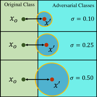
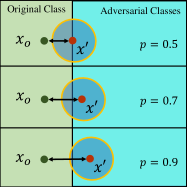
Figure 4: Illustration of the Experimental Results with Different Noise Variances (left) and CASR Thresholds (right)

	p	Ave. $\ell_{2}$-dis.	Rand. Query	Certified Acc.
CIFAR10	50%	12.65	9.34	97.17%
	60%	12.72	11.09	95.85%
	70%	12.80	11.94	94.72%
	80%	12.87	12.37	93.17%
	90%	12.95	14.35	91.21%
	95%	13.09	15.93	90.37%
ImageNet	50%	85.88	12.85	100.00%
	60%	86.20	13.63	100.00%
	70%	86.45	14.33	100.00%
	80%	87.03	16.02	100.00%
	90%	87.47	17.02	99.60%
	95%	88.42	19.81	100.00%

Table 2: Performance of Certifiable Black-box Attack with Gaussian noise and standard deviation $\sigma=0.25$.

5.1.3 Performance on Different Noise Distributions

Our attack can use any continuous noise distribution to craft the PAE. In this section, we evaluate the performance of certifiable attack using different noise distribution. Specifically, we select Cauthy distribution, Hyperbolic Secant distribution, and the general normal distributions as the candidates. We evaluate the certifiable attack with different noise distributions by adjusting the distribution parameters to ensure consistent variances for fair comparison.

The results are presented in Table 3, and the noise distributions are plotted in Figure 4. We observe that the average $\ell_{2}$-distance is decreasing as the noise distribution is more centralized on both CIFAR10 and ImageNet. In general, the Cauthy distribution is the most centralized distribution, and it provides the smallest average $\ell_{2}$-distance and needs the largest number of randomized queries on both datasets. We conjecture that the centralized distribution lies the adversarial examples close to the center of PAE. Then, the center can be closer to the decision boundary without letting too many samples across the decision boundary. It is hard to say which distribution is better since there is a trade-off between the average $\ell_{2}$-distance and the number of randomized queries.

	Distribution	Density	Ave. $\ell_{2}$-dis.	Rand. Query	Certified Acc.
CIFAR10	Gaussian	$\propto e^{-|x/\alpha|^{2}}$	12.95	14.35	91.21%
	Cauthy	$\propto\frac{\alpha^{2}}{x^{2}+\alpha^{2}}$	7.82	32.77	94.12%
	Hyperbolic Secant	$\propto sech(|x/\alpha|)$	12.51	14.59	91.67%
	General Normal ($\beta=1.5$)	$\propto e^{-|x/\alpha|^{\beta}}$	12.74	14.15	91.39%
	General Normal ($\beta=3.0$)	$\propto e^{-|x/\alpha|^{\beta}}$	13.16	14.15	91.25%
ImageNet	Gaussian	$\propto e^{-|x/\alpha|^{2}}$	87.47	17.02	99.60%
	Cauthy	$\propto\frac{\alpha^{2}}{x^{2}+\alpha^{2}}$	46.18	59.94	99.60%
	Hyperbolic Secant	$\propto sech(|x/\alpha|)$	85.57	20.89	99.80%
	General Normal ($\beta=1.5$)	$\propto e^{-|x/\alpha|^{\beta}}$	86.69	17.58	99.80%
	General Normal ($\beta=3.0$)	$\propto e^{-|x/\alpha|^{\beta}}$	88.51	14.99	100.00%

Table 3: Performance of Certifiable Black-box Attack with Different Noise Distributions. The CASR $p$ is set to be $90\%$. The standard deviation is set to be $0.25$ for all the distributions by adjusting the parameters $\alpha$ and $\beta$.

	Method	Initialization	Shifting	Ave. $\ell_{2}$-dis.	Rand. Query	Certified Acc.
CIFAR10	Baseline A	random	no shifting	22.81	9.50	90.74%
	Baseline B	random	geo. shifting	14.16	64.88	90.00%
	Baseline C	SSSP	no shifting	12.98	12.22	91.30%
	Baseline D	SSSP	geo. shifting	12.95	14.35	91.21%
ImageNet	Baseline A	random	no shifting	164.54	1.00	100.00%
	Baseline B	random	geo. shifting	151.37	74.00	100.00%
	Baseline C	SSSP	no shifting	87.69	5.89	100.00%
	Baseline D	SSSP	geo. shifting	87.47	17.02	99.60%

Table 4: Ablation Study with CASR threshold $p=90\%$. The noise distribution is Gaussian noise with $\sigma=0.25$.

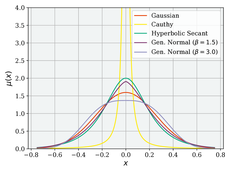
Figure 5: Different Noise Distributions ($\sigma=0.25$)

5.1.4 Ablation Study

We have proposed an initialization method and a shifting method for crafting more optimal PAEs. In this section, we evaluate the performance of our proposed initialization method and the shifting methods by benchmarking with some standard baselines. Specifically, we compare the random initialization and the SSSP initialization. We also compare the geometrically shifting method with none-shifting method. By using different initialization and the shifting methods, we create four baselines (see Baseline A-D in Table 4).

The results are presented in Table 4. We observe that on both CIFAR10 and ImageNet, the SSSP initialization has a much smaller average $\ell_{2}$-distance, and the geometrically shifting also reduces the average $\ell_{2}$-distance. To pursue the insights of how the improvement is achieved, we also present the distributions of the average $\ell_{2}$-distance for each baselines on CIFAR10 in Figure 6. Figure 6 compares the Baseline A and Baseline B, we can see that the geometrically shifting significantly reduces the perturbation sizes by shifting the PAE towards the clean input. By checking the detailed results, we find that most of the PAEs in Baseline A, B, and C have the center exactly on the clean input (the average $\ell_{2}$-distance is around $15$ due to the noise sampling). Therefore, from the results of Baseline A and B, the random initialization initializes the PAEs with large distances (around 25), but the geometrically shifting shifts most of the PAEs back to the clean input. Comparing Baseline A to C, the SSSP can initialize most of the PAEs around the clean input. This is because we adopt an increasing perturbation constraint and the self-supervised perturbation, which can find the “optimal” PAEs closer to the clean input. From the above observation, we see both the SSSP initialization and the geometrically shifting are efficient methods to significantly improve the imperceptibility of PAEs. However, by applying both the SSSP initialization and the geometrically shifting, we only observe a marginal improvement on the average $\ell_{2}$-distance comparing to Baseline C. With the SSSP initialization, the PAEs have already approached the near-optimal positions on the decision boundary, and the geometrically shifting does not need to improve too much.

We also observe that Baseline B has the largest number of randomized queries since it takes many steps to shift the PAE from a random perturbation. With the SSSP initialization, the number of the randomized queries can be significantly reduced since the initial PAE is closer to the clean input. On CIFAR10, we observe that the SSSP initialization can slightly improve the certified accuracy ($1.21\%$).

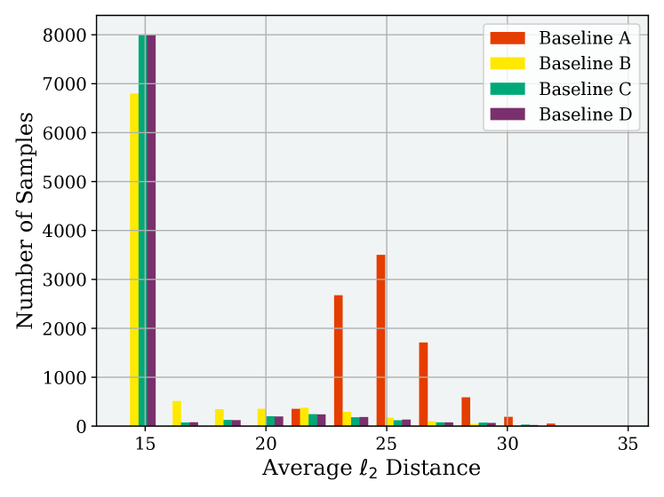
Figure 6: Average $\ell_{2}$-distance Distributions for Different Baselines on CIFAR10

5.2 Performance against General Defenses

We next evaluate the certifiable attack against general defenses. Specifically, we assume that the model owner is aware of the adversarial attack, but do not have detailed information about the attack. Under this assumption, we evaluate the certifiable attack against three different types of the general defenses including the adversarial training, the certified defense, and the adversarial example detection.

5.2.1 Performance against Adversarial Training

The adversarial training is an efficient defense method that trains the classifier with both the clean inputs and adversarial examples. In this way, the model is more resistant to the adversarial inputs while maintaining the performance on the clean inputs. However, the adversarial training usually targets at a specific attack which generates the adversarial examples in the training. To improve the generalizability of the adversarial training, we train the classifier on the self-supervised perturbation attack [35], which is a general attack. Then, we test the certifiable attack to such classifier on CIFAR10. As shown in Table 5, the adversarial training increases the average $\ell_{2}$-distance, the number of randomized queries, and the certified accuracy slightly. This indicates that the adversarial training cannot provide strong defense against our certifiable attacks. Instead, it even improves the certified accuracy slightly.

Defense	Ave. $\ell_{2}$-dis.	Rand. Query	Certified Acc.
No Defense	12.95	14.35	91.21%
AT	13.05	14.58	91.85%
RS	16.11	32.71	88.82%

Table 5: Certifiable Attack against Adversarial Training and Randomized Smoothing ($\sigma=0.25$, $p=90\%$, CIFAR10).

5.2.2 Performance against Randomized Smoothing

The randomized smoothing trains the classifier with noise to improve the performance of the certified defense. We evaluate the certifiable attack on the classifier trained with the same noise. Specifically, we use the Gaussian noise with $\sigma=0.25$ on both the classifier training and the certifiable attack. Table 5 shows that the noise-trained classifier can significantly degrade the performance of certifiable attack. Noticeably, the smoothed training reduces the certified accuracy of the certifiable attack significantly. However, the certifiable attack can still guarantee that $88.82\%$ of the test samples can be provable mis-classified. If we evaluate the randomized smoothing against the certifiable attack (by considering the PAE center as the input), we will find that the certified accuracy of randomized smoothing will be at most $11.18\%$ since at least $88.82\%$ of the PAEs are guaranteed to generate successful adversarial examples with $90\%$ probability.

5.2.3 Performance against Adversarial Detection

We also evaluate the certifiable attack against the adversarial detection. Specifically, we select the Feature Squeezing [54] method, which modifies the image and detects the adversarial examples according to the difference of model outputs. To position the performance of the detection, we compare the certifiable attack with the C&W empirical attack [8]. In this experiment, Gaussian noise was adopted, and parameters are set as $\sigma=0.25$ and $p=90\%$. We draw the ROC curve in Figure 7. As the results show, the certifiable attack is less detectable than the C&W attack (with lower ROC scores), possibly due to that the empirical adversarial examples are less robust to image modification. After the modification, it tends to output a different result. The outputs of certifiable adversarial examples are more consistent after the modification.

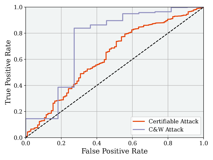
Figure 7: ROC Curve of Detection Results by Feature Squeezing on CIFAR10. The ROC score is $0.38$ and $0.26$ for the C&W attack and certifiable attack, respectively

Method	Attack $\sigma$	Defense $\sigma$	Ave. $\ell_{2}$-dis.	Rand. Query	Certified Acc.
Adaptive Denoiser	0.10	0.25	9.99	34.11	87.51%
Adaptive Denoiser	0.25	0.25	15.40	29.80	88.31%
Adaptive Denoiser	0.50	0.25	20.46	26.52	86.56%

Table 6: Performance of Certifiable Attack against the Adaptive Defenses on CIFAR10.

5.3 Performance against Adaptive Defenses

Furthermore, we consider a more challenging situation for the adversary for evaluating the certifiable attacks. We assume the model owner possesses different degrees of knowledge about the certifiable attack and will design some adaptive defenses against the certifiable attack. Certifiable attack injects noise to the inputs when querying the target model with the randomized inputs. We assume that the model owner knows the noise distribution that the adversary uses (strong defense in white-box setting). From the model owner’s perspective, we may deploy a CNN-based denoiser to eliminate these noise to resolve the certification for the attack. The denoiser is deployed as a pre-processing module and is pre-trained by the model owner.

Specifically, the model owner can train the denoiser to recover the noise-perturbed inputs back to the clean input, and also recover the adversarial features to normal features. Using a U-Net structure as the denoiser, we train the denoiser to remove the noise. Denoting the denoiser as $\mathcal{D}$, the loss function for the training is

$$\mathcal{L}=||\mathcal{D}(x+\epsilon)-x||_{2}+||f(\mathcal{D}(x+\epsilon))-f(x)||_{2}$$ (10)

Take Gaussian noise as an example (e.g., the model owner knows that Gaussian noise was used in the certifiable attack). In this experiment, we train the denoiser to eliminate Gaussian noise with $\sigma=0.25$ while evaluating the certifiable attack with Gaussian noise generated by different $\sigma$. The CASR is set to $p=90\%$. Table 6 illustrates that the denoiser defense can significantly degrade the performance of certifiable attack (by comparing Table 6 with Table 2). However, the certified accuracy is still near $90\%$.

5.4 Empirical Attack vs. Certifiable Attack

To our best knowledge, certifiable attack is a new paradigm of adversarial attacks. It is unfair to compare the empirical attacks with certifiable attacks since the empirical attacks cannot guarantee the attack success rate of any adversarial example. Moreover, the significance behind the accuracy metrics are different. The certified accuracy in certifiable attack means how much percentage of the test samples can be guaranteed to have the lower bound of the ASR, while the attack accuracy in empirical attack means how much percentage of the test samples on which can the empirical attack find successful adversarial examples.

However, in order to position the certifiable attack’s performance, we present the perturbation size and runtime of several empirical black-box attacks, as well as the certifiable attack. Specifically, we compare the certifiable attack with state-of-the-art black-box attacks including Square Attack [1], HopSkipJump Attack [9], and Geometric Decision-based Attack [39]. Table 7 presents that the overall average $\ell_{2}$-distance and the runtime of certifiable attack are relatively higher than the empirical attacks (our certifiable attack is faster than HopSkipJump). However, considering the benefits of provable guarantee to the attack success, these costs are worthwhile and tolerable for the adversaries.

Attack	$\sigma$	Ave. $\ell_{2}$-dis.	Runtime
Square Attack	–	7.76	0.16
HopSkipJump	–	0.15	16.94
GeoDA	–	5.40	2.42
Certifiable Attack	0.10	7.39	15.61
Certifiable Attack	0.25	12.95	14.12
Certifiable Attack	0.50	19.41	11.51

Table 7: Empirical Attack vs. Certifiable Attack on CIFAR10 (1,000 Monte Carlo samples; the runtime can be significantly reduced with less Monte Carlo samples)

6 Discussion

In this section, we discuss some issues related to the certifiable black-box attack.

Certifiable Attack Implementation. The certifiable attack does not have extra requirements on realization comparing to traditional black-box attacks. To implement the certifiable attack, it only needs to define a continuous noise distribution, and a CASR threshold. The certifiable attack can subvert any hard-label target models. The adversary will need to inject the noise into the adversarial examples, and query the target model. Then, PAE can be crafted by the randomized queries and our theory. Th attack was implemented on Pytorch [38].

Are Initialization and Shifting Necessary? The initialization is necessary since it meets the pre-condition of the guarantee. Without satisfaction on condition Eq. 4, the guarantee would be invalid. Shifting does not change the provable guarantee, but it is highly recommended since minimizing the perturbation size is also essential to adversarial attacks (for imperceptibility). Note that, the proposed initialization and shifting are only example methods. More optimal and efficient initialization and shifting methods can be designed to improve the performance of the certifiable attack.

Randomized Query vs. Traditional Queries. The randomized query returns a probability that the inputs are classified into false classes, while the traditional query returns a classification result for an input (provided by the adversary). The randomized query will execute a batch of traditional queries (depending on the number of Monte Carlo samples). Since these queries are based on the same adversarial inputs, they can be executed in parallel for query acceleration.

How Many Monte Carlo Samples are Enough to Craft a PAE with $p=90\%$? The number of Monte Carlo samples determines the lower bound of the $p_{adv}$, and further affects the shifting step length. Fewer number of Monte Carlo samples results in a smaller shifting step length, and will increase the shifting steps. Thus, the number of samples mainly affects the crafting time of PAE but merely affects the PAE itself. However, since the condition Eq. 4 is required, the number of samples should be large enough to compute a $\underline{p_{adv}}\geq p$. We present the relationship between Monte Carlo number and $\underline{p_{adv}}$ in Appendix E. It shows that $1,000$ Monte Carlo samples can produce $\underline{p_{adv}}\simeq 1.0$, and $250$ Monte Carlo samples are enough to produce $\underline{p_{adv}}\geq 90\%$. Therefore, we set the Monte Carlo number as $1,000$ in our experiments.

Mitigating the Certifiable Attacks. We have observed that many defense methods, e.g., adversarial training, randomized smoothing, and adaptive denoiser can mitigate the certifiable attacks, but the certifiable attacks can still achieve a relatively high certified accuracy. Are there any stronger adaptive methods that can effectively defend against certifiable attack completely? We may design a detection method to identify the noise from the inputs. Specifically, we can train a binary classifier to distinguish the noise-perturbed inputs and clean inputs. In the experiment, we leverage the ResNet110 to train a noise detector to detect the noise-perturbed adversarial examples. The experimental results show that the detction rate can be as high as $99\%$, which means the adaptive detection can be used as a strong defense against certifiable attack. However, as an adaptive defense, it is only specified to defend the certifiable attack. When deploying to the target model, it may consume much more computational resource since all the inputs have to go through the detection first. Moreover, this defense may not work once the noise scale or the noise area is reduced. Especially, the adversary may design a novel method to hide these noise into the image texture, which may circumvent the detection method.

Extension to Certifiable White-Box Attacks. The certifiable attack can be directly used as a white-box attack since it only requires the hard-label query access. To explore the potential of certifiable attack in the white-box setting, we may use a white-box initialization method. Specifically, the SSSP method can directly compute the gradients of the noise-perturbed examples rather than leveraging the feature extractor, which may significantly improve the certified accuracy of the certifiable attack.

Targeted Certifiable Attack. In this paper, we mainly focus on the untargeted certifiable attack. It is easy to craft a PAE in the untargeted setting since most of the classes are adversarial classes. However, if we perform certifiable attack by targeting specific class labels, it will be challenging to find a successful PAE since most of the noise-perturbed image should be limited to certain class(es). To tackle this problem, one may reduce the noise variance, which will increase the probability that most of the adversarial examples fall into the same class.

7 Conclusion

Certifiable attack lays a novel direction of adversarial attacks. We establish a novel theory to guarantee the attack success rate of adversarial examples by randomizing the queries with any continuous noise distribution in the black-box setting. Based on the theory, the adversary can craft the certifiable adversarial examples by two steps (the initialization and the shifting). The initialization aims to find a successful PAE (with provable attack success), and the shifting aims to reduce the perturbation size for better imperceptibility without affecting the provable attack success. In this paper, we give an example initialization method based on the smoothed self-supervised perturbation as well as an example shifting method based on the geometrically shifting. We comprehensively evaluate the performance of such new type of adversarial attacks in various circumstances against different defense methods. It is worthwhile to investigate more certifiable attack theories, more methods for crafting effective adversarial perturbations, and the corresponding countermeasures.

Appendix A Proof of Theorem 1

The proof of Theorem 1 is based on the Neyman-Pearson Lemma, so we first review the Neyman-Pearson Lemma.

Lemma 1.

(Neyman-Pearson Lemma) Let $X$ and $Y$ be random variables in $\mathbb{R}^{d}$ with densities $\mu_{X}$ and $\mu_{Y}$. Let $f:\mathbb{R}^{d}\rightarrow\{0,1\}$ be a random or deterministic function. Then:

(1) If $S=\{z\in\mathbb{R}^{d}:\frac{\mu_{Y}(z)}{\mu_{X}(z)}\leq{t}\}$ for some $t>0$ and $\mathbb{P}(f(X)=1)\geq\mathbb{P}(X\in S)$, then $\mathbb{P}(f(Y)=1)\geq\mathbb{P}(Y\in S)$;

(2) If $S=\{z\in\mathbb{R}^{d}:\frac{\mu_{Y}(z)}{\mu_{X}(z)}\geq{t}\}$ for some $t>0$ and $\mathbb{P}(f(X)=1)\leq\mathbb{P}(X\in S)$, then $\mathbb{P}(f(Y)=1)\leq\mathbb{P}(Y\in S)$.

Let $x_{o}\in\mathbb{R}^{d}$ be any clean input with label $y\in\mathcal{Y}$. Let $x$ be an adversarial example of $x_{o}$. Let noise $\epsilon$ been drawn from any continuous distribution $\mu$. Denote $X=x+\epsilon$, and $X_{adv}=x+\delta+\epsilon$. Thus, the random variable $X$ follows distribution $\mu(x)$ and the random variable $X_{adv}$ follows distribution $\mu(x-\delta)$. Let $f:\mathbb{R}^{d}\rightarrow\mathcal{Y}$ be any deterministic or random function. For each input $x_{o}$, we can consider two classes: $y$ or $\neq y$, so the problem can be considered as a binary classification problem.

Let the lower bound of randomized query on $x$ denoted as $\underline{p_{adv}}$, thus we have $Q(x)\geq\underline{p_{adv}}$. Define the half set:

$$A:=\{z:\frac{\mu(x-\delta)}{\mu(x)}\leq\tau\}$$ (11)

where the auxiliary parameter $\tau$ is picked to suffice:

$$\mathbb{P}(x\in A)=\mathbb{P}(\frac{\mu(x-\delta)}{\mu(x)}\leq\tau)=\underline{p_{adv}}$$ (12)

Suppose $p_{adv}$ and the CASR $p$ satisfy:

$$p_{adv}\geq p$$ (13)

Now we have

$$Q(x)=\mathbb{P}(f(x+\epsilon)\neq y)\geq p_{adv}=\mathbb{P}(x\in A)$$ (14)

Using Neyman-Pearson Lemma (considering $x$ as $X$ and $x+\delta$ as $Y$ in Neyman-Pearson Lemma, and $\neq y$ as class $1$), we have:

$$\mathbb{P}(f(x+\delta+\epsilon)\neq y)\geq\mathbb{P}((x+\delta)\in A)$$ (15)

which is equal to

$$\mathbb{P}(f(x+\delta+\epsilon)\neq y)\geq\mathbb{P}(\frac{\mu(x)}{\mu(x+\delta)}\leq\tau)$$ (16)

If $\mathbb{P}(\frac{\mu(x)}{\mu(x+\delta)}\leq\tau)\geq p$, we can guarantee that

$$\mathbb{P}(f(X_{adv})\neq y)=\mathbb{P}(f(x+\delta+\epsilon)\neq y)\geq p$$ (17)

so the PAE $X_{adv}$ can be guaranteed to have the CASR $p$.

Considering Eq. (12), we have

$$\tau=\Phi^{-1}_{-}(p_{adv})$$ (18)

where $\Phi^{-1}_{-}$ is the inverse Cumulative Density Function (CDF) of random variable $\frac{\mu(x-\delta)}{\mu(x)}$. Therefore, substitute $\tau$ in $\mathbb{P}(\frac{\mu(x)}{\mu(x+\delta)}\leq\tau)\geq p$, we have

$$\Phi_{+}(\Phi^{-1}_{-}(p_{adv}))\geq p$$ (19)

where $\Phi_{+}$ is the CDF of random variable $\frac{\mu(x)}{\mu(x+\delta)}$. The ratios can be simplified as

$$\frac{\mu(x-\delta)}{\mu(x)}=\frac{\mu(\epsilon-\delta)}{\mu(\epsilon)}$$ (20)

$$\frac{\mu(x)}{\mu(x+\delta)}=\frac{\mu(\epsilon)}{\mu(\epsilon+\delta)}$$ (21)

Now we complete the proof of Theorem 1.

Appendix B Certifiable Attack Theorem: Gaussian Noise

Corollary 1.2.

(Certifiable Adversarial Attack: Gaussian Noise) Let $f:\mathbb{R}^{d}\rightarrow\mathcal{Y}$ be any deterministic or random function, let $x_{o}$ be any clean input, $y$ be the label of $x_{o}$. Let $x$ be an adversarial example of $x_{o}$, $\delta$ be any perturbation, and $\epsilon$ be the noise drawn from Gaussian distribution $\mathcal{N}(0,\sigma)$. Denote $\underline{p_{adv}}\in[0,1]$ as the lower bound of the randomized query. If the randomized query on the adversarial input satisfies Eq. (4):

$$Q(x)=\mathbb{P}(f(x+\epsilon)\neq y)\geq\underline{p_{adv}}\geq p$$ (22)

Then, the probabilistic adversarial example $x_{adv}\equiv x+\delta+\epsilon$ is guaranteed to have certifiable attack success rate $p$ if the perturbation $\delta$ satisfies:

$$||\delta||_{2}\leq\sigma(\Phi^{-1}(p_{adv})-\Phi^{-1}(p))$$ (23)

where $\Phi^{-1}$ denotes the inverse of the standard Gaussian CDF.

Proof.

The Gaussian distribution is $\mu(x)\propto e^{-\frac{x^{2}}{2\sigma^{2}}}$, thus

$$\frac{\mu(x-\delta)}{\mu(x)}=e^{(2x\delta-\delta^{2})/(2\sigma^{2})}$$ (24)

Let $\tau:=exp((2\Phi_{\sigma}^{-1}(\underline{p_{adv}})\delta-\delta^{2})/(2\sigma^{2}))$, where $\Phi^{-1}_{\sigma}$ denotes the inverse Gaussian CDF with variance $\sigma$. Then we have:

$$\mathbb{P}(x\in A) =\mathbb{P}(\frac{\mu(x-\delta)}{\mu(x)}\leq\tau)$$ (25)

$$=\mathbb{P}(exp((2x\delta-\delta^{2})/(2\sigma^{2}))\leq$$ (26)

$$exp((2\Phi_{\sigma}^{-1}(\underline{p_{adv}})\delta-\delta^{2})/(2\sigma^{2})))$$ (27)

$$=\mathbb{P}(x\leq\Phi_{\sigma}^{-1}(\underline{p_{adv}}))$$ (28)

$$=\underline{p_{adv}}$$ (29)

Using Neyman-Pearson Lemma, we have:

$$\mathbb{P}(f(x+\delta+\epsilon)\neq y)\geq\mathbb{P}((x+\delta)\in A)$$ (31)

Since

$$\mathbb{P}((x+\delta)\in A) =\mathbb{P}(\frac{\mu(x)}{\mu(x+\delta)}\leq\tau)$$ (32)

$$=\mathbb{P}(exp((2x\delta+\delta^{2})/(2\sigma^{2}))\leq$$ (33)

$$exp((2\Phi_{\sigma}^{-1}(\underline{p_{adv}})\delta-\delta^{2})/(2\sigma^{2})))$$ (34)

$$=\mathbb{P}(2x\delta+\delta^{2}\leq(2\Phi_{\sigma}^{-1}(\underline{p_{adv}})\delta-\delta^{2}))$$ (35)

$$=\mathbb{P}(x\leq\Phi_{\sigma}^{-1}(\underline{p_{adv}})-||\delta||)$$ (36)

$$=\mathbb{P}(\frac{x}{\sigma}\leq\Phi^{-1}(\underline{p_{adv}})-\frac{||\delta||}{\sigma})$$ (37)

where $\Phi^{-1}$ denotes the inverse standard Gaussian CDF.

To guarantee that $\mathbb{P}(f(x+\delta+\epsilon)\neq y)\geq p$, we need:

$$\mathbb{P}((x+\delta)\in A) =\mathbb{P}(\frac{x}{\sigma}\leq\Phi^{-1}(\underline{p_{adv}})-\frac{||\delta||}{\sigma})$$ (38)

$$\geq p$$ (39)

which is equivalent to

$$||\delta||\leq\sigma(\Phi^{-1}(\underline{p_{adv}})-\Phi^{-1}(p))$$ (41)

This completes the proof of Corollary 1.2.

∎

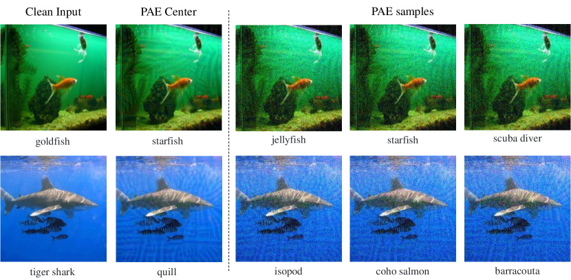
Figure 8: PAE Examples on ImageNet with $\sigma=0.1$ and $p=0.9$. Images have been misclassified with the adversarial example crafted at the PAE Center (provable) and all the PAE samples have 90%+ confidence to be misclassified

Appendix C Proof of Proposition 1

If the Condition Eq. (4) is satisfied, we have

$$\underline{p_{adv}}\geq p$$ (42)

For any direction $w$, our goal is to find the $\delta$ in this direction with maximum $||\delta||_{2}$. When $||\delta||_{2}=0$, we have

$$\Phi_{+}=\Phi_{-}$$ (43)

Thus, we have

$$\Phi_{+}(\Phi^{-1}_{-}(p_{adv}))=p_{adv}\geq p$$ (44)

Then, we prove that when $||\delta||_{2}$ increase, we will get $\Phi_{+}(\Phi^{-1}_{-}(p_{adv}))$ decrease.

Since $\Phi_{-}$ is the CDF of the random variable $\frac{\mu(\epsilon-\delta)}{\mu(\epsilon)}$, and $\mu(x)$ decreases when $|x|$ increases, when $||\delta||_{2}\rightarrow\infty$, we have $\frac{\mu(\epsilon-\delta)}{\mu(\epsilon)}\rightarrow 0$, and $\Phi_{-}^{-1}(p_{adv})\rightarrow 0$.

Since $\Phi_{+}$ is the CDF of the random variable $\frac{\mu(\epsilon)}{\mu(\epsilon+\epsilon)}$, when $||\delta||_{2}\rightarrow\infty$, $\frac{\mu(\epsilon)}{\mu(\epsilon+\epsilon)}\rightarrow\infty$, so $\Phi_{+}\rightarrow 0$.

Therefore, when $||\delta||_{2}\rightarrow\infty$, we have

$$\Phi_{+}(\Phi^{-1}_{-}(p_{adv}))\rightarrow 0<p$$ (45)

When $||\delta||_{2}\rightarrow 0$, we have

$$\Phi_{+}(\Phi^{-1}_{-}(p_{adv}))=p_{adv}\geq p$$ (46)

Since $\Phi_{-}$ and $\Phi_{+}$ is continuous function, between $0$ and $\infty$, there must be some $\delta$ such that $\Phi_{+}(\Phi^{-1}_{-}(p_{adv}))=p$.

Now we prove that the binary search algorithm can always find the $\delta$ solution, then we show how to bound the adversarial attack certification. We use Monte Carlo method to estimate the $p_{adv}$ as well as the CDFs $\Phi_{-}$ and $\Phi_{+}$. To bound the empirical CDFs, we leverage Dvoretzky-Kiefer-Wolfowitz inequality [16].

Lemma 2.

(Dvoretzky–Kiefer–Wolfowitz inequality (restate)) Let $X_{1},X_{2},...,X_{n}$ be real-valued independent and identically distributed random variables with cumulative distribution function $F(\cdot)$, where $n\in\mathbb{N}$.Let $F_{n}$ denotes the associated empirical distribution function defined by

$$F_{n}(x)=\frac{1}{n}\sum_{i=1}^{n}\mathbf{1}_{\{X_{i}<=x\}},x\in\mathbb{R}$$ (47)

The Dvoretzky–Kiefer–Wolfowitz inequality bounds the probability that the random function $F_{n}$ differs from $F$ by more than a given constant $\Delta\in\mathbb{R}^{+}$ :

$$\mathbb{P}(\sup_{x\in\mathbb{R}}|F_{n}(x)-F(x)|>\Delta)\leq 2e^{-2n\Delta^{2}}$$ (48)

Let the Monte Carlo sampling number $N_{m}$. Each shifting is an independent certification, and there are a lower-bound estimation and two CDF estimation in each certification. Suppose the confidence of lower-bound estimation is $(1-\alpha_{o})$, then the certification confidence should be at least $(1-\alpha_{o})(1-2e^{-2N_{m}\Delta^{2}})^{2}$.

Appendix D Visualization

We visualize the adversarial examples sampled from the PAEs. The visualization is presented in Figure 8. The noise variance is set to $0.1$, so the adversarial examples are classified into more close classes. From left to right, we present the clean input, the center of the PAE, and several adversarial examples drawn from the PAE. In the first row, we show that a “goldfish” example is perturbed to “jellyfish”, “’starfish”, and “scuba diver” in different samples drawn from the PAE. In the second row, we show that a “tiger shark” example is perturbed to “isopod”, “coho salmon”, and “barracouta” in different samples drawn from the PAE.

Appendix E Number of Monte Carlo Samples vs. $\underline{p_{adv}}$

We present the relationship between the Monte Carlo sampling number and the lower bound of the $p_{adv}$ in Figure 9. The lower bound of the $p_{adv}$ is computed by the Binomial test, which depends on the Monte Carlo sampling number and the ratio of the correct samples and total samples. We set confidence parameter $\alpha=0.001$ and assume that all the samples are classified as adversarial classes, i.e., the ratio of correct samples and total samples is set to $1.0$. We observe that when Monte Carlo sample number is around $100$, it is enough to produce a $\underline{p_{adv}}\geq 0.9$. The $\underline{p_{adv}}$ is around $1.0$ when the Monte Carlo number is reaching $1,000$. When the Monte Carlo number is larger than $1,000$, the $\underline{p_{adv}}$ will gradually reach $1.0$. By balancing the $\underline{p_{adv}}$ and the running time, we set the Monte Carlo number as $1,000$ in our experiments.

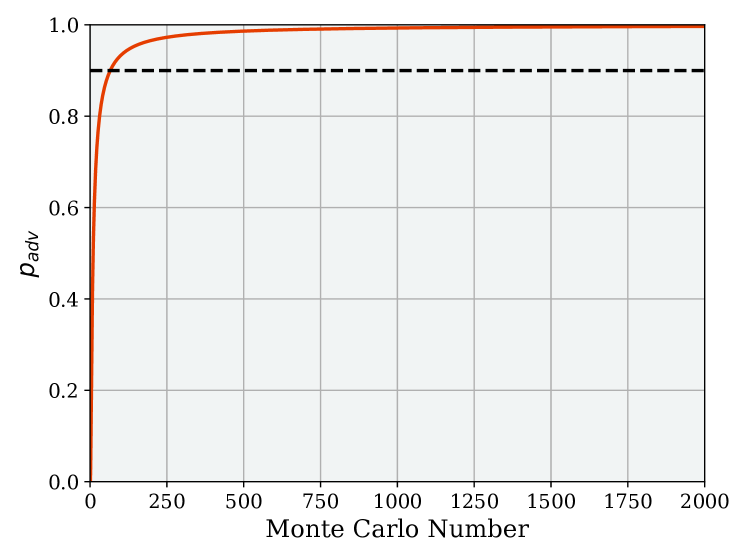
Figure 9: $\underline{p_{adv}}$ vs. Number of Monte Carlo Samples.

References

- [1] Maksym Andriushchenko, Francesco Croce, Nicolas Flammarion and Matthias Hein “Square Attack: A Query-Efficient Black-Box Adversarial Attack via Random Search” In ECCV, Lecture Notes in Computer Science, 2020 DOI: 10.1007/978-3-030-58592-1“˙29
- [2] Cem Anil, James Lucas and Roger B. Grosse “Sorting Out Lipschitz Function Approximation” In ICML, Proceedings of Machine Learning Research, 2019 URL: http://proceedings.mlr.press/v97/anil19a.html
- [3] Arjun Nitin Bhagoji, Warren He, Bo Li and Dawn Song “Practical Black-Box Attacks on Deep Neural Networks Using Efficient Query Mechanisms” In ECCV 11216 Springer, 2018, pp. 158–174 DOI: 10.1007/978-3-030-01258-8“˙10
- [4] Siddhant Bhambri, Sumanyu Muku, Avinash Tulasi and Arun Balaji Buduru “A survey of black-box adversarial attacks on computer vision models” In arXiv preprint arXiv:1912.01667, 2019
- [5] Wieland Brendel, Jonas Rauber and Matthias Bethge “Decision-Based Adversarial Attacks: Reliable Attacks Against Black-Box Machine Learning Models” In ICLR OpenReview.net, 2018 URL: https://openreview.net/forum?id=SyZI0GWCZ
- [6] Thomas Brunner, Frederik Diehl, Michael Truong-Le and Alois C. Knoll “Guessing Smart: Biased Sampling for Efficient Black-Box Adversarial Attacks” In ICCV, 2019, pp. 4957–4965 DOI: 10.1109/ICCV.2019.00506
- [7] Jacob Buckman, Aurko Roy, Colin Raffel and Ian J. Goodfellow “Thermometer Encoding: One Hot Way To Resist Adversarial Examples” In ICLR OpenReview.net, 2018 URL: https://openreview.net/forum?id=S18Su--CW
- [8] Nicholas Carlini and David A. Wagner “Towards Evaluating the Robustness of Neural Networks” In 2017 IEEE Symposium on Security and Privacy IEEE Computer Society, 2017 DOI: 10.1109/SP.2017.49
- [9] Jianbo Chen, Michael I. Jordan and Martin J. Wainwright “HopSkipJumpAttack: A Query-Efficient Decision-Based Attack” In IEEE Symposium on Security and Privacy, 2020, pp. 1277–1294 DOI: 10.1109/SP40000.2020.00045
- [10] Pin-Yu Chen et al. “ZOO: Zeroth Order Optimization Based Black-box Attacks to Deep Neural Networks without Training Substitute Models” In AISec@CCS ACM, 2017, pp. 15–26 DOI: 10.1145/3128572.3140448
- [11] Minhao Cheng et al. “Query-Efficient Hard-label Black-box Attack: An Optimization-based Approach” In ICLR, 2019 URL: https://openreview.net/forum?id=rJlk6iRqKX
- [12] Jeremy M. Cohen, Elan Rosenfeld and J. Kolter “Certified Adversarial Robustness via Randomized Smoothing” In ICML, 2019 URL: http://proceedings.mlr.press/v97/cohen19c.html
- [13] Guneet S. Dhillon et al. “Stochastic Activation Pruning for Robust Adversarial Defense” In ICLR, 2018 URL: https://openreview.net/forum?id=H1uR4GZRZ
- [14] Yinpeng Dong, Tianyu Pang, Hang Su and Jun Zhu “Evading Defenses to Transferable Adversarial Examples by Translation-Invariant Attacks” In IEEE Conference on Computer Vision and Pattern Recognition, CVPR 2019 Computer Vision Foundation / IEEE, 2019 DOI: 10.1109/CVPR.2019.00444
- [15] Yali Du et al. “Towards Query Efficient Black-box Attacks: An Input-free Perspective” In Proceedings of the 11th ACM Workshop on Artificial Intelligence and Security, CCS 2018, 2018 DOI: 10.1145/3270101.3270106
- [16] Aryeh Dvoretzky, Jack Kiefer and Jacob Wolfowitz “Asymptotic minimax character of the sample distribution function and of the classical multinomial estimator” In The Annals of Mathematical Statistics JSTOR, 1956, pp. 642–669
- [17] Matteo Fischetti and Jason Jo “Deep neural networks and mixed integer linear optimization” In Constraints An Int. J. 23.3, 2018, pp. 296–309 DOI: 10.1007/s10601-018-9285-6
- [18] Ian J. Goodfellow, Jonathon Shlens and Christian Szegedy “Explaining and Harnessing Adversarial Examples” In 3rd International Conference on Learning Representations, ICLR 2015, 2015
- [19] Chuan Guo, Mayank Rana, Moustapha Cissé and Laurens Maaten “Countering Adversarial Images using Input Transformations” In 6th International Conference on Learning Representations, ICLR 2018 OpenReview.net, 2018 URL: https://openreview.net/forum?id=SyJ7ClWCb
- [20] Chuan Guo et al. “Simple Black-box Adversarial Attacks” In Proceedings of the 36th International Conference on Machine Learning, ICML 2019, Proceedings of Machine Learning Research, 2019 URL: http://proceedings.mlr.press/v97/guo19a.html
- [21] Hanbin Hong, Binghui Wang and Yuan Hong “UniCR: Universally Approximated Certified Robustness via Randomized Smoothing” In arXiv preprint arXiv:2207.02152, 2022
- [22] Andrew Ilyas, Logan Engstrom, Anish Athalye and Jessy Lin “Black-box Adversarial Attacks with Limited Queries and Information” In Proceedings of the 35th International Conference on Machine Learning, ICML 2018, Proceedings of Machine Learning Research PMLR, 2018 URL: http://proceedings.mlr.press/v80/ilyas18a.html
- [23] Andrew Ilyas, Logan Engstrom, Anish Athalye and Jessy Lin “Query-Efficient Black-box Adversarial Examples” In CoRR abs/1712.07113, 2017 arXiv: http://arxiv.org/abs/1712.07113
- [24] Shubham Jain, Ana-Maria Crețu and Yves-Alexandre Montjoye “Adversarial Detection Avoidance Attacks: Evaluating the robustness of perceptual hashing-based client-side scanning” In 31st USENIX Security Symposium (USENIX Security 22), 2022, pp. 2317–2334
- [25] Guy Katz et al. “Reluplex: An Efficient SMT Solver for Verifying Deep Neural Networks” In Computer Aided Verification - 29th International Conference, CAV 2017 DOI: 10.1007/978-3-319-63387-9“˙5
- [26] Kate Keahey et al. “Lessons Learned from the Chameleon Testbed” In Proceedings of the 2020 USENIX Annual Technical Conference (USENIX ATC ’20) USENIX Association, 2020
- [27] Alex Krizhevsky and Geoffrey Hinton “Learning multiple layers of features from tiny images” Citeseer, 2009
- [28] Alexey Kurakin, Ian J. Goodfellow and Samy Bengio “Adversarial Machine Learning at Scale” In 5th International Conference on Learning Representations, ICLR 2017 OpenReview.net, 2017
- [29] Yandong Li et al. “NATTACK: Learning the Distributions of Adversarial Examples for an Improved Black-Box Attack on Deep Neural Networks” In Proceedings of the 36th International Conference on Machine Learning, ICML 2019, Proceedings of Machine Learning Research URL: http://proceedings.mlr.press/v97/li19g.html
- [30] Fangzhou Liao et al. “Defense Against Adversarial Attacks Using High-Level Representation Guided Denoiser” In 2018 IEEE Conference on Computer Vision and Pattern Recognition, CVPR 2018 Computer Vision Foundation / IEEE Computer Society DOI: 10.1109/CVPR.2018.00191
- [31] Jiajun Lu, Theerasit Issaranon and David A. Forsyth “SafetyNet: Detecting and Rejecting Adversarial Examples Robustly” In IEEE International Conference on Computer Vision, ICCV 2017 DOI: 10.1109/ICCV.2017.56
- [32] Aleksander Madry et al. “Towards Deep Learning Models Resistant to Adversarial Attacks” In 6th International Conference on Learning Representations, ICLR 2018 OpenReview.net, 2018 URL: https://openreview.net/forum?id=rJzIBfZAb
- [33] Dongyu Meng and Hao Chen “MagNet: A Two-Pronged Defense against Adversarial Examples” In Proceedings of the 2017 ACM SIGSAC Conference on Computer and Communications Security, CCS 2017 DOI: 10.1145/3133956.3134057
- [34] Seyed-Mohsen Moosavi-Dezfooli, Alhussein Fawzi, Omar Fawzi and Pascal Frossard “Universal adversarial perturbations” In CoRR abs/1610.08401, 2016 arXiv: http://arxiv.org/abs/1610.08401
- [35] Muzammal Naseer et al. “A Self-supervised Approach for Adversarial Robustness” In 2020 IEEE/CVF Conference on Computer Vision and Pattern Recognition, CVPR 2020 Computer Vision Foundation / IEEE, 2020, pp. 259–268 DOI: 10.1109/CVPR42600.2020.00034
- [36] Nicolas Papernot et al. “Distillation as a Defense to Adversarial Perturbations Against Deep Neural Networks” In IEEE Symposium on Security and Privacy, SP 2016 IEEE Computer Society, 2016, pp. 582–597 DOI: 10.1109/SP.2016.41
- [37] Nicolas Papernot et al. “Practical Black-Box Attacks against Machine Learning” In Proceedings of the 2017 ACM on Asia Conference on Computer and Communications Security, AsiaCCS 2017 ACM DOI: 10.1145/3052973.3053009
- [38] Adam Paszke et al. “PyTorch: An Imperative Style, High-Performance Deep Learning Library” In Advances in Neural Information Processing Systems 32 Curran Associates, Inc.
- [39] Ali Rahmati, Seyed-Mohsen Moosavi-Dezfooli, Pascal Frossard and Huaiyu Dai “Geoda: a geometric framework for black-box adversarial attacks” In Proceedings of the IEEE/CVF conference on computer vision and pattern recognition, 2020, pp. 8446–8455
- [40] Kevin Roth, Yannic Kilcher and Thomas Hofmann “The Odds are Odd: A Statistical Test for Detecting Adversarial Examples” In Proceedings of the 36th International Conference on Machine Learning, ICML 2019, Proceedings of Machine Learning Research URL: http://proceedings.mlr.press/v97/roth19a.html
- [41] Olga Russakovsky et al. “ImageNet Large Scale Visual Recognition Challenge” In International Journal of Computer Vision (IJCV) 115.3, 2015, pp. 211–252 DOI: 10.1007/s11263-015-0816-y
- [42] Pouya Samangouei, Maya Kabkab and Rama Chellappa “Defense-GAN: Protecting Classifiers Against Adversarial Attacks Using Generative Models” In 6th International Conference on Learning Representations, ICLR 2018 OpenReview.net, 2018 URL: https://openreview.net/forum?id=BkJ3ibb0-
- [43] Ali Shafahi et al. “Adversarial training for free!” In Advances in Neural Information Processing Systems 32: Annual Conference on Neural Information Processing Systems 2019, NeurIPS 2019, 2019, pp. 3353–3364 URL: https://proceedings.neurips.cc/paper/2019/hash/7503cfacd12053d309b6bed5c89de212-Abstract.html
- [44] Yucheng Shi, Siyu Wang and Yahong Han “Curls & Whey: Boosting Black-Box Adversarial Attacks” In IEEE Conference on Computer Vision and Pattern Recognition, CVPR 2019 Computer Vision Foundation / IEEE, 2019, pp. 6519–6527 DOI: 10.1109/CVPR.2019.00668
- [45] Yang Song et al. “PixelDefend: Leveraging Generative Models to Understand and Defend against Adversarial Examples” In 6th International Conference on Learning Representations, ICLR 2018 OpenReview.net, 2018 URL: https://openreview.net/forum?id=rJUYGxbCW
- [46] Jiaye Teng, Guang-He Lee and Yang Yuan “ Adversarial Robustness Certificates: a Randomized Smoothing Approach”, 2019
- [47] Florian Tramèr “Detecting Adversarial Examples Is (Nearly) As Hard As Classifying Them” In International Conference on Machine Learning, ICML 2022, Proceedings of Machine Learning Research URL: https://proceedings.mlr.press/v162/tramer22a.html
- [48] Florian Tramèr and Dan Boneh “Adversarial Training and Robustness for Multiple Perturbations” In Advances in Neural Information Processing Systems, NeurIPS 2019 URL: https://proceedings.neurips.cc/paper/2019/hash/5d4ae76f053f8f2516ad12961ef7fe97-Abstract.html
- [49] Florian Tramèr et al. “Ensemble Adversarial Training: Attacks and Defenses” In 6th International Conference on Learning Representations, ICLR 2018 URL: https://openreview.net/forum?id=rkZvSe-RZ
- [50] Eric Wong and J. Kolter “Provable Defenses against Adversarial Examples via the Convex Outer Adversarial Polytope” In Proceedings of the 35th International Conference on Machine Learning, ICML 2018 URL: http://proceedings.mlr.press/v80/wong18a.html
- [51] Eric Wong, Frank R. Schmidt and J. Kolter “Wasserstein Adversarial Examples via Projected Sinkhorn Iterations” In Proceedings of the 36th International Conference on Machine Learning, ICML 2019, Proceedings of Machine Learning Research PMLR URL: http://proceedings.mlr.press/v97/wong19a.html
- [52] Cihang Xie et al. “Mitigating Adversarial Effects Through Randomization” In 6th International Conference on Learning Representations, ICLR 2018 OpenReview.net, 2018 URL: https://openreview.net/forum?id=Sk9yuql0Z
- [53] Shangyu Xie, Han Wang, Yu Kong and Yuan Hong “Universal 3-Dimensional Perturbations for Black-Box Attacks on Video Recognition Systems” In In Proceedings of the 43rd IEEE Symposium on Security and Privacy, 2022
- [54] Weilin Xu, David Evans and Yanjun Qi “Feature squeezing: Detecting adversarial examples in deep neural networks” In arXiv preprint arXiv:1704.01155, 2017
- [55] Greg Yang et al. “Randomized Smoothing of All Shapes and Sizes” In ICML, Proceedings of Machine Learning Research, 2020 URL: http://proceedings.mlr.press/v119/yang20c.html