Ensemble Modeling for Time Series Forecasting: an Adaptive Robust Optimization Approach

Abstract

Accurate time series forecasting is critical for a wide range of problems with temporal data. Ensemble modeling is a well-established technique for leveraging multiple predictive models to increase accuracy and robustness, as the performance of a single predictor can be highly variable due to shifts in the underlying data distribution. This paper proposes a new methodology for building robust ensembles of time series forecasting models. Our approach utilizes Adaptive Robust Optimization (ARO) to construct a linear regression ensemble in which the models’ weights can adapt over time. We demonstrate the effectiveness of our method through a series of synthetic experiments and real-world applications, including air pollution management, energy consumption forecasting, and tropical cyclone intensity forecasting. Our results show that our adaptive ensembles outperform the best ensemble member in hindsight by 16-26% in root mean square error and 14-28% in conditional value at risk and improve over competitive ensemble techniques.

Keywords: time series forecasting, ensemble modeling, regression, robust and adaptive optimization, sustainability

1 Introduction

Time series data capture sequential measurements and observations indexed by timestamps. The unique characteristics of time series data, in which observations have a chronological order, often make their analysis challenging. In particular, predicting future target values through time series forecasting is a critical research topic in many real-world applications with a temporal component, such as healthcare operations, finance, energy, climate, and business. Organizations and professionals often use forecasting to inform their decision-making, anticipate uncertain scenarios, and take proactive measures.

Many popular forecasting methods exist, including auto-regressive processes (Hamilton, 2020; Hyndman and Athanasopoulos, 2021), exponential smoothing approaches (Gardner Jr., 1985), and neural networks (Salinas et al., 2020; Lara-Benítez et al., 2021). Another common approach consists in converting a time series into a non-temporal format by concatenating several time steps of data to use classic machine learning models, such as gradient-boosted trees (Makridakis et al., 2022). However, no forecasting method consistently outperforms others as modeling assumptions may have to change over time to account for the often complex mechanisms behind the time series generation (Chatfield, 2000). As a result, the accuracy of each forecasting method can vary significantly across time depending on model drift (Gama et al., 2014).

Ensemble modeling is a well-established technique to leverage the strengths and limitations of multiple models and benefit from their diversity (Dietterich, 2000; Brown and Kuncheva, 2010; Oliveira and Torgo, 2015). The principle is to combine the predictions of the forecasting models available to obtain a more accurate, stable, and robust predictor. This approach has gained widespread attention with a variety of methods, including the concepts of stacking (Wolpert, 1992), bagging (Breiman, 1996b), or boosting (Schapire, 1990; Breiman, 1996a; Chen and Guestrin, 2016).

When applied to time series forecasting, ensemble modeling can become a complex task, as the temporal aspect of the data adds difficulty in determining which model is most suitable at any given point in time (Oliveira and Torgo, 2015; Cerqueira et al., 2020). A common approach is to weigh the ensemble members based on their performance in recent or historical observations, assuming the data distribution will stay similar and models behave consistently. Other approaches include meta-learning (Prudêncio and Ludermir, 2004; Gastinger et al., 2021) or regret minimization, for example, under the multi-armed bandit setting (Cesa-Bianchi and Lugosi, 2006).

However, these methods do not necessarily enforce the robustness of the ensembles, which can lead to critical prediction errors. In this study, we propose to explore ensemble modeling for time series forecasting from a different perspective, using robust optimization. We present a novel optimization scheme that dynamically selects the weights of an ensemble of forecasts at each time step, taking into account the uncertainty and errors of the underlying forecasts. Our approach is based on multi-stage robust optimization, where the weights are optimized variables determined at each time step in response to newly revealed information about the uncertain parameters.

Traditional optimization assumes that all optimization variables are “here and now” decisions, i.e., we have to determine the values for these optimization variables now and cannot wait for more information on the uncertain parameters. However, in multi-stage (dynamic) decision problems, we can introduce “wait and see” variables that can be determined after the uncertain parameter values have been revealed (Bertsimas and den Hertog, 2022). Although this modeling process is challenging to implement in practice, it offers powerful guarantees for robust dynamic decision-making under uncertainty.

The Adaptive Robust Optimization (ARO) framework is a methodology to address multi-stage problems by adjusting wait-and-see variables as a function of uncertain parameters. By utilizing ARO, we aim to demonstrate the viability of creating a new branch of ensemble methods for temporal tasks, leveraging the strengths of adaptive robust methods. The results of our work showcase the exciting potential of ARO for applications in the field of machine learning. Our contributions include:

1. A novel ensemble method that leverages the ARO framework to dynamically adjust the weights of underlying models in real time, resulting in a robust and accurate forecasting tool. Our approach, based on linear regression ensembles, is detailed in Section 3.

2. An analysis of the robustness guarantees of our method, accompanied by equivalent formulations for easy and tractable implementation, as outlined in Section 3.4.

3. A comprehensive study of the impact of various hyperparameters on our adaptive ensemble method, as demonstrated through synthetic experiments in Section 4.

4. Empirical validation of our proposed ensemble method, showcasing its superiority over existing ensemble methods across multiple real-world forecasting applications, including wind speed forecasting for air pollution management, energy consumption forecasting, and tropical cyclone intensity forecasting (see Figure 1). Our method outperforms the best ensemble member in hindsight by 16-26% in terms of root mean square error and 14-28% in conditional value at risk with a 15% threshold, as demonstrated in Section 5.

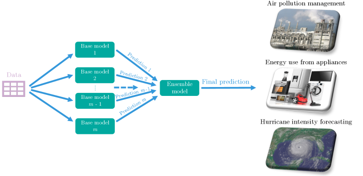
Figure 1: Schematic of the principle of ensemble modeling. Several base learners make predictions from the original data and are combined into an ensemble. We represent the three real-world data applications included in this paper.

2 Background

This section briefly reviews standard ensemble methods for time series forecasting before introducing the field of robust and adaptive optimization.

2.1 Ensemble Methods for Time Series Forecasting

Linear Ensembles

After the seminal work of Bates and Granger (1969), several combination methodologies were added to the forecaster toolbox (Clemen, 1989; Zou and Yang, 2004). In particular, weighted linear combinations of different ensemble members became popular due to the straightforward implementation for real-world deployment. Some typical linear combination techniques include the simple average, trimmed average, winsorized average, or median of the ensemble members’ forecasts. Other methodologies can weigh the models based on their past errors, respective performance, or variance. For instance, one can train a regularized linear regression such as Ridge (Hoerl and Kennard, 1970) or LASSO (Tibshirani, 1996) to ensemble the different forecasts. See Adhikari and Agrawal (2012) for a thorough review of linear ensemble methods.

Model Drift

In general, the weighted ensembles are often designed and trained using some historical observations and then deployed as fixed. While this is convenient for deployment purposes, this static setting may represent limitations when there is model drift, i.e., potential degradation of a model’s predictive power due to changes in the data. In this case, the ensemble members’ performance can vary across time or different events due to “data drift” or “concept drift”. Data drift refers to the model drift scenario when the properties of the independent variables’ distribution change, for example, due to seasonality, a shift in consumer behaviors or company strategies, or unexpected events. On the other hand, concept drift corresponds to the scenario when the properties of the dependent variable change, which can happen because of changes in the definition of the target value, the annotation methodology, or the target sensor.

Dynamic Ensemblers

Another common approach to ensemble forecasting consists in dynamically changing the weights of the different models in response to model drift (Kuncheva, 2004; Gama et al., 2014). In particular, the multi-armed bandit settings have been widely investigated (Cesa-Bianchi and Lugosi, 2006). Numerous methods with different assumptions and contexts exist to track the losses of the ensemble members and find regret guarantees of the ensemble with respect to the best model of the ensemble: for instance, the Exp3, Upper-Confidence Bound, Online Passive-Aggressive (Crammer et al., 2006) algorithms (see Lattimore and Szepesvári (2020) for a complete review).

These algorithms dynamically combine the forecasting models at each time step by considering the problem of minimizing the multi-armed bandit regret against the best ensemble member.

2.2 Robust Optimization

Robust Optimization (RO) seeks to immunize models and problem formulations from adversarial perturbations in the data by introducing, in general, an uncertainty set that captures the deterministic assumptions about these perturbations. The objective is to find solutions that are still good or feasible under a general level of uncertainty and are called robust against errors of the specific magnitude and type chosen by the practitioner.

RO has gained substantial traction in recent years due to the guarantees provided to properly designed formulations and the progress of techniques and software to solve min-max adversarial optimization formulations (Bertsimas and den Hertog, 2022).

Formalism

We introduce some quick formalism to explicit the RO framework. We define a decision vector x in a compact set of possible decisions $\mathcal{X}$ and an ensemble of parameters $\textbf{z}\in\mathbb{R}^{n_{z}},{n_{z}}\geq 0$ representing the information available in the problem. Our optimization problem aims to minimize some objective function $f(\textbf{z},\textbf{x})$. We may also specify a set of constraints $f_{i}(\textbf{z},\textbf{x})\leq 0,i\in[p]$, where we assume $f_{i}(\cdot,\textbf{x})$ is convex in x. Overall, we are interested in solving problems in this initial form:

$$\min_{\textbf{x}\in\mathcal{X}}\; f(\textbf{z},\textbf{x})$$

s.t. $$f_{i}(\textbf{z},\textbf{x})\leq 0,\quad\forall i\in[p].$$

When z is readily available, we can solve this problem with classical optimization methods. However, z is uncertain and rarely explicitly known in real-world applications. The robust optimization approach consists in representing the set of possible values of z with an uncertainty set $\mathcal{Z}$ and solving for the decision x such that the constraints $f_{i}$ are always satisfied. We now optimize $f$ for the worst case, and the problem becomes:

$$\min_{\textbf{x}\in\mathcal{X}}\max_{\textbf{z}\in\mathcal{Z}}\; f(\textbf{z},\textbf{x})$$

s.t. $$f_{i}(\textbf{z},\textbf{x})\leq 0,\quad\forall i\in[p],\quad\forall\textbf{z}\in\mathcal{Z}.$$

The adversarial nature of such a problem can make it very difficult to solve to optimality. A key aspect of RO is to derive an equivalent reformulation of a robust problem with a computationally tractable form.

2.3 Adaptive Robust Optimization

Adaptive robust optimization (ARO) expands the RO framework by separating the decision x into multiple stages. The principle of a multi-stage problem is to contain adaptive “wait-and-see” decisions in addition to urgent “here-and-now” decisions. With ARO, once the “here-and-now” decisions are made, we consider that some of the uncertain parameters will become known before determining the “wait-and-see” decisions.

This multi-stage setting encompasses many real-world scenarios, such as lot-sizing on a network, product inventory systems, unit commitment, and factory location problems, e.g., (Bertsimas et al., 2013; Bertsimas and Georghiou, 2015).

Formally, we denote the adaptive decisions as $\textbf{y}(\textbf{z})$ since they are selected only after some of the uncertain parameters z may be revealed. An ARO problem typically writes as:

$$\min_{\textbf{x}\in\mathcal{X},\textbf{y}(\textbf{z})}\max_{\textbf{z}\in\mathcal{Z}}\; f(\textbf{z},\textbf{x},\textbf{y}(\textbf{z}))$$

s.t. $$f_{i}(\textbf{z},\textbf{x},\textbf{y}(\textbf{z}))\leq 0,\quad\forall i\in[p].$$

Note that expressing y as a function of z allows the practitioner to choose the function $\textbf{y}(\textbf{z})$ arbitrarily before learning z, which is then called a decision rule.

In general, problems that contain such constraints with decision rules are NP-hard (Ben-Tal et al., 2004). Therefore, to make them tractable, we may restrict $\textbf{y}(\textbf{z})$ to a given class of functions even though it could be sup-optimal. One such class is the affine decision rule, which conveniently expresses $\textbf{y}(\textbf{z})$ with an affine relationship with z: $\textbf{y}(\textbf{z})=\textbf{x}_{0}+\mathbf{V}\cdot\textbf{z}$, where the coefficients $\textbf{x}_{0}$ and $\mathbf{V}$ are to be determined and become “here-and-now” decision variables. Using decision rules is one of ARO’s core ideas that will serve this paper’s methodology.

3 The Problem: a Robust Linear Regression for Time Series Forecasting

We aim to formulate an adaptive version of a robust linear regression problem, such as Ridge or LASSO, in ensemble modeling for time series forecasting. We show how to develop an adaptive robust formulation that leverages the temporal aspect of the data and guarantees specific protection against model drift.

3.1 Linear Regression for a Time Series Ensemble

Define a sample $\mathbf{X}_{t}=[x_{t}^{1},\dots,x_{t}^{m}]\in\mathbb{R}^{m}$ as the forecasts made by $m$ individual models at time $t$ for the same fixed lead time period. We call these $m$ models ensemble members. We consider we are given a historical time series of ensemble members’ predictions $(\mathbf{X},\mathbf{y})\in(\mathbb{R}^{T\times m}\times\mathbb{R}^{T})$ with $T$ regularly spaced samples $\mathbf{X}_{t}\in\mathbb{R}^{m}$ with the corresponding ground-truth values $y_{t}\in\mathbb{R}$.

Since we are interested in a dynamic linear combination of the forecasts, we associate all ensemble member predictions to time-varying coefficients $\boldsymbol{\beta}_{t}=[\beta_{t}^{1},\dots,\beta_{t}^{m}]\in\mathbb{R}^{m}$. For compactness, we also define the vector of coefficients:

$$\boldsymbol{\beta}:=[\boldsymbol{\beta}_{1}|\dots|\boldsymbol{\beta}_{T}]=[\beta_{1}^{1},\dots,\beta_{1}^{m},\dots,\beta_{T}^{1},\dots,\beta_{T}^{m}]\in\Omega\subset\mathbb{R}^{T\cdot m},$$

where $\Omega$ is a user-designed set of constraints on the coefficients, and $|$ is the concatenation operation.

To build an adaptive weighted ensemble to approximate the ground truth values, we are interested in minimizing problems similar to the following ordinary least squares problem:

$$\begin{array}[]{ll}\displaystyle\min_{\boldsymbol{\beta}\in\Omega}&\displaystyle\sqrt{\sum_{t=1}^{T}\left(y_{t}-\mathbf{X}^{\top}_{t}\boldsymbol{\beta}_{t}\right)^{2}},\\ \end{array}$$ (1)

or the least absolute deviation problem written as follows:

$$\begin{array}[]{ll}\displaystyle\min_{\boldsymbol{\beta}\in\Omega}&\displaystyle\sum_{t=1}^{T}\left|y_{t}-\mathbf{X}^{\top}_{t}\boldsymbol{\beta}_{t}\right|.\\ \end{array}$$ (2)

Before proceeding, we make several remarks about the settings in this paper:

• We allow $\boldsymbol{\beta}_{t}$ to vary over time, as we want more flexibility to capture the fluctuations in the forecast skills. We will define potential constraints on $\boldsymbol{\beta}\in\Omega$ later.

• We consider the complete observation of the forecasts and targets for a history of $T$ time steps. We assume access to historical data that can serve as training and validation sets.

• We assume that each time step is regularly spaced. However, the lead time for prediction is not necessarily one time step. For example, we can consider 6 hours between each time step, and make forecasts for 24 hours later, i.e., for a given time step $t$, $y_{t}$ is the ground truth value in 24 hours ($t+4$), and $\mathbf{X}_{t}$ contains all the values forecasted for $t+4$ by each ensemble member.

• After optimizing the above weights on a training set, the goal is to use the learned rules about $\boldsymbol{\beta}$ to make predictions in the “future”, i.e., at time $T+1,T+2,\dots$.

For convenience and further developments, we rewrite problems (1) and (2) under a general compact form where the temporal aspect does not appear although it is still present in the underlying variables and parameters:

$$\begin{array}[]{ll}\displaystyle\min_{\boldsymbol{\beta}\in\Omega}&\displaystyle\left\|\mathbf{y}-\tilde{\mathbf{X}}\boldsymbol{\beta}\right\|,\\ \end{array}$$ (3)

where $\left\|\cdot\right\|$ is a given norm, and $\tilde{\mathbf{X}}:=$ $\left[\begin{array}[]{cccc}\mathbf{X}^{\top}_{1}&\textbf{0}&\cdots&\boldsymbol{0}\\ \boldsymbol{0}&\mathbf{X}^{\top}_{2}&&\vdots\\ \vdots&&\ddots&\boldsymbol{0}\\ \boldsymbol{0}&\cdots&\boldsymbol{0}&\mathbf{X}^{\top}_{T}\end{array}\right]\in\mathbb{R}^{T\times T\cdot m}$.

3.2 Robustification

The nominal formulation (3) is akin to the popular Sample Average Approximation (SAA) (Shapiro, 2003) minimizing the empirical error on the observed historical data. However, such formulation is prone to overfitting and poor out-of-sample performance (Smith and Winkler, 2006). This overfitting phenomenon typically originates in corruption of the data — such as with noise or outliers — or simply from the fact that the available data is finite, and the empirical error does not approximate precisely the out-of-sample error (Bennouna and Van Parys, 2022). Hence, a natural approach to avoid overfitting is to robustify the nominal formulation (3) using an uncertainty set of possible perturbations $\boldsymbol{\Delta}\in\mathcal{U}$ of the forecast matrix $\mathbf{\tilde{X}}$. We consider, therefore, the robust formulation:

$$\begin{array}[]{ll}\displaystyle\min_{\boldsymbol{\beta}\in\Omega}\max_{\boldsymbol{\Delta}\in\mathcal{U}}&\displaystyle\left\|\mathbf{y}-(\tilde{\mathbf{X}}+\boldsymbol{\Delta})\boldsymbol{\beta}(\boldsymbol{\Delta})\right\|,\\ \end{array}$$ (4)

where $\mathcal{U}$ is an uncertainty set that characterizes the user’s belief about perturbations of the historic forecasts $\mathbf{X}$ at each time step $t$. Here, as explained in Section 2.3, the decision $\boldsymbol{\beta}$ becomes an adaptive variable $\boldsymbol{\beta}(\boldsymbol{\Delta})$ to the perturbation.

Using a proper choice of uncertainty set $\mathcal{U}$, the formulation (4) accounts for “adversarial noise” in the forecast matrix $\mathbf{\tilde{X}}$ and seeks to protect the dynamic linear regression problem from structural uncertainty in the data.

Intuitively, we can understand that this uncertainty matrix encapsulates some of the errors that all forecasting models naturally make at each time step due to errors in the modeling process or the data.

Example 1

(Time-Varying Least Absolute Deviations) Using $\ell_{1}$ norm and given uncertainty sets $\mathcal{U}_{1},\ldots,\mathcal{U}_{T}$ associated with each time step, the compact problem (4) rewrites more specifically as:

$$\begin{array}[]{ll}\displaystyle\min_{\boldsymbol{\beta}_{1},\ldots,\boldsymbol{\beta}_{T}}\max_{\boldsymbol{\Delta}_{1}\in\mathcal{U}_{1},\ldots,\boldsymbol{\Delta}_{T}\in\mathcal{U}_{T}}&\displaystyle\sum_{t=1}^{T}\left|y_{t}-(\mathbf{X}_{t}+\boldsymbol{\Delta}_{t})^{\top}\boldsymbol{\beta}_{t}(\boldsymbol{\Delta}_{1},\ldots,\boldsymbol{\Delta}_{T})\right|.\\ \end{array}$$ (5)

We will consider in the rest of the paper that $\boldsymbol{\beta}_{t}$ only depends on previous uncertainties $\boldsymbol{\Delta}_{1},\ldots,\boldsymbol{\Delta}_{t-1}$ that have been revealed so far at time $t$. Therefore, the above example problem (5) would write as:

$$\begin{array}[]{ll}\displaystyle\min_{\boldsymbol{\beta}_{1},\ldots,\boldsymbol{\beta}_{T}}\max_{\boldsymbol{\Delta}_{1}\in\mathcal{U}_{1},\ldots,\boldsymbol{\Delta}_{T}\in\mathcal{U}_{T}}&\displaystyle\sum_{t=1}^{T}\left|y_{t}-(\mathbf{X}_{t}+\boldsymbol{\Delta}_{t})^{\top}\boldsymbol{\beta}_{t}(\boldsymbol{\Delta}_{1},\ldots,\boldsymbol{\Delta}_{t-1})\right|.\\ \end{array}$$

With this consideration, we now proceed in the general case to derive decision rules for $\boldsymbol{\beta}_{t}(\boldsymbol{\Delta}_{1},\ldots,\boldsymbol{\Delta}_{t-1})$.

3.3 Adaptive Robust Formulation

As explained in Section 2.3, the multi-stage problem (4) can be cast in a more amenable formulation using an affine decision rule for $\boldsymbol{\beta}_{t}$ with respect to $\boldsymbol{\Delta}_{1},\ldots,\boldsymbol{\Delta}_{t-1}$.

We first decide on using a fixed window size of information $\tau\geq 1$ such that:

$$\boldsymbol{\beta}_{t}(\boldsymbol{\Delta}_{1},\ldots,\boldsymbol{\Delta}_{t-1}):=\boldsymbol{\beta}_{t}(\boldsymbol{\Delta}_{t-\tau},\ldots,\boldsymbol{\Delta}_{t-1}).$$

This fixed window of past information makes the problem more tractable and practical by restraining the parameter size and ensuring every $\boldsymbol{\beta}_{t}$ depends on the same number of historical time steps. Note that for the edge cases $\boldsymbol{\beta}_{\tau-1},\dots,\boldsymbol{\beta}_{1}$, we define without loss of generality some extra values $\boldsymbol{\Delta}_{0},\ldots,\boldsymbol{\Delta}_{-\tau+1}$.

We next consider that at time $t$, the uncertainties $(\boldsymbol{\Delta}_{s})_{t>s\geq 1}$ have been observed as $(\widehat{\boldsymbol{\Delta}}_{s})_{t>s\geq 1}$, and we consider the proxy that $(\widehat{\boldsymbol{\Delta}}_{s})_{1\leq s<t}$ followed: $\widehat{\boldsymbol{\Delta}}_{s}\sim\mathbf{X}_{s}-y_{s}\boldsymbol{e}$, i.e., we consider the forecast uncertainties corresponded to the previous forecast errors.

We now model $\boldsymbol{\beta}_{t}$ with an affine decision rule depending on the observed uncertainties:

$$\boldsymbol{\beta}_{t}:=\boldsymbol{\beta}_{0}+\mathbf{V}_{0}\cdot\mathbf{Z}_{t},$$

where we define the variables $\boldsymbol{\beta}_{0}\in\mathbb{R}^{m}$ and $\mathbf{V}_{0}\in\mathbb{R}^{m\times m\cdot\tau}$, and the vector of parameters:

$$\mathbf{Z}_{t}:=[\widehat{\boldsymbol{\Delta}}_{t-\tau}|\ldots|\widehat{\boldsymbol{\Delta}}_{t-1}]=[\mathbf{X}_{t-\tau}-y_{t-\tau}\boldsymbol{e}|\ldots|\mathbf{X}_{t-1}-y_{t-1}\boldsymbol{e}]\in\mathbb{R}^{m\cdot\tau},$$

where $|$ indicates the concatenation operation and $\boldsymbol{e}$ the vector of 1s.

Overall, the proposed formulation adapts the coefficients at each time step, following an affine decision rule that can leverage the recent forecast error history.

Example 1 (follow-up)

With this modeling and decision rule, the previous adaptive robust formulation (5), using $\ell_{1}$ norm and given uncertainty sets $\mathcal{U}_{1},\ldots,\mathcal{U}_{T}$, becomes:

$$\begin{array}[]{ll}\displaystyle\min_{\boldsymbol{\beta}_{0},\mathbf{V}_{0}}\max_{\boldsymbol{\Delta}_{1}\in\mathcal{U}_{1},\ldots,\boldsymbol{\Delta}_{T}\in\mathcal{U}_{T}}&\displaystyle\sum_{t=1}^{T}\left|y_{t}-(\mathbf{X}_{t}+\boldsymbol{\Delta}_{t})^{\top}(\boldsymbol{\beta}_{0}+\textbf{V}_{0}\cdot\textbf{Z}_{t})\right|.\\ \end{array}$$ (6)

Compact form of the Adaptive Robust Linear Ensemble

The rest of the paper now focuses on this general and more compact formulation:

$$\begin{array}[]{ll}\displaystyle\min_{\boldsymbol{\beta}\in\Omega_{\text{adapt}}}\max_{\boldsymbol{\Delta}\in\mathcal{U}}&\displaystyle\left\|\mathbf{y}-(\tilde{\mathbf{X}}+\boldsymbol{\Delta})\boldsymbol{\beta}\right\|,\\ \end{array}$$ (7)

where $\Omega_{\text{adapt}}$ is defined as the set of all possible values for $\boldsymbol{\beta}$ that satisfy the affine decision rule:

$$\Omega_{\text{adapt}} :=\Omega_{\text{adapt}}^{\mathbf{X},\mathbf{y},\tau}:=\{\boldsymbol{\beta}\text{ subject to }\boldsymbol{\beta}_{t}=\boldsymbol{\beta}_{0}+\mathbf{V}_{0}\cdot\mathbf{Z}_{t},\boldsymbol{\beta}_{0}\in\mathbb{R}^{m},\mathbf{V}_{0}\in\mathbb{R}^{m\times m\cdot\tau},\forall t\},\text{where}$$

$$\mathbf{Z}_{t} :=[\mathbf{X}_{t-\tau}-y_{t-\tau}\boldsymbol{e}|\ldots|\mathbf{X}_{t-1}-y_{t-1}\boldsymbol{e}]\in\mathbb{R}^{m\cdot\tau}.$$

Notice that $\Omega_{\text{adapt}}$ is parameterized by $\mathbf{X},\mathbf{y}$, and $\tau$, but we omit this dependency in notations.

3.4 Equivalence to a Regularized Problem

Even with the affine decision rule, it is a priori unclear how to conveniently solve the compact robust optimization problem (7) due to its adversarial nature. Therefore, we now relate it to equivalent regularized regression problems for several relevant uncertainty sets.

Indeed, in some cases, a robust formulation identifies the adversarial perturbations the model is protected against with an equivalent regularized problem (Bertsimas and Copenhaver, 2018). This is convenient for the practitioner as a min-max formulation can be converted to a minimization problem with a regularizer on the variables.

Let us consider a natural choice for the uncertainty set as:

$$\mathcal{U}=\{\boldsymbol{\Delta}\in\mathbb{R}^{T\times T\cdot m}:\left\|\boldsymbol{\Delta}\right\|\leq\lambda\},$$

where $\left\|\cdot\right\|$ is some matrix norm or seminorm, and $\lambda>0$. We assume $\lambda$ is fixed for the remainder of the paper.

Example 2: Adaptive Ridge

The choice of the 2-Frobenius norm $\left\|\boldsymbol{\Delta}\right\|:=\left\|\boldsymbol{\Delta}\right\|_{F_{2}}=\sqrt{\sum_{i=1}^{T}\sum_{j=1}^{T\cdot m}\Delta_{ij}^{2}}$ can be interpreted as a Euclidean ball centered at the observed data $\mathbf{X}$ with radius $\lambda$, that models a global perturbation in the data.

In this case, using the $\ell_{2}$ norm and $\mathcal{U}_{F_{2}}:=\{\boldsymbol{\Delta}\in\mathbb{R}^{T\times T\cdot m}:\left\|\boldsymbol{\Delta}\right\|_{F_{2}}\leq\lambda\}$, we can show that the problem:

$$\begin{array}[]{ll}\displaystyle\min_{\boldsymbol{\beta}\in\Omega_{\text{adapt}}}\max_{\boldsymbol{\Delta}\in\mathcal{U}_{F_{2}}}&\displaystyle\left\|\mathbf{y}-(\tilde{\mathbf{X}}+\boldsymbol{\Delta})\boldsymbol{\beta}\right\|_{2}\\ \end{array}$$ (8)

is equivalent to the following problem, which we name Adaptive Ridge:

$$\begin{array}[]{ll}\displaystyle\min_{\boldsymbol{\beta}\in\Omega_{\text{adapt}}}&\displaystyle\left\|\mathbf{y}-\tilde{\mathbf{X}}\boldsymbol{\beta}\right\|_{2}+\lambda\left\|\boldsymbol{\beta}\right\|_{2}.\\ \end{array}$$ (9)

We now devise the more general equivalence properties in which this example falls.

Definition 1

For two norms $g,h$, we define the induced-norm uncertainty set:

$$\mathcal{U}_{(h,g)}:=\{\boldsymbol{\Delta}\in\mathbb{R}^{T\times T\cdot m}:\left\|\boldsymbol{\Delta}\right\|_{(h,g)}\leq\lambda\},$$

where $\displaystyle\left\|\boldsymbol{\Delta}\right\|_{(h,g)}=\max\frac{g(\boldsymbol{\Delta}\boldsymbol{\beta})}{h(\boldsymbol{\beta})}.$

Definition 2

For $p\in[1,+\infty]$, we define the Frobenius uncertainty set:

$$\mathcal{U}_{F_{p}}:=\{\boldsymbol{\Delta}\in\mathbb{R}^{T\times T\cdot m}:\left\|\boldsymbol{\Delta}\right\|_{F_{p}}\leq\lambda\},$$

where the Frobenius norm corresponds to

$$\left\|\boldsymbol{\Delta}\right\|_{F_{p}}=\left(\sum_{i=1}^{T}\sum_{j=1}^{T\cdot m}\Delta_{ij}^{p}\right)^{\frac{1}{p}}.$$

Now, we can apply well-established equivalence results between robust min-max formulations and regularized regressions because we expressed our adaptive regression problems in a compact form.

Theorem 1

For $p,q\in[1,\infty]$,

$$\min_{\boldsymbol{\boldsymbol{\beta}\in\Omega_{\emph{adapt}}}}\max_{\boldsymbol{\Delta}\in\mathcal{U}_{(q,p)}}\|\mathbf{y}-(\tilde{\mathbf{X}}+\boldsymbol{\Delta})\boldsymbol{\beta}\|_{p}=\min_{\boldsymbol{\boldsymbol{\beta}\in\Omega_{\emph{adapt}}}}\|\mathbf{y}-\tilde{\mathbf{X}}\boldsymbol{\beta}\|_{p}+\lambda\|\boldsymbol{\beta}\|_{q}.$$

In particular, for $p=q=2$, we recover what we call “Adaptive Ridge” in this paper as a robustification; likewise, for $p=2$ and $q=1$, we recover what we call the Adaptive Lasso.

Proof  The result follows from the lemma below:

Lemma 1

Bertsimas and Copenhaver (2018) If $g:\mathbb{R}^{n}\rightarrow\mathbb{R}$ is a seminorm which is not identically zero and $h:\mathbb{R}^{n}\rightarrow\mathbb{R}$ is a norm, then for any $\mathbf{z}\in\mathbb{R}^{m}$ and $\boldsymbol{\beta}\in\mathbb{R}^{n}$

$$\max_{\boldsymbol{\Delta}\in\mathcal{U}_{(h,g)}}g(\mathbf{z}+\boldsymbol{\Delta}\boldsymbol{\beta})=g(\mathbf{z})+\lambda h(\boldsymbol{\beta}),$$

where $\mathcal{U}_{(h,g)}=\left\{\boldsymbol{\Delta}:\|\boldsymbol{\Delta}\|_{(h,g)}\leq\lambda\right\}$.

We reproduce and adapt the proof of the lemma for completeness.

The triangle inequality directly gives the first side of the equality:

$$g(\mathbf{z}+\boldsymbol{\Delta}\boldsymbol{\beta})\leq g(\mathbf{z})+g(\boldsymbol{\Delta}\boldsymbol{\beta})\leq g(\mathbf{z})+\lambda h(\boldsymbol{\beta})\text{ for any }\boldsymbol{\Delta}\in\mathcal{U}:=\mathcal{U}_{(h,g)}.$$

We next show that there exists some $\boldsymbol{\Delta}\in\mathcal{U}$ so that $g(\mathbf{z}+\boldsymbol{\Delta}\boldsymbol{\beta})=g(\mathbf{z})+\lambda h(\boldsymbol{\beta})$. Let $\mathbf{v}\in\mathbb{R}^{n}$ so that $\mathbf{v}\in\operatorname{argmax}_{h^{*}(\mathbf{v})=1}\boldsymbol{\beta}^{\top}\textbf{v}$, where $h^{*}$ is the dual norm of $h$. Note in particular that $\boldsymbol{\beta}^{\top}\textbf{v}=h(\boldsymbol{\beta})$ by the definition of the dual norm $h^{*}$. For now, suppose that $g(\mathbf{z})\neq 0$. Define the rank one matrix $\widehat{\boldsymbol{\Delta}}:=\frac{\lambda}{g(\mathbf{z})}\mathbf{z}\mathbf{v}^{\top}$. We observe that

$$g(\mathbf{z}+\widehat{\boldsymbol{\Delta}}\boldsymbol{\beta})=g\left(\mathbf{z}+\frac{\lambda h(\boldsymbol{\beta})}{g(\mathbf{z})}\mathbf{z}\right)=\frac{g(\mathbf{z})+\lambda h(\boldsymbol{\beta})}{g(\mathbf{z})}g(\mathbf{z})=g(\mathbf{z})+\lambda h(\boldsymbol{\beta}).$$

We next show that $\widehat{\boldsymbol{\Delta}}\in\mathcal{U}$. We remark that for any $\mathbf{x}\in\mathbb{R}^{n}$,

$$g(\widehat{\mathbf{\Delta}}\mathbf{x})=g\left(\frac{\lambda\mathbf{v}^{\top}\mathbf{x}}{g(\mathbf{z})}\mathbf{z}\right)=\lambda\left|\mathbf{v}^{\top}\mathbf{x}\right|\leq\lambda h(\mathbf{x})h^{*}(\mathbf{v})=\lambda h(\mathbf{x}),$$

where the final inequality follows by definition of the dual norm. Hence $\widehat{\boldsymbol{\Delta}}\in\mathcal{U}$, as desired.

We now consider the case when $g(\mathbf{z})=0$.
Let $\mathbf{u}\in\mathbb{R}^{n}$ so that $g(\mathbf{u})=1$. Since $g$ is not identically zero, there exists some $\mathbf{u}$ such that $g(\mathbf{u})>0$. Therefore, by homogeneity of $g$ we can take $\mathbf{u}$ so that $g(\mathbf{u})=1$.

Let $\mathbf{v}$ be as before and define $\widehat{\boldsymbol{\Delta}}:=\lambda\mathbf{uv}^{\top}$. We observe that

$$g(\mathbf{z}+\widehat{\boldsymbol{\Delta}}\boldsymbol{\beta})=g\left(\mathbf{z}+\lambda\mathbf{u}\mathbf{v}^{\top}\boldsymbol{\beta}\right)\leq g(\mathbf{z})+\lambda\left|\mathbf{v}^{\top}\boldsymbol{\beta}\right|g(\mathbf{u})=0+\lambda\left|\mathbf{v}^{\top}\boldsymbol{\beta}\right|=\lambda h(\boldsymbol{\beta}).$$

Now, by the reverse triangle inequality,

$$g(\mathbf{z}+\widehat{\boldsymbol{\Delta}}\boldsymbol{\beta})\geq g(\widehat{\boldsymbol{\Delta}}\boldsymbol{\beta})-g(\mathbf{z})=g(\widehat{\boldsymbol{\Delta}}\boldsymbol{\beta})=\lambda h(\boldsymbol{\beta})$$

and therefore $g(\mathbf{z}+\widehat{\boldsymbol{\Delta}}\boldsymbol{\beta})=\lambda h(\boldsymbol{\beta})=g(\mathbf{z})+\lambda h(\boldsymbol{\beta})$. The proof that $\widehat{\boldsymbol{\Delta}}\in\mathcal{U}$ is identical to the case when $g(\mathbf{z})\neq 0$. This completes the proof of the lemma.

Theorem 1 follows by applying this Lemma 1 with the norm $q$ as $g$ and the norm $p$ as $h$ and passing the equality to the min.

 

We also propose the following equivalence result with another norm:

Corollary 1

For any $p\in[1,\infty]$:

$$\min_{\boldsymbol{\boldsymbol{\beta}\in\Omega_{\emph{adapt}}}}\max_{\boldsymbol{\Delta}\in\mathcal{U}_{F_{p}}}\|\mathbf{y}-(\tilde{\mathbf{X}}+\boldsymbol{\Delta})\boldsymbol{\beta}\|_{p}=\min_{\boldsymbol{\boldsymbol{\beta}\in\Omega_{\emph{adapt}}}}\|\mathbf{y}-\tilde{\mathbf{X}}\boldsymbol{\beta}\|_{p}+\lambda\|\boldsymbol{\beta}\|_{p^{*}},$$

where $\frac{1}{p}+\frac{1}{p^{*}}=1$ and $\mathcal{U}_{F_{p}}:=\{\boldsymbol{\Delta}:\left\|\boldsymbol{\Delta}\right\|_{F_{p}}\leq\lambda\}$.

Proof  We obtain the result as a corollary from the theorem below:

Theorem 2

Xu et al. (2008)

Let $p\geq 1$. Define $\displaystyle\quad\mathcal{U}^{\prime}:=\left\{(\boldsymbol{\delta}_{1},\ldots,\boldsymbol{\delta}_{m})|\quad f_{j}(\|\boldsymbol{\delta}_{1}\|_{p},\ldots,\|\boldsymbol{\delta}_{m}\|_{p})\leq 0;j=1,\ldots,k\right\}$ where $f_{j}(\cdot)$ are convex functions and $k,m\geq 1$.

If the set ${\cal Z}:=\{{\bf z}\in\mathbb{R}^{m}|f_{j}({\bf z})\leq 0,j=1,\ldots,k;{\bf z}\geq{\bf 0}\}$ has a non-empty relative interior, then the robust regression problem

$$\min_{{\boldsymbol{\beta}}\in\mathbb{R}^{m}}\left\{\max_{\boldsymbol{\Delta}\in{\cal U}^{\prime}}\left\|\bf{y}-(\bf{X}+\boldsymbol{\Delta})\boldsymbol{\beta}\right\|_{p}\right\}$$

is equivalent to the following regularized regression problem:

$$\min\limits_{\boldsymbol{\lambda}\in\mathbb{R}^{k}_{+},\boldsymbol{\kappa}\in\mathbb{R}^{m}_{+},\boldsymbol{\beta}\in\mathbb{R}^{m}}\left\{\left\|{\bf y}-\bf{X}\boldsymbol{\beta}\right\|_{p}+v(\boldsymbol{\lambda},\boldsymbol{\kappa},\boldsymbol{\beta})\right\},$$

where $v(\boldsymbol{\lambda},\boldsymbol{\kappa},\boldsymbol{\beta}):=\max_{{\bf c}\in\mathbb{R}^{m}}\left[(\boldsymbol{\kappa}+|\boldsymbol{\beta}|)^{\top}{\bf c}-\sum_{j=1}^{k}\boldsymbol{\lambda}_{j}f_{j}({\bf c})\right].$

By taking

$${\cal U}^{\prime}={\cal U}_{F_{p}}=\left\{\left.(\boldsymbol{\delta}_{1},\ldots,\boldsymbol{\delta}_{m})\right|\|\left\|\boldsymbol{\delta}_{1}\right\|_{p},\ldots,\|\boldsymbol{\delta}_{m}\|_{p}\|_{p}\leq\lambda\right\}$$

and constraining $\boldsymbol{\beta}\in\Omega_{\text{adapt}}$, we recover our Corollary 1.  

3.5 Predictions in Real-Time

The adaptive ensemble method requires training and validation before deployment. We recommend separating the available forecast data into training and validation sets to select the two hyperparameters: the regularization factor $\lambda$ and the window size of past data $\tau$ to include in the affine decision rule. Note that there must be no sample overlap between the data used to train the ensemble members or the ensemble model to avoid the biases of potential overfit and ensure the ensemble can determine the models’ behaviors on held-out data.

Once the previous Adaptive Robust Ensemble problem (7) has been solved to optimality using the equivalent formulations, one can make predictions at time $T+k$, using the affine decision rule:

$$y_{T+k}=\mathbf{X}_{T+k}^{\top}\boldsymbol{\beta}_{T+k}=\mathbf{X}_{T+k}^{\top}(\boldsymbol{\beta}_{0}^{*}+\mathbf{V}_{0}^{*}\mathbf{Z}_{T+k}),\quad\forall k\geq 1.$$

Below, we summarize the overall training, validation, and testing mechanism of the adaptive ridge formulation in Algorithm 1.

Algorithm 1 Adaptive Ridge Pipeline

1:

2:$\mathbf{X}$ — Ensemble members forecast data

3:$\mathbf{y}$ — Targets

4:$\Lambda:=[\lambda_{1},\ldots,\lambda_{p}]$ — Set of regularization parameters to validate with grid search

5:$W:=[w_{1},\ldots,w_{T}]$ — Set of window sizes of past data included in the adaptive rule to validate with grid search

6:$train\_size,val\_size$ — Percentage of data for training and validation sets (test set is the rest)

7:$M$ — Validation error metric function

8:$\mathcal{M}$ — Set of evaluation metrics for the test set

1:

2:$\boldsymbol{\beta}_{0},\mathbf{V}_{0}$ — Parameters for the adaptive rule

3: results — Results on the test set for metrics $\mathcal{M}$

4:

1:

2:$\mathbf{X}_{train-val},\mathbf{X}_{test},\mathbf{y}_{train-val},\mathbf{y}_{test}\leftarrow\operatorname{train\_test\_split}(\mathbf{X},\mathbf{y},train\_size,shuffle=false)$

3:$\mathbf{X}_{train},\mathbf{X}_{val},\mathbf{y}_{train},\mathbf{y}_{val}\leftarrow\operatorname{train\_test\_split}(\mathbf{X}_{train-val},\mathbf{y}_{train-val},val\_size,shuffle=false)$

4:$\boldsymbol{\beta}_{0_{i,w_{t}}}^{*},\boldsymbol{V}_{0_{i,w_{t}}}^{*}\leftarrow\displaystyle\operatorname*{arg\,min}_{\boldsymbol{\beta}\in\Omega^{w_{t}}_{\text{adapt}}}\displaystyle\left\|\mathbf{y}_{train}-\tilde{\mathbf{X}}_{train}\boldsymbol{\beta}\right\|_{2}+\lambda_{i}\left\|\boldsymbol{\beta}\right\|_{2},\quad\forall i\in(1,p),\quad\forall t\in(1,T)$

5:$\triangleright$ Find the adaptive rule coefficients for all hyperparameter combinations.

6:$\boldsymbol{\beta}_{i,w_{t}}^{val}\leftarrow\operatorname{get\_adaptive\_coefs}(\mathbf{X}_{val},\mathbf{y}_{val},\boldsymbol{\beta}_{0_{i,w_{t}}}^{*},\boldsymbol{V}_{0_{i,w_{t}}}^{*})$

7:$\triangleright$ Compute the adaptive coefficients on the validation set.

8:$i^{*},t^{*}\leftarrow\displaystyle\operatorname*{arg\,min}_{i,t\forall i\in(1,p),t\in(1,T)}\displaystyle M\left(\mathbf{y}_{val},\tilde{\mathbf{X}}_{val}\boldsymbol{\beta}_{i,w_{t}}^{val}\right)$

9:$\triangleright$ Determine best hyperparameter combination based on validation performance.

10:$\boldsymbol{\beta}_{0}^{*},\boldsymbol{V}_{0}^{*}\leftarrow\displaystyle\operatorname*{arg\,min}_{\boldsymbol{\beta}\in\Omega_{\text{adapt}}^{w_{t^{*}}}}\displaystyle\left\|\mathbf{y}_{train-val}-\tilde{\mathbf{X}}_{train-val}\boldsymbol{\beta}\right\|_{2}+\lambda_{i^{*}}\left\|\boldsymbol{\beta}\right\|_{2}$

11:$\triangleright$ Retrain the best model on the training and validation data combined.

12:$\boldsymbol{\beta}^{*}\leftarrow\operatorname{get\_adaptive\_coefs}(\mathbf{X}_{test},\mathbf{y}_{test},\boldsymbol{\beta}_{0}^{*},\boldsymbol{V}_{0}^{*})$

13:$\triangleright$ Compute the adaptive coefficients on the test set.

14:results $\leftarrow\displaystyle\mathcal{M}\left(\mathbf{y}_{test},\tilde{\mathbf{X}}_{val}\boldsymbol{\beta}^{*}\right)$

15:$\triangleright$ Compute the results on the test set.

4 Synthetic Experiments

Our synthetic experiments aim to identify the suitable conditions where our adaptive ensemble method can have the edge over competitive methods and provide guidance and intuition on the hyperparameters to use.

4.1 General Set Up

We focus our experiments and the rest of the paper on the Adaptive Ridge problem:

$$\begin{array}[]{ll}\displaystyle\min_{\boldsymbol{\beta}\in\Omega_{\text{adapt}}}&\displaystyle\left\|\mathbf{y}-\tilde{\mathbf{X}}\boldsymbol{\beta}\right\|_{2}+\lambda\left\|\boldsymbol{\beta}\right\|_{2}\\ \end{array}.$$ (10)

where we remind that $\Omega_{\text{adapt}}$ corresponds to the previous affine decision rules on each $\boldsymbol{\beta}_{t}$:

$$\Omega_{\text{adapt}} :=\{\boldsymbol{\beta}\text{ subject to }\boldsymbol{\beta}_{t}=\boldsymbol{\beta}_{0}+\mathbf{V}_{0}\cdot\mathbf{Z}_{t},\boldsymbol{\beta}_{0}\in\mathbb{R}^{m},\mathbf{V}_{0}\in\mathbb{R}^{m\times m\cdot\tau},\quad\forall t\},$$

$$\mathbf{Z}_{t} :=[\mathbf{X}_{t-\tau}-y_{t-\tau}\boldsymbol{e}|\ldots|\mathbf{X}_{t-1}-y_{t-1}\boldsymbol{e}]\in\mathbb{R}^{m\cdot\tau}.$$

We investigate the dynamics of the different ensembles’ performances with respect to the following:

• The number of ensemble members $m$ available,

• The number of samples available for model training $T_{\text{train}}$,

• The amount of model drift in the ensemble members,

• The number of past time steps $\tau$ the models can use in the decision rule.

4.1.1 Metrics

Overall, we reproduced each experiment 30 times and evaluated the different ensemble methods with the average and standard deviation of the following metrics:

• to evaluate accuracy: Mean Absolute Error (MAE), Root Mean Square Error (RMSE), Mean Absolute Percentage Error (MAPE),

• to evaluate robustness: Conditional Value at Risk 5% (CVaR 5), Conditional Value at Risk 15% (CVaR 15).

In high-stakes machine learning applications, performing well on average and when restricted to challenging scenarios is crucial. Therefore, we evaluated the Conditional Value at Risk $\operatorname{CVaR}_{\alpha}$ (Rockafellar and Uryasev, 2000) that determines the expected loss once the $\alpha$ Value at Risk (VaR) breakpoint has been breached.

Consider $T$ forecasting cases, where the ground truth at time step $t$ is $y_{t}$ and the ensemble method prediction is noted $\hat{y_{t}}$. The metrics are calculated as follows:

$$\displaystyle\operatorname{MAE}(\mathbf{y},\mathbf{\hat{y}}) :=\frac{1}{T}\sum_{t=1}^{T}|y_{t}-\hat{y_{t}}|,$$

$$\operatorname{RMSE}(\mathbf{y},\mathbf{\hat{y}}) :=\sqrt{\frac{1}{T}\sum_{t=1}^{T}(y_{t}-\hat{y_{t}})^{2}},$$

$$\displaystyle\operatorname{MAPE}(\mathbf{y},\mathbf{\hat{y}}) :=\frac{100}{T}\sum_{t=1}^{T}\left|\frac{y_{t}-\hat{y_{t}}}{y_{t}}\right|,$$

$$\operatorname{CVaR}_{\alpha}(\mathbf{y},\mathbf{\hat{y}}) :=\min_{\tau}\tau+\frac{1}{\alpha T}\sum_{t=1}^{T}\operatorname{max}(0,|y_{t}-\hat{y_{t}}|-\tau).$$

Notice that $\operatorname{CVaR}_{\alpha}$ in its discrete form is a simple optimization problem that we solve using Julia.

4.1.2 Data Generation Process

Ground Truth

For all experiments, we used the same ground truth data: a univariate time series of 4,000 time steps. We generated a periodic signal with some normally distributed noise:

$$y(t) =\sin\left(\frac{2\pi}{500}\cdot t\right)+\epsilon(t),\quad\forall t\in[4000],$$

$$\epsilon(t) \sim\mathcal{N}(0,0.1).$$

Ensemble Members’ Forecasts

To simulate the availability of several forecasts provided by different predictive models at each time step, we randomly chose the bias and standard deviation of the ensemble members’ errors from a given range.

Formally, at each time step $t$, we generated the values $\tilde{X}_{k}(t)$ of each ensemble member $k\in[m]$ as:

$$\tilde{X}_{k}(t) =y(t)+\epsilon_{k}(t),\quad\forall t\in[4000],$$

$$\epsilon_{k}(t) \sim\mathcal{N}(b_{k},\sigma_{k}),$$

where we sampled $b_{1},\ldots,b_{m}$ and $\sigma_{1},\ldots,\sigma_{m}$ independently before hand as:

$$b_{k} \sim\operatorname{Uniform}(-0.5,0.5),$$

$$\sigma_{k} \sim\operatorname{Uniform}(-0.5,0.5),$$

Since we repeated experiments 30 times across different seeds, we resampled different $b_{k},\sigma_{k}$ for each experiment.

Adding Drift to the Ensemble Members’ Forecasts

To test the capacity of the ensembles to perform well against drifting forecasts, we additionally simulate a temporal change in the error distributions of each ensemble member.

Therefore, at each time step $t$, our final forecast values $X_{k}(t)$ of each ensemble member $k\in[m]$ are defined as:

$$X_{k}(t) =\tilde{X}_{k}(t)+\frac{t}{4000}\cdot\text{drift}_{k}(t),\quad\forall t\in[4000],$$

$$\text{drift}_{k}(t) \sim\mathcal{N}(b^{\prime}_{k},\sigma^{\prime}_{k}),$$

where we selected their error biases $b^{\prime}_{1},\ldots b^{\prime}_{m}$ and error standard deviations $\sigma^{\prime}_{1},\ldots,\sigma^{\prime}_{m}$ before hand as:

$$b^{\prime}_{k} \sim\mathcal{N}(0,\sigma_{\text{drift}}),$$

$$\sigma^{\prime}_{k} \sim\operatorname{Uniform}(0,s_{\text{drift}}).$$

We conducted experiments with different $\sigma_{\text{drift}},s_{\text{drift}}$, ranging from 0 to 1. Again, since we repeated experiments 30 times across different seeds, we resampled $b^{\prime}_{k},\sigma^{\prime}_{k}$ for each experiment.

Training, Validation, Test Splits

We split the data chronologically into training (50% of the data, i.e., $t\in[1,2000]$), validation (25% of the data, i.e., $t\in[2001,3000]$), and test (25% of the data, i.e., $t\in[3001,4000]$) sets.

Table 9 in Appendix summarizes all the different hyperparameters involved in the synthetic data experiments.

4.1.3 Other Methods Benchmarked

Along with the Adaptive Ridge method, we evaluated the following ensembles on the same data:

• Best Model in Hindsight: we determine in hindsight what was the best ensemble member on the test data with respect to the MAPE and report its performance for all metrics. Notice that in real-time, it is impossible to know which model would be the best on the overall test set, which means the best model in hindsight is a competitive benchmark.

• Ensemble Mean: consists of weighing each model equally, predicting the average of all ensemble members at each time step.

• Exp3 (Cesa-Bianchi and Lugosi, 2006): under the multi-armed bandit setting, Exp3 weighs the different models to minimize the regret compared to the best model so far. The update rule is given by:

  $$\boldsymbol{\beta}_{t+1}^{i} =\exp\left(\frac{-\eta_{t}\cdot\operatorname{Regret}_{t}^{i}}{\sum_{i=1}^{m}\exp(-\eta\cdot\operatorname{Regret}_{t}^{i})}\right),\text{ with}$$

  $$\quad\operatorname{Regret}_{t}^{i} =\sum_{s=t-t_{0}}^{t}(y_{s}-X_{s}^{i})^{2},\quad\forall i\in[1,m],\ \text{and}$$

  $$\eta_{t} =\sqrt{\frac{8\log(m)}{t_{0}}},$$

  where the window size $t_{0}$ considered to determine the regularized leader is tuned.

• Passive-Aggressive (Crammer et al., 2006), a well-known margin-based online learning algorithm that updates the weights of its linear model based on the following equation:

  $$\boldsymbol{\beta}_{t+1}=\boldsymbol{\beta}_{t}+\operatorname{sign}\left(y_{t}\mathbf{e}-\mathbf{X}_{t}^{\top}\boldsymbol{\beta}_{t}\right)\tau_{t}\mathbf{X}_{t},\quad\tau_{t}=\frac{\max(0,|\mathbf{X}_{t}^{\top}\boldsymbol{\beta}_{t}-y_{t}|-\epsilon)}{\|\mathbf{X}_{t}\|_{2}^{2}},$$

  where $\epsilon$ is a margin parameter to be tuned.

• Ridge (Hoerl and Kennard, 1970): consists in learning the best linear combination of ensemble members by solving a ridge problem on the forecasts $\mathbf{X}_{t}$:

  $$\begin{array}[]{ll}\displaystyle\min_{\boldsymbol{\beta}}&\displaystyle\sum_{t=1}^{T}\left(y_{t}-\mathbf{X}_{t}^{\top}\boldsymbol{\beta}\right)^{2}+\lambda\|\boldsymbol{\beta}\|_{2}^{2},\\ \end{array}$$

  which gives the closed-form solution: $\boldsymbol{\beta}=(\mathbf{X}\mathbf{X}^{\top}+\lambda\boldsymbol{I})^{-1}\mathbf{X}\mathbf{y}.$

We summarize the different ensemble methods evaluated in Table 1 below.

Table 1: Summary of all ensemble methods compared.

Ensemble method	Time-varying	Update rule	Hyperparameters to tune
	weights
Best Model in Hindsight	No	N/A	N/A
Ensemble Mean	No	$\boldsymbol{\beta}_{t}=\frac{1}{m}\boldsymbol{e}$	N/A
Exp3	Yes	$\boldsymbol{\beta}_{t+1}^{i}=\exp\left(\frac{-\eta_{t}\cdot\operatorname{Regret}_{t}^{i}}{\sum_{i=1}^{m}\exp(-\eta_{t}\cdot\operatorname{Regret}_{t}^{i})}\right)$	Window of past data to use to compute regrets
Passive-Aggressive	Yes	$\boldsymbol{\beta}_{t+1}=\boldsymbol{\beta}_{t}+\operatorname{sign}\left(y_{t}\mathbf{e}-\mathbf{X}_{t}\boldsymbol{\beta}_{t}\right)\tau_{t}\mathbf{X}_{t}$	Margin parameter $\epsilon$ used in $\tau_{t}$
Ridge	No	$\boldsymbol{\beta}_{t}=(\mathbf{X}\mathbf{X}^{\top}+\lambda\boldsymbol{I})^{-1}\mathbf{X}\mathbf{y}$	Regularization factor $\lambda$
Adaptive Ridge	Yes	$\boldsymbol{\beta}_{t}=\boldsymbol{\beta}_{0}+\mathbf{V}_{0}\cdot\mathbf{Z}_{t}$	Regularization factor $\lambda$, window of past data in $\mathbf{Z}_{t}$

4.1.4 Validation Mechanism

For each experiment, we performed a grid search in $[10^{-4},10^{-3},10^{-2},10^{-1},1]$ on the validation set to tune the value of the regularization factor $\lambda$ of the adaptive ridge formulation, $\lambda_{\text{ridge}}$ for the ridge formulation, and $\epsilon_{\text{PA}}$ for the Passive-Aggressive algorithm. For each seed, we selected the parameter that led to the lowest average MAE. Then, we retrained the models on the training and validation sets combined, using the tuned values, and evaluated the different metrics on the held-out test set.

4.2 Software and Computational Resources

We wrote all code in Julia 1.6 (Bezanson et al., 2017), using the JuMP package (Dunning et al., 2017) to write optimization functions and Gurobi (Gurobi Optimization, LLC, 2022) as the solver. We performed each individual experiment reported in this paper using 4 Intel Xeon Platinum 8260 CPU cores from the Supercloud cluster (Reuther et al., 2018).

4.3 Evaluation of the Number of Ensemble Members $m$

These experiments compare the performance of the different ensemble techniques with respect to the number of ensemble members available.

We fixed the drift parameters of the error distributions to $\sigma_{\text{drift}}=0.5,s_{\text{drift}}=0.5$, and the number of past time steps to use to $\tau=5$.

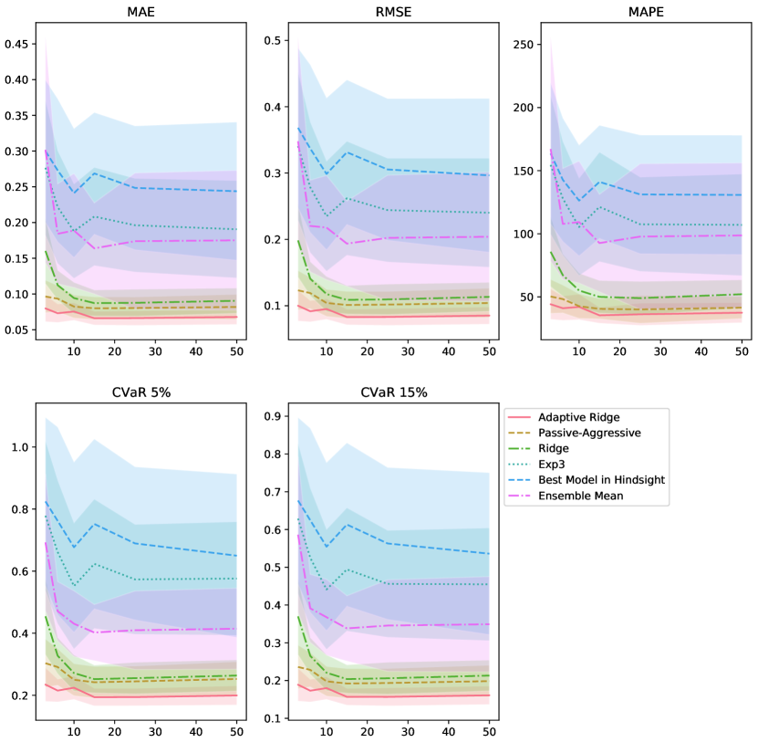
Figure 2: Average performance across 30 seeds of the different ensemble methods with respect to the number of ensemble members. We added in light color the corresponding one-standard deviation intervals around the average.

The results with all metrics in Figure 2 show the same trend. We make the following conclusions:

• The performance increases when more models can be used by the ensemble, which makes sense since there are more opportunities to unveil the underlying ground truth data by learning how the different models make their errors.

• There is a rapid increase in the performance going from 3 ensemble members to 10. However, after 15 ensemble members, the performance is stable and does not improve anymore or becomes slightly worse. It suggests that a high number of forecasters does not necessarily translate to better performance. Instead, a higher number of models can lead to overfitting the training set.

• Adaptive ridge is consistently the best method and outperforms the classic ridge formulation, which is static. The PA model also performs well. These methods clearly outperform the mean baseline and show that a weighted linear combination can significantly improve upon the best model of the ensemble.

• The Exp3 algorithm indeed achieves lower errors than the best model but does not compete with the PA algorithm and the ridge formulations.

4.4 Evaluation of the Ensemble Members’ Drift

These experiments aim to determine how well methods perform when the ensemble members can significantly drift across time.

We fixed the number of ensemble members to $m=10$ and the window size of past forecasts the adaptive part can use to $\tau=5$.

Gaussian Drift

We test several values of $\sigma_{\text{drift}}=s_{\text{drift}}$ ranging from 0 to 1.

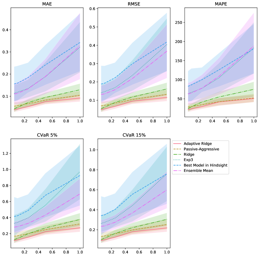
Figure 3: Average performance across 30 seeds of the different ensemble methods with respect to the ensemble members’ possible drift. We added in light color the corresponding one-standard deviation intervals around the average.

Figure 3 shows the following:

• When there is no or very little drift, ridge and adaptive ridge perform very similarly, which is expected since the adaptive part is mainly useful to leverage temporal trends.

• When the ensemble members can drift more than 0.2, ridge starts performing worse than the PA algorithm, which is again expected since the trained weights may differ from the ensemble members’ performance trend on the test set.

• On the other side, adaptive ridge maintains its lead on PA since it can leverage recent trends.

• The baseline methods quickly start to perform terribly with high drift. At the same time, PA and adaptive ridge metrics maintain a seemingly sublinear relationship with respect to the amount of drift possible.

Discrete Gaussian Drift

We also tested the models with a different type of noise, where the Gaussian drift happens or not according to a Bernoulli variable.

For this experiment only, our final forecast values $X_{k}(t)$ of each ensemble member $k\in[m]$ are defined as:

$$X_{k}(t) =\tilde{X}_{k}(t)+b_{k}(t)\cdot\text{drift}_{k}(t),\quad\forall t\in[4000],$$

$$b_{k}(t) \sim\operatorname{Bernoulli}(p_{\text{drift}}),$$

$$\text{drift}_{k}(t) \sim\mathcal{N}(b^{\prime}_{k},\sigma^{\prime}_{k}),$$

where we selected their error biases $b^{\prime}_{1},\ldots b^{\prime}_{m}$ and error standard deviations $\sigma^{\prime}_{1},\ldots,\sigma^{\prime}_{m}$ before hand as:

$$b^{\prime}_{k} \sim\mathcal{N}(0,0.5),$$

$$\sigma^{\prime}_{k} \sim\operatorname{Uniform}(0,0.5).$$

We tested several values of the Bernoulli parameter $p_{\text{drift}}$ ranging from 0 to 1. 0 means no drift is added, and the ensemble members’ errors follow their initial distribution. 1 means the drift is always added, shifting the ensemble members’ errors to a new distribution. Any value in-between means the errors are oscillating between two distributions of errors.

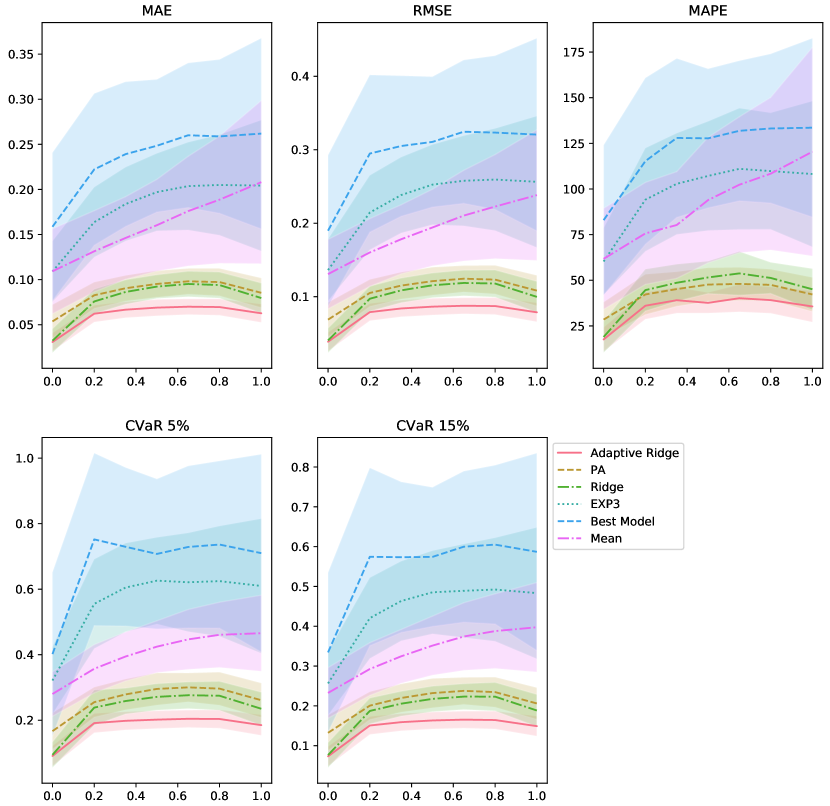
Figure 4: Average performance across 30 seeds of the different ensemble methods with respect to the ensemble members’ possible drift. We added in light color the corresponding one-standard deviation intervals around the average.

The results shown by Figure 4 suggest the following:

• The ridge method cannot compensate for an additional discrete noise as much as the adaptive method.

• Adaptive ridge has the most stable performance across the different regimes, which is expected since it is a robust formulation.

• For all methods, it is more difficult to adjust to oscillating error distributions than to a fixed error distribution, even if the errors are higher in the second distribution.

4.5 Evaluation of the Window of Past Forecasts that Can Be Used

These experiments aim to determine the performance of adaptive ridge with respect to the window size of past forecasts it can use at each time step.

We fixed the number of ensemble members to $m=10$, the drift parameters of the error distributions to $\sigma_{\text{drift}}=0.5,s_{\text{drift}}=0.5$. We vary $\tau\in[1,25]$.

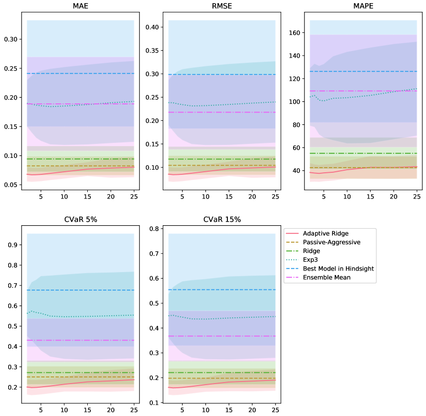
Figure 5: Average performance across 30 seeds of the different ensemble methods with respect to the window size of past data that can be used. We added in light color the corresponding one-standard deviation intervals around the average.

Figure 5 shows the following:

• A large window size deteriorates the performance, as the adaptive ridge model overfits.

• Between a window size of 2 and 8 time steps, the performance is stable. There is a sweet spot around 3-4 past time steps. It suggests the importance of hypertuning this value for the practitioner.

4.6 Evaluation of the Training Data Size

Contrary to all previous experiments, we varied the amount of training and validation data available to evaluate how the different ensemble methods adapt to lower amounts of samples in particular. The test set remained the same as previously for all experiments. We split the training and validation data so that the test set immediately follows those samples. We varied the number of samples between 100 and 3000 by fixing the validation data size to one-third of the data available (e.g., for data size = 750, we get training data size = 500, validation data size = 250).

We fixed the number of ensemble members to $m=10$, the drift parameters of the error distributions to $\sigma_{\text{drift}}=0.5,s_{\text{drift}}=0.5$, and the number of past time steps to use to $\tau=5$.

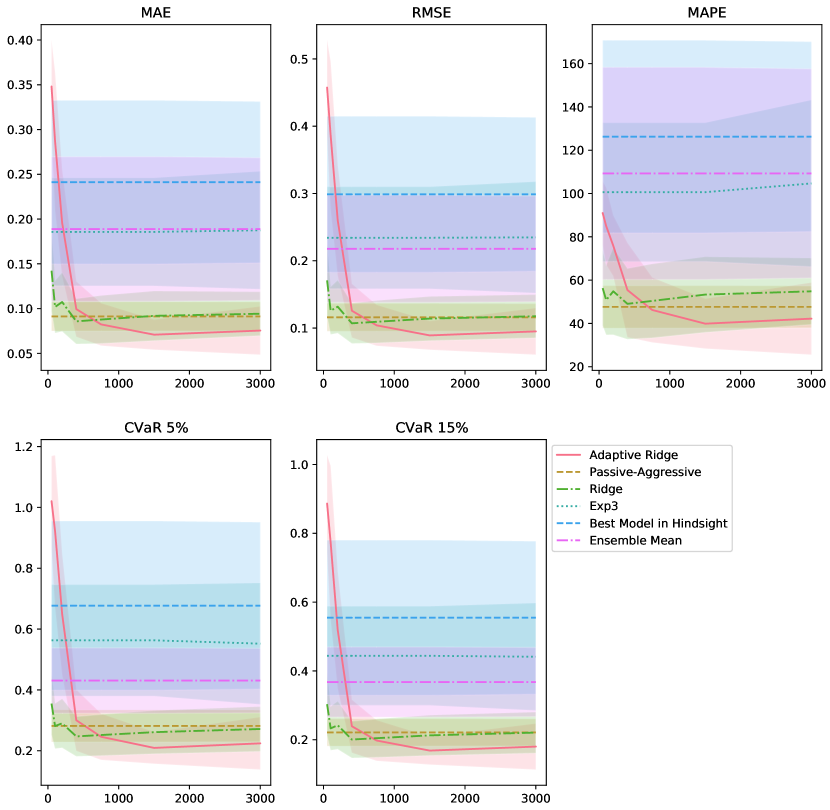
Figure 6: Average performance across 30 seeds of the different ensemble methods with respect to the number of training samples available. We added in light color the corresponding one-standard deviation intervals around the average.

We notice two interesting regimes in Figure 6:

• In the small data regime, with under 500 samples available for training, PA is the best method as it does not rely on any training data. Ridge closely follows and bridges the gap at around 300 samples. The adaptive ridge method suffers from the lack of data as it overfits the training set.

• With more data available, the adaptive ridge method closes the gap at 500 - 750 samples and then outperforms all other methods.

• After 750 samples, the performance of all methods remains stable, with adaptive ridge being the best, followed by PA, and then ridge.

These experiments highlight that the adaptive framework is primarily suitable when sufficient data is available to determine adaptive coefficients that generalize well enough.

4.7 Conclusion of the Synthetic Experiments

We summarize our main findings:

• Adaptive ridge has a significant edge over ridge when sufficient data is available and when ensemble members may suffer from performance drift.

• Adaptive ridge is not suitable when there is little data available. In that case, a purely online method such as PA should be preferred, or a simpler static method such as ridge.

• We highlight the importance of validating the different hyperparameters of the adaptive ridge method: the regularization factor $\lambda$ and the window size $\tau$ of past forecasts to use in the adaptive term. Adaptive ridge, due to its additional variables, may be sensitive to overfitting in certain situations (e.g., large window size, small training data size).

• Ensemble methods such as the Ensemble Mean and Exp3 sum models’ weights to 1, while ridge and adaptive ridge can correct forecast biases with negative weights offering greater accuracy and robustness than the best model in hindsight.

5 Real-World Case Studies

This section illustrates the benefits of our adaptive ensemble method with real-world data. We investigate three different applications where the time series characteristics differ (see Figure 7):

1. Air pollution management through wind speed forecasting: the time series exhibits a daily cyclical behavior and a long-term seasonality.

2. Energy use forecasting: the time series exhibits bursts a few hours a week.

3. Tropical cyclone intensity forecasting: the time series are shorter and smoother, but the underlying system is chaotic and complicated to predict.

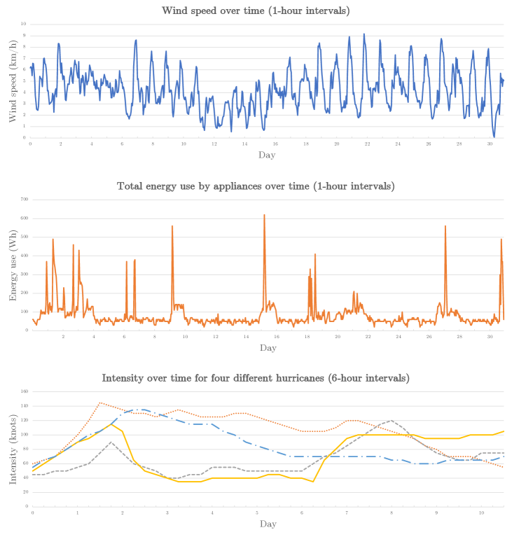
Figure 7: Subsamples of the time series for our three real-world use cases: wind speed at Safi factories, energy use by appliances, tropical cyclone intensity.

5.1 Next-Hour Wind Speed Forecasting for Pollution Management

Motivation

Air pollution is a pressing concern with far-reaching consequences for human health, the environment, and ecosystems. The emission of toxic substances from chemical factories poses a significant risk to nearby populations, mainly when meteorological conditions carry the pollution toward populated areas. It is crucial to accurately predict weather conditions to inform real-time, effective pollution management strategies to mitigate this risk. This forms the basis of our first use case: predicting wind speed for air pollution management. Our data comes from a phosphate production site in Morocco, the largest chemical industry plant in the country. Previously, Bertsimas et al. (2023) demonstrated with this plant the effectiveness of a data-driven approach, including a weighted average ensemble model, in reducing the diffusion of air pollution from industrial plants into nearby cities, providing a valuable use case to show how our adaptive ensembles can improve further the robustness and accuracy.

Air Pollution Management Pipeline

The phosphate production site is located 10km southwest of Safi city, Morocco, threatening the health and well-being of the 300,000 residents. With this population in close proximity, weather conditions play a critical role in determining air pollution dispersion. The site therefore implemented a comprehensive monitoring procedure that includes planning production rates and shutdowns based on 48-hour meteorological forecasts, as well as real-time wind monitoring systems to detect dangerous conditions and stop production. The timely and accurate wind speed prediction in the next hour is crucial for the effective functioning of this procedure.

Building on the success of Bertsimas et al. (2023)’s implementation of regularized linear regression models for wind speed forecasting, we explore the potential of the adaptive ridge method to improve the accuracy and robustness and enhance the pollution management pipeline.

5.1.1 Data

Ensemble Members

The Safi operations team receives the local official weather forecast bulletins from the Moroccan weather agency daily around 6:00 am GMT, with an update around 6:00 pm GMT. The wind speed forecasts are provided hourly for the next 48 hours. Besides this operational forecast, the different models used by Bertsimas et al. (2023) are XGBoost, Decision Trees, Optimal Regression Trees, Lasso Regression, and Ridge Regression. These models took as input the recent meteorological data observations.

We have access to the 8494 historical one-hour lead time wind speed forecasts made by these 6 models between 2019 and 2022 for every hour. The ground truth was measured by a sensor on-site that collected data every minute and then was averaged hourly on the Safi platforms.

Experiments Protocol

We split the data chronologically into training (50%), validation (20%), and test (30%) sets. We standardized all data (targets and features) by subtracting the mean of the training targets and dividing by the standard deviation of the training targets.

After selecting the best hyperparameter combination for each ensemble method using the validation set (see the Appendix for more details), we retrained the models on the training and validation sets combined. We then evaluated them on the test set in the same way we conducted the synthetic experiments.

5.1.2 Results

Table 2 compares the performance of the different ensemble methods with the same metrics described previously.

Adaptive ridge consistently provides the best performance across all metrics, improving over the best model in hindsight by 8% in MAE, 17% in RMSE, 7% in MAPE, 26% in CVaR 5%, and 14% in CVaR 15%. The adaptive ridge can substantially reduce the worst-case errors, which is critical for the success of the pollution management pipeline.

In comparison, the other ensemble methods fail to outperform the best model in hindsight consistently. As expected, Exp3 provides comparable performance to the best model in hindsight: 0.510 vs. 0.507 in MAE, 0.690 vs. 0.756 in RMSE, and more robust results: 1.87 vs. 2.27 in CVaR 5%, 1.36 vs. 1.46 in CVaR 15%.

Adaptive ridge outperforms ridge substantially on all metrics, notably the robustness, by 17% in CVaR 5% and 12% in CVaR 15%, which is of substantial interest to the plant operators to prepare better against incoming dangerous weather conditions.

Table 2: Results for each metric and ensemble method on the test set for the wind speed forecasting task on the Safi site. Results are given in km/h.

Ensemble Method	MAE	RMSE	MAPE (%)	CVaR 5%	CVaR 15%
Best Model in Hindsight	$0.507$	$0.756$	$15.9$	$2.27$	$1.46$
Ensemble Mean	$0.553$	$0.783$	$17.4$	$2.27$	$1.52$
Exp3	$0.510$	$0.690$	$16.5$	$1.87$	$1.36$
Passive-Aggressive	$0.643$	$0.868$	$20.1$	$2.35$	$1.72$
Ridge	$0.521$	$0.718$	$16.7$	$2.03$	$1.42$
Adaptive Ridge	0.469	0.626	14.8	1.68	1.25

5.1.3 Remarks on the adaptive coefficients

The ability of regression coefficients to adapt over time is demonstrated in Figure 8, which plots a subset of these values over a period of two weeks. The rate of change for the coefficients varies among models, with some displaying more significant shifts than others. Furthermore, as depicted in Figure 9, the coefficients can take on both positive and negative values. A daily cyclical pattern is also observed, which aligns with the cyclical nature of the forecast errors (due itself to the cyclical nature of the weather data).

It is worth noting that the predictions of some models may compensate for one another, particularly when there is a high degree of correlation among them. In such cases, practitioners may want to consider selecting a subset of models before utilizing an adaptive ensemble, and potentially impose an additional constraint that the sum of their coefficients is equal to 1, depending on the specific application.

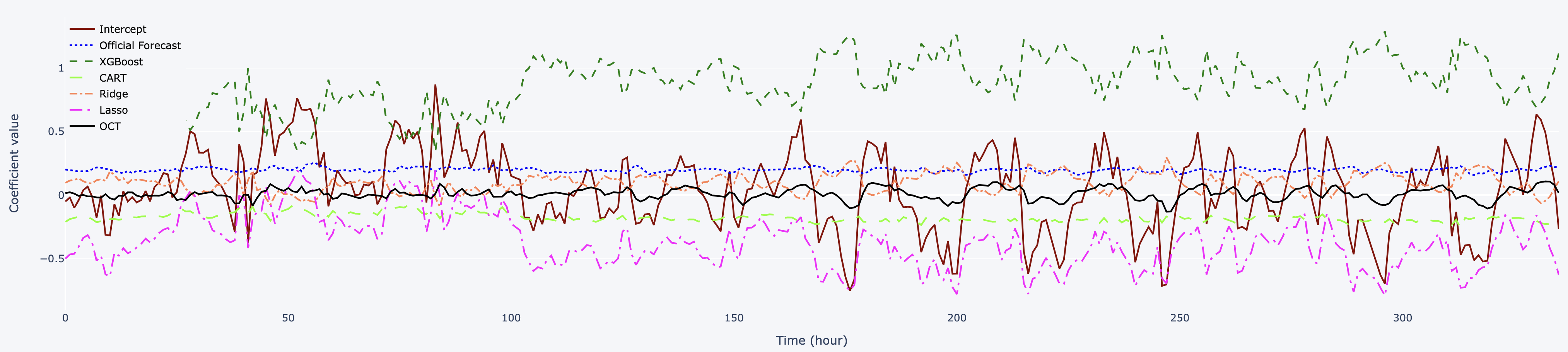
Figure 8: Evolution every hour of the regression coefficients values for each ensemble member.

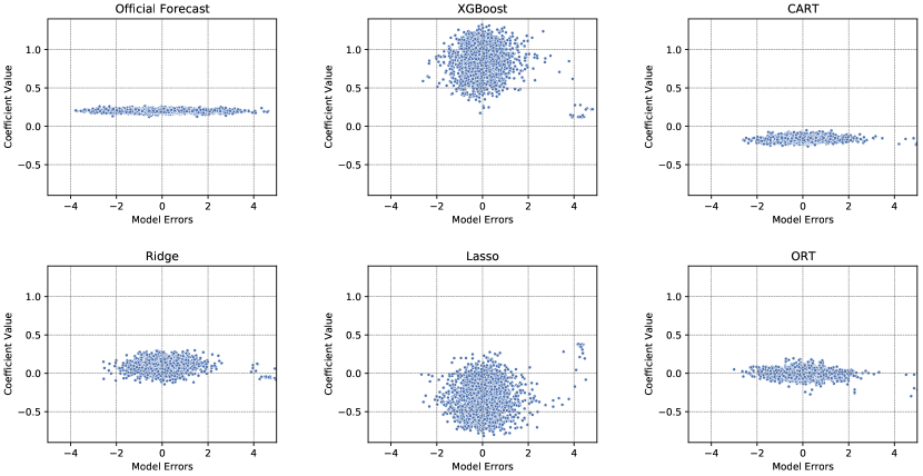
Figure 9: Coefficient values of each ensemble member with respect to their errors.

5.2 Energy Consumption Forecasting

Due to fast urbanization, rising population, and increased social needs, the energy demand in the building sector has expanded dramatically over the past few decades. In particular, appliances in residential buildings represent a substantial part of the electrical energy demand, approximating 30% (EIA, 2022). Numerous studies investigated appliances’ energy use in buildings and developed forecasting models of electrical energy consumption in buildings to guide multiple applications such as detecting abnormal energy use patterns, determining adequate sizing of alternate energy sources and energy storage to diminish power flow into the grid, informing energy management system for load control, demand-side management and demand-side response, predicting electricity price (e.g., Pham et al. (2020); Olu-Ajayi et al. (2022); Zaffran et al. (2022)). According to Colmenar-Santos et al. (2013), the availability of a building energy system with precise forecasting could save between 10% and 30% of all energy consumed. Overall, as accurate and robust forecasting can be impactful, we investigate how adaptive ridge compares with the other ensemble techniques using real-world data on appliance energy consumption provided by Candanedo et al. (2017).

5.2.1 Data

The dataset is publicly available at the University of California Irvine (UCI) Machine Learning repository. First, we trained and selected our own forecasting models to constitute the ensemble members before comparing the different ensemble methods.

Each observation in the dataset is a vector of measurements made by a wireless sensor network in a low-energy building. The predictive features we use include the temperature and humidity conditions in various rooms in the building, the weather conditions in the nearest weather station, and the date and time. Our goal is to predict the total energy consumption in Wh of the building’s appliances within one hour at each time step. Measurements are taken every 10 minutes over 4.5 months. We aggregated the current features with the past 5 time steps of data for each forecasting case to form a vector of 168 features used as predictors for standard machine learning models. We trained several forecasting models that will constitute our ensemble members. We separated the data chronologically into a training set (50%, 9858 samples), validation set 1 (25%, 4929 samples), validation set 2 (10%, 1973 samples), and test set (15%, 2956 samples).

We used the Python package Lazy Predict to conveniently train and cross-validate 36 different forecasting models using the training set only. Models trained included numerous tree-based models, linear regressions, support vector machines, neural networks, and various other methods. Among the 30 models trained, we selected the best 10 with respect to MAE on the validation set 1 to constitute our final ensemble members. The best 10 models were Ordinary Least Squares (OLS), Ridge, Bayesian Ridge, ElasticNet, Huber Regressor, Least Angle Regression (LARS), Lasso, LassoLARS, Linear Support Vector Regression, and Orthogonal Matching Pursuit.

We collected the predictions of these different models on the validation sets and test sets and used validation set 1 as training data for the ensembles, validation set 2 as validation data for the ensembles, and the test set to evaluate the results.

5.2.2 Results

The results presented in Table 3 demonstrate the superiority of the adaptive ridge method compared to other ensemble techniques. It is the only ensemble method that outperformed the best model in hindsight in MAE and RMSE, showing a 15% improvement in MAE and a 26% improvement in RMSE. The MAPE performance of adaptive ridge was similar to the best ensemble member in hindsight (23.5% vs. 23.2%), while the second-best ensemble method, Exp3, achieved a MAPE of 27.6%.

The energy consumption target values in this dataset displayed significant bursts, as shown previously in Figure 7, making it difficult for all ensemble methods to accurately capture such events, as evidenced by the poor CVaR scores. However, the adaptive ridge method demonstrated its ability to effectively leverage the errors of each ensemble member, resulting in more robust solutions than any other method. The improvement in CVaR 5% was 27% and 28% in CVaR 15% compared to the best ensemble member, while ridge showed an improvement of 7% in CVaR 5% and 8% in CVaR 15%.

Table 3: Results for each metric and ensemble method on the test set for the energy consumption task. Results are given in Wh.

Ensemble Method	MAE	RMSE	MAPE (%)	CVaR 5%	CVaR 15%
Best Model in Hindsight	$31.1$	$80.0$	$\mathbf{23.2}$	$309.0$	$158.3$
Ensemble Mean	$33.3$	$79.4$	$27.6$	$304.3$	$157.6$
Exp3	$32.9$	$78.8$	$27.1$	$301.9$	$156.4$
Passive-Aggressive	$52.2$	$149.1$	$45.0$	$476.7$	$249.8$
Ridge	$35.3$	$76.4$	$33.7$	$287.5$	$145.0$
Adaptive Ridge	$\mathbf{26.3}$	59.4	$23.5$	$\mathbf{224.9}$	$\mathbf{113.8}$

5.3 Tropical Cyclone Intensity Forecasting

Motivation

Tropical cyclones are a considerable threat to communities, causing hundreds of deaths and billions of dollars in damage each year. The US National Hurricane Center (NHC) forecasts tropical cyclones’ track, intensity, size, structure, storm surges, rainfall, and tornadoes. Intensity predictions, i.e., the maximum sustained wind speed of a storm over a 1-minute interval, is one of the most important and difficult characteristics to forecast and directly impacts decision-making. In this real-world use case, we evaluate the effectiveness of the different ensemble methods for 24-hour lead time tropical cyclone intensity forecasting, which is critical to undertake life-saving measures and mitigate the impact of these devastating natural disasters.

Background on the Ensemble Members

Current operational TC forecasts used by the NHC can be classified into dynamical models, statistical models, and statistical-dynamical models (Cangialosi, 2020). Dynamical models, also known as numerical models, utilize powerful supercomputers to simulate atmospheric fields’ evolution using dynamical and thermodynamical equations (Biswas et al., 2018; ECWMF, 2019). Statistical models approximate historical relationships between storm behavior and storm-specific features and, in general, do not explicitly consider the physical process (Aberson, 1998; Knaff et al., 2003). Statistical-dynamical models use statistical techniques but further include atmospheric variables provided by dynamical models (DeMaria et al., 2005). Lastly, the NHC employs consensus models (i.e., ensemble models) to combine individual operational forecasts (Cangialosi, 2020; Cangialosi et al., 2020). In addition, recent developments in deep learning enabled machine learning models to employ multiple data processing techniques to process and combine information from a wide range of sources and create sophisticated architectures to model spatial-temporal relationships. In particular, Boussioux et al. (2022) proposed a deep feature extractor methodology combined with boosted tree methods that have comparable performance with operational forecasts.

5.3.1 Data

We collected the different operational and machine learning intensity forecasts provided by Boussioux et al. (2022). We used the forecasts made on their test set, corresponding to the years 2016-2019. They obtained operational forecast data from the Automated Tropical Cyclone Forecasting (ATCF) data set maintained by the NHC (Sampson and Schrader, 2000; National Hurricane Center, 2021). The ATCF data contains historical forecasts by operational models used by the NHC for its official forecasting of tropical and subtropical cyclones in the North Atlantic and Eastern Pacific basins.

Table 4 lists the 7 forecast models included as ensemble members and the 2 operational benchmark models and summarizes the predictive methodologies employed.

Overall, our ensemble members comprise four deep learning models (Hurricast), one statistical-dynamical model (Decay-SHIPS), and two dynamical models (GFSO, HWRF). We benchmark our ensemble methods against the forecasts made by FSSE and OFCL, which are the highest-performing consensus models used by the NHC. The technical details of all the models can be found in Cangialosi (2020) and Boussioux et al. (2022).

Table 4: Summary of all tropical cyclone intensity forecasting models used as ensemble members or benchmark.

$\begin{array}[]{|l|l|l|l|}\hline\cr\text{ {Model ID} }&\text{ {Model name} }&\text{ {Model type} }&\text{ {Used as} }\\ \hline\cr\text{ HUML-(stat, xgb) }&\text{ Hurricast (tabular data) }&\text{ Gradient-boosted trees }&\text{ Ensemble member }\\ \text{ HUML-(stat/viz, xgb/td) }&\text{ Hurricast (tabular and vision data) }&\text{ Feature extraction with tensor decomposition }&\text{ Ensemble member }\\ &&\quad\text{+ Gradient-boosted trees}&\\ \text{ HUML-(stat/viz, xgb/cnn/gru) }&\text{ Hurricast (tabular and vision data) }&\text{ Feature extraction with deep learning }&\text{ Ensemble member }\\ &&\quad\text{(CNN, GRU) + Gradient-boosted trees }&\\ \text{ HUML-(stat/viz, xgb/cnn/transfo) }&\text{ Hurricast (tabular and vision data) }&\text{ Feature extraction with deep learning}&\text{ Ensemble member }\\ &&\quad\text{(CNN, Transformers) + Gradient-boosted trees }&\\ \hline\cr\text{ Decay-SHIPS }&\text{ Decay Statistical Hurricane Intensity }&\text{ Statistical-dynamical }&\text{ Ensemble member }\\ &\quad\text{ Prediction Scheme }&&\\ \text{ GFSO }&\text{ Global Forecast System model }&\text{ Multi-layer global dynamical }&\text{ Ensemble member }\\ \text{ HWRF }&\text{ Hurricane Weather Research and }&\text{ Multi-layer regional dynamical }&\text{ Ensemble member }\\ &\quad\text{ Forecasting model }&&\\ \hline\cr\text{ FSSE }&\text{ Florida State Super Ensemble }&\text{ Corrected consensus }&\text{ Benchmark model }\\ \text{ OFCL }&\text{ Official NHC Forecast }&\text{ Consensus }&\text{ Benchmark model }\\ \hline\cr\end{array}$

5.3.2 Experiments Protocol

Implementation Adjustments

The use-case of tropical cyclone intensity forecasting requires two minor implementation adjustments. First, since we use the different forecasts for lead time 24-hour every 6 hours, this means at a time step $t$ we don’t predict $t+1$, but rather $t+4$ ($t+24h$ instead of $t+6h$). Therefore, for all methods, we only use the ground truth data that would be available in real-time to update the weights, i.e., to predict $t+4$, we do not use the information that becomes available at $t+1,t+2,t+3$.

Second, tropical cyclones are temporary events: the forecast data comes as several time series of different lengths instead of only one. For the adaptive ridge method, we treat all samples from each hurricane as independent samples in the training set and we build $\mathbf{Z}_{t}$ as usual. For the bandit and PA method, for each new tropical cyclone, we reuse the latest updated weights computed on the previous tropical cyclone.

Training, Validation, Test Splits

The forecast data comprises 870 samples for the North Atlantic Basin and 849 for the Eastern Pacific basin. We split the data chronologically into training (50% of the data), validation (20% of the data), and test (30% of the data) sets.

5.3.3 Results

Table 5 compares the different ensemble methods. The adaptive ridge and ridge methods outperform all other ensembles, including the current operational models OFCL and FSSE, which is of significant interest for operational use due to its potential to improve the official forecasts issued by the NHC. In particular, the good performance of adaptive ridge in terms of CVaR is particularly relevant for tropical cyclone forecasting as it may decrease the worst errors, which are the ones leading to poor decision-making on the ground. For instance, adaptive ridge outperforms the official forecast OFCL by 5% (resp. 21%) on the North Atlantic (resp. Eastern Pacific) basin in CVaR 15% and by 12% (resp. 17%) in MAE.

The Ensemble Mean and Exp3 methods perform similarly to the operational consensus FSSE and OFCL and generally improve slightly over the best model in hindsight. Adaptive ridge has the best performance overall across basins and metrics, with only ridge slightly surpassing it in CVaR on the North Atlantic basin. The adaptive component provides a valuable performance boost compared to ridge only, such as an MAE gain of 4% on the North Atlantic basin and 9% on the Eastern Pacific basin.

Table 5: Results in knots for each metric and ensemble method for 24-hour lead time intensity forecasting task. Bold values highlight the best performance for each metric.

	North Atlantic Basin					Eastern Pacific Basin
Ensemble Method	Comparison on 261 cases					Comparison on 254 cases
	MAE	RMSE	MAPE (%)	CVaR 5%	CVar 15%	MAE	RMSE	MAPE (%)	CVaR 5%	CVaR 15%
Best Model in Hindsight	9.2	12.2	14.2	31.4	24.6	11.3	15.3	14.5	41.1	30.8
Ensemble Mean	9.4	12.8	14.0	35.2	25.6	10.9	14.6	14.2	38.2	29.2
Exp3	8.8	11.5	13.3	30.0	22.6	10.3	14.9	15.5	43.3	31.1
Passive-Aggressive	9.1	12.4	13.9	34.6	25.3	17.9	22.9	27.1	57.2	44.4
FSSE	8.8	11.6	13.8	31.0	23.2	10.0	14.4	15.5	41.3	28.9
OFCL	8.4	11.4	13.3	29.8	22.2	10.6	15.6	17.2	44.3	30.6
Ridge	7.7	10.3	11.7	27.2	21.0	9.7	13.6	15.0	39.2	27.8
Adaptive Ridge	7.4	10.2	11.6	28.6	21.1	8.8	12.1	13.4	34.1	24.1

5.4 Further Applications to Adaptive Feature Selection

Beyond ensemble modeling, our methodology can be employed for adaptive feature selection in complex multimodal tasks. For instance, in healthcare, the methods developed by Soenksen et al. (2022); Bertsimas et al. (2022) merge modalities such as tables, text, time series, and tables by extracting features through deep learning, forming a unified vector representation. This vector is then employed to generate forecasts using standard machine-learning algorithms. However, the weighting of these features remains static over time. We can dynamically identify the most relevant features for predicting patient outcomes, disease progression, or treatment responses by incorporating adaptive feature selection. Additional applications of adaptive multimodal feature selection encompass natural disaster management (Zeng and Bertsimas, 2023), climate change, agriculture, finance and economics, and many others.

6 Conclusion

Using an ARO approach, this paper presented a novel methodology for building robust ensembles of time series forecasting models. Our technique is based on a linear ensemble framework, where the weights of the ensemble members are adaptively adjusted over time based on the latest errors. This approach robustly adapts to model drift using an affine decision rule and a min-max problem formulation transformed into a tractable form with equivalence theorems.

We have demonstrated the effectiveness of our adaptive ensemble mechanism through a series of synthetic and real-world experiments. Our results have shown that our approach outperforms several standard ensemble methods in terms of accuracy and robustness. We have also applied our technique to three real-world use cases – weather forecasting for air pollution management, energy consumption forecasting, and tropical cyclone intensity forecasting – highlighting its merit for critical tasks where robustness and risk minimization are critical.

One of the advantages of our method is that it relies on a robust linear formulation, which makes it valuable from a practical standpoint for ease of deployment and interpretability. However, this method also requires the availability of a training set of some size, a trade-off we exhibited with synthetic experiments. Therefore, we recommend using our adaptive ensemble framework when a few hundred historical time series points are available for training.

Adaptive ensembles have the potential for many time series applications, including epidemiological predictions, healthcare operations, logistics, supply chain, manufacturing, finance, and product demand forecasting.

A Additional Details on Data Experiments

A.1 Evaluation of the Training Time with Synthetic Data

We provide the computational time of adaptive ridge when we vary the training data size (Table 6), the number of past time steps to use for the adaptive rule (Table 7), and the number of ensemble members available (Table 8). Overall, the method remains tractable with typical values of those hyperparameters.

Table 6: Average training time across 30 seeds of adaptive ridge with respect to the number of samples used in the training set, when we fix the number of ensemble members to $m=10$ and the number of past time steps to use to $\tau=5$.

Number of samples in training set Average time (s)

100 $$0.4$$

200

400

750 64

1500 92

3000 239

Table 7: Average training time across 30 seeds of adaptive ridge with respect to the number of past time steps to use, when we fix the number of ensemble members to $m=10$ and the number of training samples to $N=3000$.

$$\begin{array}[]{|c|c|}\hline\cr\textbf{ Number of time steps }&\textbf{ Average time (s) }\\ \hline\cr 2&54\\ 3&100\\ 5&239\\ 10&603\\ 15&1079\\ 25&1361\\ \hline\cr\end{array}$$

Table 8: Average training time across 30 seeds of adaptive ridge with respect to the number of ensemble members to use, when we fix the number of past time steps to $\tau=5$ and the number of training samples to $N=3000$.

$$\begin{array}[]{|c|c|}\hline\cr\text{ {Number of ensemble members} }&\text{ {Average time} (s) }\\ \hline\cr 3&7\\ 6&51\\ 10&239\\ 15&236\\ 25&236\\ 50&250\\ \hline\cr\end{array}$$

A.2 Hyperparameter Tuning in Real-World Experiments

For all real-world experiments, we tuned the following hyperparameters:

• regularization factor for Ridge, Adaptive Ridge, and Passive-Aggressive with the values $\lambda,\epsilon_{PA}\in\{0,1e-4,1e-3,1e-2,1e-1,1,2\}$

• window size of past data to use: $\tau\in[1,10]$.

A.3 Synthetic Data Hyperparameters

Table 9 summarizes the different hyperparameters involved in our synthetic experiments.

Table 9: List of features included in our statistical data with their fixed value or range when they vary.

References

- Aberson (1998) Sim D. Aberson. Five-day tropical cyclone track forecasts in the north atlantic basin. Weather and Forecasting, 13(4):1005 – 1015, 1998.
- Adhikari and Agrawal (2012) Ratnadip Adhikari and R. K. Agrawal. Combining multiple time series models through a robust weighted mechanism. In 2012 1st International Conference on Recent Advances in Information Technology (RAIT), pages 455–460, 2012. doi: 10.1109/RAIT.2012.6194621.
- Bates and Granger (1969) J. M. Bates and C. W. J. Granger. The combination of forecasts. OR, 20(4):451–468, 1969.
- Ben-Tal et al. (2004) A. Ben-Tal, A. Goryashko, E. Guslitzer, and A. Nemirovski. Adjustable robust solutions of uncertain linear programs. Mathematical Programming, 99(2):351–376, 2004.
- Bennouna and Van Parys (2022) Amine Bennouna and Bart Van Parys. Holistic robust data-driven decisions, 2022. URL https://arxiv.org/abs/2207.09560.