Dynamics for Super-Extremal Kerr Binary Systems at ${\cal O}(G^{2})$

Abstract

Using the recently derived higher spin gravitational Compton amplitude from low-energy analytically continued ($a/Gm\gg 1$) solutions of the Teukolsky equation for the scattering of a gravitational wave off the Kerr black hole, observables for non-radiating super-extremal Kerr binary systems at second post-Minkowskian (PM) order and up to sixth order in spin are computed. The relevant 2PM amplitude is obtained from the triangle-leading singularity in conjunction with a generalization of the holomorphic classical limit for massive particles with spin oriented in generic directions. Explicit results for the 2PM eikonal phase written for both Covariant and Canonical spin supplementary conditions – CovSSC and CanSSC respectively – as well as the 2PM linear impulses and individual spin kicks in the CanSSC are presented. The observables reported in this letter are expressed in terms of generic contact deformations of the gravitational Compton amplitude, which can then be specialized to Teukolsky solutions. In the latter case, the resulting 2PM observables break the newly proposed spin-shift symmetry of the 2PM amplitude starting at the fifth order in spin. Aligned spin checks as well as the high energy behavior of the computed observables are discussed.

Introduction. The application of QFT-inspired methods to compute observables in classical gravity has seen tremendous advances in the last years Cheung et al. (2018); Kosower et al. (2019); Bern et al. (2022a, b, 2021, 2020, 2019); Dlapa et al. (2023, 2022); Kälin et al. (2020); Mogull et al. (2021); Jakobsen et al. (2022a); Elkhidir et al. (2023); Brandhuber et al. (2023); Herderschee et al. (2023); Georgoudis et al. (2023); Di Vecchia et al. (2021) due to their potential relevance for analyzing measured signals in gravitational wave (GW) detectors Abbott et al. (2016). The use of these techniques is justified by the separation of scales that allows to treat physics problems in an effective manner. For instance, an isolated black hole (BH) seen from far away can be thought of as a point particle, and its finite size effects such as spin multipole moments can be modeled by effective operators in (classical) EFT constructions Levi and Steinhoff (2015); Bern et al. (2022c); Chung et al. (2020a); Jakobsen and Mogull (2022a); Liu et al. (2021); Arkani-Hamed et al. (2017); Chung et al. (2019); Bautista et al. (2022); Aoude et al. (2022a, b). These operators are accompanied by free coefficients parametrizing the UV ignorance of the effective model; they can be fixed by matching computations in the effective and the full theory. Following this logic, an astonishingly simple description of an isolated linearized Kerr BH Vines (2018) – effectively a super-extremal (SE) Kerr BH with spin parameter $a^{\star}=\frac{a}{Gm}\gg 1$, where $m$ and $a$ are its mass and ring radius respectively – as an elementary particle of infinite spin minimally coupled to gravity, has recently appeared in the literature Guevara et al. (2019); Chung et al. (2019); Arkani-Hamed et al. (2019); Aoude et al. (2020).

Actual Kerr BHs are however neither isolated objects in nature nor linearized solutions of the field equations as they possess spin parameters satisfying $a^{\star}\leq 1$. A correct description of these objects requires therefore resummations of the perturbative computations. Accomplishing these resummations from a perturbative amplitude approach is a heroic task not yet addressed along these lines of reasoning, and therefore relying on the effective one-body formalism Buonanno and Damour (1999, 2000); Damour (2001); Vines (2018); Buonanno et al. (2006); Khalil et al. (2023), as an alternative way to study these more realistic Kerr BHs scenarios . Nevertheless, perturbative approaches are still very useful to gain insights into the physics of actual Kerr BH systems, and in this work, we follow these lines to study systems made not of actual Kerr BHs, but of their close relatives, SE Kerr BHs (fastly rotating objects).

Although SE Kerr BHs are not real objects in nature, they share many features of actual Kerr BHs, as the two are related via analytic continuation of the spin parameter from the physical region $a^{\star}\leq 1$, to the SE $a^{\star}\gg 1$ region. For observables that cannot probe the nature of the BH horizon – which we shall refer to as true conservative observables – this continuation should not possess any subtlety and their values computed for one kind of objects or the others should coincide in the overlapping (continuation) region . In this sense, SE Kerr observables readily encapsulate part of the dynamic for actual Kerr BHs Vines (2018); Bini and Damour (2017); Chung et al. (2020a); Bern et al. (2020); Kosmopoulos and Luna (2021); Chen et al. (2022); Jakobsen and Mogull (2022a); Levi and Steinhoff (2021, 2015); Levi and Yin (2022); Kim et al. (2022a); Liu et al. (2021); Jakobsen and Mogull (2022a); Goldberger et al. (2018); Jakobsen et al. (2022b, c, a); Jakobsen and Mogull (2022b); Febres Cordero et al. (2022); Blanchet (2014); Porto (2016); Levi (2018); Levi and Steinhoff (2016, 2021); Levi et al. (2020a); Antonelli et al. (2020a); Levi et al. (2020b); Antonelli et al. (2020b); Kim et al. (2021); Levi et al. (2021); Levi and Teng (2021); Maia et al. (2017); Cho et al. (2022, 2021); Kim et al. (2022a, b); Levi et al. (2022); Levi and Yin (2022). Observables that can probe the nature of the BH horizon – absorptive observables accounting for fluxes of energy at the BH horizon – are more subtle since the notion of absorption does not exist for objects without a horizon; hence, SE Kerr BH observables look always conservative. These can however receive contributions from effective operators that mimic the physical effects happening at the horizon of an actual Kerr BH, but whose definite identification requires comparison to alternative approaches to study absorptive effects Tagoshi et al. (1997); Poisson (2004); Chatziioannou et al. (2013, 2016); Isoyama and Nakano (2018); Goldberger and Rothstein (2006); Goldberger et al. (2020); Porto (2008); Saketh et al. (2022, 2022).

In this work, we compute conservative observables for the scattering of two SE Kerr BHs at $\mathcal{O}(G^{2})$, but whose content can potentially encode true conservative as well as absorptive effects for actual Kerr BHs. For this, we use the recently extracted higher spin gravitational Compton amplitude from low-energy solutions of the Teukolsky equation in the SE region Bautista et al. (2022). The observables of interest in this work are the linear impulse and the individual spin kicks, for generic spin orientations. We will use the eikonal phase as an intermediate object, and compute the observables using formula (15), proposed by the authors of references Bern et al. (2020); Kosmopoulos and Luna (2021). Since contact deformation of the Compton amplitude enters the 2PM amplitude only through the triangle diagrams (fig. 1), we expect this formula (15) (showed to be valid for orders $a^{n\leq 4}$ at 2PM Bern et al. (2020); Kosmopoulos and Luna (2021); Chen et al. (2022)) to continue to be valid for higher spin orders.

A tree-level gravitational Compton amplitude from the Teukolsky equation. In Bautista et al. (2022), an ansatz for the $\mathcal{O}(G)$ opposite helicity, higher spin gravitational Compton amplitude of the form (momentum cons. $p_{4}=p_{1}+k_{2}+k_{3}$)

$$A_{4}^{(S)}=A_{4}^{0}\left(e^{(2w+k_{3}-k_{2})\cdot a}{+}P_{\xi}(k_{2}\cdot a,{-}k_{3}\cdot a,w\cdot a)\right)_{2S}\,,$$ (1)

was written invoking physical constraints such as locality, unitarity, 3-point factorization,and crossing symmetry, together with a prescription to write contact deformations – capture by $P_{\xi}$ – that match Teukolsky solutions only in a non-trivial manner .

The scalar contribution, $A_{4}^{0}$ in (1), encodes the helicity and physical pole structure of the amplitude, whereas the terms inside the big parenthesis are only functions of the kinematic invariants and the spin of the massive legs. Explicitly, the former reads

$$A_{4}^{0}=32\pi Gm^{2}\frac{(\epsilon_{2}\cdot u)^{2}(\tilde{\epsilon}_{3}\cdot u)^{2}}{\xi},\,\,\,\xi=\frac{(s-m^{2})^{2}}{m^{2}t}\,,$$ (2)

which we choose to evaluate in the gauge

$$\epsilon_{2}=\frac{\sqrt{2}|3]\langle 2|}{[32]}\propto\tilde{\epsilon}_{3}=\frac{\sqrt{2}|3]\langle 2|}{\langle 32\rangle}\,,\,\,\,w^{\mu}:=\frac{u\cdot k_{2}}{u\cdot\epsilon_{2}}\epsilon^{\mu}_{2}\,.$$ (3)

Here we have included the massless vector $w^{\mu}$ entering in (1), which is constructed from the spinors of the massless legs, and $u=p_{1}/m$, is the incoming massive leg’s four-velocity, with $m$ its respective mass.

The function $P_{\xi}$ contains contact deformations of the BCFW exponential – some of which at the same time cure the unphysical singularities that appear starting at $\mathcal{O}(a^{5})$ when the exponential function is expanded – was written as a Laurent expansion in the optical parameter $\xi$, having the explicit form given in (B). This expansion was further parametrized by three multi-variable polynomials $p^{(m)}_{|a|},q^{(m)}_{|a|},r^{(m)}_{|a|}$, functions of $(k_{2}\cdot a,-k_{3}\cdot a,w\cdot a)$, symmetric in their first two arguments, but also including a linear correction in $\omega|a|$, with $\omega\approx(s-m^{2})/2m$, the energy of the massless legs. Up to the sixth order in spin, these polynomials have the explicit form given by eqs. (28-29), and contain two type of spin operators: regular operators, functions of only $\mathcal{R}=\{k_{2}\cdot a,k_{3}\cdot a,w\cdot a\}$, and exotic operators, functions of $\mathcal{R}\cup\{\omega|a|\}$. The former will encapsulate the real contributions (at the level of the phase shift) to the solution to the Teukolsky equation, whereas the latter accounts for contributions that are imaginary when the BH rotation parameter satisfies the inequality $a^{\star}\leq 1$.

Each effective operator in $p^{(m)}_{|a|},q^{(m)}_{|a|},r^{(m)}_{|a|}$ is accompanied by a free coefficient $c_{i}^{(j)},d_{i}^{(j)},f_{i}^{(j)}$ respectively; contact deformations were shown to appear starting at fourth order in spin as known from the work Chung et al. (2019). These free coefficients were further fixed by requiring that (1) matches the $\mathcal{O}(G)$ sector of the low energy limit ($\epsilon=Gm\omega\ll 1$) of the scattering amplitude for the scattering of a GW off the Kerr BH, computed with the tools of black hole perturbation theory Sasaki and Tagoshi (2003); Bautista et al. (2021). Explicit solutions up to six order in spin can be found in Table 1 in Bautista et al. (2022), which we include in table 5 of Appendix B, for the reader’s convenience. Remarkably, up to the fourth order in spin, the Teukolsky solution perfectly matches the classical limit of the undeformed minimal coupling gravitational Compton amplitude of Arkani-Hamed, Huang, and Huang Arkani-Hamed et al. (2017), given by the expansion of the exponential in (1), up to $\mathcal{O}(a^{4})$. Up to this order, Teukolsky solutions are polynomials in $a^{\star}$, therefore, providing a unique answer for the analytically continued Kerr results to the SE Kerr approximation $a^{\star}\gg 1$. Starting at the fifth order in spin, Teukolsky solutions contain complex, non-rational functions of $a^{\star}$, which are in addition discontinuous at $a^{\star}=1$. Therefore, a prescription for analytic continuation to the SE region was needed. The two different prescriptions provided in Bautista et al. (2022) were labeled by the parameter $\eta$, which takes values $\pm 1$, with the sign determined by the continuation procedure. Non-trivially, contributions in the Teukolsky solutions that were real before the continuation uniquely fix the free coefficients for regular operators in (1), and are independent of such continuation prescriptions, whereas the pieces that were imaginary before the continuation, fix the coefficients of exotic operators, modulo a sign. The exotic contributions are believed to encode only physical effects happening at the BH horizon for actual Kerr ($a^{\star}\leq 1$) systems, but their precise physical interpretation in a realistic Kerr context is beyond the scope of this work. We refer the reader to the recent work Saketh et al. (2022) for a related analysis of horizon dissipation for Kerr systems (see also Tagoshi et al. (1997); Poisson (2004); Chatziioannou et al. (2013, 2016); Isoyama and Nakano (2018); Goldberger and Rothstein (2006); Goldberger et al. (2020); Porto (2008); Saketh et al. (2022)).

Some comments from this matching are in order: 1) After analytic continuation, imaginary contributions become real, therefore providing conservative information for the SE Kerr system. This is a consequence of erasing the BH horizon in the continuation procedure, therefore, removing any source of dissipation. 2) In the matching of (1) to the low energy limit of Teukolsky solutions, terms of the form $\epsilon^{n}(a^{\star})^{m}f(a^{\star})$ for $m\neq n$ and $f$ and function of the rotation parameter, were discarded as they do not contribute to the tree-level amplitude. Similarly, terms of the form $\epsilon^{n}\log\epsilon\,(a^{\star})^{m}f(a^{\star})$ that do not produce $\mathcal{O}(G)$ contributions were removed. These terms might however become important for a Compton amplitude that matches the actual Kerr ($a^{\star}\leq 1$) solutions .

For the same helicity sector, the $\mathcal{O}(G)$ Teukolsky solutions were shown to match spectacularly the analogous exponential $\tilde{A}_{0}e^{-(k_{2}+k_{3})\cdot a}$, with $\tilde{A}_{0}$ the spin independent contribution, with checks made up to $\mathcal{O}(a^{6})$ in the SE region. The results were also shown to be independent of the continuation prescription.

Leading PM eikonal phase for super-extremal Kerr. In this work we are interested in computing canonical observables for binary systems at the second PM order. Binary 2PM observables however will necessarily require 1PM information entering as iteration terms in the operator formulation Kosower et al. (2019), the 2PM Hamiltonian Bern et al. (2020); Chen et al. (2022), or equivalent as quadratic eikonal contributions in the formula (15) for the computation of canonical observables directly from the eikonal phase Bern et al. (2020); Kosmopoulos and Luna (2021). Driven by this, in this section we revisit the computation of the 1PM eikonal phase for the scattering of two SE Kerr BHs to all orders in spins. We start by recalling the tree level, all orders in spin two-body amplitude is obtained from the unitarity gluing of two SE Kerr 3-point amplitudes Guevara et al. (2019); Chung et al. (2019); Vines (2018), resulting in the compact expression Chung et al. (2020a):

$$M^{(\text{1PM})}_{\text{bare}}{=}{-}\frac{16\pi G\,(m_{1}m_{2})^{2}}{q^{2}}\cosh\left(2\theta{+}i\frac{\mathcal{E}_{1}/m_{1}{+}\mathcal{E}_{2}/m_{2}}{m_{1}m_{2}\sinh(\theta)}\right)\,.$$ (4)

Here we have used the notation $\mathcal{E}_{i}=\epsilon_{\mu\nu\rho\sigma}q^{\mu}p_{1}^{\nu}p_{2}^{\rho}s_{i}^{\sigma}$, where $p_{i},s_{i}$ are the respective momenta and spins of the incoming BHs, and $q$ is the momentum transfer. The Lorentz boost factor was introduced via the hyperbolic functions $\cosh(\theta)=\sigma=\frac{p_{1}{\cdot}p_{2}}{m_{1}m_{2}}\,,\,\,\,\sinh(\theta)=\sigma v\,,$ with $v$ the two bodies’ relative velocity. The “bare” label in (4) indicates massive spin polarization tensors have been removed, and the observables computed with this prescription have the rotational gauge freedom fixed by the Tulczyjew-Dixon covariant spin supplementary condition (CovSSC) $p_{b}S^{ab}=0$ W. (1957, 1959). Hamiltonian observables however are customarily computed in the canonical Newton-Wigner SSC (CanSSC) $S^{ab}(p_{b}+\sqrt{p^{2}}\delta_{0b})=0$, with $\{a,b\}$ local frame indices Newton and Wigner (1949); Levi and Steinhoff (2015). A way to make the previous amplitude satisfy the latter constraint is provided by dressing the bare amplitude with the Thomas-Wigner rotation factors ,

$$M_{\text{dressed}}^{\text{(nPM)}}=M^{(\text{nPM})}_{\text{bare}}U_{1}U_{2}\,,\,\,\,U_{i}=e^{\frac{i\tau\mathcal{E}_{i}}{Em_{i}(E_{i}+m_{i})}}\,,\,\,\,n=1,2.$$ (5)

where $E{=}E_{1}{+}E_{2}$, is the sum of the individual bodies’ energies, and $\tau{=}1$, is a parameter that keeps track of the CanSSC prescription. These rotation factors are written in the center of mass (CoM) frame, where the momenta of the BHs are parametrized in the following way (see $e.g.$ Bern et al. (2020) for details):

$$p_{1}{=}{-}(E_{1},\bm{p})\,,\,\,p_{2}{=}{-}(E_{2},-\bm{p})\,,\,\,q{=}(0,\bm{q})\,,\,\,\bm{p}{\cdot}\bm{q}{=}\frac{\bm{q}^{2}}{2}\,,$$ (6)

Here, $\bm{p}$ is the asymptotic incoming three-momentum – sometimes also referred to as $\bm{p}_{\infty}$ – and $\bm{q}$ is the three-momentum transfer in the scattering process. The covariant spin operators can analogously be mapped to their CoM representations via

$$\begin{split}\mathcal{E}_{i}&=E\,\bm{s}_{i}\cdot(\bm{p}\times\bm{q})\,,\,\,\,q\cdot s_{i}=\bm{q}\cdot\bm{s}_{i}+\mathcal{O}(\bm{q}^{2})\,,\\ |s_{i}|&=|\bm{s}_{i}|\,,\,\,p_{i}\cdot s_{j}=\epsilon_{ij}\frac{E}{m_{i}}\bm{p}\cdot\bm{s}_{j}\,,\,\,\epsilon_{12}=-\epsilon_{21}=1\,.\end{split}$$ (7)

The eikonal phase for this $2\to 2$ scattering process is then obtained from the 2-dimensional Fourier transform of the two-body amplitude into impact parameter space. For the generic 1PM and 2PM cases, we have Amati et al. (1987); Melville et al. (2014); Akhoury et al. (2021); Di Vecchia et al. (2019)

$$\chi^{\text{(nPM)}}_{\tau}{=}\frac{1}{4m_{1}m_{2}\sqrt{\sigma^{2}-1}}\int\frac{d^{2}\bm{q}}{(2\pi)^{2}}e^{-i\bm{q}{\cdot}\bm{b}}M_{\tau}^{\text{(nPM)}}\,,\,n=1,2,$$ (8)

with $M_{\tau}^{\text{(2PM)}}$ computed from the triangle leading singularity (LS) fig. 1. Here we have left explicit the $\tau$ label which for $\tau=0$, we input the bare (CovSSC) amplitude into (8), whereas for $\tau=1$, the Thomas-Wigner rotation factors (CanSSC) need to be supplemented.

Going back to the 1PM analysis, the spin operators entering in (4) and (5) simply become shifts of the impact parameter when the explicit evaluation of (8) is performed. At the 1PM order, one arrives at the all-spin eikonal phase

$$\chi_{\tau}^{\text{(1PM)}}=-\frac{m_{1}m_{2}G}{2\sqrt{\sigma^{2}-1}}\sum_{\pm}(\cosh(2\theta)\pm\sinh(2\theta))\log(\bm{b}_{\tau}^{(\pm)2})\,,$$ (9)

where $\bm{b}_{\tau}^{(\pm)}=\bm{b}+\sum_{i=1,2}\left(\frac{-\tau}{E_{i}+m_{i}}\pm\frac{E}{m_{1}m_{2}\sinh(\theta)}\right)\frac{\bm{p}\times\bm{s}_{i}}{m_{i}}$, and the $\pm$ sum remembers the helicity sum for the exchanged graviton. Let us stress this formula for the eikonal is valid for generic spin orientations and recovers previous lower spin results Bern et al. (2020); Kosmopoulos and Luna (2021); Chung et al. (2020a).

2PM amplitude from the Triangle LS and the non-aligned HCL. Having the 1PM eikonal at our disposal, the next ingredient to compute 2PM observables via (15), is the 2PM eikonal phase for compact objects with generic spin orientations. The relevant one-loop amplitude entering in (8) is controlled by the LS (see fig. 1):

$$\frac{1}{8m_{2}\sqrt{-t}}\int_{\Gamma_{\rm{LS}}}\frac{dy}{2\pi y}A_{4}^{(a_{1})}(A)A_{3}^{(a_{2})}(B)A_{3}^{(a_{2})}(C),$$ (10)

where the contour $\Gamma_{\text{LS}}$ computes the residue at $y=0$ minus that at $y=\infty$ Cachazo and Guevara (2020). The momentum labels of the building tree-level blocks are $\{A\}=\{p_{1},{-}\tilde{p}_{1},k_{2}^{+},k_{3}^{-}\}$, $\{B\}=\{p_{2},{-}l,{-}k_{2}^{-}\}$ and $\{C\}=\{-\tilde{p}_{2},l,{-}k_{3}^{+}\}$; namely, only the opposite helicity configuration of the Compton amplitude will be relevant for super-extremal Kerr observables .

We use the holomorphic classical limit (HCL) parametrization for the non-aligned spin scenario discussed in Appendix A, as an alternative construction of the 2PM amplitude to the usual – but very related – unitarity methods Forde (2007); Badger (2009); Bern et al. (2020); Chen et al. (2022); Aoude et al. (2022a). An advantage of the LS construction however is that the classical limit of the triangle graph can be taken from the beginning of the computation. For the scalar contributions, the HCL parametrization is the usual one Guevara (2019); Guevara et al. (2019); Bautista et al. (2022). In the gauge (3), the scalar Compton amplitude (2) has the HCL form $A_{4}^{0}(A)=\pi Gm_{1}^{2}\frac{(2y-v(1+y^{2}))^{4}\sigma^{2}}{v^{2}y^{2}(1-y^{2})^{2}}\,,$ whereas for the product of the two 3-point amplitudes we have $A_{3}^{0}(B)A_{3}^{0}(C)=8\pi Gm_{2}^{4}\,.$ The non-aligned HCL form for the spin-contributions to the 2PM amplitude becomes however very different from their aligned spin construction. The massless momenta hitting the spin vectors $a_{1}^{\mu}$ in (1), and $a_{2}^{\mu}$ in the 3-point amplitudes $e^{-k_{2}{\cdot}a_{2}}\times e^{k_{3}{\cdot}a_{2}}$, are now given by

$$\begin{split}k_{2}^{\mu}&{=}\frac{|q|\sqrt{z^{2}{-}1}(m_{2}p_{1}^{\mu}{-}m_{1}\sigma p_{2}^{\mu}){+}m_{1}m_{2}\sigma vq^{\mu}{+}iz\mathcal{E}^{\mu}}{2m_{1}m_{2}\sigma v}\,,\\ k_{3}&{=}{-}\frac{|q|\sqrt{z^{2}{-}1}(m_{2}p_{1}^{\mu}{-}m_{1}\sigma p_{2}^{\mu}){-}m_{1}m_{2}\sigma vq^{\mu}{+}iz\mathcal{E}^{\mu}}{2m_{1}m_{2}\sigma v},\\ w^{\mu}&{=}{-}\frac{|q|\sqrt{z^{2}{-}1}\big{(}m_{2}p_{1}^{\mu}z{+}m_{1}\sigma p_{2}^{\mu}(v-z)\big{)}{+}i(z^{2}-1)\mathcal{E}^{\mu}}{2m_{1}m_{2}(1{-}vz)\sigma}\,,\end{split}$$ (11)

with $z=\frac{1+y^{2}}{2y}$ and $\mathcal{E}^{\mu}=\epsilon^{\alpha\beta\gamma\mu}q_{\alpha}p_{1\beta}p_{2\gamma}$. These expressions contain the leading in $|q|=\sqrt{-q^{2}}$ contribution to the classical amplitude, therefore discarding unnecessary quantum information before loop integration. Notice in particular, the combination $k_{2}^{\mu}-k_{3}^{\mu}$ is independent of the transfer momentum $q^{\mu}$; this will be relevant when we discuss below some caveats of the aligned spin constructions of Guevara et al. (2019); Bautista et al. (2022) for the computation of the aligned spin scattering angle for the higher spin $(a^{n>4})$ cases.

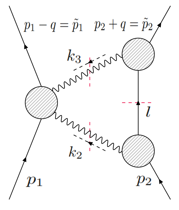
Figure 1: Triangle leading-singularity configuration Cachazo and Guevara (2020).

Having at hand the non-aligned HCL parametrization of the building blocks entering in (10), together with the HCL form of the optical parameter $\xi\rightarrow-\sigma^{2}v^{2}\frac{(1-y^{2})^{2}}{4y}$, it is now an easy task to compute the LS (10) using the Compton amplitude (1), since the problem has been reduced to a simple residue calculation. We organize the result of the residue evaluation as follows: Given the set of spin operators $\mathcal{H}=\{\mathcal{E}_{1},q{\cdot}s_{2},\sqrt{-q^{2}}p_{1}{\cdot}s_{2},\mathcal{E}_{2},q{\cdot}s_{1},\sqrt{-q^{2}}p_{2}{\cdot}s_{1}\}$, for the regular operators, and the spin operator basis $\mathcal{H}\to\tilde{\mathcal{H}}=\mathcal{H}\cup\{|q||s_{1}|,|q||s_{2}|\}$ for the exotic terms appearing starting at the fifth order in spin, we write the 2PM contribution of the triangle cut in the form

$$M_{\text{bare}}^{\text{2PM}}=\frac{\pi G^{2}}{\sqrt{-q^{2}}}\sum_{i,j}\Big{(}A_{i,j}\mathcal{H}^{\otimes^{i}}_{j}+B_{i,j}\tilde{\mathcal{H}}^{\otimes^{i}}_{j}\Big{)}\,.$$ (12)

Then, the main outputs from the LS evaluation are the $\{A_{i,j},B_{i,j}\}$ coefficients for a given spin structure in $\{\mathcal{H}^{\otimes^{i}}_{j},\tilde{\mathcal{H}}^{\otimes^{i}}_{j}\}$ respectively.

Up to the fourth order in spin, the LS construction easily recovers the triple cut coefficients reported in Bern et al. (2020); Kosmopoulos and Luna (2021); Chen et al. (2022) for SE Kerr BHs with generic spin orientations, upon evaluating to zero the contact deformations present at spin 4 in (1), as dictated by the Teukolsky solution (table 5). In this work, we extend the 2PM computation up to the sixth order in spin including both, regular and exotic contributions to (12). We provide LS results for generic coefficients parametrizing the Compton ansatz (1), which can then be specialized (if desired) to Teukolsky solutions (table 5) for the matching prescription described above.

Let us for brevity include here only the explicit results for the $s_{1}^{5}\times s_{2}^{0}$ sector of the 2PM triangle, leaving the results for the additional spin sectors, and up to the sixth order, for the ancillary files for this work anc . The spin structures for this sector are summarized in table 1, and the explicit coefficients for generic contact deformations are given in table 2. Additionally, we include in table 3 a dictionary that maps between our generic coefficient amplitude and the one reported in Bern et al. (2022c), hence providing a connection of the regular operators in (1) to the Lagrangian construction in Bern et al. (2022c).

Before moving to studding the content of these tables in more detail, and since most of the results of this work are included as ancillary files anc , let us here summarise the content of such files. We present three files named CoefficientsFile.wl, 2PMAmplitudeEikonalScatteringAngle.wl and CanonicalObservables.wl. The first of them contains the list of coefficients for the 1PM and 2PM amplitude as appearing in (12). In addition, the coefficients for the 1PM and 2PM eikonal phase for both CovSSC and CanSSC (see (9) and (13)) are included. Finally, replacement rules for the free coefficients of the Compton amplitude (1), as coming from Teukolsky, or the spin-shift-symmetry solutions (see table 5), and the dictionary included in table 3 are provided. The second file contains an explicit implementation of eqs. (12) and (13), as well as the explicit results for the aligned spin scattering angle (see below) in the CovSSC up to six order in spin. The remaining file, contains the results for 2PM canonical impulse and spin-kick (see (15)), up to sixth order in spin, including contributions from both, regular and exotic spin operators included in the Compton amplitude. Let us recall contributions from exotic operators appear only when at least one of the two spins is beyond the fourth order.

	$j$		$j$		$j$
$\frac{\mathcal{H}_{j}^{\otimes 5}}{\mathcal{E}_{1}}$	$1$	$\mathcal{E}_{1}^{4}$	$2$	$-q^{2}(p_{2}\cdot s_{1})^{2}\mathcal{E}_{1}^{2}$	$3$	$q^{4}(p_{2}\cdot s_{1})^{4}$
	$4$	$(q\cdot s_{1})^{2}\mathcal{E}_{1}^{2}$	$5$	$-q^{2}(q\cdot s_{1})^{2}(p_{2}\cdot s_{1})^{2}$	$6$	$(q\cdot s_{1})^{4}$
$\frac{\mathcal{\tilde{H}}_{j}^{\otimes 5}}{(p_{2}\cdot s_{1})\mathcal{E}_{1}|s_{1}|}$	$1$	$-q^{2}\mathcal{E}_{1}^{2}$	$2$	$q^{4}(p_{2}\cdot s_{1})^{2}$	$3$	$-q^{2}(q\cdot s_{1})^{2}$

Table 1: The independent spin structures for the $s_{1}^{5}\times s_{2}^{0}$ sector of the 2PM amplitude (12).

	$j$			$j$
$A_{5,j}$	$1$	$\frac{i\sigma\left(7-13\sigma^{2}\right)}{48\left(-1+\sigma^{2}\right)^{3}m_{1}^{7}m_{2}^{3}}-\frac{i\sigma\left(-96-60c_{2}^{(1)}+480c_{2}^{(2)}+135c_{3}^{(0)}+7\sigma^{4}\left(-4+120c_{2}^{(2)}+15c_{3}^{(0)}-15c_{3}^{(1)}\right)-90c_{3}^{(1)}+\sigma^{2}\left(304+60c_{2}^{(1)}-1320c_{2}^{(2)}-240c_{3}^{(0)}+195c_{3}^{(1)}\right)\right)}{1920\left(-1+\sigma^{2}\right)^{3}m_{1}^{8}m_{2}^{2}}$
	$2$	$\frac{i\sigma\left(-5+11\sigma^{2}\right)}{24\left(-1+\sigma^{2}\right)^{3}m_{1}^{5}m_{2}^{3}}-\frac{i\sigma\left(4\left(-36+75c_{2}^{(1)}+30c_{2}^{(2)}-\sigma^{2}\left(82+180c_{2}^{(1)}+240c_{2}^{(2)}-195c_{3}^{(0)}\right)+7\sigma^{4}\left(4+15c_{2}^{(1)}+30c_{2}^{(2)}-15c_{3}^{(0)}\right)-90c_{3}^{(0)}\right)+15\left(9-16\sigma^{2}+7\sigma^{4}\right)c_{3}^{(1)}\right)}{1920\left(-1+\sigma^{2}\right)^{3}m_{1}^{6}m_{2}^{2}}$
	$3$	$\frac{i\sigma\left(-1+3\sigma^{2}\right)}{48\left(-1+\sigma^{2}\right)^{3}m_{1}^{3}m_{2}^{3}}-\frac{i\sigma\left(3\left(-12+40c_{2}^{(1)}-40c_{2}^{(2)}-55c_{3}^{(0)}+25c_{3}^{(1)}\right)+\sigma^{2}\left(16+20\left(-13+7\sigma^{2}\right)c_{2}^{(1)}+120c_{2}^{(2)}+5\left(68-35\sigma^{2}\right)c_{3}^{(0)}+5\left(-29+14\sigma^{2}\right)c_{3}^{(1)}\right)\right)}{640\left(-1+\sigma^{2}\right)^{3}m_{1}^{4}m_{2}^{2}}$
	$4$	$-\frac{i\sigma\left(14\sigma^{2}\left(-4+120c_{2}^{(2)}+15c_{3}^{(0)}-15c_{3}^{(1)}\right)+3\left(16+20c_{2}^{(1)}-280c_{2}^{(2)}-60c_{3}^{(0)}+45c_{3}^{(1)}\right)\right)}{1920\left(-1+\sigma^{2}\right)m_{1}^{6}}$	$\frac{i\left(6c_{4}^{(0)}+7\left(-1+\sigma^{2}\right)c_{4}^{(1)}+2\left(4-7\sigma^{2}\right)c_{4}^{(2)}\right)}{64\left(-1+\sigma^{2}\right)m_{1}^{6}m_{2}}$	$1$	$B_{5,j}$
	$5$	$\frac{30i\sigma\left(4+12c_{2}^{(1)}-15c_{3}^{(0)}+6c_{3}^{(1)}\right)-7i\sigma^{3}\left(16+60c_{2}^{(1)}+120c_{2}^{(2)}-60c_{3}^{(0)}+15c_{3}^{(1)}\right)}{1920\left(-1+\sigma^{2}\right)m_{1}^{4}}$	$\frac{i\left(2\left(-4+7\sigma^{2}\right)c_{4}^{(0)}-7\left(-1+\sigma^{2}\right)c_{4}^{(1)}-6c_{4}^{(2)}\right)}{64\left(-1+\sigma^{2}\right)m_{1}^{4}m_{2}}$	$2$
	$6$	$-\frac{i\sigma\left(-3+7\sigma^{2}\right)m_{2}^{2}\left(-4+120c_{2}^{(2)}+15c_{3}^{(0)}-15c_{3}^{(1)}\right)}{1920m_{1}^{4}}$	$\frac{i\left(-1+7\sigma^{2}\right)m_{2}\left(c_{4}^{(1)}-2c_{4}^{(2)}\right)}{64m_{1}^{4}}$	$3$

Table 2: 2PM amplitude coefficients for the $s_{1}^{5}\times s_{2}^{0}$ sector of the two-body problem (12).

$$\boxed{\begin{split}c_{2}^{(2)}&\to\frac{374-165E_{1}+513E_{3}-33E_{4}-330E_{5}-495c_{3}^{(0)}+495c_{3}^{(1)}}{3960}\,,\\ c_{2}^{(1)}&\to\frac{153E_{3}-11\left(4+3E_{4}+15E_{5}\right)+2475c_{3}^{(0)}-990c_{3}^{(1)}}{1980}\,,\\ E_{7}&\to\frac{17}{30}+\frac{21E_{3}}{22}-\frac{E_{4}}{2}-\frac{E_{5}}{2}\,,\,\,E_{2}\to-E_{1}+\frac{3}{2}\left(E_{3}+E_{4}\right)\,,\,\,H_{3}\to\frac{3}{2}\,,\\ C_{i}&\to 1\,,i=2,3,4,5\,,\,\,H_{2}\to 1\,,\,\,E_{6}\to\frac{1}{6}\left(-2-3E_{3}\right)\,,\,\,H_{5}\to\frac{15E_{3}}{11}\,.\end{split}}$$

Table 3: Coefficient dictionary relating the regular terms of the $s_{1}^{5}\times s_{2}^{0}$ sector of the 2PM amplitude in this letter and the generic 2PM amplitude included in the ancillary files for ref. Bern et al. (2022c). The fixing $C_{i},H_{2}\to 1$ agrees with the minimal coupling matching of the 3-pt amplitude to the linearized Kerr metric, built in the Compton ansatz (1). Spin-shift symmetric solutions evaluated using the values of the last two columns of table 5 agree with those given in Bern et al. (2022c).

	$j$		$j$
$A_{5,j}$	$1$	$\frac{i\sigma\left(14m_{1}-2(13m_{1}+8m_{2})\sigma^{2}+7m_{2}\sigma^{4}\right)}{96m_{1}^{8}m_{2}^{3}(\sigma^{2}-1)^{3}}$	$4$	$\frac{7i\sigma^{3}}{48m_{1}^{6}(\sigma^{2}-1)}$
	$2$	$\frac{i\sigma\left(2m_{1}(11\sigma^{2}-5)+m_{2}(24-43\sigma^{2}+28\sigma^{4})\right)}{48m_{1}^{6}m_{2}^{3}(\sigma^{2}-1)^{3}}$	$5$	$\frac{7i\sigma(4\sigma^{2}-3)}{48m_{1}^{4}(\sigma^{2}-1)}$
	$3$	$\frac{i\sigma\left(m_{1}(6\sigma^{2}-2)+m_{2}(51-104\sigma^{2}+56\sigma^{4})\right)}{96m_{1}^{4}m_{2}^{3}(\sigma^{2}-1)^{3}}$	$6$	$\frac{im_{2}^{2}\sigma(7\sigma^{2}-3)}{96m_{1}^{4}}$
$B_{5,j}$	$1$	$\frac{i\eta(2+7\sigma^{2})}{24m_{1}^{6}m_{2}(\sigma^{2}-1)}$	$3$	$\frac{i\eta m_{2}(-1+7\sigma^{2})}{24m_{1}^{4}(\sigma^{2}-1)}$
	$2$	$\frac{i\eta(-5+14\sigma^{2})}{24m_{1}^{4}m_{2}(\sigma^{2}-1)}$

Table 4: 2PM LS coefficients for the $s_{1}^{5}\times s_{2}^{0}$ sector of the 2PM amplitude explicitly evaluated on the Teukolsky solutions table 5 for $\alpha=1$.

Spin-shift symmetry violation for Teukolsky solutions and the high-energy limit. It is illustrative to consider explicitly the 2PM LS coefficients evaluated on the Teukolsky solutions given in table 5; we include them in table 4. Inspection of these results reveals a breaking of the invariance of the amplitude under the transformation $a_{i}^{\mu}\to a_{i}^{\mu}+\varsigma_{i}q^{\mu}/q^{2}\,,$ with $\varsigma_{i}$ arbitrary constants, observed for the $a_{i}^{n\leq 4}$ cases Bern et al. (2022c); Aoude et al. (2022a, b). This happens not only due to the presence of the exotic operators but also because of the non-zero contributions of regular operators of the form $q\cdot s_{i}$ in table 1. One can also check shift-symmetric solutions for the Compton amplitude (table 5 ) induce a shift symmetric 2PM amplitude, as first observed in Aoude et al. (2022b).

Let us now comment on the high energy behavior of the 2PM amplitude for Teukolsky solutions (table 4). In the high energy limit ($\sigma\to\infty$), the 1PM amplitude scales as $\mathcal{O}(\sigma^{2})$ (here $\mathcal{E}_{i}\sim\sigma$). Having a well-defined 2PM amplitude in the high energy limit means it should grow no faster than the tree amplitude, as $\sigma\to\infty$ Bern et al. (2022c). This is however not the case for Teukolsky solutions of table 4. For instance, the term $A_{5,1}\mathcal{E}_{i}^{5}$ in (12) grows as $\sim\sigma^{4}$ as $\sigma\to\infty$, and analogously for the remaining contributions. This singular high-energy behavior propagates to the 2PM observables as we will discuss below in the context of the aligned spin scattering angle.

Eikonal phase and the aligned spin limit. The LS computation provides us with the ingredients needed to obtain the 2PM eikonal phase (8) for spinning objects satisfying both CovSSC and CanSSC, the latter obtained from the former by the shift of the impact parameter $\bm{b}\to\bm{b}+\sum_{i=1,2}\left(\frac{-\tau}{E_{i}+m_{i}}\right)\frac{\bm{p}\times\bm{s}_{i}}{m_{i}}$, a consequence of dressing the amplitude with the rotation factors (5). Results for the eikonal phase in the CanSSC will be needed when evaluating canonical observables via (15). We evaluate explicitly (8) and present the results for the eikonal phase in the CovSSC and in CoM coordinates in the ancillary files anc . The eikonal phase is organized schematically as

$$\chi_{\tau=0}^{(\text{2PM})}=\sum_{i,j}\frac{\pi G^{2}}{b^{2j+1}}\Big{(}L_{i,j}\,b\cdot\mathcal{S}^{j}+Ld_{i,j}\,b\cdot\tilde{\mathcal{S}}^{j}\Big{)}\,,$$ (13)

with $\{\mathcal{S}^{j},\tilde{\mathcal{S}}\}$ operators in the CoM version of $\{(\{b\}\cup\mathcal{H})^{\otimes j},(\{b\}\cup\tilde{\mathcal{H}})^{\otimes j}\}$ respectively, $b^{\mu}=(0,\bm{b},0)$, and the coefficients $\{L_{i,j},Ld_{i,j}\}$ are functions of $m_{i},E_{i},\sigma$, and linear combinations of the amplitude coefficients $\{A_{i,j},B_{i,j}\}$ respectively. From this, we then specialize the eikonal phase to the case in which the rotating objects have their spins aligned in the direction of the angular momentum of the system, $\bm{b}\cdot\bm{s}_{i}=\bm{p}\cdot\bm{s}_{i}=0$ (see $e.g.$ Kosmopoulos and Luna (2021)) and compute the 2PM aligned spin scattering angle via $\frac{\partial\chi_{\tau=0}}{\partial|b|}$. In this limit, the exotic operators do not contribute to the scattering angle as observed in Bautista et al. (2022), therefore for Teukolsky solutions, the angle itself is independent of the analytic continuation procedure used to match (1) to the GW scattering process. Results up to the sixth order in spin for the contributing regular operators are included in the ancillary files for generic contact deformations in (1) anc .

Let us now comment on the comparison of the aligned spin scattering angle results in this work to the ones presented in Guevara et al. (2019); Bautista et al. (2022) for generic, spin-shift-symmetric Bern et al. (2022c); Aoude et al. (2022a, b), and Teukolsky Compton coefficients Bautista et al. (2022). The HCL prescription of Guevara et al. (2019) to compute the aligned spin scattering angle by fixing $\beta=1$, in turn hiddenly sets $q{\cdot}s_{j}\to i\frac{\mathcal{E}_{j}}{m_{1}m_{2}\sigma v}$ as well as $|q|\to 0\Rightarrow|q|p_{i}{\cdot}s_{j}\to 0$ in (11), as can be seen from the last line of (23). The latter replacement does not have any problem since in the aligned spin limit the equality $\bm{p}{\cdot}\bm{s}_{i}=0$ is satisfied. Similarly, the former identification does not possess any subtleties for combinations of spin operators of the form $(k_{2}-k_{3}){\cdot}s_{i}$, since these combinations themselves are independent of $q^{\mu}$, as can be checked by direct inspection of eq. (11). However, for spin operators where $k_{i}{\cdot}s_{i}$ have individual appearances – as is the case for some of the contact deformations in (1) – the identification $q.s_{j}\to i\frac{\mathcal{E}_{j}}{m_{1}m_{2}\sigma v}$ discards $\mathcal{O}(q^{2})$ terms (see (23)) that are important for the aligned spin angle. For quadratic terms, for instance, this map is equivalent to setting $(q{\cdot}s_{i})^{2}\to(q{\cdot}s_{i})^{2}-q^{2}s_{i}^{2}\,,$ which in two-dimensional impact parameter space implies $3(\bm{b}{\cdot}\bm{s}_{i})^{2}-\bm{b}^{2}\bm{s}_{\perp i}^{2}\to 3(\bm{b}{\cdot}\bm{s}_{i})^{2}-2\bm{b}^{2}\bm{s}_{\perp i}^{2}\,,$ – with $\bm{s}_{\perp i}$ the components of the spin along $\bm{b}$ – therefore removing some terms that survive in the aligned spin limit ($\bm{b}{\cdot}\bm{s}_{i}=0$). An analogous analysis follows for higher spin contributions. Interestingly, this identification removes the terms in the amplitude that did not have a well-defined high energy limit. The spin-shift symmetric result of Bern et al. (2020); Aoude et al. (2022b) has also a well-defined high-energy limit. Finally, let us note the angle for the lower spin cases Guevara et al. (2019) did not face this ambiguity since only the combination $(2w-k_{2}-k_{3})\cdot a_{i}$ – independent of $q{\cdot}a_{i}$ terms – appeared in the Compton amplitude.

Keeping all the contributions to the scattering angle, and continuing with the theme of the spin 5 sector for briefness, the aligned spin angle takes the form

$$\begin{split}\theta^{(5)}=&\,\theta^{(5)}_{\text{BGKV}}-\frac{9\pi EG^{2}}{256\,b^{7}\,v(1-v^{2})}\Big{[}(a_{1}^{5}m_{2}{+}a_{2}^{5}m_{1})K_{1}\\ &\hskip 71.13188pt+(a_{1}^{3}m_{2}{+}a_{2}^{3}m_{1})a_{1}a_{2}\,K_{2}\Big{]}\,,\end{split}$$ (14)

where $K_{1}=80(1-v^{2})c_{2}^{(1)}+40(8+13v^{2})c_{2}^{(2)}+(4-11v^{2})(4-15c_{3}^{(0)})-105v^{2}c_{3}^{(1)}$ and $K_{2}=-40\big{[}2(1-v^{2})c_{1}^{(1)}+(8+13v^{2})c_{1}^{(2)}\big{]}$, and with $\theta^{(5)}_{\text{BGKV}}$ the scattering angle reported in the arXiv v2 of Bautista et al. (2022). Teukolsky solutions (table 5) give $K_{1}|_{\text{Teuk.}}=20(12-5v^{2})$ and $K_{2}|_{\text{Teuk.}}=0$, therefore resulting into a scattering angle divergent as $v\to 1$ as expected from the discussion above. Let us stress this result is independent of the analytic continuation procedure for the matching of eq. 1 to the Teukolsky solutions. Finally, for a shift-symmetric amplitude (see the last two columns of table 5), $K_{1}=K_{2}=0$ recovers the result of Bern et al. (2022c); Aoude et al. (2022b), and the angle is well behaved in the high-energy limit. The sixth order in spin angle can be obtained analogously, explicit results can be found in the ancillary files anc . Up to $\mathcal{O}(a^{6})$, and in the probe limit, our results are in complete agreement with the ones reported in Damgaard et al. (2022); contact deformations of the Compton amplitude do not contribute to the 2PM angle in this case. In addition, only the next order in the symmetric mass ratio is needed to fully obtain our 2PM results, as expected from the spin version of the mass polynomiality rule Damour (2020).

2PM canonical observables. We are finally in ready to compute the conservative 2PM canonical observables for $2\to 2$ scattering of SE Kerr BHs. For this, we will follow the prescription provided by the authors of Bern et al. (2020); Kosmopoulos and Luna (2021). It was noticed in these references that the conservative observables $\Delta\mathcal{O}\in\{\Delta\bm{p}_{\perp},\Delta\bm{s}_{a}\}$ at 2PM can be obtained from the eikonal phase in the CanSSC $\chi\equiv\chi_{\tau=1}=\chi^{\text{1PM}}_{\tau=1}+\chi^{\text{2PM}}_{\tau=1}+\cdots$, via

$$\begin{split}\Delta\mathcal{O}=&-\{\mathcal{O},\chi\}-\frac{1}{2}\{\chi,\{\mathcal{O},\chi\}\}-\mathcal{D}_{SL}(\chi,\{\mathcal{O},\chi\})\\ &+\frac{1}{2}\{\mathcal{O},\mathcal{D}_{SL}(\chi,\chi)\}\,,\end{split}$$ (15)

with the Poisson bracket given by

$$\{f,g\}{=}\frac{\partial f}{\partial p_{\perp}^{j}}\frac{\partial g}{\partial b^{j}}{-}\frac{\partial g}{\partial p_{\perp}^{j}}\frac{\partial f}{\partial b^{j}}{+}\sum_{a=1,2}\epsilon^{ijk}\frac{\partial f}{\partial s^{i}_{a}}\frac{\partial g}{\partial s^{j}_{a}}s_{a,k}\,,$$ (16)

and the spin derivative operator

$$\mathcal{D}_{SL}(f,g){=}\frac{1}{\bm{p}^{2}}\sum_{a,1,2}\left(\frac{\partial f}{\partial s_{a}^{j}}\frac{\partial g}{\partial b^{j}}\bm{s}_{a}{\cdot}\bm{p}{-}p^{j}\frac{\partial f}{\partial s_{a}^{j}}\bm{s}_{a}{\cdot}\nabla_{\bm{b}}g\right)$$ (17)

Using this prescription, and the results for the 1 and 2PM eikonal phase derived above, we have computed the 2PM observables up to the six order in spin for generic contact deformations in eq. 1, which can then specialize to Teukolsky solutions. The expressions are however too long to be included in this letter and we, therefore, provide them in the ancillary material for this work anc . We include results for the transverse impulse and individual spin kicks in the CanSSC up to the sixth order in spin for both regular and exotic contributions to the 2PM amplitude in the CoM frame. Up to the fourth order in spin our results completely agree with those reported in Bern et al. (2020); Kosmopoulos and Luna (2021); Chen et al. (2022) upon setting to zero the contact deformations at this order, and after the authors of Chen et al. (2022) fixed some of the reported observables that had an initial disagreement with the ones presented in this work.

Conclusions. In this work, we have computed the canonical observables for the conservative SE Kerr two-body problem at second order in the PM expansion and up to sixth order in spin, for generic spin orientation. The results in this work are presented for generic Compton contact deformations, which can be specialized to Teukolsky solutions. In the latter case, the 2PM amplitude breaks the conjecture spin-shift symmetry for Kerr BHs Bern et al. (2022c); Aoude et al. (2022a, b), however producing observables with a non-smooth high energy behavior. This leaves as an open problem understanding if the unhealthy high-energy behavior is a consequence of the analytic continuation to the SE Kerr region and observables for actual Kerr solutions ($a^{\star}\leq 1$) feature a well-defined high energy limit , perhaps guiding possible realizations of the spin-shift symmetry in this scenario. For the generic coefficient case, we have presented a dictionary that maps the Compton operators in this letter to the Lagrangian and Hamiltonian constructions in Bern et al. (2022c). Finally, the identification of regular and exotic contributions with true conservative and absorptive contributions in the Kerr binary problem is a subject that requires further scrutiny and we leave for future work.

Acknowledgments. We would like to thank Rafael Aoude, Stefano De Angelis, Leonardo de la Cruz, Alfredo Guevara, Kays Haddad, Carlo Heissenberg, Andreas Helset, Chris Kavanagh, Dimitrios Kosmopoulos, David Kosower, Andres Luna and M. V. S. Saketh for useful discussion. We are also grateful to Jung-Wook Kim and Ming-Zhi Chung for the continuum discussion and for sharing an updated version of their 2PM observables Chen et al. (2022) up to spin 4. We would like to especially thank Justin Vines for sharing his unpublished notes on the generalization of the HCL for non-aligned spins, and Leonardo de la Cruz for his comments on the manuscript. This work has been supported by the European Research Council under Advanced Investigator Grant ERC–AdG–885414.

Appendix A Appendix A: Triangle Leading singularity and the holomorphic classical limit for generic spin orientation

In this appendix, we present an extension of the Holomorphic Classical Limit (HCL) Guevara (2019) and the triangle Leading Singularity (LS) Cachazo and Guevara (2020) constructions for spinning particles for generic spin directions. This is based on an unpublished note by Justin Vines to whom we are grateful.

We start by constructing a suitable local 4-dimensional reference frame all’a Penrose, Rindler, and Chandrasekhar Penrose and Rindler (1984) as follows: Given a two-dimensional basis of massless spinors $\mathcal{L}=\{|\chi\rangle,|\psi\rangle\}$, together with the co-basis $\tilde{\mathcal{L}}=\{[\chi|,[\psi|\}$, and whose elements satisfy the normalization conditions $\langle\chi\psi\rangle=[\chi\psi]=\frac{1}{\sqrt{2}},$ we can adapt the spinor bases to the vector tetrad $\{e^{\mu}_{(a)}\}=\{\mathfrak{t}^{\mu},\mathfrak{x}^{\mu},\mathfrak{y}^{\mu},\mathfrak{z}^{\mu}\}$, with $\mathfrak{t}^{2}=-1$ and $\mathfrak{x}^{2}=\mathfrak{y}^{2}=\mathfrak{z}^{2}=-1$, via the usual vector-spinors map $V^{\alpha\dot{\alpha}}=(\sigma^{\mu})^{\alpha\dot{\alpha}}v_{\mu}$, as follows:

$$\begin{split}\mathfrak{T}^{\alpha\dot{\alpha}}&=(\sigma^{\mu})^{\alpha\dot{\alpha}}\mathfrak{t}_{\mu}=\sqrt{2}(|\chi\rangle[\psi|+|\psi\rangle[\chi|)\,,\\ \mathfrak{Z}^{\alpha\dot{\alpha}}&=(\sigma^{\mu})^{\alpha\dot{\alpha}}\mathfrak{z}_{\mu}=\sqrt{2}(|\chi\rangle[\psi|-|\psi\rangle[\chi|)\,,\\ \mathfrak{X}^{\alpha\dot{\alpha}}&=(\sigma^{\mu})^{\alpha\dot{\alpha}}\mathfrak{x}_{\mu}=\sqrt{2}(|\chi\rangle[\chi|+|\psi\rangle[\psi|)\,,\\ \mathfrak{Y}^{\alpha\dot{\alpha}}&=(\sigma^{\mu})^{\alpha\dot{\alpha}}\mathfrak{y}_{\mu}=i\sqrt{2}(|\chi\rangle[\chi|-|\psi\rangle[\psi|)\,.\end{split}$$ (18)

Here $\sigma^{\mu}$ are the Pauli matrices and shall not be confused with the Lorentz boost factor $\sigma$ which is a scalar.

This tetrad spans the 4-dimensional flat spacetime and therefore any vector (including the spin) can be constructed from a linear combination of vectors in $\{e^{\mu}_{(a)}\}$. Notice in general the spinors in $\mathcal{L}$ are not related to those in $\tilde{\mathcal{L}}$ by complex conjugation and therefore the tetrad decomposition admits vectors with complex values. Thus, a generic vector $q^{\mu}$ will be given by the decomposition

$$Q^{\alpha\dot{\alpha}}=(\sigma^{\mu})^{\alpha\dot{\alpha}}q_{\mu}=a_{q}|\chi\rangle[\chi|+b_{q}|\chi\rangle[\psi|+c_{q}|\psi\rangle[\chi|+d_{q}|\psi\rangle[\psi|\,,$$ (19)

where $a_{q}=\frac{1}{2}\langle\psi|Q|\psi]$, and analogously for the other components. Lorentz invariant products are obtained in the usual form

$$q^{2} =\frac{1}{2}\text{tr}(Q\cdot\bar{Q})=\frac{1}{2}(c_{q}b_{q}-a_{q}d_{q})\,,\,\,\,\,p{\cdot}q=\frac{1}{2}\text{tr}(Q\cdot\bar{P})=\frac{1}{4}(b_{q}c_{p}+b_{p}c_{q}-a_{q}d_{p}-a_{p}d_{q})\,.$$ (20)

2PM Triangle kinematics: The next task is to use this reference frame to parametrize the momenta of the particles in the triangle cut fig. 1. Unlike for the aligned spin scenario, here we will take the momentum transfer $q=k_{2}+k_{3}$ so that $q^{2}=2k_{2}{\cdot}k_{3}\neq 0$. We orient the tetrad $\{e_{(a)}^{\mu}\}$ in such a way that the BH 2 is at rest, the BH 1 moves in the $\mathfrak{z}$-direction with relative velocity $v$, and the component of $q^{\mu}$ orthogonal to $p_{1}^{\mu}$ and $p_{2}^{\mu}$ lies in the $\mathfrak{x}$-direction. It follows then

$$p_{1}^{\mu}=m_{1}\sigma(\mathfrak{t}^{\mu}+v\mathfrak{z}^{\mu})\,,\,\,\,p_{2}^{\mu}=m_{2}\mathfrak{t}^{\mu}\,,\,\,\,q{\cdot}\mathfrak{y}=0\,.$$ (21)

The momentum transfer $q^{\mu}$ can be parametrized using the decomposition (19). With help of the on-shell conditions $p_{1}{\cdot}q=q^{2}/2,\,\,p_{2}{\cdot}q=-q^{2}/2$ and $q{\cdot}\mathfrak{y}=0$, and solving for the coefficients $a_{q},b_{q},c_{q},d_{2}$ in terms of the kinematic variables $m_{1},m_{2},\sigma,|q|$, where $|q|=\sqrt{-q^{2}}$, one explicitly gets

$$b_{q}=\frac{m_{2}+m_{1}(1+v)\sigma}{\sqrt{2}m_{1}m_{2}\sigma v}|q|^{2}\,,\,\,\,c_{q}=-\frac{m_{2}+m_{1}(1-v)\sigma}{\sqrt{2}m_{1}m_{2}\sigma v}|q|^{2}\,,\,\,d_{q}=a_{q}=\pm\sqrt{b_{q}^{2}c_{q}^{2}+2|q|^{2}}\,.$$ (22)

HCL parametrization: The final task is to find a suitable parametrization for the internal massless momenta in such a way the classical limit of the triangle diagram fig. 1 is easily obtained. For that, let us introduce the new spinor bases $\{|\hat{\lambda}\rangle,|\hat{\eta}\rangle\}$ and $\{[\hat{\lambda}|,[\hat{\eta}|\}$ for the first massive line, together with $\{|\lambda\rangle,|\eta\rangle\}$ and $\{[\lambda|,[\eta|\}$ for the second massive line, following Guevara Guevara (2019). In these new bases, the external momenta are parametrized as

$$\begin{split}P_{1}&=|\hat{\eta}]\bra{\hat{\lambda}}+|\hat{\lambda}]\bra{\hat{\eta}}\,,\,\,\,\,\tilde{P}_{1}=\beta^{\prime}|\hat{\eta}]\bra{\hat{\lambda}}+\frac{1}{\beta^{\prime}}|\hat{\lambda}]\bra{\hat{\eta}}+|\hat{\lambda}]\bra{\hat{\lambda}},\\ P_{2}&=|\eta]\bra{\lambda}+|\lambda]\bra{\eta}\,,\,\,\,\,\tilde{P}_{2}=\beta|\eta]\bra{\lambda}+\frac{1}{\beta}|\lambda]\bra{\eta}+|\lambda]\bra{\lambda},\\ Q&=P_{1}-\tilde{P}_{1}=-P_{2}+\tilde{P}_{2}\,,\,\,\,\,\Rightarrow\,\,|q|^{2}=m_{2}^{2}\frac{(\beta-1)^{2}}{\beta}\,,\end{split}$$ (23)

where $Q$ is the complex momentum transfer matrix. Thus, as $|q|\to 0$ (as $\beta\to 1$) one recovers the usual HCL result $Q\to|\lambda]\langle\lambda|$, but now we keep subleading terms in $(\beta-1)$. The on-shell conditions $P_{1}^{2}=\tilde{P}_{1}^{2}=m_{1}^{2}$ and $P_{2}^{2}=\tilde{P}_{2}^{2}=m_{2}^{2}$, impose the normalization for the spinors $\braket{\hat{\lambda}\hat{\eta}}=[\hat{\lambda}\hat{\eta}]=m_{1}$ and $\braket{\lambda\eta}=[\lambda\eta]=m_{2}$. For the internal gravitons, the spinor helicity variables are analogously parametrized via

$$\begin{split}\ket{k_{2}}&=\frac{1}{\beta+1}\left(\left(\beta^{2}-1\right)\ket{\eta}-\frac{1+\beta y}{y}\ket{\lambda}\right),\,\,\,|k_{2}]=\frac{1}{\beta+1}\left(\left(\beta^{2}-1\right)y|\eta]+(1+\beta y)|\lambda]\right),\\ \ket{k_{3}}&=\frac{1}{\beta+1}\left(\frac{\beta^{2}-1}{\beta}\ket{\eta}+\frac{1-y}{y}\ket{\lambda}\right),\,\,\,|k_{3}]=\frac{1}{\beta+1}\left(-\beta\left(\beta^{2}-1\right)y|\eta]+(1-\beta^{2}y)|\lambda]\right).\end{split}$$ (24)

Here $y$ is the loop integration parameter entering in (10). Imposing consistency between the HCL (23) and the tetrad (19) (21) parametrizations, allows us to solve for $\{|\lambda\rangle,|\eta\rangle,[\lambda|,[\eta|\}$ in terms of $\{|\chi\rangle,|\psi\rangle,[\chi|,[\psi|\}$, up to an irrelevant little group scale $\bar{\omega}$ that cancels from the final result. Using, $\beta=1+\frac{|q|}{2m_{2}^{2}}(|q|\mp\sqrt{|q|^{2}+4m_{2}^{2}})$, as well as the solutions (22) for the on-shell conditions for the external momenta, to leading order in $|q|$, we find

$$\begin{split}|\lambda\rangle&=\bar{\omega}\sqrt{|q|}(|\chi\rangle+|\psi\rangle)+\mathcal{O}(q^{3/2})\,,\,\,\,\,[\lambda|=\frac{\sqrt{2}|q|}{\bar{\omega}}([\chi|-[\psi|)+\mathcal{O}(q^{3/2})\,,\\ |\eta\rangle&=-\frac{m_{2}\bar{\omega}}{\sqrt{|q|}}|\chi\rangle+\mathcal{O}(q^{1/2})\,,\,\,\,\,[\eta|=\frac{m_{2}}{\sqrt{|q|\bar{\omega}}}[\chi|+\mathcal{O}(q^{1/2})\,.\end{split}$$ (25)

These solutions can be replaced into (24) to obtain analog expressions for the internal graviton variables. Explicitly, in the tetrad basis, to leading order in $|q|$, the internal graviton momenta take the form

$$\begin{split}k_{2}^{\mu}&=\frac{|q|}{2\sigma v}\big{[}\sqrt{z^{2}-1}(u^{\mu}-\sigma\mathfrak{t}^{\mu})+\sigma v(\mathfrak{x}^{\mu}+iz\mathfrak{y}^{\mu})\big{]}\,,\\ k_{3}^{\mu}&=-\frac{|q|}{2\sigma v}\big{[}\sqrt{z^{2}-1}(u^{\mu}-\sigma\mathfrak{t}^{\mu})-\sigma v(\mathfrak{x}^{\mu}-iz\mathfrak{y}^{\mu})\big{]}\,,\\ w^{\mu}&=-\frac{|q|}{2\sigma(1-vz)}\Big{[}(u^{\mu}-\sigma\mathfrak{t}^{\mu})z+\sigma v(\sqrt{z^{2}-1}\mathfrak{t}^{\mu}+i(z^{2}-1)\mathfrak{y}^{\mu})\Big{]}\,,\end{split}$$ (26)

where the incoming 4-velocity $u^{\mu}=p_{1}^{\mu}/m_{1}$. Here we have used (3) as a definition for $w^{\mu}$, and the gauge (3), together with the Lorentz products $p_{1}{\cdot}k_{2}=-\frac{1}{2}m_{1}|q|\sigma v\sqrt{z^{2}-1}$ and $p_{1}{\cdot}\epsilon_{2}=-\frac{1}{2[23]}m_{1}|q|\sigma(1+vz)$ entering in (3). We can further identify the momentum transfer $q^{\mu}=|q|\mathfrak{x}^{\mu}$, whereas $\mathfrak{y}^{\alpha}=\varepsilon^{\delta\alpha\beta\gamma}\mathfrak{t}_{\delta}\mathfrak{x}_{\beta}\mathfrak{z}_{\gamma}$, since $\varepsilon_{\alpha\beta\gamma\delta}\mathfrak{t}^{\alpha}\mathfrak{x}^{\beta}\mathfrak{y}^{\gamma}\mathfrak{z}^{\delta}=1$, with $\varepsilon^{\alpha\beta\gamma\delta}$ the four-dimensional Levi-Civita symbol. In terms of the external momenta (21), and with $\mathfrak{y}^{\alpha}=\frac{1}{m_{1}m_{2}\sigma v|q|}\mathcal{E}^{\alpha}$, where $\mathcal{E}^{\alpha}$ was defined bellow (11), the massless momenta (26) recover the main text expressions (11).

Appendix B Appendix B: Compton Amplitude from Teukolsky solutions

The explicit form of the amplitude (1), contains the function of contact deformations $P_{\xi}$ Bautista et al. (2022):

$$P_{\xi}= \sum_{m=0}^{2}\xi^{m-1}(w\cdot a)^{4-2m}(w\cdot a-k_{2}\cdot a)^{m}(w\cdot a+k_{3}\cdot a)^{m}r^{(m)}_{|a|}(k_{2}\cdot a,-k_{3}\cdot a,w\cdot a)$$

$$+\sum_{m=0}^{\infty}\left[\frac{(w\cdot a)^{2m+6}}{\xi^{m+2}}p^{(m)}_{|a|}(k_{2}\cdot a,-k_{3}\cdot a,w\cdot a)\right.$$

$$\left.+\xi^{m+2}(w\cdot a-k_{2}\cdot a)^{m+3}(w\cdot a+k_{3}\cdot a)^{m+3}\,q^{(m)}_{|a|}(k_{2}\cdot a,-k_{3}\cdot a,w\cdot a)\right]\,,$$ (27)

where the multivariable polynomials $p^{(m)}_{|a|},q^{(m)}_{|a|},r^{(m)}_{|a|}$ up to order $a^{6}$ have the explicit form:

$$\begin{split}r_{|a|}^{(m)}&=c_{1}^{(m)}+c_{2}^{(m)}(k_{2}{\cdot}a-k_{3}{\cdot}a)+c_{3}^{(m)}w{\cdot}a+c_{4}^{(m)}|a|\omega\\ &\quad+c_{5}^{(m)}(w{\cdot}a-k_{2}{\cdot}a)(w{\cdot}a+k_{3}{\cdot}a)\\ &\quad+c_{6}^{(m)}(2w{\cdot}a-k_{2}{\cdot}a+k_{3}{\cdot}a)w{\cdot}a\\ &\quad+c_{7}^{(m)}(2w{\cdot}a-k_{2}{\cdot}a+k_{3}{\cdot}a)^{2}+c_{8}^{(m)}(w{\cdot}a)^{2}\\ &\quad+c_{9}^{(m)}(k_{2}{\cdot}a-k_{3}{\cdot}a)|a|\omega+c_{10}^{(m)}w{\cdot}a|a|\omega+\mathcal{O}(a^{3})\end{split}$$ (28)

$$p_{|a|}^{(m)}=d_{1}^{(m)}+\mathcal{O}(a)\,,\qquad q_{|a|}^{(m)}=f_{1}^{(m)}+\mathcal{O}(a)\,.$$ (29)

Here $c_{i}^{m},d_{i}^{(m)}$ and $f_{i}^{(m)}$ are free coefficients that can be fixed either by imposing spin-shift symmetry arguments, or by matching the explicit BHPT computation. The different choices with their respective explicit values are indicated in table 5.

Spin	Spurious-pole	Free Coeffs.	Teukolsky Solutions		Spin-Shift-Sym.	Free Coeffs.
$a^{4}$		$c_{1}^{(i)},\,\,i=0,1,2$	$c_{1}^{(i)}=0,\,\,i=0,1,2$		$\begin{aligned} c_{1}^{(i)}&=0,\,i=1,2\end{aligned}$	$c_{1}^{(0)}$
$a^{5}$	$c_{3}^{(2)}=4/15-c_{3}^{(0)}+c_{3}^{(1)}$	$\begin{aligned} c_{2}^{(i)}&,\,\,i=0,1,2\\ c_{3}^{(i)}&,\,\,i=0,1\\ c_{4}^{(i)}&,\,\,i=0,1,2\end{aligned}$	$\begin{aligned} c_{2}^{(i)}&=0,\,\,i=0,1,2\\ c_{3}^{(0)}&=\alpha\frac{64}{15}\,,\,c_{3}^{(1)}=\alpha\frac{16}{3}\,,\\ c_{3}^{(2)}&=\frac{4}{15}(1+4\alpha)\,,\\ c_{4}^{(0)}&=\eta\alpha\frac{64}{15}\,,\\ c_{4}^{(1)}&=\eta\alpha\frac{16}{5}\,,\,c_{4}^{(2)}=\eta\frac{4}{15}\end{aligned}$		$\begin{aligned} c_{j}^{(i)}&=0,\,\,i=1,2,\,\,j=2,3\\ c_{3}^{(0)}&=\frac{4}{15},\,\,c_{4}^{(i)}=0\,,i=0,1,2\end{aligned}$	$c_{2}^{(0)}$
$a^{6}$	$\begin{aligned} c_{10}^{(2)}&=c_{10}^{(1)}-c_{10}^{(0)}\\ d_{1}^{(0)}=&-\frac{8}{45}+4\sum_{i=0}^{2}(-1)^{i}c_{7}^{(i)}\\ &+\sum_{j=5}^{6}\sum_{i=0}^{2}(-1)^{i}c_{j}^{(i)}\\ f_{1}^{(0)}=&\frac{4}{45}\\ &+\sum_{i=0}^{2}\sum_{j\in\{6,8\}}(-1)^{i}c_{j}^{(i)}\end{aligned}$	$\begin{aligned} c_{5}^{(i)}&,\,\,i=0,1,2\\ c_{6}^{(i)}&,\,\,i=0,1,3\\ c_{7}^{(i)}&,\,\,i=0,1,2\\ c_{8}^{(i)}&,\,\,i=0,1,3\\ c_{9}^{(i)}&,\,\,i=0,1,2\\ c_{10}^{i}&,\,\,i=0,1\end{aligned}$	$\begin{aligned} c_{j}^{(i)}&=0,\,\,i=0,1,2,\,\,j=5,7\\ c_{6}^{(0)}&=\alpha\frac{128}{45}\,,\,c_{6}^{(1)}=\alpha\frac{32}{9}\,,\\ c_{6}^{(2)}&=\frac{8}{45}(1{+}4\alpha)\,,c_{8}^{(0)}={-}\alpha\frac{512}{45},\,\\ c_{8}^{(1)}&={-}\alpha\frac{160}{9},\,c_{8}^{(2)}={-}\frac{16}{45}(1{+}19\alpha),\\ c_{9}^{(0)}&=-\eta\alpha\frac{128}{45}\,,\,c_{9}^{(1)}=-\eta\alpha\frac{32}{15}\,,\\ c_{9}^{(2)}&=-\eta\frac{8}{45},\\ c_{10}^{(0)}&=-\eta\alpha\frac{256}{45},\\ c_{10}^{(1)}&=-\eta\alpha\frac{352}{45},c_{10}^{(2)}=-\eta\alpha\frac{32}{15}\\ d_{1}^{(0)}&=0\,,\,f_{1}^{(0)}=-\frac{4}{45}(1+4\alpha)\end{aligned}$		$\begin{aligned} c_{j}^{(i)}&=0,\,\,i=0,1,2,\,\,j=5,9,10\\ c_{j}^{(i)}&=0,\,\,i=1,2,\,\,j=6,7,8\\ c_{8}^{(0)}&=-\frac{4}{45}-c_{6}^{(0)}\\ f_{1}^{(0)}&=0\\ d_{1}^{(0)}&=-\frac{8}{45}+c_{6}^{(0)}+4c_{7}^{(0)}\end{aligned}$	$c_{6}^{(0)},c_{7}^{(0)}$

Table 5: Second column:. Spurious pole cancellation constraints on the Compton ansatz. Third column: Free contact coefficients after imposing the constraint of the second column. Fourth column: Match to low-energy Teukolsky solutions. Here $\alpha=1$, is a coefficient tracking non-rational (digamma functions) contributions, and $\eta=0,\pm 1$, is a parameter that keeps track of the regular ($\eta=0$), and exotic ($\eta=\pm 1$) pieces of the scattering amplitude. Fifth column: Spin-shift symmetry constraints on the Compton ansatz. Sixth column: Free parameters for a spin-shift symmetric Compton ansatz. Table recreated from Bautista et al. (2022).

References

- Cheung et al. (2018) C. Cheung, I. Z. Rothstein, and M. P. Solon, Phys. Rev. Lett. 121, 251101 (2018), arXiv:1808.02489 [hep-th] .
- Kosower et al. (2019) D. A. Kosower, B. Maybee, and D. O’Connell, JHEP 02, 137 (2019), arXiv:1811.10950 [hep-th] .
- Bern et al. (2022a) Z. Bern, J. Parra-Martinez, R. Roiban, M. S. Ruf, C.-H. Shen, M. P. Solon, and M. Zeng, PoS LL2022, 051 (2022a).
- Bern et al. (2022b) Z. Bern, J. Parra-Martinez, R. Roiban, M. S. Ruf, C.-H. Shen, M. P. Solon, and M. Zeng, Phys. Rev. Lett. 128, 161103 (2022b), arXiv:2112.10750 [hep-th] .
- Bern et al. (2021) Z. Bern, J. Parra-Martinez, R. Roiban, M. S. Ruf, C.-H. Shen, M. P. Solon, and M. Zeng, Phys. Rev. Lett. 126, 171601 (2021), arXiv:2101.07254 [hep-th] .
- Bern et al. (2020) Z. Bern, A. Luna, R. Roiban, C.-H. Shen, and M. Zeng, (2020), arXiv:2005.03071 [hep-th] .
- Bern et al. (2019) Z. Bern, C. Cheung, R. Roiban, C.-H. Shen, M. P. Solon, and M. Zeng, Phys. Rev. Lett. 122, 201603 (2019), arXiv:1901.04424 [hep-th] .
- Dlapa et al. (2023) C. Dlapa, G. Kälin, Z. Liu, J. Neef, and R. A. Porto, Phys. Rev. Lett. 130, 101401 (2023), arXiv:2210.05541 [hep-th] .
- Dlapa et al. (2022) C. Dlapa, G. Kälin, Z. Liu, and R. A. Porto, Phys. Lett. B 831, 137203 (2022), arXiv:2106.08276 [hep-th] .
- Kälin et al. (2020) G. Kälin, Z. Liu, and R. A. Porto, Phys. Rev. Lett. 125, 261103 (2020), arXiv:2007.04977 [hep-th] .
- Mogull et al. (2021) G. Mogull, J. Plefka, and J. Steinhoff, JHEP 02, 048 (2021), arXiv:2010.02865 [hep-th] .
- Jakobsen et al. (2022a) G. U. Jakobsen, G. Mogull, J. Plefka, and B. Sauer, (2022a), arXiv:2207.00569 [hep-th] .
- Elkhidir et al. (2023) A. Elkhidir, D. O’Connell, M. Sergola, and I. A. Vazquez-Holm, (2023), arXiv:2303.06211 [hep-th] .
- Brandhuber et al. (2023) A. Brandhuber, G. R. Brown, G. Chen, S. De Angelis, J. Gowdy, and G. Travaglini, (2023), arXiv:2303.06111 [hep-th] .
- Herderschee et al. (2023) A. Herderschee, R. Roiban, and F. Teng, (2023), arXiv:2303.06112 [hep-th] .
- Georgoudis et al. (2023) A. Georgoudis, C. Heissenberg, and I. Vazquez-Holm, (2023), arXiv:2303.07006 [hep-th] .
- Di Vecchia et al. (2021) P. Di Vecchia, C. Heissenberg, R. Russo, and G. Veneziano, (2021), arXiv:2104.03256 [hep-th] .
- Abbott et al. (2016) B. P. Abbott et al. (LIGO Scientific, Virgo), Phys. Rev. Lett. 116, 061102 (2016), arXiv:1602.03837 [gr-qc] .
- Levi and Steinhoff (2015) M. Levi and J. Steinhoff, JHEP 09, 219 (2015), arXiv:1501.04956 [gr-qc] .
- Bern et al. (2022c) Z. Bern, D. Kosmopoulos, A. Luna, R. Roiban, and F. Teng, (2022c), arXiv:2203.06202 [hep-th] .
- Chung et al. (2020a) M.-Z. Chung, Y.-t. Huang, J.-W. Kim, and S. Lee, JHEP 05, 105 (2020a), arXiv:2003.06600 [hep-th] .
- Jakobsen and Mogull (2022a) G. U. Jakobsen and G. Mogull, Phys. Rev. Lett. 128, 141102 (2022a), arXiv:2201.07778 [hep-th] .
- Liu et al. (2021) Z. Liu, R. A. Porto, and Z. Yang, JHEP 06, 012 (2021), arXiv:2102.10059 [hep-th] .
- Arkani-Hamed et al. (2017) N. Arkani-Hamed, T.-C. Huang, and Y.-t. Huang, (2017), arXiv:1709.04891 [hep-th] .
- Chung et al. (2019) M.-Z. Chung, Y.-T. Huang, J.-W. Kim, and S. Lee, JHEP 04, 156 (2019), arXiv:1812.08752 [hep-th] .
- Bautista et al. (2022) Y. F. Bautista, A. Guevara, C. Kavanagh, and J. Vinese, (2022), arXiv:2212.07965 [hep-th] .
- Aoude et al. (2022a) R. Aoude, K. Haddad, and A. Helset, JHEP 07, 072 (2022a), arXiv:2203.06197 [hep-th] .
- Aoude et al. (2022b) R. Aoude, K. Haddad, and A. Helset, Phys. Rev. Lett. 129, 141102 (2022b), arXiv:2205.02809 [hep-th] .
- Vines (2018) J. Vines, Class. Quant. Grav. 35, 084002 (2018), arXiv:1709.06016 [gr-qc] .
- Guevara et al. (2019) A. Guevara, A. Ochirov, and J. Vines, JHEP 09, 056 (2019), arXiv:1812.06895 [hep-th] .
- Arkani-Hamed et al. (2019) N. Arkani-Hamed, Y.-t. Huang, and D. O’Connell, (2019), arXiv:1906.10100 [hep-th] .
- Aoude et al. (2020) R. Aoude, K. Haddad, and A. Helset, JHEP 05, 051 (2020), arXiv:2001.09164 [hep-th] .
- Buonanno and Damour (1999) A. Buonanno and T. Damour, Phys. Rev. D 59, 084006 (1999), arXiv:gr-qc/9811091 .
- Buonanno and Damour (2000) A. Buonanno and T. Damour, Phys. Rev. D 62, 064015 (2000), arXiv:gr-qc/0001013 .
- Damour (2001) T. Damour, Phys. Rev. D 64, 124013 (2001), arXiv:gr-qc/0103018 .
- Buonanno et al. (2006) A. Buonanno, Y. Chen, and T. Damour, Phys. Rev. D 74, 104005 (2006), arXiv:gr-qc/0508067 .
- Khalil et al. (2023) M. Khalil, A. Buonanno, H. Estellés, D. P. Mihaylov, S. Ossokine, L. Pompili, and A. Ramos-Buades, (2023), arXiv:2303.18143 [gr-qc] .
- Note (1) In principle, in an EFT approach, a spin resummation prescription can be obtained by allowing the effective coefficients to be functions of Bautista et al. (2022); Saketh and Vines (2022).
- Note (2) For the systems considered in this work, we discard radiative effects encoded in the emission of gravitational waves towards future null infinity.
- Note (3) At low spin orders, this continuation is equivalent to the spin multipole expansion at fixed order in .
- Bini and Damour (2017) D. Bini and T. Damour, Phys. Rev. D 96, 104038 (2017), arXiv:1709.00590 [gr-qc] .
- Kosmopoulos and Luna (2021) D. Kosmopoulos and A. Luna, JHEP 07, 037 (2021), arXiv:2102.10137 [hep-th] .
- Chen et al. (2022) W.-M. Chen, M.-Z. Chung, Y.-t. Huang, and J.-W. Kim, JHEP 08, 148 (2022), arXiv:2111.13639 [hep-th] .
- Levi and Steinhoff (2021) M. Levi and J. Steinhoff, JCAP 09, 029 (2021), arXiv:1607.04252 [gr-qc] .
- Levi and Yin (2022) M. Levi and Z. Yin, (2022), arXiv:2211.14018 [hep-th] .
- Kim et al. (2022a) J.-W. Kim, M. Levi, and Z. Yin, (2022a), arXiv:2208.14949 [hep-th] .
- Goldberger et al. (2018) W. D. Goldberger, J. Li, and S. G. Prabhu, Phys. Rev. D97, 105018 (2018), arXiv:1712.09250 [hep-th] .
- Jakobsen et al. (2022b) G. U. Jakobsen, G. Mogull, J. Plefka, and J. Steinhoff, Phys. Rev. Lett. 128, 011101 (2022b), arXiv:2106.10256 [hep-th] .
- Jakobsen et al. (2022c) G. U. Jakobsen, G. Mogull, J. Plefka, and J. Steinhoff, JHEP 01, 027 (2022c), arXiv:2109.04465 [hep-th] .
- Jakobsen and Mogull (2022b) G. U. Jakobsen and G. Mogull, (2022b), arXiv:2210.06451 [hep-th] .
- Febres Cordero et al. (2022) F. Febres Cordero, M. Kraus, G. Lin, M. S. Ruf, and M. Zeng, (2022), arXiv:2205.07357 [hep-th] .
- Blanchet (2014) L. Blanchet, Living Rev. Rel. 17, 2 (2014), arXiv:1310.1528 [gr-qc] .
- Porto (2016) R. A. Porto, Phys. Rept. 633, 1 (2016), arXiv:1601.04914 [hep-th] .
- Levi (2018) M. Levi, (2018), arXiv:1807.01699 [hep-th] .
- Levi and Steinhoff (2016) M. Levi and J. Steinhoff, JCAP 01, 008 (2016), arXiv:1506.05794 [gr-qc] .
- Levi et al. (2020a) M. Levi, A. J. Mcleod, and M. Von Hippel, (2020a), arXiv:2003.02827 [hep-th] .
- Antonelli et al. (2020a) A. Antonelli, C. Kavanagh, M. Khalil, J. Steinhoff, and J. Vines, Phys. Rev. Lett. 125, 011103 (2020a), arXiv:2003.11391 [gr-qc] .
- Levi et al. (2020b) M. Levi, A. J. Mcleod, and M. Von Hippel, (2020b), arXiv:2003.07890 [hep-th] .
- Antonelli et al. (2020b) A. Antonelli, C. Kavanagh, M. Khalil, J. Steinhoff, and J. Vines, Phys. Rev. D 102, 124024 (2020b), arXiv:2010.02018 [gr-qc] .
- Kim et al. (2021) J.-W. Kim, M. Levi, and Z. Yin, (2021), arXiv:2112.01509 [hep-th] .
- Levi et al. (2021) M. Levi, S. Mougiakakos, and M. Vieira, JHEP 01, 036 (2021), arXiv:1912.06276 [hep-th] .
- Levi and Teng (2021) M. Levi and F. Teng, JHEP 01, 066 (2021), arXiv:2008.12280 [hep-th] .
- Maia et al. (2017) N. T. Maia, C. R. Galley, A. K. Leibovich, and R. A. Porto, Phys. Rev. D 96, 084064 (2017), arXiv:1705.07934 [gr-qc] .
- Cho et al. (2022) G. Cho, R. A. Porto, and Z. Yang, Phys. Rev. D 106, L101501 (2022), arXiv:2201.05138 [gr-qc] .
- Cho et al. (2021) G. Cho, B. Pardo, and R. A. Porto, Phys. Rev. D 104, 024037 (2021), arXiv:2103.14612 [gr-qc] .
- Kim et al. (2022b) J.-W. Kim, M. Levi, and Z. Yin, (2022b), arXiv:2209.09235 [hep-th] .
- Levi et al. (2022) M. Levi, R. Morales, and Z. Yin, (2022), arXiv:2210.17538 [hep-th] .
- Tagoshi et al. (1997) H. Tagoshi, S. Mano, and E. Takasugi, Prog. Theor. Phys. 98, 829 (1997), arXiv:gr-qc/9711072 .
- Poisson (2004) E. Poisson, Phys. Rev. D 70, 084044 (2004), arXiv:gr-qc/0407050 .
- Chatziioannou et al. (2013) K. Chatziioannou, E. Poisson, and N. Yunes, Phys. Rev. D 87, 044022 (2013), arXiv:1211.1686 [gr-qc] .
- Chatziioannou et al. (2016) K. Chatziioannou, E. Poisson, and N. Yunes, Phys. Rev. D 94, 084043 (2016), arXiv:1608.02899 [gr-qc] .
- Isoyama and Nakano (2018) S. Isoyama and H. Nakano, Class. Quant. Grav. 35, 024001 (2018), arXiv:1705.03869 [gr-qc] .
- Goldberger and Rothstein (2006) W. D. Goldberger and I. Z. Rothstein, Phys. Rev. D 73, 104030 (2006), arXiv:hep-th/0511133 .
- Goldberger et al. (2020) W. D. Goldberger, J. Li, and I. Z. Rothstein, (2020), arXiv:2012.14869 [hep-th] .
- Porto (2008) R. A. Porto, Phys. Rev. D 77, 064026 (2008), arXiv:0710.5150 [hep-th] .
- Saketh et al. (2022) M. V. S. Saketh, J. Steinhoff, J. Vines, and A. Buonanno, (2022), arXiv:2212.13095 [gr-qc] .
- Note (4) A more general ansatz for a gravitational Compton amplitude including neutron stars was provided recently in Haddad (2023). Other approaches to computing the higher spin gravitational Compton amplitude have been explored in the literature Aoude et al. (2022a); Chiodaroli et al. (2022); Bern et al. (2022c); Aoude et al. (2022a, b); Haddad (2023); Cangemi et al. (2022); Bjerrum-Bohr et al. (2023); Alessio (2023).
- Sasaki and Tagoshi (2003) M. Sasaki and H. Tagoshi, Living Rev. Rel. 6, 6 (2003), arXiv:gr-qc/0306120 .
- Bautista et al. (2021) Y. F. Bautista, A. Guevara, C. Kavanagh, and J. Vines, (2021), arXiv:2107.10179 [hep-th] .
- Note (5) Table 2 in Bautista et al. (2022) contain coefficients that match the Compton ansatz (1) to low energy Kerr solutions without analytic continuations, but have however discarded terms.
- W. (1957) T. W., Bull. Acad. Polon, Sci. Cl. III, 279 (1957).
- W. (1959) T. W., Acta Phys.Polon. 18, 393 (1959).
- Newton and Wigner (1949) T. D. Newton and E. P. Wigner, Rev. Mod. Phys. 21, 400 (1949).
- Note (6) With an abused of notation, we have used the same symbol for denoting the spin tensor entering in observables computed using either the CovSSC or the CanSSC. Each object should be easily distinguished by setting the parameter to or respectively.
- Note (7) More precisely, this corresponds to a canonical alignment of the incoming and outgoing massive polarization tensors through a Lorentz transformation Chung et al. (2020b, a).
- Amati et al. (1987) D. Amati, M. Ciafaloni, and G. Veneziano, Physics Letters B 197, 81 (1987).
- Melville et al. (2014) S. Melville, S. G. Naculich, H. J. Schnitzer, and C. D. White, Phys. Rev. D 89, 025009 (2014), arXiv:1306.6019 [hep-th] .
- Akhoury et al. (2021) R. Akhoury, R. Saotome, and G. Sterman, Phys. Rev. D 103, 064036 (2021), arXiv:1308.5204 [hep-th] .
- Di Vecchia et al. (2019) P. Di Vecchia, A. Luna, S. G. Naculich, R. Russo, G. Veneziano, and C. D. White, Phys. Lett. B 798, 134927 (2019), arXiv:1908.05603 [hep-th] .
- Cachazo and Guevara (2020) F. Cachazo and A. Guevara, JHEP 02, 181 (2020), arXiv:1705.10262 [hep-th] .
- Note (8) It can be easily shown that for the same helicity sector for the Compton, the integrand in (10) factorizes in the form , where we have used (11) to rewrite the exponents. That is, the spin-dependent part is independent of the loop integration variable , and the LS (10) reduces to that for the scalar case which evaluates to zero as shown in the seminal work of Guevara Guevara (2019). Amplitudes for neutron stars on the other hand receive contributions from both helicity configurations of the Compton amplitude Chen et al. (2022); Aoude et al. (2022b).
- Forde (2007) D. Forde, Phys. Rev. D 75, 125019 (2007), arXiv:0704.1835 [hep-ph] .
- Badger (2009) S. D. Badger, JHEP 01, 049 (2009), arXiv:0806.4600 [hep-ph] .
- Guevara (2019) A. Guevara, JHEP 04, 033 (2019), arXiv:1706.02314 [hep-th] .
- (95) See ancillary files for this manuscript.
- Damgaard et al. (2022) P. H. Damgaard, J. Hoogeveen, A. Luna, and J. Vines, Phys. Rev. D 106, 124030 (2022), arXiv:2208.11028 [hep-th] .
- Damour (2020) T. Damour, Phys. Rev. D 102, 024060 (2020), arXiv:1912.02139 [gr-qc] .
- Note (9) Non-smooth high energy limit in the two-body context has been recently reported in the 4PM results for scalar BHs Dlapa et al. (2023), which are expected to be improved by the non-perturbative solutions Gruzinov and Veneziano (2016); Di Vecchia et al. (2022).
- Saketh and Vines (2022) M. V. S. Saketh and J. Vines, (2022), arXiv:2208.03170 [gr-qc] .
- Haddad (2023) K. Haddad, (2023), arXiv:2303.02624 [hep-th] .
- Chiodaroli et al. (2022) M. Chiodaroli, H. Johansson, and P. Pichini, JHEP 02, 156 (2022), arXiv:2107.14779 [hep-th] .
- Cangemi et al. (2022) L. Cangemi, M. Chiodaroli, H. Johansson, A. Ochirov, P. Pichini, and E. Skvortsov, (2022), arXiv:2212.06120 [hep-th] .
- Bjerrum-Bohr et al. (2023) N. E. J. Bjerrum-Bohr, G. Chen, and M. Skowronek, (2023), arXiv:2302.00498 [hep-th] .
- Alessio (2023) F. Alessio, (2023), arXiv:2303.12784 [hep-th] .
- Chung et al. (2020b) M.-Z. Chung, Y.-T. Huang, and J.-W. Kim, JHEP 09, 074 (2020b), arXiv:1908.08463 [hep-th] .
- Gruzinov and Veneziano (2016) A. Gruzinov and G. Veneziano, Class. Quant. Grav. 33, 125012 (2016), arXiv:1409.4555 [gr-qc] .
- Di Vecchia et al. (2022) P. Di Vecchia, C. Heissenberg, R. Russo, and G. Veneziano, JHEP 07, 039 (2022), arXiv:2204.02378 [hep-th] .
- Penrose and Rindler (1984) R. Penrose and W. Rindler, Spinors and Space-Time (Cambridge University Press, 1984).
- Note (10) Here one is free to choose either of the solutions for the quadratic equations. This in turn provides a remarkable simplification in the computation as one does not have to average between the positive and negative solutions, as it is customarily done when computing the amplitude coefficients via unitarity methods Forde (2007); Badger (2009); Bern et al. (2020); Chen et al. (2022); Aoude et al. (2022a).