Time dilation of quantum clocks in a Newtonian gravitational field

Abstract

We consider two non-relativistic quantum clocks interacting with a Newtonian gravitational field produced by a spherical mass. In the framework of Page and Wootters approach, we derive a time dilation for the time states of the clocks. The delay is in agreement up to first order with the gravitational time dilation obtained from the Schwarzschild metric. This result can be extended by considering the relativistic gravitational potential: in this case we obtain the agreement with the exact Schwarzschild solution.

I Introduction

We investigate, in the Page and Wootters (PaW) framework pagewootters ; wootters , the time evolution of two quantum clocks $A$ and $B$ interacting with a Newtonian gravitational field produced by a spherical mass $M$. Our clock model has been introduced in nostro ; nostro2 ; nostro3 where the time states of the clock were chosen to belongs to the complement of an Hamiltonian derived by D. T. Pegg in 1998 pegg .

We first show that free clocks, namely clocks not perturbed by the gravitational field, evolve synchronously. Then we consider two clocks located at different distances from the source of the gravitational field and we find that, as time (read by a far-away observer) goes on, the time states of the two clocks suffer a relative delay, with the clock in the stronger gravitational field ticking at a slower rate than the clock subject to a weaker field. The time dilation effect we find is in agreement, up to the first order of approximation, with the gravitational time dilation as obtained from the Schwarzschild metric.

In our analysis we initially do not consider relativistic corrections to the gravitational energy. We instead promote the masses of the clocks to operators using the mass-energy equivalence $m\rightarrow m+\hat{H}_{clock}/c^{2}$ entclockgravity . Therefore our results originate from a non-relativistic quantum framework with the only exception of using the mass-energy equivalence, which is clearly a relativistic ingredient. As a last point we discuss the possibility of using the relativistic gravitational potential gravpot1 ; gravpot2 and we show that this choice leads to the agreement between our time dilation effect and the exact Schwarzschild solution.

In PaW theory time is a quantum degree of freedom which belongs to an ancillary Hilbert space. To describe the time evolution of a system $S$, PaW introduce a global space $\mathcal{H}=\mathcal{H}_{C}\otimes\mathcal{H}_{S}$, where $\mathcal{H}_{C}$ is the Hilbert space assigned to time. The flow of time emerges thanks to the entanglement between $S$ and the temporal degree of freedom. In the following, the system $S$ consists of the two additional clocks $A$ and $B$, and we investigate their evolution with respect to the third clock $C$ placed (for convenience) at infinite distance from the source of the gravitational field. The $C$ clock, entangled with the system $S$, will thus play the role of a far-away reference clock not perturbed by the gravitational field. The PaW theory has recently attracted a lot of attention (see for example nostro ; nostro2 ; nostro3 ; lloydmaccone ; vedral ; brukner ; interacting ; timedilation ; foti ; leonmaccone ; vedraltemperature ; simile ; simile2 ; review ; review2 ; dirac ; scalarparticles ; esp1 ; esp2 ) and we provide a brief summary in Section II. In Section III we consider the clocks $A$ and $B$ described by Pegg’s Hermitian operators complement of Hamiltonians with bounded, discrete spectra and equally-spaced energy levels. The clocks in this case have discrete time values. In Section IV we generalize to the case where the clocks $A$ and $B$ have continuous time values, namely described by Pegg’s POVMs (with the Hamiltonians still maintaining a discrete energy spectrum).

II General Framework

We give here a brief rewiev of the PaW theory following the generalization proposed in nostro ; nostro2 ; nostro3 . We consider the global quantum system $\ket{\Psi}$ in a stationary state with zero eigenvalue:

$$\hat{H}\ket{\Psi}=0$$ (1)

where $\hat{H}$ is the Hamiltonian of the global system. We can then divide our global system into two non-interacting subsystems, the reference clock $C$ and the system $S$. The total Hamiltonian can be written:

$$\hat{H}=\hat{H}_{C}+\hat{H}_{S}$$ (2)

where $\hat{H}_{C}$ and $\hat{H}_{S}$ are the Hamiltonians acting on $C$ and $S$, respectively. We assume that $\hat{H}_{C}$ has a point-like spectrum, with non-degenerate eigenstates having rational energy ratios. More precisely, we consider $d_{C}$ energy states $\ket{E_{i}}_{C}$ and $E_{i}$ energy levels with $i=0,1,2,...,d_{C}-1$ such that $\frac{E_{i}-E_{0}}{E_{1}-E_{0}}=\frac{A_{i}}{B_{i}}$, where $A_{i}$ and $B_{i}$ are integers with no common factors. We obtain ($\hslash=1$):

$$E_{i}=E_{0}+r_{i}\frac{2\pi}{T_{C}}$$ (3)

where $T_{C}=\frac{2\pi r_{1}}{E_{1}}$, $r_{i}=r_{1}\frac{A_{i}}{B_{i}}$ for $i>1$ (with $r_{0}=0$) and $r_{1}$ equal to the lowest common multiple of the values of $B_{i}$. In this space we define the states

$$\ket{t}_{C}=\sum_{i=0}^{d_{C}-1}e^{-iE_{i}t}\ket{E_{i}}_{C}$$ (4)

where $t$ can take any real value from $t_{0}$ to $t_{0}+T_{C}$. These states satisfy the key property $\ket{t}_{C}=e^{-i\hat{H}_{C}(t-t_{0})}\ket{t_{0}}_{C}$ and furthermore can be used for writing the resolution of the identity in the $C$ subspace:

$$\mathbb{1}_{C}=\frac{1}{T_{C}}\int_{t_{0}}^{t_{0}+T_{C}}dt\ket{t}\bra{t}.$$ (5)

Thanks to property (5) the clock in $C$ is represented by a POVM generated by the infinitesimal operators $\frac{1}{T_{C}}\ket{t}\bra{t}dt$. This framework for the subspace $C$ allow us to consider any generic Hamiltonian as Hamiltonian for the $C$ subspace. Indeed, in the case of non-rational ratios of energy levels, the resolution of the identity (5) is no longer exact but, since any real number can be approximated with arbitrary precision by a ratio between two rational numbers, the residual terms and consequent small corrections can be arbitrarily reduced. This allow us to use the PaW framework with any Hamiltonian $\hat{H}_{S}$ for the system $S$. Indeed, with a generic spectrum for the Hamiltonian $\hat{H}_{C}$ we are sure that every energy state of $S$ can be connected with an energy state of $C$ satisfying (1) and no state of $S$ will be excluded from the dynamics simply assuming $d_{C}\gg d_{S}$ and a sufficiently large $T_{C}$ nostro .

Let us now look at the heart of PaW theory. The condensed history of the system $S$ is written through the entangled global stationary state $\ket{\Psi}\in\mathcal{H}=\mathcal{H}_{C}\otimes\mathcal{H}_{S}$, which satisfies the constraint (1), as follows:

$$\ket{\Psi}=\frac{1}{T_{C}}\int_{0}^{T_{C}}dt\ket{t}_{C}\otimes\ket{\psi(t)}_{S}$$ (6)

where we have choosen as initial time $t_{0}=0$. In this framework the relative state (in Everett sense everett ) of the subsystem $S$ with respect to the time space $C$ can be obtained via conditioning

$$\ket{\psi(t)}_{S}=\braket{t}{\Psi}.$$ (7)

Note that, as mentioned before, equation (7) is the Everett relative state definition of the subsystem $S$ with respect to the subsystem $C$. As pointed out in vedral , this kind of projection has nothing to do with a measurement. Rather, $\ket{\psi(t)}_{S}$ is a state of $S$ conditioned to having the state $\ket{t}_{C}$ in $C$. From equations (1), (2) and (7), it is possible to derive the Schrödinger evolution for the relative state of the subsystem $S$ with respect to $C$ nostro :

$$i\frac{\partial}{\partial t}\ket{\psi(t)}_{S}=\hat{H}_{S}\ket{\psi(t)}_{S}.$$ (8)

In the following we will consider the system $S$ consisting of two clocks ($A$ and $B$) and we will examine their evolution with respect to the clock in the space $C$ which play the role of a far-away time reference.

III Clocks $A$ and $B$ with Discrete Time Values

We assume here the subsystem $S$ consisting of two clocks, $A$ and $B$, with discrete time values and we study their evolution with respect to the clock in the $C$ subspace. In Section III.A we consider $A$ and $B$ not perturbed by the gravitational field, we define operators $\hat{\tau}$ and $\hat{\theta}$ complement of $\hat{H}_{A}$ and $\hat{H}_{B}$ and we show, as expected, that the clocks evolve synchronously. In Section III.B we place clocks $A$ and $B$ within the gravitational potential, at distance $x+h$ and $x$ respectively from the center of a large mass $M$. In this new case operators $\hat{\tau}$ and $\hat{\theta}$ are complement of Hamiltonians $\hat{H^{\prime}}_{A}$ and $\hat{H^{\prime}}_{B}$ modified by the gravitational field and we will show how clock $B$ ticks at a lower rate than $A$.

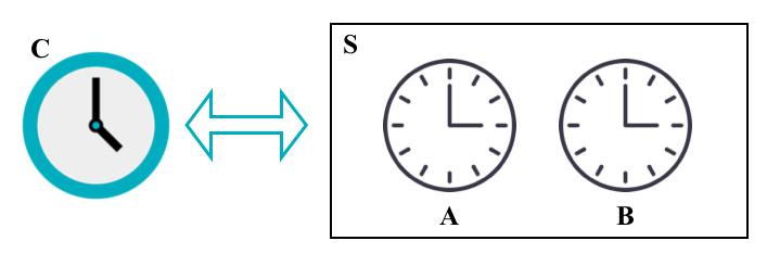
Figure 1: The subsystem $S$ consists of two clocks, $A$ and $B$, and we study their evolution with respect to the clock $C$.

III.1 Evolution of free clocks

As mentioned, we consider here the system $S$ consisting of two clocks $A$ and $B$. The global space is $\mathcal{H}=\mathcal{H}_{C}\otimes\mathcal{H}_{S}=\mathcal{H}_{C}\otimes\mathcal{H}_{A}\otimes\mathcal{H}_{B}$ where we assume $d_{A}=d_{B}=d$ and $d_{C}\gg d$. For the global Hamiltonian we have:

$$\hat{H}=\hat{H}_{C}+\hat{H}_{A}+\hat{H}_{B}$$ (9)

where

$$\hat{H}_{A}=\hat{H}_{B}=\sum_{k=0}^{d-1}\frac{2\pi}{T}k\ket{k}\bra{k}$$ (10)

with

$$\frac{2\pi}{T}k=E^{(A)}_{k}=E^{(B)}_{k}$$ (11)

the equally-spaced energy eigenvalues. We introduce the operators $\hat{\tau}=\sum_{m=0}^{d-1}\tau_{m}\ket{\tau_{m}}\bra{\tau_{m}}$ and $\hat{\theta}=\sum_{l=0}^{d-1}\theta_{l}\ket{\theta_{l}}\bra{\theta_{l}}$ complement of $\hat{H}_{A}$ and $\hat{H}_{B}$ respectively, with

$$\ket{\tau_{m}}_{A}=\frac{1}{\sqrt{d}}\sum_{k=0}^{d-1}e^{-i\frac{2\pi}{T}k\tau_{m}}\ket{k}_{A}=\frac{1}{\sqrt{d}}\sum_{k=0}^{d-1}e^{-i\frac{2\pi}{d}km}\ket{k}_{A}$$ (12)

and

$$\ket{\theta_{l}}_{B}=\frac{1}{\sqrt{d}}\sum_{k=0}^{d-1}e^{-i\frac{2\pi}{T}k\theta_{l}}\ket{k}_{B}=\frac{1}{\sqrt{d}}\sum_{k=0}^{d-1}e^{-i\frac{2\pi}{d}kl}\ket{k}_{B}$$ (13)

where we have defined: $\tau_{m}=m\frac{T}{d}$ and $\theta_{l}=l\frac{T}{d}$ ($m,l=0,1,2,...,d-1$). The Hermitian operator $\hat{\tau}$ is complement of the Hamilitonian $\hat{H}_{A}$ in the sense that $\hat{H}_{A}$ is generator of shifts in eigenvalues of $\hat{\tau}$ and, viceversa, $\hat{\tau}$ is the generator of energy shifts. The same holds for $\hat{\theta}$ with respect to $\hat{H}_{B}$. The quantity $T$ is the time taken by the clocks to return to their initial state, indeed we have $\ket{\tau_{m}+T}_{A}=\ket{\tau_{m}}_{A}$ and $\ket{\theta_{l}+T}_{B}=\ket{\theta_{l}}_{B}$. We want the clocks $A$ and $B$ to be not correlated, so we assume them in a product state in $S$. The global state $\ket{\Psi}$ satisfying the constraint (1) can be written:

$$\begin{split}\ket{\Psi}&=\frac{1}{T_{C}}\int_{0}^{T_{C}}dt\ket{t}_{C}\otimes\ket{\psi(t)}_{S}=\\ &=\frac{1}{T_{C}}\int_{0}^{T_{C}}dt\ket{t}_{C}\otimes\ket{\varphi(t)}_{A}\otimes\ket{\phi(t)}_{B}\end{split}$$ (14)

where $\ket{\psi(t)}_{S}=\braket{t}{\Psi}=\ket{\varphi(t)}_{A}\otimes\ket{\phi(t)}_{B}$ is the relative state of $S=A+B$ at time $t$, namely the state of $A$ and $B$ conditioned to the reading of $t$ in $C$.

Through the state $\ket{\psi(t)}_{S}$ we can study the time evolution of the clocks $A$ and $B$. For the initial state of the clocks we choose:

$$\ket{\psi(0)}_{S}=\ket{\varphi(0)}_{A}\otimes\ket{\phi(0)}_{B}=\frac{1}{\sqrt{d}}\sum_{k=0}^{d-1}\ket{k}_{A}\otimes\frac{1}{\sqrt{d}}\sum_{n=0}^{d-1}\ket{n}_{B}$$ (15)

namely we consider, at time $t=0$, the clocks $A$ and $B$ to be in the time states $\ket{\tau_{0}=0}_{A}$ and $\ket{\theta_{0}=0}_{B}$. The state of $S$ at generic time $t$ reads:

$$\begin{split}\ket{\psi(t)}_{S}&=\ket{\varphi(t)}_{A}\otimes\ket{\phi(t)}_{B}=\\ &=\frac{1}{d}\sum_{k=0}^{d-1}e^{-i\frac{2\pi}{T}kt}\ket{k}_{A}\otimes\sum_{n=0}^{d-1}e^{-i\frac{2\pi}{T}nt}\ket{n}_{B}\end{split}$$ (16)

indicating the clocks following the Schrödinger evolution. As times $t$ goes on, the clocks “click”all the time states $\ket{\tau_{m}}_{A}$ and $\ket{\theta_{l}}_{B}$ until they reaches $t=T$, thus completing one cycle and returning to their initial state. As expected, the clocks evolve synchronously: considering indeed to be at time $t=m\frac{T}{d}$, we have

$$\ket{\psi(t=m\frac{T}{d})}_{S}=\ket{\varphi(t=m\frac{T}{d})}_{A}\otimes\ket{\phi(t=m\frac{T}{d})}_{B}=\\ =\frac{1}{d}\sum_{k=0}^{d-1}e^{-i\frac{2\pi}{d}km}\ket{k}_{A}\otimes\sum_{n=0}^{d-1}e^{-i\frac{2\pi}{d}nm}\ket{n}_{B}$$ (17)

where $A$ is clicking the $m-th$ state $\ket{\tau_{m}}_{A}$ and also $B$ is clicking its $m-th$ state $\ket{\theta_{m}}_{B}$.

III.2 $A$ and $B$ interacting with the gravitational field

We consider now the case in which clocks $A$ and $B$ are placed within a gravitational potential. In doing this we assume $B$ at a distance $x$ from the center of a spherical mass $M$ and $A$ placed at a distance $x+h$ (see Fig. 2). In the interaction between the clocks and the gravitational potential we consider the Newtonian potential $\phi(x)=-\frac{GM}{x}$, where $G$ is the universal gravitational constant and the coordinate $x$ is treated as a number. In calculating such interaction we promote the mass of the clocks to operator using the mass–energy equivalence: $m_{A}\rightarrow m_{A}+\hat{H}_{A}/c^{2}$ and $m_{B}\rightarrow m_{B}+\hat{H}_{B}/c^{2}$. We assume that the static mass of the clocks is negligibly small compared with the dynamical one and we focus only on the effects due to the internal degrees of freedom. Nevertheless, the fact of considering the contributions given by the static masses would only lead to an unobservable global phase factor in the evolution of the clocks.

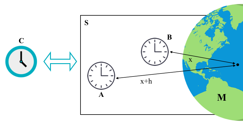
Figure 2: The subsystem $S$ consists of two clocks $A$ and $B$ both placed within the gravitational potential. $B$ is at distance $x$ from the center of the mass $M$, while $A$ is at distance $x+h$.

For the Hamiltonians $\hat{H}_{A}$ and $\hat{H}_{B}$ we have again $\hat{H}_{A}=\hat{H}_{B}=\sum_{k=0}^{d-1}\frac{2\pi}{T}k\ket{k}\bra{k}$, and so the global Hamiltonian is now:

$$\begin{split}\hat{H}&=\hat{H}_{C}+\hat{H}_{A}+\hat{H}_{B}+\frac{\hat{H}_{A}}{c^{2}}\phi(x+h)+\frac{\hat{H}_{B}}{c^{2}}\phi(x)=\\ &=\hat{H}_{C}+\hat{H^{\prime}}_{A}+\hat{H^{\prime}}_{B}\end{split}$$ (18)

where

$$\begin{split}\hat{H^{\prime}}_{A}=\hat{H}_{A}\left(1+\frac{\phi(x+h)}{c^{2}}\right)=\hat{H}_{A}\left(1-\frac{GM}{(x+h)c^{2}}\right)\end{split}$$ (19)

and

$$\hat{H^{\prime}}_{B}=\hat{H}_{B}\left(1+\frac{\phi(x)}{c^{2}}\right)=\hat{H}_{B}\left(1-\frac{GM}{xc^{2}}\right).$$ (20)

The Hamiltonians $\hat{H^{\prime}}_{A}$ and $\hat{H^{\prime}}_{B}$ can be written:

$$\hat{H^{\prime}}_{A}=\sum_{k=0}^{d-1}\frac{2\pi}{T^{\prime\prime}}k\ket{k}\bra{k}$$ (21)

and

$$\hat{H^{\prime}}_{B}=\sum_{k=0}^{d-1}\frac{2\pi}{T^{\prime}}k\ket{k}\bra{k},$$ (22)

where we have defined

$$T^{\prime\prime}=\frac{T}{1-\frac{GM}{(x+h)c^{2}}}$$ (23)

and

$$T^{\prime}=\frac{T}{1-\frac{GM}{xc^{2}}}.$$ (24)

In the subsystem $S$ we introduce again the operators $\hat{\tau}$ and $\hat{\theta}$ which are now complement of $\hat{H^{\prime}}_{A}$ and $\hat{H^{\prime}}_{B}$ respectively. For the time states of the clocks we have:

$$\ket{\tau_{m}}_{A}=\frac{1}{\sqrt{d}}\sum_{k=0}^{d-1}e^{-i\frac{2\pi}{T^{\prime\prime}}k\tau_{m}}\ket{k}_{A}$$ (25)

with

$$\tau_{m}=m\frac{T^{\prime\prime}}{d}=m\frac{T}{d(1-\frac{GM}{(x+h)c^{2}})}$$ (26)

and

$$\ket{\theta_{l}}_{B}=\frac{1}{\sqrt{d}}\sum_{k=0}^{d-1}e^{-i\frac{2\pi}{T^{\prime}}k\theta_{l}}\ket{k}_{B}$$ (27)

with

$$\theta_{l}=l\frac{T^{\prime}}{d}=l\frac{T}{d(1-\frac{GM}{xc^{2}})}.$$ (28)

We notice that the presence of the gravitational field does not change the form of the time states. Indeed, through (26) and (28), we can rewrite (25) and (27) as

$$\ket{\tau_{m}}_{A}=\frac{1}{\sqrt{d}}\sum_{k=0}^{d-1}e^{-i\frac{2\pi}{d}km}\ket{k}_{A}$$ (29)

and

$$\ket{\theta_{l}}_{B}=\frac{1}{\sqrt{d}}\sum_{k=0}^{d-1}e^{-i\frac{2\pi}{d}kl}\ket{k}_{B}$$ (30)

which are the same of (12) and (13). The global state satisfying the global constraint (1) can again be written as in (14) and we assume also here the clocks starting in the product state of $\ket{\tau_{0}=0}_{A}$ and $\ket{\theta_{0}=0}_{B}$.

We can now look at the state $\ket{\psi(t)}_{S}$, exploring the time evolution of $A$ and $B$. At generic time $t$ we have:

$$\begin{split}&\ket{\psi(t)}_{S}=\ket{\varphi(t)}_{A}\otimes\ket{\phi(t)}_{B}=\\ &=\frac{1}{d}\sum_{k=0}^{d-1}e^{-i\frac{2\pi}{T}kt(1-\frac{GM}{(x+h)c^{2}})}\ket{k}_{A}\otimes\sum_{n=0}^{d-1}e^{-i\frac{2\pi}{T}nt(1-\frac{GM}{xc^{2}})}\ket{n}_{B}.\end{split}$$ (31)

Equation (31) shows again the Schrödinger evolution for $A$ and $B$ where we can notice a different delay in the phases of the two clocks. This different delay indicates the two clocks ticking different time states, given a certain time $t$ as read by the clock $C$. This can be seen by considering to be at time $t=m\frac{T}{d}$ as read by $C$. Equation (31) becomes:

$$\ket{\psi(t=m\frac{T}{d})}_{S}=\ket{\varphi(t=m\frac{T}{d})}_{A}\otimes\ket{\phi(t=m\frac{T}{d})}_{B}=\\ =\frac{1}{d}\sum_{k=0}^{d-1}e^{-i\frac{2\pi}{d}km(1-\frac{GM}{(x+h)c^{2}})}\ket{k}_{A}\otimes\sum_{n=0}^{d-1}e^{-i\frac{2\pi}{d}nm(1-\frac{GM}{xc^{2}})}\ket{n}_{B}$$ (32)

showing that neither $A$ nor $B$ have clicked the $m-th$ state. Clock $B$ has indeed clicked a number of states $m^{\prime}=m\left(1-\frac{GM}{xc^{2}}\right)$ and $A$ has clicked a number of states $m^{\prime\prime}=m\left(1-\frac{GM}{(x+h)c^{2}}\right)$ ($m^{\prime},m^{\prime\prime}\in\mathbb{R}$). From this we can derive:

$$\begin{split}m^{\prime}=m^{\prime\prime}\left(1-\frac{GM}{xc^{2}}\right)\left(1-\frac{GM}{(x+h)c^{2}}\right)^{-1}\end{split}$$ (33)

which is in agreement with the time dilation between two clocks at a (radial) distance $h$ from each other as obtained in the first order expansion of the Schwarzschild metric. We notice that the “agreement”only regards the time dilation effect: the $x$ and $x+h$ coordinates represent here simply the distance between the clocks and the center of the spherical mass $M$. We do not define the Schwarzschild radial coordinate, as we do not define coordinate time and proper time. We are indeed working in a purely quantum non-relativistic framework, with the only exception of having promoted the masses of the clocks to operators using the mass-energy equivalence. Expanding the second term in the right-hand side of (33) and neglecting terms $\sim\left(\frac{GM}{xc^{2}}\right)^{2}$, the equation reads

$$\begin{split}m^{\prime}&\simeq m^{\prime\prime}\left(1-\frac{GM}{xc^{2}}\right)\left(1+\frac{GM}{(x+h)c^{2}}\right)=\\ &\simeq m^{\prime\prime}\left(1-\frac{GMh}{x(x+h)c^{2}}\right)\end{split}$$ (34)

which, for $h\ll x$, becomes:

$$m^{\prime}\simeq m^{\prime\prime}\left(1-\frac{ah}{c^{2}}\right)$$ (35)

where we have written the gravitational acceleration as $a=\frac{GM}{x^{2}}$. This time dilation effect is in agreement with the relativistic result in the case, for example, of two clocks placed on the earth and separated by a vertical distance $h$, sufficiently small relative to the radius of the planet. We notice here that our results follows from having a finite $T$. If we consider indeed clocks with unbounded time states, we would not find the same effect.

We can also calculate the gravitational redshift as produced by our framework. We write the frequecy $\nu$ as proportional to the spacing between two neighboring energy levels of the clocks, that is $\nu=1/T$ for a free clock. When $A$ and $B$ are placed within the gravitational field we have:

$$\delta\nu=\nu_{A}-\nu_{B}=\frac{1}{T^{\prime\prime}}-\frac{1}{T^{{}^{\prime}}}$$ (36)

that, for $h\ll x$, becomes

$$\begin{split}\delta\nu&=\frac{1}{T}\left[\left(1-\frac{GM}{(x+h)c^{2}}\right)-\left(1-\frac{GM}{xc^{2}}\right)\right]\\ &=\frac{1}{T}\frac{GM}{c^{2}}\left(\frac{1}{x}-\frac{1}{x+h}\right)\simeq\frac{1}{T}\frac{GMh}{x^{2}c^{2}}.\end{split}$$ (37)

Writing again $a=\frac{GM}{x^{2}}$ and neglecting terms $\sim\left(\frac{GM}{xc^{2}}\right)^{2}$, we obtain

$$\frac{\delta\nu}{\nu_{B}}\simeq\frac{ah}{c^{2}}$$ (38)

that is in agreement with the relativistic result up to the first order of approximation misuragravita . Equation (38) clearly holds also by considering any two energy levels and not two neighbors.

As a last point, we consider the clock $B$ again placed within the gravitational potential at a distance $x$ from origin of the gravitational field, but we bring clock $A$ at an infinite distance from $M$. We implement this scenario simply by taking $h\longrightarrow\infty$. In this limiting case the Hamiltonian of clock $A$ becomes $\hat{H^{\prime}}_{A}\longrightarrow\hat{H}_{A}=\sum_{k=0}^{d-1}\frac{2\pi}{T}k\ket{k}\bra{k}$ and equation (33) reduces to:

$$m^{\prime}=m^{\prime\prime}\left(1-\frac{GM}{xc^{2}}\right).$$ (39)

This expression is again in agreement with the first order expansion ofthe gravitational time dilation as derived from the Schwarzschild metric.

IV Clocks $A$ and $B$ with Continuous Time Values

We replicate here the discussion made in Section III, but considering the clocks $A$ and $B$ represented by Pegg’s POVM with continuous time values. As in the previous Section, we first study the time evolution of free clocks, then we will introduce the gravitational field.

IV.1 Evolution of free clocks

The system $S$ consists here of two free clocks $A$ and $B$ with continuos time values. The global Hilbert space is $\mathcal{H}=\mathcal{H}_{C}\otimes\mathcal{H}_{S}=\mathcal{H}_{C}\otimes\mathcal{H}_{A}\otimes\mathcal{H}_{B}$ where we assume $d_{A}=d_{B}=d$ and $d_{C}\gg d$. For the global Hamiltonian we have:

$$\hat{H}=\hat{H}_{C}+\hat{H}_{A}+\hat{H}_{B}$$ (40)

where

$$\hat{H}_{A}=\hat{H}_{B}=\sum_{k=0}^{d-1}\frac{2\pi}{T}k\ket{k}\bra{k}$$ (41)

with $\frac{2\pi}{T}k=E^{(A)}_{k}=E^{(B)}_{k}$ the equally-spaced energy eigenvalues. In this paragraph we don not consider the Hermitian operators $\hat{\tau}$ and $\hat{\theta}$ complement of $\hat{H}_{A}$ and $\hat{H}_{B}$. Rather we introduce the time states:

$$\ket{\tau_{f}}_{A}=\sum_{k=0}^{d-1}e^{-i\frac{2\pi}{T}k\tau_{f}}\ket{k}_{A}=\sum_{k=0}^{d-1}e^{-i2\pi kf}\ket{k}_{A}$$ (42)

and

$$\ket{\theta_{g}}_{B}=\sum_{k=0}^{d-1}e^{-i\frac{2\pi}{T}k\theta_{g}}\ket{k}_{B}=\sum_{k=0}^{d-1}e^{-i2\pi kg}\ket{k}_{B}$$ (43)

where we have defined $\tau_{f}=fT$ and $\theta_{g}=gT$, with $f$ and $g$ taking any real values in the interval $\left[0,1\right]$. Assuming the clocks $A$ and $B$ in a product state in $S$, the global state $\ket{\Psi}$ satisfying the constraint (1) can again be written:

$$\begin{split}\ket{\Psi}&=\frac{1}{T_{C}}\int_{0}^{T_{C}}dt\ket{t}_{C}\otimes\ket{\psi(t)}_{S}=\\ &=\frac{1}{T_{C}}\int_{0}^{T_{C}}dt\ket{t}_{C}\otimes\ket{\varphi(t)}_{A}\otimes\ket{\phi(t)}_{B}\end{split}$$ (44)

where $\ket{\psi(t)}_{S}=\braket{t}{\Psi}=\ket{\varphi(t)}_{A}\otimes\ket{\phi(t)}_{B}$ is the relative state of $S=A+B$ at time $t$, namely the state of $A$ and $B$ conditioned on the reading $t$ in $C$.

Through $\ket{\psi(t)}_{S}$ we investigate again the time evolution of the clocks $A$ and $B$. For the initial state of the clocks we choose:

$$\ket{\psi(0)}_{S}=\ket{\varphi(0)}_{A}\otimes\ket{\phi(0)}_{B}=\frac{1}{d}\sum_{k=0}^{d-1}\ket{k}_{A}\otimes\sum_{n=0}^{d-1}\ket{n}_{B}$$ (45)

namely we consider, at time $t=0$, the clocks $A$ and $B$ to be in the time states $\ket{\tau_{f=0}}_{A}$ and $\ket{\theta_{g=0}}_{B}$ (apart from a normalization constant). This implies that the state of $S$ at time $t=fT$ is:

$$\ket{\psi(t=fT)}_{S}=\ket{\varphi(t=fT)}_{A}\otimes\ket{\phi(t=fT)}_{B}=\\ =\frac{1}{d}\sum_{k=0}^{d-1}e^{-i2\pi kf}\ket{k}_{A}\otimes\sum_{n=0}^{d-1}e^{-i2\pi nf}\ket{n}_{B}$$ (46)

indicating the clocks evolving synchronously. Indeed, also in this case, we can see $A$ and $B$ clicking simultaneously the time states $\ket{\tau_{f}}_{A}$ and $\ket{\theta_{f}}_{B}$.

IV.2 $A$ and $B$ interacting with the gravitational field

We consider now the case of clocks $A$ and $B$ with continuous time values interacting with the Newtonian gravitaional field. Clock $B$ is placed at a distance $x$ from the center of the mass $M$, while $A$ is at a distance $x+h$. We have again $\hat{H}_{A}=\hat{H}_{B}=\sum_{k=0}^{d-1}\frac{2\pi}{T}k\ket{k}\bra{k}$, and so the global Hamiltonian reads:

$$\begin{split}\hat{H}&=\hat{H}_{C}+\hat{H}_{A}+\frac{\hat{H}_{A}}{c^{2}}\phi(x+h)+\hat{H}_{B}+\frac{\hat{H}_{B}}{c^{2}}\phi(x)=\\ &=\hat{H}_{C}+\hat{H^{\prime}}_{A}+\hat{H^{\prime}}_{B}\end{split}$$ (47)

where

$$\hat{H^{\prime}}_{A}=\hat{H}_{A}\left(1-\frac{GM}{(x+h)c^{2}}\right)=\sum_{k=0}^{d-1}\frac{2\pi}{T^{\prime\prime}}k\ket{k}\bra{k}$$ (48)

and

$$\hat{H^{\prime}}_{B}=\hat{H}_{B}\left(1-\frac{GM}{xc^{2}}\right)=\sum_{k=0}^{d-1}\frac{2\pi}{T^{\prime}}k\ket{k}\bra{k}$$ (49)

with $T^{\prime\prime}=T/(1-\frac{GM}{(x+h)c^{2}})$ and $T^{\prime}=T/(1-\frac{GM}{xc^{2}})$. As in the previous Section, we notice that the presence of the gravitational field does not change the form of the time states for $A$ and $B$. Indeed we have:

$$\ket{\tau_{f}}_{A}=\sum_{k=0}^{d-1}e^{-i\frac{2\pi}{T^{\prime\prime}}k\tau_{f}}\ket{k}_{A}=\sum_{k=0}^{d-1}e^{-i2\pi kf}\ket{k}_{A}$$ (50)

and

$$\ket{\theta_{g}}_{B}=\sum_{k=0}^{d-1}e^{-i\frac{2\pi}{T^{\prime}}k\theta_{g}}\ket{k}_{B}=\sum_{k=0}^{d-1}e^{-i2\pi kg}\ket{k}_{B}$$ (51)

where now $\tau_{f}=fT^{\prime\prime}$ and $\theta_{g}=gT^{\prime}$ with $f,g\in\left[0,1\right]$. The time states (50) and (51) are therefore the same as in the case of free clocks (42) and (43).

We choose the product state (45) as initial condition for the clocks, we can look at the evolution of $A$ and $B$. Assuming clock $C$ to be in $t=fT$, equation (46) becomes:

$$\ket{\psi(t=fT)}_{S}=\ket{\varphi(t=fT)}_{A}\otimes\ket{\phi(t=fT)}_{B}=\\ =\frac{1}{d}\sum_{k=0}^{d-1}e^{-i2\pi kf(1-\frac{GM}{(x+h)c^{2}})}\ket{k}_{A}\otimes\sum_{n=0}^{d-1}e^{-i2\pi nf(1-\frac{GM}{xc^{2}})}\ket{n}_{B}.$$ (52)

Equation (52) shows that, when time $t=fT$ is read by the clock $C$, clocks $A$ and $B$ have not reached the states $\ket{\tau_{f}}_{A}$ and $\ket{\theta_{f}}_{B}$. Rather $A$ is clicking the state $\ket{\tau_{f^{\prime\prime}}}_{A}$ with $f^{\prime\prime}=f\left(1-\frac{GM}{(x+h)c^{2}}\right)$ and $B$ is clicking the state $\ket{\theta_{f^{\prime}}}_{B}$ with $f^{\prime}=f\left(1-\frac{GM}{xc^{2}}\right)$. This implies

$$f^{\prime}=f^{\prime\prime}\left(1-\frac{GM}{xc^{2}}\right)\left(1-\frac{GM}{(x+h)c^{2}}\right)^{-1}$$ (53)

which is the same of equation (33) in this new case of clocks with continuous time values. As we did in Section III.B, neglecting terms of the order $\sim\left(\frac{GM}{xc^{2}}\right)^{2}$, writing the gravitational acceleration $a=\frac{GM}{x^{2}}$ and for $h\ll x$, we can derive:

$$f^{\prime}\simeq f^{\prime\prime}\left(1-\frac{ah}{c^{2}}\right)$$ (54)

where we can see the clock $B$ ticking slower then clock $A$ in agreement with the relativistic result.

Also in this case, the result obtained in Section III.B regarding gravitational redshift can be derived. The spectrum of the clock Hamiltonians has indeed not changed, and we can still define the frequency $\nu=1/T$ for a non-perturbed clock. For the clocks $A$ and $B$ within the gravitational field we have again:

$$\frac{\delta\nu}{\nu_{B}}=\frac{\nu_{A}-\nu_{B}}{\nu_{B}}\simeq\frac{ah}{c^{2}}$$ (55)

where $\nu_{A}=1/T^{\prime\prime}$, $\nu_{B}=1/T^{\prime}$ and $a$ the gravitational acceleration at the distance $x$ from the center of the planet.

Bringing now clock $A$ at infinite distance from $M$ ($h\longrightarrow\infty$), we have again $\hat{H^{\prime}}_{A}\longrightarrow\hat{H}_{A}=\sum_{k=0}^{d-1}\frac{2\pi}{T}k\ket{k}\bra{k}$ and equation (53) becomes:

$$f^{\prime}=f^{\prime\prime}\left(1-\frac{GM}{xc^{2}}\right).$$ (56)

Again we found clock $B$ ticking slower in agreement with the first order expansion of the gravitational time dilation as derived from the Schwarzschild metric.

V Discussion

Our framework leads to the agreement with the Taylor expansion of the Schwarzschild metric up to the first order of approximation. Nevertheless, we can extend our analysis considering the introduction of the relativistic gravitational potential within the global Hamiltonian. Indeed, in this case, the potential energy $V$ of a clock placed at a distance $x$ from the center of the mass $M$ reads gravpot1 ; gravpot2 : $V=m_{clock}c^{2}\left[\left(1-\frac{2GM}{xc^{2}}\right)^{\frac{1}{2}}-1\right]$. Therefore, considering the case of $A$ and $B$ within the field, at distances $x+h$ and $x$ respectively from the origin of the field, and promoting the mass of the clocks to operator using the mass-energy equivalence, we obtain for the global Hamiltonian:

$$\begin{split}\hat{H}&=\hat{H}_{C}+\hat{H}_{A}\left(1-\frac{2GM}{(x+h)c^{2}}\right)^{\frac{1}{2}}+\hat{H}_{B}\left(1-\frac{2GM}{xc^{2}}\right)^{\frac{1}{2}}=\\ &=\hat{H}_{C}+\hat{H^{\prime}}_{A}+\hat{H^{\prime}}_{B}\end{split}$$ (57)

where now

$$\hat{H^{\prime}}_{A}=\hat{H}_{A}\left(1-\frac{2GM}{(x+h)c^{2}}\right)^{\frac{1}{2}}=\sum_{k=0}^{d-1}\frac{2\pi}{T^{\prime\prime}}k\ket{k}\bra{k}$$ (58)

and

$$\hat{H^{\prime}}_{B}=\hat{H}_{B}\left(1-\frac{2GM}{xc^{2}}\right)^{\frac{1}{2}}=\sum_{k=0}^{d-1}\frac{2\pi}{T^{\prime}}k\ket{k}\bra{k}$$ (59)

with $T^{\prime\prime}=T\left(1-\frac{2GM}{(x+h)c^{2}}\right)^{-\frac{1}{2}}$ and $T^{\prime}=T\left(1-\frac{2GM}{xc^{2}}\right)^{-\frac{1}{2}}$.

We can now investigate the time evolution of $A$ and $B$. When the clock $C$ reads the generic time $t$, we have:

$$\begin{split}&\ket{\psi(t)}_{S}=\ket{\varphi(t)}_{A}\otimes\ket{\phi(t)}_{B}=\\ &\propto\sum_{k=0}^{d-1}e^{-i\frac{2\pi}{T}kt(1-\frac{2GM}{(x+h)c^{2}})^{\frac{1}{2}}}\ket{k}_{A}\otimes\sum_{n=0}^{d-1}e^{-i\frac{2\pi}{T}nt(1-\frac{2GM}{xc^{2}})^{\frac{1}{2}}}\ket{n}_{B}.\end{split}$$ (60)

In the case of clocks with discrete time values equation (60) implies that, when $A$ clicks its $m^{\prime\prime}-th$ time state, clock $B$ has clicked a number of states:

$$m^{\prime}=m^{\prime\prime}\left(1-\frac{2GM}{xc^{2}}\right)^{\frac{1}{2}}\left(1-\frac{2GM}{(x+h)c^{2}}\right)^{-\frac{1}{2}}$$ (61)

which, for $h\longrightarrow\infty$, becomes $m^{\prime}=m^{\prime\prime}\left(1-\frac{2GM}{xc^{2}}\right)^{\frac{1}{2}}$. In the same way, when considering clocks with continuous time values, equation (60) implies that, when $A$ clicks the time state $\ket{\tau_{f^{\prime\prime}}}_{A}$, the clock $B$ is clicking the time state $\ket{\theta_{f^{\prime}}}_{B}$ with:

$$f^{\prime}=f^{\prime\prime}\left(1-\frac{2GM}{xc^{2}}\right)^{\frac{1}{2}}\left(1-\frac{2GM}{(x+h)c^{2}}\right)^{-\frac{1}{2}}$$ (62)

which, in the limit $h\longrightarrow\infty$, becomes $f^{\prime}=f^{\prime\prime}\left(1-\frac{2GM}{xc^{2}}\right)^{\frac{1}{2}}$. Therefore, introducing the relativistic gravitational potential, we obtain a time dilation in agreement with the exact Schwarzschild solution.

VI Conclusions

In this work we have explored the effects of gravity on quantum clocks. We have considered two clocks, $A$ and $B$, interacting with a Newtonian gravitational field, and we have studied their evolution with respect to the clock $C$, taken as a far-away reference via the PaW mechanism. We have performed our investigation in the case of $A$ and $B$ having discrete and continuous time values.

In both cases we have first considered two free clocks and shown that, as expected, they evolve synchronously over time. Then we have studied the scenario in which the clocks are placed in the gravitational field, at different distances from the origin of the field. We have shown that, as time $t$ goes on (as read by the far-away clock $C$), the states of the two clocks suffer a different delay in the phases depending on the intensity of the gravitational potential. This delay in the phases translates into the two clocks ticking at different rates. The time dilation is in accordance with the first order expansion of the gravitational time dilation as derived from the Schwarzschild metric. Finally, we have discussed the possibility of using the relativistic gravitational potential within the global Hamiltonian and we have shown that this choice leads to the agreement between our time dilation effect and the exact result obtained with the Schwarzschild metric.