Reverse-time analysis and boundary classification of directional biological dynamics with multiplicative noise

Abstract

The dynamics of living systems often serves the purpose of reaching functionally important target states. We previously proposed a theory to analyze stochastic biological dynamics evolving towards target states in reverse time. However, a large class of systems in biology can only be adequately described using state-dependent noise, which had not been discussed. For example, in gene regulatory networks, biochemical signaling networks or neuronal circuits, count fluctuations are the dominant noise component. We characterize such dynamics as an ensemble of target state aligned (TSA) trajectories and characterize its temporal evolution in reverse-time by generalized Fokker-Planck and stochastic differential equations with multiplicative noise. We establish the classification of boundary conditions for target state modeling for a wide range of power law dynamics, and derive a universal low-noise approximation of the final phase of target state convergence. Our work expands the range of theoretically tractable systems in biology and enables novel experimental design strategies for systems that involve target states.

I INTRODUCTION

The dynamics of living and cognitive systems often serves the purpose of reaching functionally important target states[1, 2, 3, 4, 5, 6, 7, 8, 9, 10, 11, 12, 13, 14, 15, 16, 17, 18, 15, 19, 20]. In the dynamics of decision-making, in morphogenesis, or in cell fate determination for instance, reaching the target state terminates the respective dynamical state and irreversibly commits the system to a novel action or dynamical state. The fact that such target states in a given system are reached only once poses interesting challenges for the data-driven identification and the mathematical modeling of target-state-directed dynamics.

In Lenner et al. [21] we developed a mathematical formalism to describe and infer such dynamics in reverse time, following the dynamics from the time of target state arrival into the past and measuring time as ”time to completion”. We derived and characterized reverse-time Fokker-Planck and stochastic differential equations for target-state-aligned (TSA) ensembles, showed that they exhibit distinct types of universal behavior during target state convergences, and showed that this formalism enables the precise identification of the dynamical laws of target state convergence from ensemble measurements.

In a wide class of biological systems, including gene regulatory networks, biochemical signaling networks or neuronal circuits for instance, count fluctuations are the dominant noise component, which in stochastic dynamics models is best described by state-dependent, ”multiplicative” noise terms[22, 23, 24, 25, 26]. To analyze and model target-state-directed dynamics in such systems, we here develop a theory for reverse-time stochastic dynamics and TSA ensembles for systems with state-dependent noise. We characterize TSA ensembles under multiplicative noise by generalized Fokker-Planck and stochastic differential equations in reverse time, establish the classification of boundary conditions for target state modeling for a wide range of power law dynamics, and derive a universal low-noise approximation of the final phase of target state convergence.

II MATHEMATICAL FORMULATION OF TIME REVERSAL AND TARGET STATE ALIGNMENT

In this study, we examine the temporal evolution of a target state directed variable $\widehat{L}$ subject to both deterministic and random forcing. In the overdamped limit a Langevin equation (Ito interpretation [27])

$$d\widehat{L}=f(\widehat{L})dt+\sqrt{D(\widehat{L})}\;dW_{t}$$ (1)

captures such dynamics. In our notation $\widehat{L}$ denotes a variable evolving in the usual forward time while $L$ stands for a variable that evolves in reverse time, which is introduced below. $f(\widehat{L})$ is a continuous function of $\widehat{L}$ and denotes the deterministic contribution to the force. $D(\widehat{L})$ is a position dependent diffusion ”constant” and a continuous function as well. The Wiener increment implies that the noise is delta correlated with $D(\widehat{L})\langle dW_{t}dW_{t^{\prime}}\rangle=D(\widehat{L})\delta(t-t^{\prime})dt$. The dynamics is assumed to originate from a distribution $P^{\mathrm{in}}(\widehat{L})=P(\widehat{L}_{0},t_{0})$. The target state is defined as $\widehat{L}_{\mathrm{ts}}$ and mathematically corresponds to an absorbing boundary condition. An exemplary realization of Eq. (1) is shown in Fig. 1.

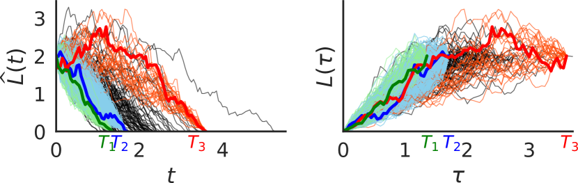
Figure 1: Construction of the aligned time reversed ensemble from sub-ensembles of different lifetimes. (Left): The full forward ensemble is split into sub-ensembles with different completion times $T_{i}$. We show three exemplary cases in green ($T_{1}$), blue ($T_{2}$) and red ($T_{3}$). To guide the eye, one sample path per sub-ensemble is highlighted. (Right): After target state alignment and time reversal all sub-ensembles together form the new ensemble $P(L,\tau)$.

The mathematical formulation of target state alignment and time reversal of ensembles generated by Eq. (1) is an intricate problem. The construction idea is as follows (see Fig. 1):

I) In the first step we partition the forward ensemble into sub–ensembles. Each sub-ensemble $E_{i}$ contains only sample paths which reach the target state in the temporal interval $\left[T_{i},T_{i}+\Delta T\right]$. The time $T_{i}$ is itself a stochastic variable which is distributed according to the hitting time distribution.

II) In the second step, we revert the direction of time for each sub–ensemble. The mathematical formalism that allows the time-reversal of ensembles of identical temporal extension $T_{i}$ is called the reverse–time Fokker–Planck equation or equivalency the reverse–time Langevin equation [28]. For multiplicative noise the latter can be written as

$$dL=\bigg{(} -f(L)$$

$$+D(L)\frac{\partial}{\partial L}\log\left(D(L)P^{\mathrm{fw}}(L,T-\tau)\right)\bigg{)}d\tau$$

$$+\sqrt{D(L)}\;dW_{\tau}$$ (2)

in Ito interpretation. Note that $L$ is missing the hat now and we introduced the reverse time $\tau$. $P^{\mathrm{fw}}(L,T-\tau)$ is the probability density of the forward process with ”fixed” forward hitting time $T$ and $\tau$ starting from zero. Hence, the initial conditions of this reverse-time dynamic are the target state $(L_{\mathrm{ts}},\tau_{0})$ and the final state is the initial state of the forward process $(L_{f},\tau_{f})=(\widehat{L}_{0},t_{0})$. We denote the probability distribution which solves the corresponding Fokker-Planck equation as $R(L,\tau|T;L_{f})$. Initial conditions at the target state are implied.

III) In the last step we stitch these time–reversed sub–ensembles together to form the full TSA ensemble. The alignment is achieved by choosing the same initial times $\tau_{0}$ for each time–reversed sub–ensemble. Each sub–ensemble is already normalized by construction. To achieve normalization in the full TSA ensemble, each sub–ensemble must be re-weighted with the hitting time distribution, the measure which counts how many trajectories are in one bin $\left[T_{i},T_{i}+\Delta T\right]$. The full TSA ensemble then reads

$$R(L,\tau) =$$

$$=\int_{L_{\mathrm{ts}}}^{\infty} dL_{f}P^{\mathrm{in}}(L_{f})\int_{\tau}^{\infty}dT\ R(L,\tau|T;L_{f})\rho(T|L_{f})\ \ ,$$ (3)

where we set $\tau_{0}=0$. In addition, we averaged the expression with respect to the initial value distribution $P^{\mathrm{in}}(L_{f})$ of the forward process.

The temporal evolution of Eq. (II) can be obtained by taking the partial derivative of Eq. (II) with respect to the reverse time $\tau$. After some transformations, detailed in the supplementary information, we obtain a Fokker-Planck equation with a sink term proportional to the hitting time distribution. The corresponding Langevin equation in Ito representation reads

$$dL(\tau)=\Bigg{(}f(L)+$$

$$D(L)\ \frac{\partial}{\partial L}\log\left(\int_{L_{\mathrm{ts}}}^{L}dL^{\prime}\;e^{-\int^{L^{\prime}}\frac{2f(L^{\prime\prime})}{D(L^{\prime\prime})}dL^{\prime\prime}}H(L^{\prime})\right)\Bigg{)}d\tau$$

$$+\sqrt{D(L)}\ dW_{\tau}$$ (4)

with

$$H(L^{\prime})=\left(1-\int_{L_{\mathrm{ts}}}^{L^{\prime}}P^{\mathrm{in}}(L^{\prime\prime})dL^{\prime\prime}\right)$$ (5)

and killing measure [29, 30, 31]

$$k(L,\tau)=\frac{P^{\mathrm{in}}(L)\rho_{L_{\mathrm{ts}}}(\tau|L)}{R_{L_{\mathrm{ts}}}(L,\tau;\tau_{0})}\ .$$ (6)

The latter is responsible to terminate trajectories proportional to the hitting time distribution. The term $H(L)$ denotes the dependence on the initial conditions

For dynamics with target states sufficiently far from the initial conditions ($H(L)=1)$, and temporally well separated from the start of the forward dynamics $(k(L,\tau)=0)$, the Langevin equation simplifies to an initial value problem.

In the vicinity of target states, here chosen as $L_{\mathrm{ts}}=0$, we can expand both the force law and the noise in power laws. Keeping only the terms of lowest order, the forward Langevin equation reads

$$d\widehat{L}=-\gamma\widehat{L}^{\alpha}dt+\sqrt{D\widehat{L}^{\beta}}\;dW_{t}\ .$$ (7)

III FELLER BOUNDARY CLASSIFICATION

Unlike for constant noise dynamics with target state directed forces ($\gamma>0\ ,\beta=0$) these dynamics are not guaranteed to always reach the target state in on average finite time. This statement can be substantiated using the Feller boundary classification scheme [32, 33, 34].

The Feller boundary classification scheme is based on the formalization of two questions: I) What is the probability of first passage through the boundary? II) What is the average time it takes to get there from an initial state? The answer to these questions, allows to distinguish 4 scenarios: A boundary is called regular, if it can be reached and crossed from both sides in finite time and points in the interval are accessible if starting from the boundary. Exit boundaries can be reached in finite time, but entering the interval from the endpoint is impossible. Entrance boundaries can not be reached in finite time from inside the defining interval but entering the interval is possible if the dynamics starts at the boundary. Natural boundaries can neither be reached nor exited from in finite time. Feller’s scheme is based on a clever mapping of arbitrary one-dimensional stochastic dynamics to the Brownian motion case. This transformation yields four criteria for which the asymptotic behavior is analytically accessible even if it is not possible to find an explicit expression for the transition density [32]. For the Langevin Eq. (8), the different regimes have been calculated (see supplementary information) and are shown in Fig. 2.

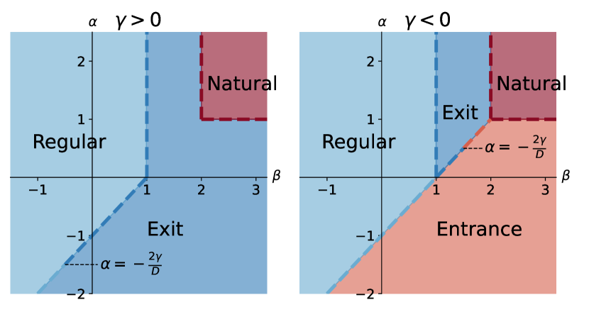
Figure 2: Target states can only be reached by a subset of dynamics with power law like deterministic and random forcing. Feller Boundary classification scheme [32, 34, 35] for the dynamics in Eq. (7) and a target state at $\widehat{L}_{ts}=0$. Blue colors denote regular and exit boundaries, i.e. those cases where the boundary is reached in finite time and red colors denote natural and entrance boundaries, i.e. those cases where the target state can not be reached in finite time. Margins between the phase-regions are assigned dashed lines in the color of its respective boundary class. For a derivation of the boundary classification see the supplementary information, which also gives the definition of the different classes. (Left): Here we consider noise dominated target state approach ($\gamma>0$). The point at $\alpha=-\frac{2\gamma}{D}$ belongs to the exit boundary class. (Right): Here we consider target state directed forces ($\gamma<0$). The point at $\alpha=-\frac{2\gamma}{D}$ belongs to the entrance boundary class, the point at $\alpha=1,\beta=2$ to the natural boundary class and the point at $\alpha=0,\beta=1$ to the exit boundary class.

To our knowledge such a general characterization as a function of exponents $\alpha$ and $\beta$ has not been given previously. Specific choices of $\alpha$ and $\beta$ have been discussed in the literature [36, 35, 37]. In the supplementary information we also include an introduction to the Feller boundary classification scheme, including an intuitive explanation of the boundary classes and criteria.

Dynamics which can reach target states are either equipped with regular boundary conditions or exit boundaries. From Fig. 2 we read off, that dynamics, where the forces point towards the target state ($\gamma>0$), always reach the target state in finite time if neither the spatial derivative of the (deterministic) force nor the spatial derivative of the random force are zero at the boundary (that is e.g. for jointly $\alpha<1$ and $\beta<2$). In simpler words, the boundary is not attainable if the last step towards the boundary is neither deterministically nor stochastically possible, as both terms asymptotically approach zero. If the force points away from the boundary, the random forcing must dominate the deterministic forcing to nevertheless reach the boundary. The boundary is only reached if the noise contribution is at least as large as the force contribution of the last step.

In models with the target state accessible for power law driven dynamics (Eq. (8)), we determined the exact expression for the forces in the TSA reverse-time ensemble using Eq. (II). The reverse-time Langevin equation reads

$$dL(\tau)=\left(-\gamma L^{\alpha}+f^{\mathcal{F}}(L)\right)d\tau+\sqrt{DL^{\beta}}\ dW_{\tau}$$ (8)

$$\mathrm{with}\qquad f^{\mathcal{F}}(L)=$$

$$=L^{\beta}\frac{D(\alpha-\beta+1)\left(-\frac{2\gamma}{D(\alpha-\beta+1)}\right)^{\frac{1}{\alpha-\beta+1}}e^{\frac{2\gamma L^{\alpha-\beta+1}}{D(\alpha-\beta+1)}}}{\Theta(\alpha-\beta+1)\Gamma\left(\frac{1}{\alpha-\beta+1}\right)-\Gamma\left(\frac{1}{\alpha-\beta+1},-\frac{2L^{\alpha-\beta+1}\gamma}{D(\alpha-\beta+1)}\right)}$$

$$\mathrm{valid\ for}\qquad\alpha-\beta\neq-1\ ,$$ (9)

where $\Gamma(z)$ is the gamma-function, $\Gamma\left(\nu,z\right)$ the upper incomplete gamma function and $\Theta(\nu)$ the Heaviside step function.

The case $\alpha-\beta=-1$ is substantially simpler. For this special case the reverse-time Langevin equation becomes

$$dL(\tau)=(\gamma+D)L^{\alpha}d\tau+\sqrt{DL^{\alpha+1}}\ dW_{\tau}\qquad\alpha-\beta=-1\ .$$ (10)

We solved the exact target state aligned reverse time Fokker-Planck equation for the case $\alpha=0,\beta=1$ and present the calculated mean and variance in Fig. 3 (see supplementary information for details).

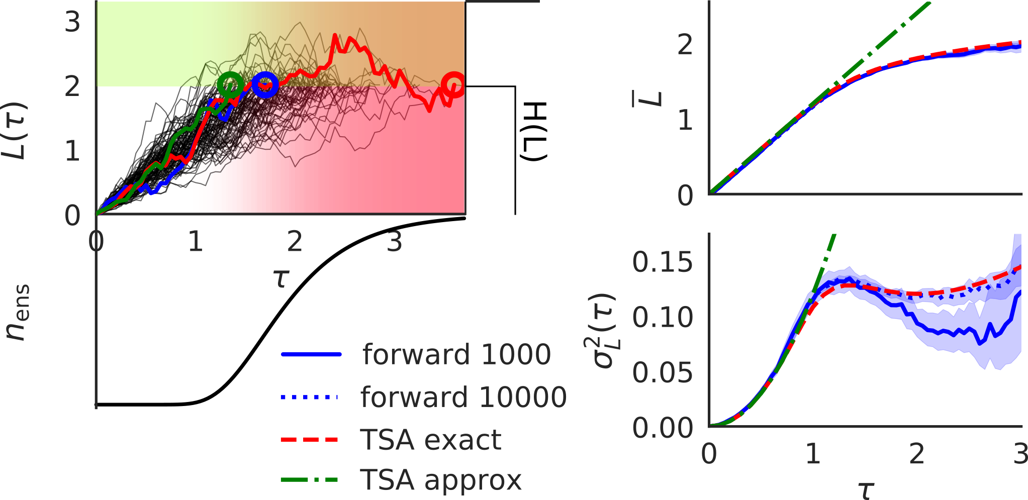
Figure 3: The TSA reverse-time Langevin equation exactly describes the target state aligned ensemble. (Left): Schematic depiction of the dependency of the TSA dynamics Eq. (II) on the forward initial condition $H(L)$ Eq. (5) and the killing measure $k(L,\tau)$ Eq. (6). In the green region, i.e. above the bulk of the initial distribution measured by the sigmoidal $H(L)$, we find $f^{\mathcal{F}}(L)\approx 0$. Below $f^{\mathcal{F}}(L)$ contributes in full strength. In $\tau$ direction, an increase in the red gradient indicates, that more and more trajectories are killed. The residual white $L-\tau$ plane close to the target state defines the region where $k(L,\tau)\approx 0$ and $H(L)=1$ holds, and the approximation of well separated initial and final states holds. Circles mark the killing of example trajectories. (Right): Comparison of the forward (blue), sub-ensemble based (red), exact (black) and approximate (green) reverse-time dynamics for $f(L)=-\gamma/L$. Shown are the mean (Top) and variance (Bottom) of all four cases. 95% bootstrap confidence intervals [38] are shown for the cases involving sampling. To exclude numerical inaccuracies due to rarely visited tails of the distribution of completion times $\rho(T|L_{f})$, we directly sampled $T_{i}$ from the numerically obtained hitting time distribution of the forward process. Results were obtained using each 1000 sample path realizations with parameter settings $\gamma=1$, $D=0.2$, $\widehat{L}_{\mathrm{init}}=2$.

The TSA approximation, valid for dynamics close to target states ($H(L)=1$, no killing measure), can be evaluated for all $\alpha=\beta-1$ ($\beta<2$). We made use of results for Bessel processes [39, 36]. We calculated the mean and variance (see supplementary information) and compare to both the exact result and the mean and variance obtained by forward simulation and subsequent target state alignment and time reversal. The simulations are in excellent agreement with the theoretical expressions (see Fig. 3). The TSA approximation, evaluated analytically with respect to mean and variance, captures the dynamics close to the target state with similar quality (see supplementary information for calculations and Fig. 3). This demonstrates the effectiveness and power of the TSA approximation.

IV UNIVERSAL BEHAVIOR CLOSE TO TARGET STATES

Close to the target state the free energy force (Eq. (III)) can be expanded in low orders of $L$. We find two easily interpretable cases. The reverse-time Langevin equation for power laws (Eq. (8) & Eq. (10)) simplifies to a noise driven ($\alpha\geq\beta$)

$$dL(\tau)=\left(DL^{\beta-1}-\gamma\frac{\alpha-\beta}{\alpha-\beta+2}L^{\alpha}\right)d\tau+\sqrt{D\,L^{\beta}}\ dW_{\tau}$$ (11)

and force driven ($\alpha<\beta$)

$$dL(\tau)=\left(\gamma L^{\alpha}-D(\alpha-\beta)L^{\beta-1}\right)d\tau+\sqrt{D\,L^{\beta}}\ dW_{\tau}$$ (12)

case. Note that the force driven case additionally requires to assume that $D$ is small whenever $-1<\alpha-\beta<0$ holds. Details of both expansions are provided in the supplementary information.

In the noise driven case ($\alpha\geq\beta$), the dynamics are dominated by a power law term that depends on the diffusion constant. For example, in the simple case of multiplicative noise with $\beta=1$, a constant drift term of size $D$ appears which drives the reverse time dynamics away from the target state. In general, the $D$ dependence of the leading order power law in Eq. (11) suggest, that the underlying deterministic force laws are hardly distinguishable in noise driven dynamics close to the target state. We therefore exclusively use the power law term of lowest order which allows us to solve Eq. (11) ($\gamma$ = 0) exactly (see supplementary information). This yields the mean

$$\overline{L}(\tau)=\frac{2^{\frac{\beta-1}{\beta-2}}(2-\beta)^{-\frac{2}{\beta-2}}\Gamma\left(-\frac{2}{\beta-2}\right)}{\Gamma\left(\frac{1}{2-\beta}\right)}(D\tau)^{\frac{1}{2-\beta}}$$ (13)

and the variance

$$\sigma_{L}^{2}(\tau)= (2-\beta)^{-\frac{4}{\beta-2}}\Bigg{(}3\cdot 4^{\frac{1}{\beta-2}}\frac{\Gamma\left(-\frac{3}{\beta-2}\right)}{\Gamma\left(\frac{1}{2-\beta}\right)}$$

$$-4^{\frac{\beta-1}{\beta-2}}\frac{\Gamma\left(-\frac{2}{\beta-2}\right)^{2}}{\Gamma\left(\frac{1}{2-\beta}\right)^{2}}\Bigg{)}(D\tau)^{\frac{1}{1-\beta/2}}\ .$$ (14)

Disregarding the lengthy constants, both mean and variance follow a simple power law in reverse time $\tau$. For constant noise ($\beta=0$), we recover our previous result in [21]. The mean increases as a square root of the time $\tau$, the variance increases linearly with time. In Fig. 4 we compare the three cases $\beta=-1,0,1$. We find excellent agreement of our theory with the corresponding simulations, which were performed in forward time and subsequently aligned to the target state. Interestingly, all three cases ($\beta=-1,0,1$) show a clearly distinguishable behavior in their respective mean and variance. Therefore, this suggests to use the mean and variance of the TSA noise-driven dynamics for system identification for inference from experimental data.

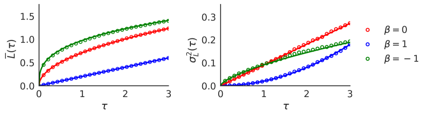
Figure 4: TSA ensembles with dominant multiplicative noise are distinguishable in their mean and variance. Comparison of forward (circles) and exact (lines) multiplicative noise driven TSA dynamics with $f(L)=0$ and $D(L)=DL^{\beta}$ with $\beta=-1,0,1$. Shown are the mean (Left) and variance (Right) for all three cases. The statistics of the forward dynamics are based on 20000 trajectories that start at $\widehat{L}_{0}=20$, to effectively get rid of the initial conditions. The exact analytic expression of reverse time TSA mean and variance are taken from Eq. (13) and Eq. (IV). Parameters were chosen as $\gamma=1$ and $D=0.2$.

In the force driven case ($\alpha<\beta$) the leading order term of the reverse-time Langevin Eq. (12) is the sign inverted forward force term. The diffusion constant $D$ dependent term serves as higher order correction. To obtain closed form expressions for mean, variance and covariance, we expand Eq. (12) in leading orders of $D$ (see supplementary information for details). Using this small noise expansion, we determined the mean

$$\overline{L}(\tau)=((1-\alpha)\gamma t)^{\frac{1}{1-\alpha}}$$

$$+\frac{D}{\gamma}\frac{\left(7\alpha^{2}-\alpha(8\beta+3)+2\beta(\beta+1)\right)((1-\alpha)\gamma\tau)^{\frac{\alpha-\beta}{\alpha-1}}}{2(2\alpha-\beta)(3\alpha-\beta-1)}$$ (15)

and variance

$$\sigma_{L}^{2}(\tau) =\frac{D}{\gamma}\frac{((1-\alpha)\gamma\tau)^{\frac{1-\alpha+\beta}{1-\alpha}}}{1-3\alpha+\beta}$$ (16)

and two time covariance

$$C (\tau,\tau^{\prime})=$$

$$= \begin{cases}D\frac{((1-\alpha)\gamma\tau^{\prime})^{-\frac{\alpha}{\alpha-1}}((1-\alpha)\gamma\tau)^{\frac{-2\alpha+\beta+1}{1-\alpha}}}{\gamma(1-3\alpha+\beta)}&\ \mathrm{for}\ \tau<\tau^{\prime}\\ D\frac{((1-\alpha)\gamma\tau)^{-\frac{\alpha}{\alpha-1}}((1-\alpha)\gamma\tau^{\prime})^{\frac{-2\alpha+\beta+1}{1-\alpha}}}{\gamma(1-3\alpha+\beta)}&\ \mathrm{for}\ \tau>\tau^{\prime}\\ \sigma_{L}^{2}(\tau)&\ \mathrm{for}\ \tau=\tau^{\prime}\ .\end{cases}$$ (17)

up to order $D$.

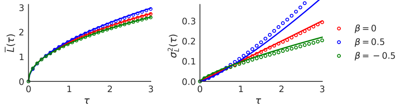
Figure 5: Force dominated TSA dynamics with multiplicative noise are distinguishable in their variance. Comparison of forward (circles) and small noise (lines) TSA expression for dynamics with $f(L)=-\frac{\gamma}{L}$ and multiplicative noise $D(L)=DL^{\beta}$ with $\beta=0,0.5,-0.5$. Shown are the mean (Left) and variance (Right) for all three cases. For the mean the influence of $\beta$ is marginal. For the variance $\beta>0$ leads to an up sloping, $\beta<0$ to a down sloping, and $\beta=0$ to a linear variance. The statistics of the forward dynamics are based on 20000 trajectories that start at $\widehat{L}_{0}=20$. The analytic expressions for the mean and variance are stated in Eq. (IV) and Eq. (16). The parameters are $\gamma=1$ and $D=0.2$.

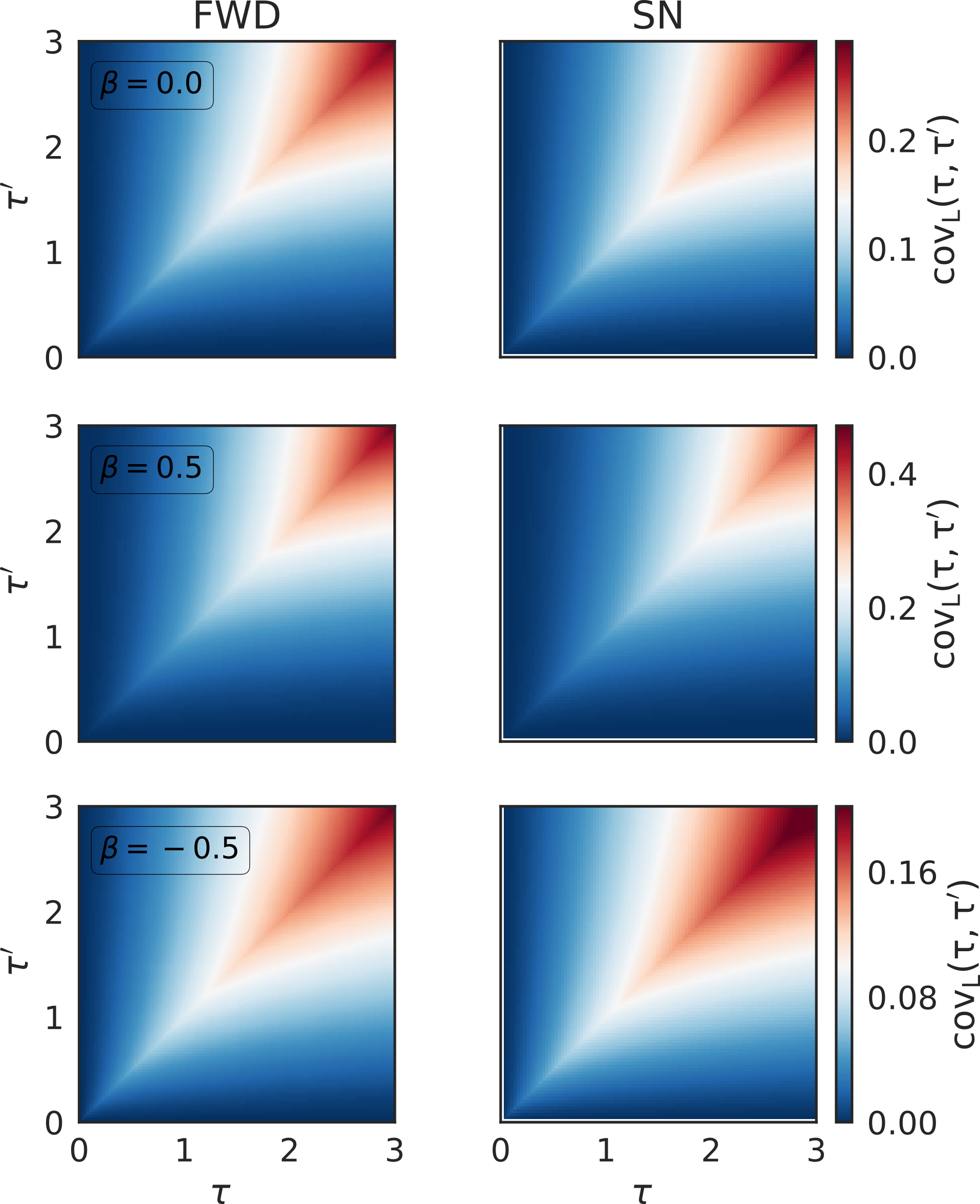
Figure 6: The two-time covariance for force driven dynamics with multiplicative noise can be predicted from a small noise expression. Comparison of the forward (FWD) and reverse time TSA small noise (SN) covariance for $f(L)=-\frac{\gamma}{L}$ and multiplicative noise $D(L)=DL^{\beta}$, with $\beta=0,0.5,-0.5$. The statistics of the forward dynamics are based on 20000 trajectories that start at $\widehat{L}_{0}=20$. The small noise covariance is stated in Eq. (IV). The used parameters are $\gamma=1$ and $D=0.2$.

The above noted small noise results allow us to make some general observations on the behavior of force driven dynamics close to target states. Most telling about the functional characteristics of state dependent noise is the variance. Only for $\beta=0$ the variance of the reverse time ensemble grows linearly with time. For $\beta<0$, the variance is concave close to the target state, for $\beta>0$ it is convex. We show a concrete example for all three cases in Fig. 5. Ensembles generated by forward simulation and subsequent target state alignment are in good agreement with the analytically obtained small noise expression of the variance Eq. (16).

The mean of force driven dynamics is slightly more complicated to characterize. Dependent on the detailed parameter settings, the higher order term in the small noise expansion of the force driven mean can change from concave to convex (Eq. (IV)). Our small noise approximation is perfectly capable to resolve such small changes. We show this for three cases in Fig. 5. Changes in $\beta$ are perfectly resolvable with our higher order correction to the deterministic baseline.

The two-time covariance of force driven dynamics allows for a very visual differentiation between different multiplicative noise regimes. We show three different noise regimes in Fig. 6. For each case, our small noise approximation of the covariance (Eq. (IV)) is in good agreement with the covariance obtained from forward simulated and subsequently target state aligned trajectories.

V DISCUSSION

Typical physics problems prime us to expect dynamical systems problems as initial value problems. Often we can indeed either theoretically or experimentally prepare the system in a well defined initial state and then propagate the dynamics in forward time. In stochastic dynamics we additionally need to account for random forces that perturb the dynamics. But also in stochastic dynamics we already know best how to analyze initial value problems. The temporal evolution of stochastic processes is canonically described by Langevin equations if the focus lies on the generation of individual sample paths and the forward Fokker Planck equation to describe the evolution of the ensemble [40]. Both can be used to describe initial value problems, that is dynamics starting from an initial distribution. In living systems, however, such initial value problems are rare. The biological dynamics we studied above are much better characterized as ”final value” problems reflecting that functional demands require canalization towards target states [1, 2, 3, 4, 5, 6, 7, 8, 9, 10, 11, 12, 13, 14, 15, 16, 17, 18, 15, 19, 20].

Interventions to artificially introduce initial conditions are typically practically inconceivable and would in fact not interrogate the naturally occurring dynamics. We therefore suggested in [21] to analyze end state directed dynamics in their natural frame of reference, that is, in reverse time as a target state aligned ensemble. In our previous study, we showed how such target state aligned (TSA) ensembles can be analyzed for the simpler case of state-independent noise. In the current paper we extend this framework to include general position dependent diffusion, that is multiplicative noise. In this setting, we find target state directed dynamics with much richer behavior close to target states. Including multiplicative noise also expands the applicability of our approach to a new range of problems in finance, neuroscience, chemistry, evolution and cell biology [22, 23, 24, 25, 26].

In the case of constant noise, all dynamics with a force vector pointing towards the target state will eventually reach the target state. For dynamics with multiplicative noise this is not any longer guaranteed. We determined the class of dynamics which on average reach the target state in finite time. We determine the universal form of power laws close to the target states and derive expressions for mean, variance and covariance –both in the noise dominated or force dominated limit. These expressions provide an intuition for possible underlying dynamics in TSA ensembles and form a solid foundation for the data-driven identification of target state directed dynamical systems. Target state alignment is a technique which allows to analyze directional stochastic dynamics with uncontrollable initial conditions. Intriguingly, target states alignment however creates pseudo-forces that have to be separated from the true underlying forward dynamics. Our theory of target state aligned ensembles, allows us to map out the range of inferable TSA dynamics with quantitative precision and principled mathematical controls.