Convergent estimators of variance of a spatial mean in the presence of missing observations

Abstract

In the geosciences, a recurring problem is one of estimating spatial means of a physical field using weighted averages of point observations. An important variant is when individual observations are counted with some probability less than one. This can occur in different contexts: from missing data to estimating the statistics across subsamples. In such situations, the spatial mean is a ratio of random variables, whose statistics involve approximate estimators derived through series expansion. The present paper considers truncated estimators of variance of the spatial mean and their general structure in the presence of missing data. To all orders, the variance estimator depends only on the first and second moments of the underlying field, and convergence requires these moments to be finite. Furthermore, convergence occurs if either the probability of counting individual observations is larger than $1/2$ or the number of point observations is large. In case the point observations are weighted uniformly, the estimators are easily found using combinatorics and involve Stirling numbers of the second kind.

Centre for Atmospheric and Oceanic Sciences and Divecha Centre for Climate Change, Indian Institute of Science, Bangalore 560012, India, email: ashwins@iisc.ac.in

1 Introduction

Very often in the geosciences, we seek estimates of the spatial average of some physical variable such as rainfall or temperature (Rodríguez-Iturbe and Mejía (1974); Shen et al. (1994); Morrissey et al. (1999); Kundu and Siddani (2007); Villarini et al. (2008); Prakash et al. (2019)). Examining the properties of such an average is a decades-old problem (Kagan (1997)). An interesting variant is where individual observations are reported with known probability that is less than one. In this case, what form do the estimators of bias and variance of the spatial average take? Seshadri (2018) examined such a situation, involving point observations $r_{i}$ at locations $i$ $\left(1\leq i\leq N\right)$, with each observation assigned weight $\beta_{i}$, such that $\sum_{i}\beta_{i}=1$. Time is assumed discrete, and not all observations are reported at each time. The reporting status is measured by Boolean random variable $s_{i}$, with $s_{i}=1$ if reported at that time and $s_{i}=0$ otherwise. In our setting, the reporting status of each observation site has been assumed to be independent of whether any other sites, including those in close proximity, are reported. This makes the $s_{i}$’s statistically independent. Assuming that each $s_{i}$ has probability $\alpha$ of equaling one, we define the spatial average over samples without replacement

$$r\left(t\right)\equiv\frac{R\left(t\right)}{S\left(t\right)}=\frac{\sum_{i}\beta_{i}s_{i}\left(t\right)r_{i}\left(t\right)}{\sum_{i}\beta_{i}s_{i}\left(t\right)},$$ (1)

which describes the weighted mean over only those observations that are reported. The weights $\beta_{i}$ are constant in time, but $s_{i}$ and $r_{i}$ are time-varying. Henceforth, we omit the time-dependence from the formulas for clarity of expression, and denote the spatial average as $r=f\left(R,S\right)=R/S$. In general, whenever $f\left(R,S\right)$ is analytic in some neighborhood of $f\left(\boldsymbol{\mathbf{E}}R,\boldsymbol{\mathbf{E}}S\right),$ with $\boldsymbol{\mathbf{E}}$ denoting expectation, a Taylor series expansion can be made for $f$ in the neighborhood and is convergent.

The above ratio describes the spatial mean over available observations. Different realizations of the set $\left\{s_{i}:i=1,2,\ldots N\right\}$ give rise to different estimates of the mean, and statistics across the possible realizations are often of interest. It is central to this problem that $s_{i}$ is a random variable and origins of randomness in counting individual observations can be manifold. In general such randomness of $s_{i}$ invokes two types of effects. Individual observations might be missing or unreported with nonzero probability, in which case the spatial average at each time involves only those observations reported at that time (Vinnikov et al. (2004)), and one might be interested in statistics of the reported spatial average, such as its temporal variance (Seshadri (2018)). Alternately, the random variable $s_{i}$ might invoke deliberate omissions of observations to estimate properties of sub-samples without replacement (Prakash et al. (2019)). In the first case, the variance estimator would count additional effects of missing data on the variance. In the second case, it would provide a nonparametric estimate of the dispersion of the ensemble that is comprised of different sub-samples. Formally, however, both problems are the same.

Therefore, while the formula in Eq. (1) is simple, perhaps deceptively so, its statistics recur in many guises. Moreover, if the $s_{i}$’s are fixed to be equal to one, standard formulas for bias and variance reemerge (Gandin (1993); Kagan (1997)). However, the interesting situation arises from randomness in these variables, where the denominator is also a random variable so that there is no exact formula for the statistics of Eq. (1). As shown in Seshadri (2018), and following a much earlier literature that is broader in scope (Hartley and Ross (1954); Goodman and Hartley (1958); Hinkley (1969); Kendall et al. (1994)), useful approximations can nonetheless been derived. Such approximate formulas appear to perform remarkably well when benchmarked against Monte Carlo simulations, despite being based on low-order truncations (Seshadri (2018); Prakash et al. (2019)). Therefore the convergence of these estimators derived from power series (Oehlert (1992)) merits inquiry, and such is the goal of the present paper.

Our basic approach is conceptually straightforward and involves taking expectations of a truncated Taylor expansion of the function (Oehlert (1992)). Successive degrees of approximation gives rise to corresponding estimators. The main question about this approach is whether such estimators converge, and under what conditions they do so, as one progressively includes additional terms in the Taylor series. The basic theory is well-known and there are two requirements. First, the Taylor series itself must converge (Bromwich and MacRobert (1991)). Its convergence might be conditional, valid only for small distances from the expansion center. Or it might be unconditional, valid for all values of the underlying field. Either situations are possible in the more general problem of deriving approximate estimators by this approach, whose examples range beyond the spatial geosciences to various applied fields in statistics and economics (Loistl (1976); Hlawitschka (1994); Markowitz (2015)). Generally, the Taylor series converges only for a finite radius (Bromwich and MacRobert (1991); Gemignani (1970); Hlawitschka (1994)). Within this radius of convergence, the further question is whether the expectation also converges. This is governed by the dominated convergence theorem (Weir (1973)). Conditions for dominated convergence are met if the Taylor series converges absolutely, in which case the expectation is also convergent. This will be the relevant test for our estimators, which involve the expectation of series that describe the variance of the spatial mean in Eq. (1).

2 Theory and derivations

2.1 Convergence

Following Seshadri (2018), we consider point observations $r_{i}$ of a spatially varying field at locations indexed by $i$ $\left(1\leq i\leq N\right)$. Individual observations are missing with constant probability $1-\alpha$, with $0<\alpha\leq 1$. The status of each observation is described by Boolean random variable $s_{i}$: if the observation is reported then $s_{i}=1$ otherwise $s_{i}=0$. The spatial average is defined in Eq. (1) and this paper seeks a formula for its variance. Since both numerator and denominator are random variables, there is no exact expression and we must expand $f\left(R,S\right)\equiv R/S$ by its Taylor series about $\left(\boldsymbol{\mathbf{E}}R,\boldsymbol{\mathbf{E}}S\right)$, with $\boldsymbol{\mathbf{E}}$ denoting expectation

$$f\left(R,S\right)=f\left(\boldsymbol{\mathbf{E}}R,\boldsymbol{\mathbf{E}}S\right)+\sum_{n=1}^{\infty}\frac{1}{n!}\sum_{k=0}^{n}\left(\begin{array}[]{c}n\\ k\end{array}\right)\frac{\partial^{n}f}{\partial R^{n-k}\partial S^{k}}\left(R-\boldsymbol{\mathbf{E}}R\right)^{n-k}\left(S-\boldsymbol{\mathbf{E}}S\right)^{k}$$ (2)

where $\left(\begin{array}[]{c}n\\ k\end{array}\right)=\frac{n!}{\left(n-k\right)!k!}$. This gives rise to series expansion

$$f\left(R,S\right)=\sum_{n=0}^{\infty}\left(-1\right)^{n}\left(\frac{1}{\boldsymbol{\mathbf{E}}S}\right)^{n+1}\left(R-\boldsymbol{\mathbf{E}}R\right)\left(S-\boldsymbol{\mathbf{E}}S\right)^{n}+\sum_{n=0}^{\infty}\left(-1\right)^{n}\frac{\boldsymbol{\mathbf{E}}R}{\left(\boldsymbol{\mathbf{E}}S\right)^{n+1}}\left(S-\boldsymbol{\mathbf{E}}S\right)^{n}$$ (3)

as shown in Supplementary Information (SI) section 1. Writing this series as

$$f\left(R,S\right)=\sum_{n=0}^{\infty}a_{n}+\sum_{n=0}^{\infty}b_{n}\equiv\sum_{n=0}^{\infty}c_{n},$$ (4)

its square is the Cauchy product of the series with itself

$$f^{2}\left(R,S\right)=\left(\sum_{n=0}^{\infty}c_{n}\right)\left(\sum_{n=0}^{\infty}c_{n}\right).$$ (5)

When does the above series for $f^{2}\left(R,S\right)$ converge? According to Merten’s theorem, a Cauchy product converges if the individual series are convergent and at least one of the series converges absolutely (Rudin (1976)). Therfore, it is sufficient that $\sum_{n=0}^{\infty}c_{n}$ converges absolutely. From the triangle inequality

$$\sum_{n=0}^{\infty}\left|c_{n}\right|=\sum_{n=0}^{\infty}\left|a_{n}+b_{n}\right|\leq\sum_{n=0}^{\infty}\left|a_{n}\right|+\sum_{n=0}^{\infty}\left|b_{n}\right|$$ (6)

it is sufficient, for absolute convergence of $\sum_{n=0}^{\infty}c_{n}$, that $\sum_{n=0}^{\infty}a_{n}$ and $\sum_{n=0}^{\infty}b_{n}$ converge absolutely. Let us evaluate the absolute convergence of each of the two series. For the first one

$$\sum_{n=0}^{\infty}\left|a_{n}\right|=\left|R-\boldsymbol{\mathbf{E}}R\right|\sum_{n=0}^{\infty}\left(\frac{1}{\boldsymbol{\mathbf{E}}S}\right)^{n+1}\left|S-\boldsymbol{\mathbf{E}}S\right|^{n},$$ (7)

where we have used the fact that $\boldsymbol{\mathbf{E}}S>0$ since $\alpha>0$. A sufficient condition for its convergence is provided by the ratio test. We require the ratio

$$\frac{\left|a_{n+1}\right|}{\left|a_{n}\right|}=\frac{\left|S-\boldsymbol{\mathbf{E}}S\right|}{\boldsymbol{\mathbf{E}}S}<1$$ (8)

as $n\rightarrow\infty$. Since the weights $\beta_{i}$ in Eq. (1) sum to one, the expectation is $\boldsymbol{\mathbf{E}}S=\sum_{i=1}^{N}\beta_{i}\boldsymbol{\mathbf{E}}s_{i}=\sum_{i=1}^{N}\beta_{i}\alpha=\alpha$. Moreover, the random variable $S$ is bounded by $0<S\leq 1$, with $S=0$ precluded because this would entail the absence of any reported observations. This bound ensures that the above ratio condition is met if

$$\frac{1-\alpha}{\alpha}<1,$$ (9)

or $\alpha>1/2$.

In case $\alpha<1/2$, convergence is not assured in case $S\geq 2\boldsymbol{\mathbf{E}}S$. The probability of this occurrence can be bounded through Hoeffding’s inequality. We use a version of this result for bounded random variables that are independent but not identically distributed. We can write $S=\sum_{i}x_{i}$, where $x_{i}=\beta_{i}s_{i}$. The individual $x_{i}$’s are bounded between $m_{i}$ and $M_{i}$, and are independent, since the $s_{i}$’s are independent. Hoeffding’s result shows that the probability of the event that $\sum_{i}\left(x_{i}-\boldsymbol{\mathbf{E}}x_{i}\right)\geq c$ is less than or equal to $e^{-2c^{2}/\sum_{i}\left(M_{i}-m_{i}\right)^{2}}$ (Vershynin (2018)). Since $0\leq s_{i}\leq 1$, $m_{i}=0$ and $M_{i}=\beta_{i}$. Moreover $\boldsymbol{\mathbf{E}}x_{i}=\alpha\beta_{i}$, so $\sum_{i}\boldsymbol{\mathbf{E}}x_{i}=\alpha\sum_{i}\beta_{i}=\alpha$. This result implies that the probability of $S-\alpha\geq\alpha$ , or equivalently $S\geq 2\boldsymbol{\mathbf{E}}S$, is smaller than

$$e^{-2\alpha^{2}/\sum_{i}\beta_{i}^{2}},$$ (10)

with stricter bounds arising if the distribution of weights is more uniform, making $\sum_{i}\beta_{i}^{2}$ smaller. In the limiting case of uniform weights $\beta_{i}=1/N$ and $\sum_{i=1}^{N}\beta_{i}^{2}=1/N$, the probability that $S>2\boldsymbol{\mathbf{E}}S$ is bounded above by $e^{-2N\alpha^{2}}$. In practice the Hoeffding inequality is quite conservative, and stronger bounds are possible, especially for small $\alpha$, but the calculation does illustrate how convergence is favored by large $N$.

For uniform weights, bounds can be found more directly, since $S$ takes a binomial distribution with mean $\alpha$ and standard deviation $\sqrt{\frac{\alpha\left(1-\alpha\right)}{N}}$. Therefore the value that $S$ takes must be $\sqrt{N\frac{\alpha}{1-\alpha}}$ standard deviations away from the mean, which is very unlikely for large $N$. For example, even with a small probability $\alpha=0.1$, if $N=100$ then $S$ must be $3.3$ standard deviations away. In practice, for geophysical problems the probability of reporting observations is considerably larger.

Similarly, for absolute convergence of the second series in Eq. (6)

$$\sum_{n=0}^{\infty}\left|b_{n}\right|=\left|\boldsymbol{\mathbf{E}}R\right|\sum_{n=0}^{\infty}\frac{1}{\left(\boldsymbol{\mathbf{E}}S\right)^{n+1}}\left|S-\boldsymbol{\mathbf{E}}S\right|^{n},$$ (11)

the condition

$$\frac{\left|b_{n+1}\right|}{\left|b_{n}\right|}=\frac{\left|S-\boldsymbol{\mathbf{E}}S\right|}{\boldsymbol{\mathbf{E}}S}<1$$ (12)

is identical. In summary, absolute convergence of $\sum_{n=0}^{\infty}\left|c_{n}\right|$ is favored by large $\alpha$ and $N$, and is assured for $\alpha>1/2$ regardless of the value of $N$.

Where $\sum_{n=0}^{\infty}\left|c_{n}\right|$ converges, the Cauchy product in Eq. (5) not only converges but also does so absolutely. Hence, by the dominated convergence theorem, we can take expectations of $f^{2}$, i.e. $\boldsymbol{\mathbf{E}}f^{2}$ and the corresponding approximations of $\boldsymbol{\mathbf{E}}f^{2}$ converge as well. Finally, since

$$\sigma_{f}^{2}\boldsymbol{=\mathbf{E}}f^{2}-\left(\boldsymbol{\mathbf{E}}f\right)^{2}\leq\boldsymbol{=\mathbf{E}}f^{2}$$ (13)

the series expansion for $\sigma_{f}^{2}$ converges in case that of $\boldsymbol{\mathbf{E}}f^{2}$ does.

A sufficient condition for convergence of the series for variance $\sigma_{f}^{2}$ is therefore $\frac{1-\alpha}{\alpha}<1$. In practice, either owing to a small missing data probability so that $1-\alpha<1/2$, and in its absence a large number of potential observations $N$ to compensate, the series for variance converges. Therefore, we can use practical moment-based estimators in geophysical missing-data problems. The remainder of the section is devoted to deriving low-order estimators for variance of the spatial mean.

2.2 Series for variance

Here we shall derive low-order estimators for variance in the presence of missing data, to study their structure. Truncating the series upto $2$^nd order

$$f\left(R,S\right)=f\left(\boldsymbol{\mathbf{E}}R,\boldsymbol{\mathbf{E}}S\right)+\ldots+\frac{1}{2}\left(R-\boldsymbol{\mathbf{E}}R\right)^{2}\frac{\partial^{2}f}{\partial R^{2}}+\frac{1}{2}\left(S-\boldsymbol{\mathbf{E}}S\right)^{2}\frac{\partial^{2}f}{\partial S^{2}}+\\ \left(R-\boldsymbol{\mathbf{E}}R\right)\left(S-\boldsymbol{\mathbf{E}}S\right)\frac{\partial^{2}f}{\partial R\partial S},$$ (14)

with partial derivatives evaluated at $\left(\boldsymbol{\mathbf{E}}R,\boldsymbol{\mathbf{E}}S\right)$, we obtain for the variance

$$\sigma_{f}^{2}=\boldsymbol{=\mathbf{E}}f^{2}-\left(\boldsymbol{\mathbf{E}}f\right)^{2}=-6\frac{\left(\boldsymbol{\mathbf{E}}R\right)^{2}}{\left(\boldsymbol{\mathbf{E}}S\right)^{2}}+\frac{4}{\left(\boldsymbol{\mathbf{E}}S\right)^{2}}\boldsymbol{\mathbf{E}}R^{2}+10\frac{\left(\boldsymbol{\mathbf{E}}R\right)^{2}}{\left(\boldsymbol{\mathbf{E}}S\right)^{4}}\boldsymbol{\mathbf{E}}S^{2}-\frac{1}{\left(\boldsymbol{\mathbf{E}}S\right)^{4}}\left(\boldsymbol{\mathbf{E}}RS\right)^{2}-\frac{\left(\boldsymbol{\mathbf{E}}R\right)^{2}}{\left(\boldsymbol{\mathbf{E}}S\right)^{6}}\left(\boldsymbol{\mathbf{E}}S^{2}\right)^{2}\\ +2\frac{\left(\boldsymbol{\mathbf{E}}R\right)}{\left(\boldsymbol{\mathbf{E}}S\right)^{4}}\boldsymbol{\mathbf{E}}RS^{2}-\frac{4}{\left(\boldsymbol{\mathbf{E}}S\right)^{3}}\boldsymbol{\mathbf{E}}R^{2}S-6\frac{\left(\boldsymbol{\mathbf{E}}R\right)^{2}}{\left(\boldsymbol{\mathbf{E}}S\right)^{5}}\boldsymbol{\mathbf{E}}S^{3}+\frac{\left(\boldsymbol{\mathbf{E}}R\right)^{2}}{\left(\boldsymbol{\mathbf{E}}S\right)^{6}}\boldsymbol{\mathbf{E}}S^{4}+\frac{1}{\left(\boldsymbol{\mathbf{E}}S\right)^{4}}\boldsymbol{\mathbf{E}}R^{2}S^{2}\\ +2\frac{\left(\boldsymbol{\mathbf{E}}R\right)\left(\boldsymbol{\mathbf{E}}RS\right)}{\left(\boldsymbol{\mathbf{E}}S\right)^{3}}\left\{\frac{\boldsymbol{\mathbf{E}}S^{2}}{\left(\boldsymbol{\mathbf{E}}S\right)^{2}}-1\right\}.$$ (15)

These calculations are detailed in Supplementary Information Section 2. Evaluation of these statistics in general requires formulas for $\boldsymbol{\mathbf{E}}R^{2}S^{l}$, $\boldsymbol{\mathbf{E}}RS^{l}$, and $\boldsymbol{\mathbf{E}}S^{l}$, where $l$ is a non-negative integer.

2.3 Evaluation of the moments

These moments $\boldsymbol{\mathbf{E}}R^{2}S^{l}$, $\boldsymbol{\mathbf{E}}RS^{l}$, and $\boldsymbol{\mathbf{E}}S^{l}$ $\left(l=0,1,2,\ldots\right)$ can be evaluated in a straightforward manner, but requires making further assumptions. We assume that reporting of observations at different locations is independent so that $\boldsymbol{\mathbf{E}}s_{i}s_{j}=\boldsymbol{\mathbf{E}}s_{i}\boldsymbol{\mathbf{E}}s_{j}$ if $i\neq j$. We also stipulate that availability is independent of the measured field, so that $\boldsymbol{\mathbf{E}}r_{i}s_{i}=\boldsymbol{\mathbf{E}}r_{i}\boldsymbol{\mathbf{E}}s_{i}$. Then, using the multinomial theorem, we obtain the moments as summarized in Table 1. The derivations have been detailed in Supplementary Information Section 3.

From the multinomial theorem

$$\boldsymbol{\mathbf{E}}S^{l}=\boldsymbol{\mathbf{E}}\left(\sum_{i=1}^{N}\beta_{i}s_{i}\right)^{l}=\mathbf{E}\sum_{l_{1}+l_{2}+\ldots l_{N}=l}\frac{l!}{l_{1}!l_{2}!\cdots l_{N}!}\beta_{1}^{l_{1}}\beta_{2}^{l_{2}}\cdots\beta_{N}^{l_{N}}s_{1}^{l_{1}}s_{2}^{l_{2}}\cdots s_{N}^{l_{N}},$$ (16)

and from linearity of expectation

$$\boldsymbol{\mathbf{E}}S^{l}=\sum_{l_{1}+l_{2}+\ldots l_{N}=l}\frac{l!}{l_{1}!l_{2}!\cdots l_{N}!}\beta_{1}^{l_{1}}\beta_{2}^{l_{2}}\cdots\beta_{N}^{l_{N}}\boldsymbol{\mathbf{E}}s_{1}^{l_{1}}s_{2}^{l_{2}}\cdots s_{N}^{l_{N}},$$ (17)

and from independence of $s_{1}$, $s_{2}$, etc.

$$\boldsymbol{\mathbf{E}}S^{l}=\sum_{l_{1}+l_{2}+\ldots l_{N}=l}\frac{l!}{l_{1}!l_{2}!\cdots l_{N}!}\beta_{1}^{l_{1}}\beta_{2}^{l_{2}}\cdots\beta_{N}^{l_{N}}\left(\boldsymbol{\mathbf{E}}s_{1}^{l_{1}}\boldsymbol{\mathbf{E}}s_{2}^{l_{2}}\cdots\mathbf{\boldsymbol{\mathbf{E}}}s_{N}^{l_{N}}\right).$$ (18)

Now, $\boldsymbol{\mathbf{E}}s_{i}^{l_{i}}=\alpha$ if $l_{i}>0$ and $1$ otherwise. If there are $m$ distinct terms in the product $\boldsymbol{\mathbf{E}}s_{1}^{l_{1}}\boldsymbol{\mathbf{E}}s_{2}^{l_{2}}\cdots\mathbf{\boldsymbol{\mathbf{E}}}s_{N}^{l_{N}}$ with nonzero power, then the product becomes $\alpha^{m}$. Similarly

$$\boldsymbol{\mathbf{E}}RS^{l}=\boldsymbol{\mathbf{E}}\sum_{i=1}^{N}\beta_{i}r_{i}s_{i}\sum_{l_{1}+l_{2}+\ldots l_{N}=l}\frac{l!}{l_{1}!l_{2}!\cdots l_{N}!}\beta_{1}^{l_{1}}\beta_{2}^{l_{2}}\cdots\beta_{N}^{l_{N}}s_{1}^{l_{1}}s_{2}^{l_{2}}\cdots s_{N}^{l_{N}}$$ (19)

and from linearity of $\boldsymbol{\mathbf{E}}$ and independence between $r_{i}$ and $s_{i}$

$$\boldsymbol{\mathbf{E}}RS^{l}=\sum_{i=1}^{N}\beta_{i}\boldsymbol{\mathbf{E}}r_{i}\left\{\sum_{l_{1}+l_{2}+\ldots l_{N}=l}\frac{l!}{l_{1}!l_{2}!\cdots l_{N}!}\beta_{1}^{l_{1}}\beta_{2}^{l_{2}}\cdots\beta_{N}^{l_{N}}\left(\boldsymbol{\mathbf{E}}s_{1}^{l_{1}}\boldsymbol{\mathbf{E}}s_{2}^{l_{2}}\cdots\boldsymbol{\mathbf{E}}s_{N}^{l_{N}}\right)\boldsymbol{\mathbf{E}}s_{i}\right\},$$ (20)

where for fixed $i$ the product $\left(\boldsymbol{\mathbf{E}}s_{1}^{l_{1}}\boldsymbol{\mathbf{E}}s_{2}^{l_{2}}\cdots\boldsymbol{\mathbf{E}}s_{N}^{l_{N}}\right)\boldsymbol{\mathbf{E}}s_{i}$ equals $\alpha^{m}$ if there are $m$ distinct indices in the product that include the $i$^th index. If one of the indices among the nonzero $l_{k}$’s equals $i$ then there must be $m$ distinct terms in the product $\boldsymbol{\mathbf{E}}s_{1}^{l_{1}}\boldsymbol{\mathbf{E}}s_{2}^{l_{2}}\cdots\boldsymbol{\mathbf{E}}s_{N}^{l_{N}}$, otherwise there are $m-1$ distinct terms.

Similarly we can compute $\boldsymbol{\mathbf{E}}R^{2}S^{l}$ as detailed in Supplementary Information. For example,

$$\boldsymbol{\mathbf{E}}R^{2}S^{2}=\alpha\sum\beta_{i}^{4}\boldsymbol{\mathbf{E}}r_{i}^{2}+\alpha^{2}\left\{\sum_{j\neq i}\beta_{i}^{2}\beta_{j}^{2}\boldsymbol{\mathbf{E}}r_{i}^{2}+\sum_{j\neq i}2\beta_{i}^{3}\beta_{j}\boldsymbol{\mathbf{E}}r_{i}r_{j}+\sum_{j\neq i}2\beta_{i}^{3}\beta_{j}\boldsymbol{\mathbf{E}}r_{i}^{2}+\sum_{j\neq i}2\beta_{i}^{2}\beta_{j}^{2}\boldsymbol{\mathbf{E}}r_{i}r_{j}\right\}\\ +\alpha^{3}\left\{\sum_{i\neq j\neq k}\beta_{i}\beta_{j}\beta_{k}^{2}\boldsymbol{\mathbf{E}}r_{i}r_{j}+\sum_{i\neq j\neq k}\beta_{i}^{2}\beta_{j}\beta_{k}\boldsymbol{\mathbf{E}}r_{i}^{2}+\sum_{i\neq j\neq k}4\beta_{i}^{2}\beta_{j}\beta_{k}\boldsymbol{\mathbf{E}}r_{i}r_{j}\right\}+\alpha^{4}\sum_{i\neq j\neq k\neq m}\beta_{i}\beta_{j}\beta_{k}\beta_{m}\boldsymbol{\mathbf{E}}r_{i}r_{j}.$$ (21)

Table 1: Moments appearing in truncated approximation for variance in Eq. (15).

Moment	Expression
$\boldsymbol{\mathbf{E}}S$	$\alpha$
$\boldsymbol{\mathbf{E}}S^{2}$	$\alpha\sum\beta_{k}^{2}+\alpha^{2}\sum_{j\neq k}\beta_{j}\beta_{k}$
$\boldsymbol{\mathbf{E}}S^{3}$	$\alpha\sum\beta_{k}^{3}+\alpha^{2}\sum_{j\neq k}3\beta_{j}\beta_{k}^{2}+\alpha^{3}\sum_{i\neq j\neq k}\beta_{i}\beta_{j}\beta_{k}$
$\boldsymbol{\mathbf{E}}S^{4}$	$\alpha\sum\beta_{k}^{4}+\alpha^{2}\left\{\sum_{j\neq k}4\beta_{j}\beta_{k}^{3}+\sum_{j\neq k}3\beta_{j}^{2}\beta_{k}^{2}\right\}+\alpha^{3}\sum_{i\neq j\neq k}6\beta_{i}\beta_{j}\beta_{k}^{2}+\alpha^{4}\sum_{i\neq j\neq k\neq m}\beta_{i}\beta_{j}\beta_{k}\beta_{m}$
$\boldsymbol{\mathbf{E}}R$	$\alpha\sum_{i=1}^{N}\beta_{i}\boldsymbol{\mathbf{E}}r_{i}$
$\boldsymbol{\mathbf{E}}RS$	$\alpha\sum_{i=1}^{N}\beta_{i}^{2}\boldsymbol{\mathbf{E}}r_{i}+\alpha^{2}\sum_{i\neq j}\beta_{i}\beta_{j}\boldsymbol{\mathbf{E}}r_{i}$
$\boldsymbol{\mathbf{E}}RS^{2}$	$\alpha\sum_{i=1}^{N}\beta_{i}^{3}\boldsymbol{\mathbf{E}}r_{i}+\alpha^{2}\left\{\sum_{j\neq i}^{N}\beta_{i}\beta_{j}^{2}\boldsymbol{\mathbf{E}}r_{i}+\sum_{j\neq i}2\beta_{i}^{2}\beta_{j}\boldsymbol{\mathbf{E}}r_{i}\right\}+\alpha^{3}\sum_{i\neq j\neq k}2\beta_{i}\beta_{j}\beta_{k}\boldsymbol{\mathbf{E}}r_{i}$
$\boldsymbol{\mathbf{E}}R^{2}$	$\alpha\sum\beta_{i}^{2}\boldsymbol{\mathbf{E}}r_{i}^{2}+\alpha^{2}\sum_{i\neq j}\beta_{i}\beta_{j}\boldsymbol{\mathbf{E}}r_{i}r_{j}$
$\boldsymbol{\mathbf{E}}R^{2}S$	$\alpha\sum\beta_{i}^{3}\boldsymbol{\mathbf{E}}r_{i}^{2}+\alpha^{2}\left\{\sum_{i\neq j}\beta_{i}^{2}\beta_{j}\boldsymbol{\mathbf{E}}r_{i}^{2}+2\sum_{i\neq j}\beta_{i}^{2}\beta_{j}\boldsymbol{\mathbf{E}}r_{i}r_{j}\right\}+\alpha^{3}\sum_{i\neq j\neq k}\beta_{i}\beta_{j}\beta_{k}\boldsymbol{\mathbf{E}}r_{i}r_{j}$

3 Uniform weights

The aforementioned formulas are applicable to general weights $\beta_{i}$ that sum to one. A simplification of wide importance results for uniform weights $\beta_{i}=1/N$, as when arithmetic averages are taken. One application of uniform weights is sampling without replacement to make inferences about the variance of sample averages. This yields simplified formulas for the moments. For example, from Table 1, for uniform weights

$$\boldsymbol{\mathbf{E}}S^{2}=\alpha\sum\frac{1}{N^{2}}+\alpha^{2}\sum_{j\neq k}\frac{1}{N^{2}}=\alpha\frac{1}{N}+\alpha^{2}\frac{\left(N-1\right)}{N}$$ (22)

because the summations occur over $N$ indices and $N\left(N-1\right)$ indices respectively. Similarly,

$$\boldsymbol{\mathbf{E}}R^{2}S=\alpha\sum\frac{1}{N^{3}}\boldsymbol{\mathbf{E}}r_{i}^{2}+\alpha^{2}\left\{\sum_{i\neq j}\frac{1}{N^{3}}\boldsymbol{\mathbf{E}}r_{i}^{2}+\sum_{i\neq j}\frac{2}{N^{3}}\boldsymbol{\mathbf{E}}r_{i}r_{j}\right\}+\alpha^{3}\sum_{i\neq j\neq k}\frac{1}{N^{3}}\boldsymbol{\mathbf{E}}r_{i}r_{j},$$ (23)

which simplifies to

$$\alpha\sum_{i}\frac{1}{N^{3}}\boldsymbol{\mathbf{E}}r_{i}^{2}+\alpha^{2}\left\{\sum_{i}\frac{N-1}{N^{3}}\boldsymbol{\mathbf{E}}r_{i}^{2}+\sum_{i\neq j}\frac{2}{N^{3}}\boldsymbol{\mathbf{E}}r_{i}r_{j}\right\}+\alpha^{3}\sum_{i\neq j}\frac{N-2}{N^{3}}\boldsymbol{\mathbf{E}}r_{i}r_{j}.$$ (24)

Table 2 summarizes these moments. The simplifications are detailed in Supplementary Information Section 4. As before, in addition to $\alpha$, these depend only on the $2$^nd order moments of the underlying field.

Table 2: Moments for the case of uniform weights.

Moment	Expression	Large $N$ approx.
$\boldsymbol{\mathbf{E}}S$	$\alpha$	$\alpha$
$\boldsymbol{\mathbf{E}}S^{2}$	$\alpha\frac{1}{N}+\alpha^{2}\frac{\left(N-1\right)}{N}$	$\alpha^{2}$
$\boldsymbol{\mathbf{E}}S^{3}$	$\boldsymbol{\mathbf{E}}S^{3}=\alpha\frac{1}{N^{2}}+3\alpha^{2}\frac{\left(N-1\right)}{N^{2}}+\alpha^{3}\frac{\left(N-1\right)\left(N-2\right)}{N^{2}}$	$\alpha^{3}$
$\boldsymbol{\mathbf{E}}S^{4}$	$\alpha\frac{1}{N^{3}}+7\alpha^{2}\frac{\left(N-1\right)}{N^{3}}+6\alpha^{3}\frac{\left(N-1\right)\left(N-2\right)}{N^{3}}+\alpha^{4}\frac{\left(N-1\right)\left(N-2\right)\left(N-3\right)}{N^{3}}$	$\alpha^{4}$
$\boldsymbol{\mathbf{E}}R$	$\alpha\frac{1}{N}\sum_{i=1}^{N}\boldsymbol{\mathbf{E}}r_{i}$	$\alpha\frac{1}{N}\sum_{i=1}^{N}\boldsymbol{\mathbf{E}}r_{i}$
$\boldsymbol{\mathbf{E}}RS$	$\left\{\alpha\frac{1}{N^{2}}+\alpha^{2}\frac{N-1}{N^{2}}\right\}\sum_{i}\boldsymbol{\mathbf{E}}r_{i}$	$\alpha^{2}\frac{1}{N}\sum_{i=1}^{N}\boldsymbol{\mathbf{E}}r_{i}$
$\boldsymbol{\mathbf{E}}RS^{2}$	$\left\{\alpha\frac{1}{N^{3}}+3\alpha^{2}\frac{N-1}{N^{3}}+\alpha^{3}\frac{\left(N-1\right)\left(N-2\right)}{N^{3}}\right\}\sum_{i}\boldsymbol{\mathbf{E}}r_{i}$	$\alpha^{3}\frac{1}{N}\sum_{i=1}^{N}\boldsymbol{\mathbf{E}}r_{i}$
$\boldsymbol{\mathbf{E}}R^{2}$	$\alpha\frac{1}{N^{2}}\sum_{i}\boldsymbol{\mathbf{E}}r_{i}^{2}+\alpha^{2}\frac{1}{N^{2}}\sum_{i\neq j}\boldsymbol{\mathbf{E}}r_{i}r_{j}$	$\alpha\frac{1}{N^{2}}\sum_{i}\boldsymbol{\mathbf{E}}r_{i}^{2}+\alpha^{2}\frac{1}{N^{2}}\sum_{i\neq j}\boldsymbol{\mathbf{E}}r_{i}r_{j}$
$\boldsymbol{\mathbf{E}}R^{2}S$	$\left\{\alpha\frac{1}{N^{3}}+\alpha^{2}\frac{N-1}{N^{3}}\right\}\sum_{i}\boldsymbol{\mathbf{E}}r_{i}^{2}+\left\{\alpha^{2}\frac{2}{N^{3}}+\alpha^{3}\frac{N-2}{N^{3}}\right\}\sum_{i\neq j}\boldsymbol{\mathbf{E}}r_{i}r_{j}$	$\alpha^{2}\frac{1}{N^{2}}\sum_{i}\boldsymbol{\mathbf{E}}r_{i}^{2}+\alpha^{3}\frac{1}{N^{2}}\sum_{i\neq j}\boldsymbol{\mathbf{E}}r_{i}r_{j}$
$\boldsymbol{\mathbf{E}}R^{2}S^{2}$	$\left\{\alpha\frac{1}{N^{4}}+3\alpha^{2}\frac{N-1}{N^{4}}+\alpha^{3}\frac{\left(N-1\right)\left(N-2\right)}{N^{4}}\right\}\sum_{i}\boldsymbol{\mathbf{E}}r_{i}^{2}+\left\{4\alpha^{2}\frac{1}{N^{4}}+5\alpha^{3}\frac{N-2}{N^{4}}+\alpha^{4}\frac{\left(N-2\right)\left(N-3\right)}{N^{4}}\right\}\sum_{i\neq j}\boldsymbol{\mathbf{E}}r_{i}r_{j}$	$\alpha^{3}\frac{1}{N^{2}}\sum_{i}\boldsymbol{\mathbf{E}}r_{i}^{2}+\alpha^{4}\frac{1}{N^{2}}\sum_{i\neq j}\boldsymbol{\mathbf{E}}r_{i}r_{j}$

3.1 Derivation using combinatorics

These formulas for the case of uniform weights can be obtained more simply using combinatorics. For uniform weights, Eq. (18)

$$\boldsymbol{\mathbf{E}}S^{l}=\sum_{l_{1}+l_{2}+\ldots l_{N}=l}\frac{l!}{l_{1}!l_{2}!\cdots l_{N}!}\left(\frac{1}{N}\right)^{l_{1}}\left(\frac{1}{N}\right)^{l_{2}}\cdots\left(\frac{1}{N}\right)^{l_{N}}\left(\boldsymbol{\mathbf{E}}s_{1}^{l_{1}}\boldsymbol{\mathbf{E}}s_{2}^{l_{2}}\cdots\mathbf{\boldsymbol{\mathbf{E}}}s_{N}^{l_{N}}\right)$$ (25)

becomes

$$\frac{1}{N^{l}}\sum_{l_{1}+l_{2}+\ldots l_{N}=l}\frac{l!}{l_{1}!l_{2}!\cdots l_{N}!}\left(\boldsymbol{\mathbf{E}}s_{1}^{l_{1}}\boldsymbol{\mathbf{E}}s_{2}^{l_{2}}\cdots\mathbf{\boldsymbol{\mathbf{E}}}s_{N}^{l_{N}}\right).$$ (26)

Consider the problem of assigning $l$ distinguishable balls in $N$ bins. This can be done in a total of $N^{l}$ different ways. This is the sum of $\frac{l!}{l_{1}!l_{2}!\cdots l_{N}!}$, for $l_{1}+l_{2}+\ldots l_{N}=l$. From the multinomial theorem, $\frac{l!}{l_{1}!l_{2}!\cdots l_{N}!}$ is the number of ways of maintaining $l_{1}$ balls in the $1$^st bin, $l_{2}$ balls in the $2$^nd bin, etc., for a total of $l$ balls in the $N$ bins. Now consider the problem of assigning $l$ distinguishable balls in $N$ bins, such that exactly $m$ bins are occupied, corresponding to $m$ distinct terms with nonzero power in $\boldsymbol{\mathbf{E}}s_{1}^{l_{1}}\boldsymbol{\mathbf{E}}s_{2}^{l_{2}}\cdots\mathbf{\boldsymbol{\mathbf{E}}}s_{N}^{l_{N}}$.

The number of ways of doing this corresponds to $N^{l}$ times the coefficient of $\alpha^{m}$ in $\boldsymbol{\mathbf{E}}S^{l}$. This coefficient is the number of ways of assigning $l$ distinguishable balls in $N$ bins, such that exactly $m$ bins are occupied. This is found in three steps: first, consider all the partitions of the set of $l$ balls into exactly $m$ bins, with the number of such partitions denoted by $\left\{\begin{array}[]{c}l\\ m\end{array}\right\}$; second, choose the $m$ bins among the $N$ possible bins, for a total of $\left(\begin{array}[]{c}N\\ m\end{array}\right)$ selections; and lastly, order the bins in one of $m!$ different ways. Thus the coefficient describing the number of ways in which $\boldsymbol{\mathbf{E}}s_{1}^{l_{1}}\boldsymbol{\mathbf{E}}s_{2}^{l_{2}}\cdots\mathbf{\boldsymbol{\mathbf{E}}}s_{N}^{l_{N}}$ can involve $m$ distinct terms, is given by

$$\left\{\begin{array}[]{c}l\\ m\end{array}\right\}\left(\begin{array}[]{c}N\\ m\end{array}\right)m!=\left\{\begin{array}[]{c}l\\ m\end{array}\right\}\frac{N!}{\left(N-m\right)!},$$ (27)

where $\left\{\begin{array}[]{c}l\\ m\end{array}\right\}$, the number of partitions of $l$ distinguishable elements into exactly $m$ nonempty sets, is given by Stirling numbers of the second kind having formula

$$\left\{\begin{array}[]{c}l\\ m\end{array}\right\}=\frac{1}{m!}\sum_{q=0}^{m}\left(-1\right)^{m-q}\left(\begin{array}[]{c}m\\ q\end{array}\right)q^{l}.$$ (28)

Finally we obtain

$$\boldsymbol{\mathbf{E}}S^{l}=\frac{1}{N^{l}}\sum_{m=1}^{\min\left\{l,N\right\}}\left\{\begin{array}[]{c}l\\ m\end{array}\right\}\frac{N!}{\left(N-m\right)!}\alpha^{m}$$ (29)

where the Stirling numbers $\left\{\begin{array}[]{c}l\\ m\end{array}\right\}$ can be evaluated from the formula in Eq. (28). Table 3 describes the coefficients of $\alpha^{m}$ in $\boldsymbol{\mathbf{E}}S^{l}$ for $1\leq l\leq 4$, based on Eq. (29), which confirms the independently-derived formulas listed in Table 2. Corresponding Stirling numbers of the second kind are documented in Table 7.

Table 3: Coefficients of $\alpha^{m}$ in $\boldsymbol{\mathbf{E}}S^{l}$ , which is $\frac{1}{N^{l}}\left\{\begin{array}[]{c}l\\ m\end{array}\right\}\frac{N!}{\left(N-m\right)!}$.

	$m=1$	$m=2$	$m=3$	$m=4$
$l=1$	$\frac{1}{N^{1}}\left\{\begin{array}[]{c}1\\ 1\end{array}\right\}\frac{N!}{\left(N-1\right)!}=1$
$l=2$	$\frac{1}{N^{2}}\left\{\begin{array}[]{c}2\\ 1\end{array}\right\}\frac{N!}{\left(N-1\right)!}=\frac{1}{N}$	$\frac{1}{N^{2}}\left\{\begin{array}[]{c}2\\ 2\end{array}\right\}\frac{N!}{\left(N-2\right)!}=\frac{N-1}{N}$
$l=3$	$\frac{1}{N^{3}}\left\{\begin{array}[]{c}3\\ 1\end{array}\right\}\frac{N!}{\left(N-1\right)!}=\frac{1}{N^{2}}$	$\frac{1}{N^{3}}\left\{\begin{array}[]{c}3\\ 2\end{array}\right\}\frac{N!}{\left(N-2\right)!}=3\frac{N-1}{N^{2}}$	$\frac{1}{N^{3}}\left\{\begin{array}[]{c}3\\ 3\end{array}\right\}\frac{N!}{\left(N-3\right)!}=\frac{\left(N-1\right)\left(N-2\right)}{N^{2}}$
$l=4$	$\frac{1}{N^{4}}\left\{\begin{array}[]{c}4\\ 1\end{array}\right\}\frac{N!}{\left(N-1\right)!}=\frac{1}{N^{3}}$	$\frac{1}{N^{4}}\left\{\begin{array}[]{c}4\\ 2\end{array}\right\}\frac{N!}{\left(N-2\right)!}=7\frac{N-1}{N^{3}}$	$\frac{1}{N^{4}}\left\{\begin{array}[]{c}4\\ 3\end{array}\right\}\frac{N!}{\left(N-3\right)!}=6\frac{\left(N-1\right)\left(N-2\right)}{N^{3}}$	$\frac{1}{N^{4}}\left\{\begin{array}[]{c}4\\ 4\end{array}\right\}\frac{N!}{\left(N-4\right)!}=\frac{\left(N-1\right)\left(N-2\right)\left(N-3\right)}{N^{3}}$

Similarly, for uniform weights, Eq. (20)

$$\boldsymbol{\mathbf{E}}RS^{l}=\sum_{i=1}^{N}\frac{1}{N}\boldsymbol{\mathbf{E}}r_{i}\left\{\sum_{l_{1}+l_{2}+\ldots l_{N}=l}\frac{l!}{l_{1}!l_{2}!\cdots l_{N}!}\left(\frac{1}{N}\right)^{l_{1}}\left(\frac{1}{N}\right)^{l_{2}}\cdots\left(\frac{1}{N}\right)^{l_{N}}\left(\boldsymbol{\mathbf{E}}s_{1}^{l_{1}}\boldsymbol{\mathbf{E}}s_{2}^{l_{2}}\cdots\boldsymbol{\mathbf{E}}s_{N}^{l_{N}}\right)\boldsymbol{\mathbf{E}}s_{i}\right\}$$ (30)

or

$$\boldsymbol{\mathbf{E}}RS^{l}=\frac{1}{N^{l+1}}\sum_{i=1}^{N}\boldsymbol{\mathbf{E}}r_{i}\left\{\sum_{l_{1}+l_{2}+\ldots l_{N}=l}\frac{l!}{l_{1}!l_{2}!\cdots l_{N}!}\left(\boldsymbol{\mathbf{E}}s_{1}^{l_{1}}\boldsymbol{\mathbf{E}}s_{2}^{l_{2}}\cdots\boldsymbol{\mathbf{E}}s_{N}^{l_{N}}\right)\boldsymbol{\mathbf{E}}s_{i}\right\},$$ (31)

which is also a power-series in $\alpha$, where (by symmetry) $N$ times the coefficient of $\alpha^{m}$ is $\frac{1}{N^{l+1}}\sum_{i=1}^{N}\boldsymbol{\mathbf{E}}r_{i}$ times the number of ways of assigning $l+1$ distinguishable balls in $N$ bins, such that exactly $m$ bins are occupied. The number of ways of doing this is $\left\{\begin{array}[]{c}l+1\\ m\end{array}\right\}\left(\begin{array}[]{c}N\\ m\end{array}\right)m!=\left\{\begin{array}[]{c}l+1\\ m\end{array}\right\}\frac{N!}{\left(N-m\right)!}$, so that finally

$$\boldsymbol{\mathbf{E}}RS^{l}=\frac{1}{N^{l+1}}\sum_{i=1}^{N}\boldsymbol{\mathbf{E}}r_{i}\left\{\sum_{m=1}^{\min\left\{l+1,N\right\}}\frac{1}{N}\left\{\begin{array}[]{c}l+1\\ m\end{array}\right\}\frac{N!}{\left(N-m\right)!}\alpha^{m}\right\},$$ (32)

which simplifies to

$$\boldsymbol{\mathbf{E}}RS^{l}=\frac{1}{N^{l+1}}\sum_{i=1}^{N}\boldsymbol{\mathbf{E}}r_{i}\left\{\sum_{m=1}^{\min\left\{l+1,N\right\}}\left\{\begin{array}[]{c}l+1\\ m\end{array}\right\}\frac{\left(N-1\right)!}{\left(N-m\right)!}\alpha^{m}\right\}.$$ (33)

Coefficients of $\boldsymbol{\mathbf{E}}r_{i}\alpha^{m}$ in $\boldsymbol{\mathbf{E}}RS^{l}$ are shown in Table 4, which give the same results as corresponding formulas in Table 2.

Table 4: Coefficients of $\boldsymbol{\mathbf{E}}r_{i}\alpha^{m}$ in $\boldsymbol{\mathbf{E}}RS^{l}$, which is $\frac{1}{N^{l+1}}\left\{\begin{array}[]{c}l+1\\ m\end{array}\right\}\frac{\left(N-1\right)!}{\left(N-m\right)!}$.

	$m=1$	$m=2$	$m=3$	$m=4$
$l=0$	$\frac{1}{N^{1}}\left\{\begin{array}[]{c}1\\ 1\end{array}\right\}\frac{\left(N-1\right)!}{\left(N-1\right)!}=\frac{1}{N}$
$l=1$	$\frac{1}{N^{2}}\left\{\begin{array}[]{c}2\\ 1\end{array}\right\}\frac{\left(N-1\right)!}{\left(N-1\right)!}=\frac{1}{N^{2}}$	$\frac{1}{N^{2}}\left\{\begin{array}[]{c}2\\ 2\end{array}\right\}\frac{\left(N-1\right)!}{\left(N-2\right)!}=\frac{N-1}{N^{2}}$
$l=2$	$\frac{1}{N^{3}}\left\{\begin{array}[]{c}3\\ 1\end{array}\right\}\frac{\left(N-1\right)!}{\left(N-1\right)!}=\frac{1}{N^{3}}$	$\frac{1}{N^{3}}\left\{\begin{array}[]{c}3\\ 2\end{array}\right\}\frac{\left(N-1\right)!}{\left(N-2\right)!}=3\frac{N-1}{N^{3}}$	$\frac{1}{N^{3}}\left\{\begin{array}[]{c}3\\ 3\end{array}\right\}\frac{\left(N-1\right)!}{\left(N-3\right)!}=\frac{\left(N-1\right)\left(N-2\right)}{N^{3}}$
$l=3$	$\frac{1}{N^{4}}\left\{\begin{array}[]{c}4\\ 1\end{array}\right\}\frac{\left(N-1\right)!}{\left(N-1\right)!}=\frac{1}{N^{4}}$	$\frac{1}{N^{4}}\left\{\begin{array}[]{c}4\\ 2\end{array}\right\}\frac{\left(N-1\right)!}{\left(N-2\right)!}=7\frac{N-1}{N^{4}}$	$\frac{1}{N^{4}}\left\{\begin{array}[]{c}4\\ 3\end{array}\right\}\frac{\left(N-1\right)!}{\left(N-3\right)!}=6\frac{\left(N-1\right)\left(N-2\right)}{N^{4}}$	$\frac{1}{N^{4}}\left\{\begin{array}[]{c}4\\ 4\end{array}\right\}\frac{\left(N-1\right)!}{\left(N-4\right)!}=\frac{\left(N-1\right)\left(N-2\right)\left(N-3\right)}{N^{4}}$

Lastly $\boldsymbol{\mathbf{E}}R^{2}S^{l}$ becomes, for uniform weights (from Eq. 23 in Supplementary Information)

$$\boldsymbol{\mathbf{E}}R^{2}S^{l}=\sum_{i=1}^{N}\frac{1}{N^{2}}\boldsymbol{\mathbf{E}}r_{i}^{2}\left\{\sum_{l_{1}+l_{2}+\ldots l_{N}=l}\frac{l!}{l_{1}!l_{2}!\cdots l_{N}!}\left(\frac{1}{N}\right)^{l_{1}}\left(\frac{1}{N}\right)^{l_{2}}\cdots\left(\frac{1}{N}\right)^{l_{N}}\left(\boldsymbol{\mathbf{E}}s_{1}^{l_{1}}\boldsymbol{\mathbf{E}}s_{2}^{l_{2}}\cdots\boldsymbol{\mathbf{E}}s_{N}^{l_{N}}\right)\boldsymbol{\mathbf{E}}s_{i}^{2}\right\}\\ +\sum_{i\neq j}^{N}\frac{1}{N^{2}}\boldsymbol{\mathbf{E}}r_{i}r_{j}\left\{\sum_{l_{1}+l_{2}+\ldots l_{N}=l}\frac{l!}{l_{1}!l_{2}!\cdots l_{N}!}\left(\frac{1}{N}\right)^{l_{1}}\left(\frac{1}{N}\right)^{l_{2}}\cdots\left(\frac{1}{N}\right)^{l_{N}}\left(\boldsymbol{\mathbf{E}}s_{1}^{l_{1}}\boldsymbol{\mathbf{E}}s_{2}^{l_{2}}\cdots\boldsymbol{\mathbf{E}}s_{N}^{l_{N}}\right)\boldsymbol{\mathbf{E}}s_{i}\boldsymbol{\mathbf{E}}s_{j}\right\},$$ (34)

or

$$\boldsymbol{\mathbf{E}}R^{2}S^{l}=\frac{1}{N^{l+2}}\sum_{i=1}^{N}\boldsymbol{\mathbf{E}}r_{i}^{2}\left\{\sum_{l_{1}+l_{2}+\ldots l_{N}=l}\frac{l!}{l_{1}!l_{2}!\cdots l_{N}!}\left(\boldsymbol{\mathbf{E}}s_{1}^{l_{1}}\boldsymbol{\mathbf{E}}s_{2}^{l_{2}}\cdots\boldsymbol{\mathbf{E}}s_{N}^{l_{N}}\right)\boldsymbol{\mathbf{E}}s_{i}^{2}\right\}\\ +\frac{1}{N^{l+2}}\sum_{i\neq j}^{N}\boldsymbol{\mathbf{E}}r_{i}r_{j}\left\{\sum_{l_{1}+l_{2}+\ldots l_{N}=l}\frac{l!}{l_{1}!l_{2}!\cdots l_{N}!}\left(\boldsymbol{\mathbf{E}}s_{1}^{l_{1}}\boldsymbol{\mathbf{E}}s_{2}^{l_{2}}\cdots\boldsymbol{\mathbf{E}}s_{N}^{l_{N}}\right)\boldsymbol{\mathbf{E}}s_{i}\boldsymbol{\mathbf{E}}s_{j}\right\},$$ (35)

and since $\boldsymbol{\mathbf{E}}s_{i}^{2}=\boldsymbol{\mathbf{E}}s_{i}$ we can evaluate the first term directly as we did before. As for the second term, we seek the number of distinct ways in which expressions containing $\boldsymbol{\mathbf{E}}r_{i}r_{j}$ have $m$ distinct terms in the product $\left(\boldsymbol{\mathbf{E}}s_{1}^{l_{1}}\boldsymbol{\mathbf{E}}s_{2}^{l_{2}}\cdots\boldsymbol{\mathbf{E}}s_{N}^{l_{N}}\right)\boldsymbol{\mathbf{E}}s_{i}\boldsymbol{\mathbf{E}}s_{j}$, which corresponds to assignment of $l+2$ distinguishable balls in $N$ bins, such that exactly $m$ bins are occupied. We must adjust for the assignments already counted, involving terms of the form $\boldsymbol{\mathbf{E}}r_{i}^{2}$. There are $2\left(\begin{array}[]{c}N\\ 2\end{array}\right)$ ways of choosing each of the terms $\boldsymbol{\mathbf{E}}r_{i}r_{j}$, $i\neq j$, and the terms in $r_{i}$’s are either of the form $\boldsymbol{\mathbf{E}}r_{i}^{2}$ or $\boldsymbol{\mathbf{E}}r_{i}r_{j}$. Therefore, denoting the coefficient of $\alpha^{m}\boldsymbol{\mathbf{E}}r_{i}r_{j}$ as $b_{m}^{\left(l\right)}$and that of $\alpha^{m}\boldsymbol{\mathbf{E}}r_{i}^{2}$ as $a_{m}^{\left(l\right)}$, we obtain

$$Na_{m}^{\left(l\right)}+2\left(\begin{array}[]{c}N\\ 2\end{array}\right)b_{m}^{\left(l\right)}=\frac{1}{N^{l+2}}\left\{\begin{array}[]{c}l+2\\ m\end{array}\right\}\left(\begin{array}[]{c}N\\ m\end{array}\right)m!,$$ (36)

where, following the arguments above, the term on the right is the number of ways to assign $l+2$ distinguishable balls into $m$ bins chosen from among $N$ possible bins, and $Na_{m}^{\left(l\right)}=\frac{1}{N^{l+2}}\left\{\begin{array}[]{c}l+1\\ m\end{array}\right\}\left(\begin{array}[]{c}N\\ m\end{array}\right)m!$. Therefore, $N\left(N-1\right)b_{m}^{\left(l\right)}=\frac{1}{N^{l+2}}\left(\left\{\begin{array}[]{c}l+2\\ m\end{array}\right\}-\left\{\begin{array}[]{c}l+1\\ m\end{array}\right\}\right)\left(\begin{array}[]{c}N\\ m\end{array}\right)m!$, and we obtain finally

$$\boldsymbol{\mathbf{E}}R^{2}S^{l}=\frac{1}{N^{l+2}}\sum_{i=1}\boldsymbol{\mathbf{E}}r_{i}^{2}\sum_{m=1}^{\min\left\{l+1,N\right\}}\left\{\begin{array}[]{c}l+1\\ m\end{array}\right\}\frac{\left(N-1\right)!}{\left(N-m\right)!}\alpha^{m}\\ +\frac{1}{N^{l+2}}\sum_{i\neq j}\boldsymbol{\mathbf{E}}r_{i}r_{j}\sum_{m=1}^{\min\left\{l+2,N\right\}}\frac{\left(N-2\right)!}{\left(N-m\right)!}\left(\left\{\begin{array}[]{c}l+2\\ m\end{array}\right\}-\left\{\begin{array}[]{c}l+1\\ m\end{array}\right\}\right)\alpha^{m}.$$ (37)

These coefficients are shown in Tables 5 and 6, which confirm the expressions listed in Table 2. In summary we have shown that, for uniform weights, the moments appearing in the formula for variance can be estimated via combinatorics. However, that does not give us a formula for the variance itself.

Table 5: Coefficients of $\boldsymbol{\mathbf{E}}r_{i}^{2}\alpha^{m}$ in $\boldsymbol{\mathbf{E}}R^{2}S^{l}$ , which is $\frac{1}{N^{l+2}}\left\{\begin{array}[]{c}l+1\\ m\end{array}\right\}\frac{\left(N-1\right)!}{\left(N-m\right)!}$.

	$m=1$	$m=2$	$m=3$	$m=4$
$l=0$	$\frac{1}{N^{2}}\left\{\begin{array}[]{c}1\\ 1\end{array}\right\}\frac{\left(N-1\right)!}{\left(N-1\right)!}=\frac{1}{N^{2}}$
$l=1$	$\frac{1}{N^{3}}\left\{\begin{array}[]{c}2\\ 1\end{array}\right\}\frac{\left(N-1\right)!}{\left(N-1\right)!}=\frac{1}{N^{3}}$	$\frac{1}{N^{3}}\left\{\begin{array}[]{c}2\\ 2\end{array}\right\}\frac{\left(N-1\right)!}{\left(N-2\right)!}=\frac{N-1}{N^{3}}$
$l=2$	$\frac{1}{N^{4}}\left\{\begin{array}[]{c}3\\ 1\end{array}\right\}\frac{\left(N-1\right)!}{\left(N-1\right)!}=\frac{1}{N^{4}}$	$\frac{1}{N^{4}}\left\{\begin{array}[]{c}3\\ 2\end{array}\right\}\frac{\left(N-1\right)!}{\left(N-2\right)!}=3\frac{N-1}{N^{4}}$	$\frac{1}{N^{4}}\left\{\begin{array}[]{c}3\\ 3\end{array}\right\}\frac{\left(N-1\right)!}{\left(N-3\right)!}=\frac{\left(N-1\right)\left(N-2\right)}{N^{4}}$
$l=3$	$\frac{1}{N^{5}}\left\{\begin{array}[]{c}4\\ 1\end{array}\right\}\frac{\left(N-1\right)!}{\left(N-1\right)!}=\frac{1}{N^{5}}$	$\frac{1}{N^{5}}\left\{\begin{array}[]{c}4\\ 2\end{array}\right\}\frac{\left(N-1\right)!}{\left(N-2\right)!}=7\frac{N-1}{N^{5}}$	$\frac{1}{N^{5}}\left\{\begin{array}[]{c}4\\ 3\end{array}\right\}\frac{\left(N-1\right)!}{\left(N-3\right)!}=6\frac{\left(N-1\right)\left(N-2\right)}{N^{5}}$	$\frac{1}{N^{5}}\left\{\begin{array}[]{c}4\\ 4\end{array}\right\}\frac{\left(N-1\right)!}{\left(N-4\right)!}=\frac{\left(N-1\right)\left(N-2\right)\left(N-3\right)}{N^{5}}$

Table 6: Coefficients of $\boldsymbol{\mathbf{E}}r_{i}r_{j}\alpha^{m}$ in $\boldsymbol{\mathbf{E}}R^{2}S^{l}$ , which is $\frac{1}{N^{l+2}}\frac{\left(N-2\right)!}{\left(N-m\right)!}\left(\left\{\begin{array}[]{c}l+2\\ m\end{array}\right\}-\left\{\begin{array}[]{c}l+1\\ m\end{array}\right\}\right)$.

	$m=1$	$m=2$	$m=3$	$m=4$
$l=0$	$\frac{1}{N^{2}}\frac{\left(N-2\right)!}{\left(N-1\right)!}\left[\left\{\begin{array}[]{c}2\\ 1\end{array}\right\}-\left\{\begin{array}[]{c}1\\ 1\end{array}\right\}\right]=0$	$\frac{1}{N^{2}}\frac{\left(N-2\right)!}{\left(N-2\right)!}\left[\left\{\begin{array}[]{c}2\\ 2\end{array}\right\}-\left\{\begin{array}[]{c}1\\ 2\end{array}\right\}\right]=\frac{1}{N^{2}}$
$l=1$	$\frac{1}{N^{3}}\frac{\left(N-2\right)!}{\left(N-1\right)!}\left[\left\{\begin{array}[]{c}3\\ 1\end{array}\right\}-\left\{\begin{array}[]{c}2\\ 1\end{array}\right\}\right]=0$	$\frac{1}{N^{3}}\frac{\left(N-2\right)!}{\left(N-2\right)!}\left[\left\{\begin{array}[]{c}3\\ 2\end{array}\right\}-\left\{\begin{array}[]{c}2\\ 2\end{array}\right\}\right]=\frac{2}{N^{3}}$	$\frac{1}{N^{3}}\frac{\left(N-2\right)!}{\left(N-3\right)!}\left[\left\{\begin{array}[]{c}3\\ 3\end{array}\right\}-\left\{\begin{array}[]{c}2\\ 3\end{array}\right\}\right]=\frac{N-2}{N^{3}}$
$l=2$	$\frac{1}{N^{4}}\frac{\left(N-2\right)!}{\left(N-1\right)!}\left[\left\{\begin{array}[]{c}4\\ 1\end{array}\right\}-\left\{\begin{array}[]{c}3\\ 1\end{array}\right\}\right]=0$	$\frac{1}{N^{4}}\frac{\left(N-2\right)!}{\left(N-2\right)!}\left[\left\{\begin{array}[]{c}4\\ 2\end{array}\right\}-\left\{\begin{array}[]{c}3\\ 2\end{array}\right\}\right]=\frac{4}{N^{4}}$	$\frac{1}{N^{4}}\frac{\left(N-2\right)!}{\left(N-3\right)!}\left[\left\{\begin{array}[]{c}4\\ 3\end{array}\right\}-\left\{\begin{array}[]{c}3\\ 3\end{array}\right\}\right]=5\frac{N-2}{N^{4}}$	$\frac{1}{N^{4}}\frac{\left(N-2\right)!}{\left(N-4\right)!}\left[\left\{\begin{array}[]{c}4\\ 4\end{array}\right\}-\left\{\begin{array}[]{c}3\\ 4\end{array}\right\}\right]=\frac{\left(N-2\right)\left(N-3\right)}{N^{4}}$

Table 7: Stirling numbers of the second kind $\left\{\begin{array}[]{c}n\\ k\end{array}\right\}$, describing the number of partitions of $n$ elements into $k$ sets, for the ranges used in Tables 3-6.

	$k$	$1$	$2$	$3$	$4$
$n$
$1$		$1$	$0$	$0$	$0$
$2$		$1$	$1$	$0$	$0$
$3$		$1$	$3$	$1$	$0$
$4$		$1$	$7$	$6$	$1$

3.2 Large $N$ approximations

These formulas become simplified if the field is sampled from a very large collection of potential sites because, for fixed $\alpha$, we need only consider the term with highest power of $N$ in the numerator. For example, in the limit that $N\rightarrow\infty$, $\boldsymbol{\mathbf{E}}S^{4}\approx\alpha^{4}\frac{\left(N-1\right)\left(N-2\right)\left(N-3\right)}{N^{3}}\approx\alpha^{4}=\boldsymbol{\mathbf{E}}S^{4}.$ Similarly $\boldsymbol{\mathbf{E}}R^{2}S^{2}\approx\frac{\alpha^{3}}{N^{2}}\sum_{i}\boldsymbol{\mathbf{E}}r_{i}^{2}+\frac{\alpha^{4}}{N^{2}}\sum_{j\neq i}\boldsymbol{\mathbf{E}}r_{i}r_{j}=\boldsymbol{\mathbf{E}}R^{2}\boldsymbol{\mathbf{E}}S^{2}$, and so on. Each of these simplifications is listed alongside the complete formulas in Table 2. In the large $N$ limit, assuming $l\ll N$ we obtain

$$\boldsymbol{\mathbf{E}}S^{l}\approx\frac{1}{N^{l}}\left\{\begin{array}[]{c}l\\ l\end{array}\right\}\frac{N!}{\left(N-l\right)!}\alpha^{l}=\frac{\left(N-1\right)\ldots\left(N-l+1\right)}{N^{l}}\alpha^{l}\approx\alpha^{l}=\left(\boldsymbol{\mathbf{E}}S\right)^{l}.$$ (38)

Similarly

$$\boldsymbol{\mathbf{E}}RS^{l}\approx\frac{1}{N^{l+1}}\sum_{i=1}^{N}\boldsymbol{\mathbf{E}}r_{i}\left\{\begin{array}[]{c}l+1\\ l+1\end{array}\right\}\frac{\left(N-1\right)!}{\left(N-l-1\right)!}\alpha^{l+1}\approx\frac{1}{N}\sum_{i=1}^{N}\boldsymbol{\mathbf{E}}r_{i}\alpha^{l+1}=\boldsymbol{\mathbf{E}}R\left(\boldsymbol{\mathbf{E}}S\right)^{l},$$ (39)

whereas

$$\boldsymbol{\mathbf{E}}R^{2}S^{l}\approx\frac{1}{N^{l+2}}\sum_{i=1}\boldsymbol{\mathbf{E}}r_{i}^{2}\left\{\begin{array}[]{c}l+1\\ l+1\end{array}\right\}\frac{\left(N-1\right)!}{\left(N-l-1\right)!}\alpha^{l+1}+\frac{1}{N^{l+2}}\sum_{i\neq j}\boldsymbol{\mathbf{E}}r_{i}r_{j}\frac{\left(N-2\right)!}{\left(N-l-2\right)!}\left(\left\{\begin{array}[]{c}l+2\\ l+2\end{array}\right\}-\left\{\begin{array}[]{c}l+1\\ l+2\end{array}\right\}\right)\alpha^{l+2}\\ \approx\left\{\frac{\alpha}{N^{2}}\sum_{i=1}\boldsymbol{\mathbf{E}}r_{i}^{2}+\frac{\alpha^{2}}{N^{2}}\sum_{i\neq j}\boldsymbol{\mathbf{E}}r_{i}r_{j}\right\}\alpha^{l}=\boldsymbol{\mathbf{E}}R^{2}\boldsymbol{\mathbf{E}}S^{l}.$$ (40)

Substituting these results into Eq. (15), the formula for variance becomes

$$\sigma_{f}^{2}=\frac{1}{\alpha^{2}}\left\{\boldsymbol{\mathbf{E}}R^{2}-\left(\boldsymbol{\mathbf{E}}R\right)^{2}\right\}=\frac{1}{\alpha^{2}}\sigma_{R}^{2},$$ (41)

which also equals the 1st order approximation Eq. (12) to the variance when the moments of $R$ and $S$ are statistically independent. The variance is of the ratio in Eq. (1) is simply the variance of the numerator inflated by $1/\alpha^{2}$ owing to missing observations.

3.3 Behavior for moderate values of $N$

The behavior is far more interesting if $N$ is not necessarily large. If we relax our assumption of $N\rightarrow\infty$, the moments of $R$ and $S$ covary, and we must refer to the middle column of Table 2, for the case of $\beta_{i}=1/N$. Then the $2$^nd order approximation for variance simplifies to

$$\sigma_{f}^{2}=\frac{1}{\alpha}\left[1+\frac{1}{N}\frac{\alpha-1}{\alpha}+\frac{1}{N^{2}}\frac{\alpha-1}{\alpha}\frac{2\alpha-1}{\alpha}\right]\frac{1}{N^{2}}\sum_{i}\boldsymbol{\mathbf{E}}r_{i}^{2}\\ +\left[1+\frac{3}{N}\frac{\alpha-1}{\alpha}+\frac{1}{N^{2}}\frac{\alpha-1}{\alpha}\frac{6\alpha-4}{\alpha}\right]\frac{1}{N^{2}}\sum_{j\neq i}\boldsymbol{\mathbf{E}}r_{i}r_{j}\\ -\left[1+\frac{2}{N}\frac{\alpha-1}{\alpha}-\frac{1}{N^{2}}\left(\frac{\alpha-1}{\alpha}\right)\left(\frac{3\alpha-1}{\alpha}\right)+\frac{1}{N^{3}}\left\{6\left(\frac{\alpha-1}{\alpha}\right)^{2}+\frac{1}{\alpha^{2}}\frac{\alpha-1}{\alpha}\right\}\right]\left\{\frac{1}{N}\sum_{i=1}^{N}\boldsymbol{\mathbf{E}}r_{i}\right\}^{2}.$$ (42)

Clearly each term is smaller by a factor of $\frac{1}{N}\left|\frac{\alpha-1}{\alpha}\right|$. Recall from Section 2.1 that the inverse of this factor, i.e. $N\left|\frac{\alpha}{1-\alpha}\right|$ is the squared number of standard deviations from its expectation $\boldsymbol{\mathbf{E}}S$ that $S$ must be, for the series to not converge. The larger is this quantity, the more rapidly convergence occurs. Therefore, we can expect rapid convergence of the series when $\alpha$ is close to $1$, and more generally when $N$ is large to offset the effect of $\left|\frac{\alpha-1}{\alpha}\right|>1$ when $\alpha$ is small.

Simplifications

Let us consider the following simplified cases of the variance formula in Eq. (42):

• $\alpha=1$: In case observations are reported with certainty, then the variance

  $$\sigma_{f}^{2}=\frac{1}{N^{2}}\sum_{i}\boldsymbol{\mathbf{E}}r_{i}^{2}+\frac{1}{N^{2}}\sum_{j\neq i}\boldsymbol{\mathbf{E}}r_{i}r_{j}-\left\{\frac{1}{N}\sum_{i=1}^{N}\boldsymbol{\mathbf{E}}r_{i}\right\}^{2}$$ (43)

  simplifies to

  $$\sigma_{f}^{2}=\frac{1}{N^{2}}\sum_{i}\sigma_{i}^{2}+\frac{1}{N^{2}}\sum_{j\neq i}\sigma_{ij},$$ (44)

  where $\sigma_{i}^{2}=\boldsymbol{\mathbf{E}}r_{i}^{2}-\left(\boldsymbol{\mathbf{E}}r_{i}\right)^{2}$ and $\sigma_{ij}=\boldsymbol{\mathbf{E}}r_{i}r_{j}-\boldsymbol{\mathbf{E}}r_{i}\boldsymbol{\mathbf{E}}r_{j}$ are the point-wise variance and pair-wise covariance. The formula can be written equivalently as $\sigma_{i}^{2}=\beta^{T}\Sigma\beta$, where $\Sigma$ is the covariance matrix, and $\beta=\left\{\begin{array}[]{ccc}\beta_{1}&\ldots&\beta_{n}\end{array}\right\}^{T}$ is the vector of weights equal to $\left\{\begin{array}[]{ccc}\frac{1}{N}&\ldots&\frac{1}{N}\end{array}\right\}^{T}$.

• $\alpha\rightarrow 1$: When the probability of reporting is close to $1$, we may consider only the first term in each of the series

  $$\sigma_{f}^{2}=\frac{1}{\alpha}\frac{1}{N^{2}}\sum_{i}\boldsymbol{\mathbf{E}}r_{i}^{2}+\frac{1}{N^{2}}\sum_{j\neq i}\boldsymbol{\mathbf{E}}r_{i}r_{j}-\left\{\frac{1}{N}\sum_{i=1}^{N}\boldsymbol{\mathbf{E}}r_{i}\right\}^{2}$$ (45)

  which becomes

  $$\sigma_{f}^{2}=\frac{1}{\alpha}\frac{1}{N^{2}}\sum_{i}\sigma_{i}^{2}+\frac{1}{N^{2}}\sum_{j\neq i}\sigma_{ij}+\frac{1-\alpha}{\alpha}\frac{1}{N}\sum_{i=1}^{N}\left(\boldsymbol{\mathbf{E}}r_{i}\right)^{2}.$$ (46)

  Compared to the previous case, the point-wise variance is inflated by $1/\alpha$ and there is an additional correction proportional to $\frac{1-\alpha}{\alpha}$ for squared point-wise expectations.

• Single epoch: The formula can be applied to a single epoch to describe sampling without replacement of potential observations at a given time. Expectations reduce to the variables themselves, so that $\boldsymbol{\mathbf{E}}r_{i}^{2}=r_{i}^{2},$ $\boldsymbol{\mathbf{E}}r_{i}r_{j}=r_{i}r_{j}$, and $\boldsymbol{\mathbf{E}}r_{i}=r_{i}$. The formula for variance becomes

  $$\sigma_{f}^{2}=\frac{1-\alpha}{\alpha}\frac{1}{N^{2}}\left[1+\frac{1}{N}\frac{2\alpha-1}{\alpha}-\frac{1}{N^{2}}\frac{\alpha^{2}+\alpha-1}{\alpha^{2}}+\frac{1}{N^{3}}\frac{6\alpha^{2}-6\alpha+1}{\alpha^{2}}\right]\sum_{i}r_{i}^{2}\\ -\frac{1-\alpha}{\alpha}\frac{1}{N^{3}}\left[1+\frac{1}{N}\frac{7\alpha-5}{\alpha}-\frac{1}{N^{2}}\frac{6\alpha^{2}-6\alpha+1}{\alpha^{2}}\right]\sum_{j\neq i}r_{i}r_{j}$$ (47)

  In case $N$ is large so that both $\frac{1}{N}\left|\frac{2\alpha-1}{\alpha}\right|\ll 1$ and $\frac{1}{N}\left|\frac{7\alpha-5}{\alpha}\right|\ll 1$ , we can simplify the above formula

  $$\sigma_{f}^{2}=\frac{1-\alpha}{\alpha}\frac{1}{N^{2}}\left\{\sum_{i}r_{i}^{2}-\frac{1}{N}\sum_{j\neq i}r_{i}r_{j}\right\}$$ (48)

  and, for large $N$, $\sum_{j\neq i}r_{i}r_{j}\cong\left(\sum_{i}r_{i}\right)^{2}$, so defining spatial variance for the epoch

  $$\sigma_{s}^{2}=\frac{1}{N}\sum_{i}r_{i}^{2}-\left(\frac{1}{N}\sum_{i}r_{i}\right)^{2}$$ (49)

  we get

  $$\sigma_{f}^{2}=\frac{1-\alpha}{\alpha}\frac{1}{N}\sigma_{s}^{2}$$ (50)

  as derived previously (Seshadri (2018); Prakash et al. (2019)). Thus, for a large number of observations, the ensemble variance in case of sampling without replacement is proportional to the variance among the potential samples. However, this simple result is merely a special case and more generally one requires the formula in Eq. (47).

4 Simulations

Illustrative simulations of a gridded rainfall dataset produced by the Indian Meteorological Department have been undertaken, for a single epoch. The dataset has daily rainfall over 357 gridpoints over India, and we average this for one year (2001) over the summer monsoon months, for 357 spatial values. We select a random subset of these gridded values (of size $N$ ranging from $10-300$), fixing $N.$ For each $N,$ an ensemble of Bernoulli random variables $\left\{s_{i}:1\leq i\leq N\right\}$ is simulated. In each ensemble, each $s_{i}$ has probability $\alpha$ of equaling $1$. This indicates which of these gridded values are employed in the spatial average calculation. Each ensemble member has an associated spatial average, and the ensemble variance is computed, and compared with the derived formula in Eq. (50) (Figure 1). Each point describes one combination of $N$ and $\alpha.$ It is seen in the left panel that the simulated variance departs from the formula when the variance is large, i.e. $\frac{1-\alpha}{\alpha}\frac{1}{N}$ is large. The right panel shows the magnitude of the relative error, and contour line where this takes the value $0.1,$ which distinguishes regimes where the approximation is adequate/poor. Small $N$ is adequate for $\alpha>1/2$ whereas much larger datasets are needed for small $\alpha$.

In practice $\frac{1-\alpha}{\alpha}\frac{1}{N}$ alone is not enough to know the rates of convergence, but this factor recurs in the various terms in the expansion. Figure 2 shows the two correction terms (upto $1/N^{2}$) as functions of $\alpha$ and $N$, appearing in Eq. (42). Since these are corrections to the coefficient of $1$, they can be neglected only for large $\alpha$ or $N.$ The second correction term is generally negligible, except for small $\alpha$. Therefore in case the missing data probability $1-\alpha$ is small one can expect low-order truncations of the variance estimator to work quite well.

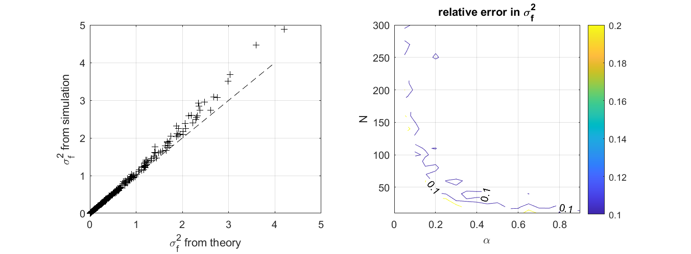
Figure 1: Variance for a single epoch from Monte-Carlo simulations, compared with the derived formula in Eq. (50), in the left panel, and the relative error (absolute value) in the right panel. The contour where the relative error is $0.1$ is indicated.

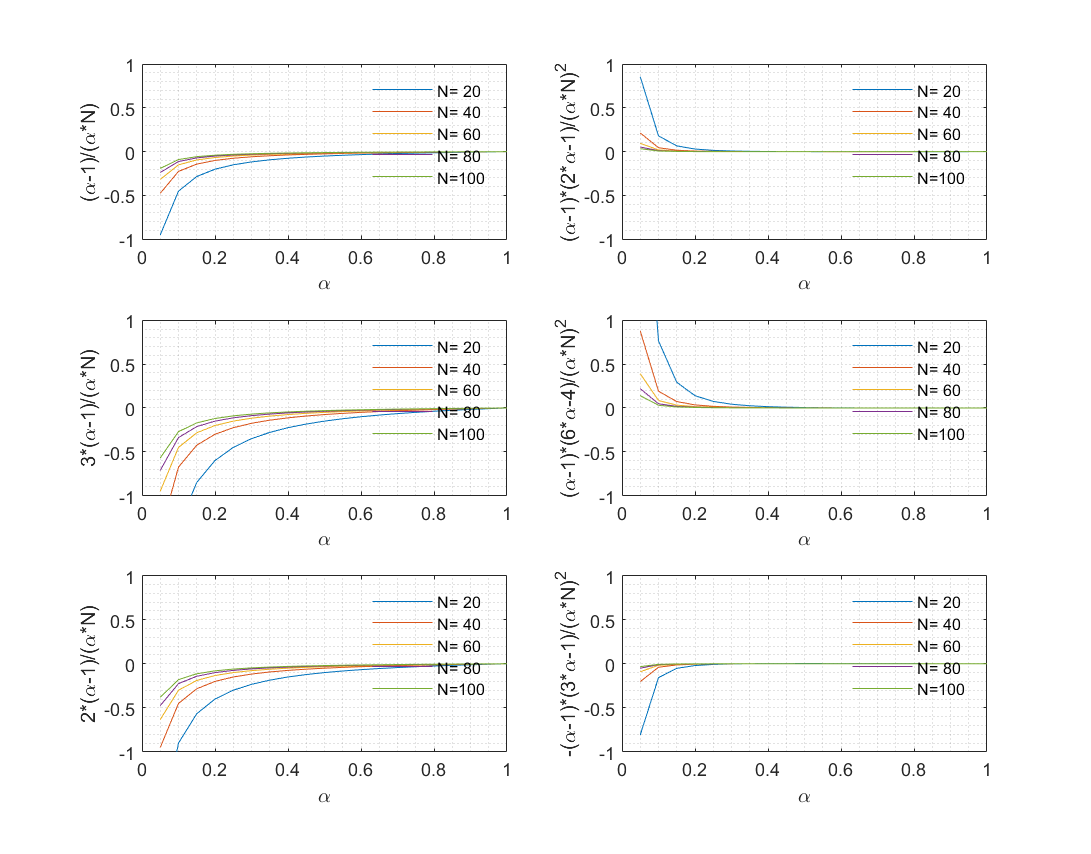
Figure 2: First two correction terms in the coefficients of $\sum_{i}\boldsymbol{\mathbf{E}}r_{i}^{2}$ (top panels), $\sum_{j\neq i}\boldsymbol{\mathbf{E}}r_{i}r_{j}$ (middle panels), and $\left\{\frac{1}{N}\sum_{i=1}^{N}\boldsymbol{\mathbf{E}}r_{i}\right\}^{2}$ (bottom panels), as functions of $\alpha$ and $N$, from Eq. (42). Since these are corrections to the coefficient of $1$, they are generally small for large $\alpha$ or $N.$

5 Discussion

Deriving convergent estimators for the variance of a spatial mean has broad relevance in the geosciences. These variance estimators depend only on the first and second moments of the physical field, and their convergence requires these to be finite. Many geophysical problems experience finite first and second moments, so convergent variance estimators can be derived for a broad range of settings, from hydrology to climate science. Convergence is furthermore assured if the probability of reporting individual observations is sufficiently large (i.e., $\alpha>1/2)$. We have illustrated this convergence by describing the behavior of successive terms in the series expansion for variance. The results indicate how we can get good estimators of the variance even with small datasets, as long as the probability of missing data is not too large. Alternately, if the chance of reporting an observation is small, the dataset had better be large (i.e., large $N$).

An important special case occurs if the weights are all uniform, as when arithmetic averages of the population are sought. This is sampling without replacement from the population of potential observation sites to make inferences about the properties of spatial averages. As in the present study, if the probability of individual sites being observed is held fixed, the total number of reported observations varies and follows the Binomial distribution. While this differs from the Bootstrap (Diaconis and Efron (1983)) in its design and in sampling without replacement, it still gives rise to useful nonparametric formulas of estimators that arise in analogous contexts (Hankin et al. (2019)), and involving statistics of subsamples from a population. Since the underlying theory is nonparametric and holds general lessons, further investigations of this situation is useful even though the exact formulation is different from the more typical treatments.

In the second part of this paper, we undertook a detailed analysis of this situation. Compared to the general problem, this special case with uniform weights inherits additional structure from our assumption of the independence of the $s_{i}$’s. As a consequence the moments in this case can be estimated directly through combinatorics. In particular, all coefficients of the moments appearing in the estimators can be easily computed via Stirling numbers of the second kind that count the number of distinct set partitions (Aigner (2007)). The problem of convergence of the approximate estimators is also made explicit as a result. Extending the analysis to higher approximations of the variance might be useful.

References

- Aigner (2007) Aigner, M. (2007), A Course in Enumeration, Springer.
- Bromwich and MacRobert (1991) Bromwich, T. J. I., and T. M. MacRobert (1991), An Introduction to the Theory of Infinite Series, New York: Chelsea.
- Diaconis and Efron (1983) Diaconis, P., and B. Efron (1983), Computer-intensive methods in statistics, Scientific American, 248, 116–131, doi:https://www.jstor.org/stable/24968902.
- Gandin (1993) Gandin, L. S. (1993), Optimal averaging of meteorological fields, US Department of Commerce Office Note 397.
- Gemignani (1970) Gemignani, M. C. (1970), Calculus and Statistics, Dover.
- Goodman and Hartley (1958) Goodman, L. A., and H. O. Hartley (1958), The Precision of Unbiased Ratio-Type Estimators, Journal of the American Statistical Association, 53, 491–508, doi:10.1080/01621459.1958.10501454.
- Hankin et al. (2019) Hankin, D. G., M. S. Mohr, and K. B. Newman (2019), Sampling Theory: For the Ecological and Natural Resource Sciences, Oxford University Press.
- Hartley and Ross (1954) Hartley, H. O., and A. Ross (1954), Unbiased ratio estimators, Nature, 174, 270–271, doi:10.1038/174270a0.
- Hinkley (1969) Hinkley, D. V. (1969), On the ratio of two correlated normal random variables, Biometrika, 56, 635–639, doi:10.1093/biomet/56.3.635.
- Hlawitschka (1994) Hlawitschka, W. (1994), The Empirical Nature of Taylor-Series Approximations to Expected Utility, The American Economic Review, 84, 713–719, doi:https://www.jstor.org/stable/2118079.
- Kagan (1997) Kagan, R. L. (1997), Averaging of Meteorological Fields, Kluwer Academic Publishers.
- Kendall et al. (1994) Kendall, M. G., A. Stuart, J. Forster, K. Ord, S. F. Arnold, and A. O’Hagan (1994), Kendall’s Advanced Theory of Statistics, Wiley.
- Kundu and Siddani (2007) Kundu, P. K., and R. K. Siddani (2007), A new class of probability distributions for describing the spatial statistics of area-averaged rainfall, Journal of Geophysical Research: Atmospheres, 112, 1–18, doi:10.1029/2006JD008042.
- Loistl (1976) Loistl, O. (1976), The Erroneous Approximation of Expected Utility by Means of a Taylor’s Series Expansion: Analytic and Computational Results, The American Economic Review, 66, 904–910, doi:https://www.jstor.org/stable/1827501.
- Markowitz (2015) Markowitz, H. (2015), Mean-variance approximations to expected utility, European Journal of Operations Research, 234, 346–355, doi:10.1016/j.ejor.2012.08.023.
- Morrissey et al. (1999) Morrissey, M. L., J. A. Maliekal, J. S. Greene, and J. Wang (1999), The uncertainty of simple spatial averages using rain gauge networks, Water Resources Research, 31, 2011–2017, doi:10.1029/95WR01232.
- Oehlert (1992) Oehlert, G. W. (1992), A note on the delta method, The American Statistician, 46, 27–29, doi:10.2307/2684406.
- Prakash et al. (2019) Prakash, S., A. K. Seshadri, J. Srinivasan, and D. S. Pai (2019), A new parameter to assess impact of rain gauge density on error in the estimate of monthly rainfall over India, Journal of Hydrometeorology, 20, 821–832, doi:10.1175/JHM-D-18-0161.1.
- Rodríguez-Iturbe and Mejía (1974) Rodríguez-Iturbe, I., and J. M. Mejía (1974), The design of rainfall networks in time and space, Water Resources Research, 10, 713–728, doi:10.1029/WR010i004p00713.
- Rudin (1976) Rudin, W. (1976), Principles of Mathematical Analysis, McGraw Hill.
- Seshadri (2018) Seshadri, A. K. (2018), Statistics of spatial averages and optimal averaging in the presence of missing data, Spatial Statistics, 25, 1–21, doi:10.1016/j.spasta.2018.04.002.
- Shen et al. (1994) Shen, S. S. P., G. R. North, and K.-Y. Kim (1994), Spectral approach to optimal estimation of the global average temperature, Journal of Climate, 7, 1999–2007, doi:10.1175/1520-0442(1994)007<1999:SATOEO>2.0.CO;2.
- Vershynin (2018) Vershynin, R. (2018), High Dimensional Probability: An Introduction with Applications in Data Science, Cambridge University Press.
- Villarini et al. (2008) Villarini, G., P. V. Mandapaka, W. F. Krajewski, and R. J. Moore (2008), Rainfall and sampling uncertainties: A rain gauge perspective, Journal of Geophysical Research: Atmospheres, 113, 1–12, doi:10.1029/2007JD009214.
- Vinnikov et al. (2004) Vinnikov, K. Y., A. Robock, N. C. Grody, and A. Basist (2004), Analysis of diurnal and seasonal cycles and trends in climatic records with arbitrary observation times, Geophysical Research Letters, 31, 1–5, doi:10.1029/2003GL019196.
- Weir (1973) Weir, A. J. (1973), Lebesgue Integration and Measure, Cambridge University Press.