Thermodynamic crossovers in supercritical fluids

Abstract

Can liquid-like and gas-like states be distinguished beyond the critical point, where the liquid-gas phase transition no longer exists and conventionally only a single supercritical fluid phase is defined? Recent experiments and simulations report strong evidence of dynamical crossovers above the critical temperature and pressure [1, 2, 3]. Despite using different criteria, existing theoretical explanations generally consider a single crossover line separating liquid-like and gas-like states in the supercritical fluid phase [4, 5, 6, 7, 8, 9, 10]. We argue that such a single-line scenario is inconsistent with the supercritical behavior of the Ising model, which has two crossover lines due to its symmetry, violating the universality principle of critical phenomena. To reconcile the inconsistency, we define two thermodynamic crossover lines in supercritical fluids as boundaries of liquid-like, indistinguishable and gas-like states. Near the critical point, the two crossover lines follow critical scalings with exponents of the Ising universality class, supported by calculations of theoretical models and analyses of experimental data from the standard database [11]. The upper line agrees with crossovers independently estimated from the inelastic X-ray scattering data of supercritical argon [1, 2], and from the small-angle neutron scattering data of supercritical carbon dioxide [3]. The lower line is verified by the equation of states for the compressibility factor. This work provides a fundamental framework for understanding supercritical physics in general phase transitions.

According to textbook knowledge, no liquid-gas phase transitions exist in the supercritical fluid state of matter. Then, how does a liquid transform into a gas (or vice versa) along a path by passing the critical point? Many studies propose that there should be a line of supercritical crossovers between liquid-like and gas-like states. Such a crossover line divides the phase diagram above the critical point into regimes with different physical properties, which can be connected without going through any thermodynamic singularity. The following supercritical crossover lines have been defined.

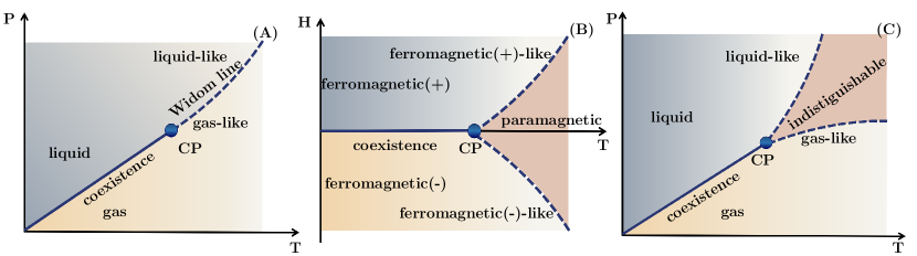
Figure 1: Schematic phase diagrams. (A) Liquid-gas (pressure $P$ vs temperature $T$ ) phase diagram with a Widom line (dashed) separating liquid-like and gas-like regimes above the critical point (CP). (B) Phase diagram of the Ising model, with two supercritical crossover lines (dashed) separating positive ferromagnetic-like, paramagnetic, and negative ferromagnetic-like regimes. (C) Liquid-gas phase diagram with two supercritical crossover lines (dashed), $L^{\pm}$, separating liquid-like, indistinguishable, and gas-like regimes.

(I) Widom line [12, 4, 13, 14, 15, 16, 17, 18, 19, 20, 21] (see Fig. 1A), defined as the line of maxima in thermodynamic response functions (e.g., specific heat or compressibility) under the fixed pressure $P$ (or temperature $T$) condition. The maximum value  increases approaching the critical point, and diverges at the point. The lines of maxima determined according to different response functions are assumed to converge into a single line near the critical point, which emanates from the critical point.

(II) Fisher-Widom line [5, 22, 23, 24, 25, 26, 27], defined as the boundary between states with exponential (gas-like) and oscillatory (liquid-like) long-range decays of the pair correlation function. Liquid-like and gas-like states are distinguished based on the structure of configuration, i.e., the spatial distribution of particles.

(III) Frenkel line [6, 28, 29, 30, 31, 32, 33, 34, 35, 36, 37], which separates liquid-like and gas-like states based on whether viscoelastic dynamics are present. Within the vibrational time, liquids behave like amorphous solids – particles vibrate around their equilibrium positions; beyond the structural relaxation time (diffusion time), particles diffuse, and the equilibrium configuration decorrelates from the initial one. As $T$ increases (or $P$ decreases), this liquid-like picture breaks down at the Frenkel line, where the vibration time becomes comparable with the structural relaxation time, and the system turns into a gas-like state.

(IV) Nishikawa line [7, 38, 39], defined by the “ridge” of the density fluctuation profile on the $P$-$T$ phase diagram, where the density fluctuation maximizes.

(V) Symmetry line [8], defined at the zero skewness in the particle number distribution for the grand canonical ensemble. Liquid-like behavior is characterized by a negative skewness indicating the favor of particle deletion, whereas gas-like behavior is characterized by a positive skewness indicating the favor of particle insertion.

(VI) Percolation lines [9, 40], determined by the loci of the percolation transition of available volume accessible to any single mobile atom, and that of the cluster formed by bonded atoms. The percolation line of the hydrogen bond network has also been studied in supercritical water [10], but the method cannot be applied to supercritical fluids without hydrogen bonds.

The above proposals are theoretically inconsistent with the supercritical crossover lines of the Ising model (see Fig. 1B). To show that, let us first discuss the analogies between the two systems, and the supercritical behavior of the Ising model.

The liquid-gas critical point and the magnetic phase transition in a three-dimensional (3D) Ising model belong to the same $O(1)$ universality class [41, 42]. According to the principle of universality in statistical mechanics, they should display critical scalings with the same exponents. The pressure $P$ and susceptibility $\kappa_{T}\equiv\frac{P_{\rm c}}{\rho_{\rm c}}\left(\frac{\partial\rho}{\partial P}\right)_{T}$ (or the compressibility $\beta_{T}=\frac{1}{\rho}\left(\frac{\partial\rho}{\partial P}\right)_{T}$) in the former are analogous of the magnetic field $H$ and magnetic susceptibility $\chi=\left(\frac{\partial m}{\partial H}\right)_{T}$ in the latter, where $P_{\rm c}$ and $\rho_{\rm c}$ are the critical pressure and density. Here $P$ and $H$ play the role of external fields; $\kappa_{T}$ and $\chi$ characterize the response of the order parameter (i.e., the liquid-gas density difference $\delta\rho$ and the magnetization $m$ respectively) to the external field. Following the definition of Widom line, it is immediately apparent that in the Ising model, the maxima of $\chi$ at constant $H$ form two crossover lines (denoted by $L^{+}$ and $L^{-}$) above the critical temperature $T_{\rm c}$. Due to the $Z_{2}$ symmetry of the Ising model, the two lines $L^{\pm}$ are perfectly symmetric with respect to the coexistence line $H=0$. Along $L^{\pm}$ lines, the field and order parameter follow critical scalings,

$$|H^{\pm}|\sim(T-T_{\rm c})^{\beta+\gamma},$$ (1)

and

$$|m^{\pm}|\sim(T-T_{\rm c})^{\beta},$$ (2)

established by analytic calculations of the mean-field model and Monte-Carlo numerical simulations of 2D and 3D models (see Supplementary Information SI Sec. S1), where $\beta$ and $\gamma$ are universal critical exponents (for the 3D Ising universality class, $\beta\simeq 0.3265$ and $\gamma\simeq 1.237$ [43]).

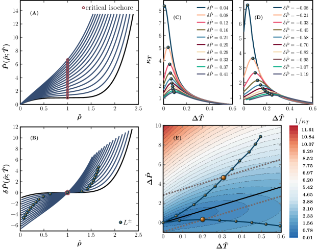
Figure 2: Determination of supercritical crossover lines $L^{\pm}$ in argon. (A) Isothermal EOSs, $\hat{P}(\hat{\rho};\hat{T})$, for $\hat{T}=1.00,1.07,1.13,1.20,1.27,1.33,1.40,1.46,1.53,1.60,1.66,1.73,1.80,1.86,1.93$. (from bottom to top). (B) Shifted EOSs $\delta\hat{P}(\hat{\rho};\hat{T})$. (C-D) Susceptibility $\kappa_{T}$ as a function of $\Delta\hat{T}$, for a few fixed $\delta\hat{P}$. The loci of peaks determine (C) $L^{+}$ and (D) $L^{-}$ lines, for $\delta\hat{P}>0$ and $\delta\hat{P}<0$ respectively. (E) The color map of $1/\kappa_{T}$ in the $\Delta\hat{P}-\Delta\hat{T}$ diagram, with constant $1/\kappa_{T}$ contour lines (solid thin lines). As an example, we show two parallel paths (dashed brown lines) to the critical isochore (think black line). Such a parallel path has a point of tangency (big orange ball) with a certain constant $1/\kappa_{T}$ contour; along this parallel path, the point of tangency corresponds to the maximum of $\kappa_{T}$ as defined in $L^{\pm}$. In panels (B-E), the $L^{\pm}$ lines are represented by the same symbol.

The $L^{\pm}$ lines in the Ising model have the following properties. (i) They separate three states, positive ferromagnetic-like, paramagnetic and negative ferromagnetic-like states (see Fig. 1B). The two lines do not merge to a common line even in the vicinity of the critical point – they coincide precisely at the critical point. (ii) Both lines emanate from the critical point, and (iii) follow the critical scalings Eqs. (1) and (2). None of the above-mentioned supercritical crossover lines (I-VI) simultaneously satisfy all these three properties (see SI Table S1 for a summary). Definitions (I-V) give one single crossover line; definition (VI) gives two percolation lines, but they do not emanate from the critical point. The (II) Fisher-Widom line, (III) Frenkel line, and (VI) percolation lines do not pass through the critical point, and thus are without any critical scaling. The (I) Widom line, (IV) Nishikawa line and (V) symmetry line, although emanating from the critical point, do not satisfy the critical scalings Eqs. (1) and (2). In short, even though it is well established that liquid-gas and ferromagnetic-paramagnetic critical points belong to the same 3D Ising universality class, their supercritical physics is not yet unified within the framework of critical universality.

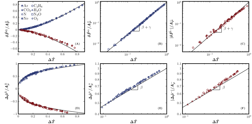
Figure 3: Scalings of supercritical crossover lines $L^{\pm}$ near the critical point in eight substances. (A) $\delta\hat{P}^{\pm}/A_{P}^{\pm}$ as a function of $\Delta\hat{T}$. The data points are fitted to $|\delta\hat{P}^{\pm}|=A_{P}^{\pm}\Delta\hat{T}^{\beta+\gamma}$ (solid lines), where $A_{P}^{\pm}$ are non-universal fitting parameters (see SI Table S2 for values of $A_{P}^{\pm}$), and the exponents are fixed by the 3D Ising universality values, $\beta=0.3265$ and $\gamma=1.237$. (B) and (C) are log-log plots for $L^{+}$ and $L^{-}$ respectively. (D-F) Similar plots for the scaling $|\Delta\hat{\rho}^{\pm}|=A_{\rho}^{\pm}\Delta\hat{T}^{\beta}$.

To resolve the inconsistency, we propose a new definition of the crossover lines in supercritical fluids (see Fig. 1C). The method is explained in Fig. 2, taking argon as an example. The general procedure is as follows. (i) The experimental data of supercritical isothermal equations of states (EOSs), $\hat{P}(\hat{\rho};\hat{T})$, are collected from the National Institute of Standards and Technology (NIST) database [11] and plotted in Fig. 2(A), where the state variables are rescaled by their critical values, $\hat{T}=T/T_{\rm c}$, $\hat{P}=P/P_{\rm c}$ and $\hat{\rho}=\rho/\rho_{\rm c}$. (ii) The critical isochore $\hat{P}(\hat{\rho}=1;\hat{T})$ is subtracted from the original EOSs, giving the shifted EOSs (Fig. 2B), $\delta\hat{P}(\hat{\rho};\hat{T})=\hat{P}(\hat{\rho};\hat{T})-\hat{P}(1;\hat{T})$. Here the critical isochore is analogous to the $H=0$ line in the Ising model; in particular, along the critical isochore, $\kappa_{T}$ exhibits the standard critical scaling, $\kappa_{T}\sim(T-T_{\rm c})^{-\gamma}$, for $T>T_{\rm c}$. Thus the critical isochore above the critical point can be considered as an extension of the coexistence line. Due to this symmetry, we take the critical isochore as the reference line to obtain shifted EOSs. Similar to the isothermal EOSs $H(m;T)$ of the Ising model, which all intersect at a point $(m=0,H=0)$, the shifted EOSs $\delta\hat{P}(\hat{\rho};\hat{T})$ intersect at a common point $(\hat{\rho}=0,\delta\hat{P}=0)$. The susceptibility $\kappa_{T}$ is the inverse slope of the shifted EOS for constant $\hat{T}$. (iii) For a fixed $\delta\hat{P}$, the compressibility $\kappa_{T}(\hat{T};\delta\hat{P})$ peaks at $\hat{T}_{\rm max}^{+}(\delta\hat{P})$ for $\delta\hat{P}>0$ (see Fig. 2C) and $\hat{T}_{\rm max}^{-}(\delta\hat{P})$ for $\delta\hat{P}<0$ (see Fig. 2D). Connecting the points $\hat{T}_{\rm max}^{\pm}(\delta\hat{P})$ together gives the two lines $L^{\pm}$ (see Fig. 2B). Figure 2E shows $L^{\pm}$ lines in the $\Delta\hat{P}-\Delta\hat{T}$ phase diagram, where $\Delta\hat{P}=P/P_{\rm c}-1$ and $\Delta\hat{T}=T/T_{\rm c}-1$. These two lines separate liquid-like, liquid-gas-indistinguishable and gas-like phases, which are counterparts of positive ferromagnetic-like, paramagnetic and negative ferromagnetic-like phases in the Ising model. The described procedure applies generally to the van der Waals EOS, a standard theoretical model for gases and liquids (see SI Sec. S3), and to the experimental EOSs of other substances (e.g., water, see SI Sec. S4).

It is clear that $L^{\pm}$ lines are defined according to thermodynamics rather than dynamics. The criterion of $L^{\pm}$ is similar to that of the Widom line; the key difference is that the maxima of the response function $\kappa_{T}$ are evaluated along paths parallel to the critical isochore (see Fig. 2E), instead of along constant-pressure or constant-temperature paths. Each parallel path that is $\delta\hat{P}$ away from the critical isochore is tangential to a constant-$\kappa_{T}$ contour line, at the point of tangency $\hat{T}_{\rm max}^{+}(\delta\hat{P})$ or $\hat{T}_{\rm max}^{-}(\delta\hat{P})$. Note that for better visualization, in Fig. 2E we plot the color map and contour lines of constant $1/\kappa_{T}$, where a maximum becomes a minimum without changing its location.

Using a linear scaling theory (see SI Sec. S5) [17], we establish theoretically the scalings of $L^{\pm}$ lines near the liquid-gas critical point,

$$|\delta\hat{P}^{\pm}|\sim(T-T_{\rm c})^{\beta+\gamma},$$ (3)

and

$$|\Delta\hat{\rho}^{\pm}|\sim(T-T_{\rm c})^{\beta},$$ (4)

where $\delta\hat{P}^{\pm}$ and $\Delta\hat{\rho}^{\pm}$ are values on the $L^{\pm}$ lines ($\Delta\hat{\rho}=\rho/\rho_{\rm c}-1$). To verify Eqs. (3) and (4), we collect the experimental data of eight common substances, including water ($\rm{H_{2}O}$), carbon dioxide ($\rm{CO_{2}}$), argon ($\rm{Ar}$), nitrogen ($\rm{N}$), neon ($\rm{Ne}$), propane ($\rm{C_{3}H_{8}}$), dinitrogen monoxide ($\rm{N_{2}O}$) and oxygen ($\rm{O_{2}}$) from the NIST database, and evaluate their $L^{\pm}$ lines using the same approach as demonstrated above for argon (Fig. 2). Figure 3 shows that both scalings are confirmed by the data of all eight substances examined, with the 3D Ising universality class exponents. Furthermore, the scalings Eqs. (3) and (4) are robust, independent of which thermodynamic response function is chosen to determine the maxima (see SI Sec. S5 and S7). Equations (1-4) recover the critical universality: the two supercritical crossover lines $L^{\pm}$ obey scaling laws with the same exponents in both liquid-gas and Ising systems.

Next we compare $L^{\pm}$ lines with supercritical crossovers reported previously in two sets of independent experiments (simulations) [1, 2, 3]. In the first set, dynamical supercritical crossovers are estimated based on the sound dispersion data obtained for supercritical argon, by inelastic X-ray scattering experiments and molecular dynamics simulations [1, 2]. From these data, sharp crossovers are determined between a regime of positive sound dispersion ratio that increases with $\rho$ at constant $T$, and a regime of weak, $\rho$-independent sound dispersion (see SI Sec. S8). The increasing positive dispersion in the first regime reflects typical viscoelastic behavior of liquid-like states, implying the existence of two relaxation mechanisms – structural relaxations related to the so-called $\alpha$-processes and microscopic relaxations related to nearest-neighbour interactions [1, 44, 45]. In the second regime, the weak constant dispersion implies that the structural relaxations disappear and only the microscopic relaxations remain, representing non-liquid-like (gas-like or indistinguishable) states [46, 47]. In Fig. 4(A), the dynamical crossovers from sound-dispersion data are compared with $L^{\pm}$ lines and previously proposed crossover lines (I-VI). The best agreement is found between the experimental dynamical crossovers and the $L^{+}$ line.

In the second experiment, a supercritical crossover is estimated based on the small-angle neutron scattering data of carbon dioxide [3]. The data show that, above a crossover pressure, $\hat{P}_{\rm cro}=1.63$ ($P_{\rm cro}=120$ bar) at a fixed $\hat{T}=1.046$ ($T=45^{\circ}$ C), the density and density fluctuation are enhanced compared with the standard NIST data for a homogeneous state. It is expected that the formation of liquid droplets causes such enhancement; correspondingly $\hat{P}_{\rm cro}$ indicates a crossover to liquid-like behavior. The location of this crossover point is consistent with $L^{+}$ line, as shown in Fig. 4(B).

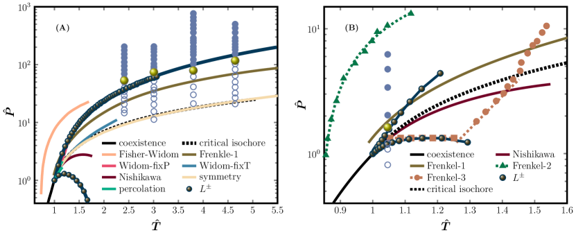
Figure 4: Comparison between supercritical crossover lines and experimental (simulation) data. (A) $\hat{P}$-$\hat{T}$ diagram of supercritical argon. The data points of $L^{\pm}$ lines are obtained in Fig. 2, and fitted to the scaling form Eq. (3) (solid lines, see SI Sec. S7 for a discussion on the fitting). Filled and open blue circles are data points collected from  [1, 2] at four different $\hat{T}$: the filled circles are with positive increasing sound dispersion, and the open circles are with weak constant sound dispersion; they are separated by crossover points indicated by yellow balls (see SI Sec. S8). The Fisher-Widom line  [48], the Frenkle line for a Lennard Jones fluid [6] (Frenkel-1), the symmetry line [8] and percolation lines [9] are copied from the cited publications correspondingly. The Nishikawa line is evaluated in SI Sec. S10 according to its definition. The Widom lines are determined based on the NIST EOSs, for fixed $P$ and fixed $T$. An enlarged view near the critical point is provided in Fig. S15. (B) $\hat{P}$-$\hat{T}$ diagram of supercritical carbon dioxide. Filled and open blue circles are data points collected from  [3]: the filled/open circles are with/without enhanced density fluctuations compared to the NIST data, separated by the crossover point (yellow ball). The Frenkel line depends on the criterion used: in addition to Frenkel-1, two more Frenkel lines are plotted, Frenkel-2 from [49] and Frenkel-3 from [50, 3]. The Nishikawa line is from [51].

The above two examples demonstrate remarkable coincidences between the $L^{+}$ line and previous experimental results. The prediction of $L^{-}$ line remains to be examined in future experiments. In SI Sec. S11, we show that the $L^{-}$ line can be validated independently by the behavior of EOS for the compressibility factor above the critical temperature. However, we expect that the differences between liquid-like and indistinguishable states might be subtle to detect directly in experiments. Finally, it should be straightforward to generalize the present analysis to other phase transitions, including liquid-liquid phase transitions [4], quantum phase transitions [52], non-equilibrium phase transitions such as liquid-glass transitions [53], and phase transitions in dusty plasmas [54].

Supplementary Information

S1 Ising model

The Hamiltonian of the Ising model is [55],

$$\mathcal{H}=-J\displaystyle\sum_{\left<i,j\right>}s_{i}s_{j}-H\sum_{i=1}^{N}s_{i},$$ (S1)

where $J$ is a coupling constant, $s_{i}=\pm 1$ the value of spin on the $i$-th site, $N$ the total number of spins, $H$ the external magnetic field, and $\left<i,j\right>$ stands for nearest-neighbor spin pairs. The model is defined on a square lattice in $d$ dimensions. The mean magnetization is $m=\frac{1}{N}\left\langle\sum_{i=1}^{N}s_{i}\right\rangle$, where $\left\langle\ldots\right\rangle$ is the ensemble average, and the susceptibility is $\chi=\left(\frac{\partial m}{\partial H}\right)_{T}$.

According to the definition, on the supercritical ($T>T_{\rm c}$) crossover lines $L^{\pm}$, $\chi$ is maximum, i.e.,

$$\left(\frac{\partial\chi}{\partial T}\right)_{H}=0,$$ (S2)

where $T_{\rm c}$ is the critical temperature. The purpose of this section is to show that on $L^{\pm}$ the order parameter $m^{\pm}$ and the field $H^{\pm}$ satisfy two scalings, Eqs. (1) and (2), near the critical point. We first derive these two scalings analytically from a mean-field calculation, and then demonstrate that they also hold in two and three dimensions ($d=2$ and 3) using Monte Carlo simulations.

S1.1 Mean-field theory

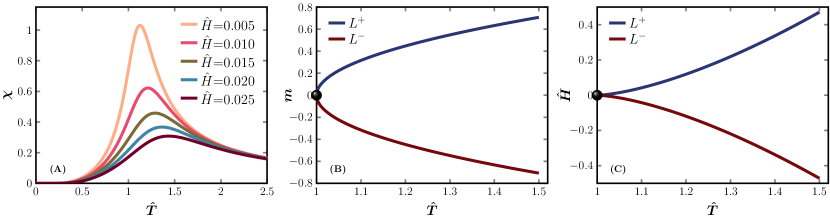
Figure S1: Supercritical crossover lines $L^{\pm}$ in the mean-field Ising model. (A) Magnetic susceptibility $\chi$ as a function of the reduced temperature $\hat{T}$, for a few different reduced magnetic fields $\hat{H}$. The peaks determine the supercritical crossover lines $L^{\pm}$. Along $L^{\pm}$, (B) $m^{\pm}$ changes with $\hat{T}$ following Eq. (S8), and (C) $\hat{H}^{\pm}$ changes with $\hat{T}$ following Eqs. (S9).

With the mean-field approximation, $m$ and $\chi$ are easy to calculate [56]:

$$m=\tanh{\left[\beta(H+qJm)\right]},$$ (S3)

and

$$\chi=\frac{\beta}{\cosh^{2}{\left[\beta(H+qJm)\right]-\beta Jq}},$$ (S4)

where $q=2d$ is the coordination number (i.e., the number of nearest neighbors of each spin), and $\beta=1/{k_{\rm B}T}$ the inverse temperature. We set the Boltzmann constant $k_{\rm B}=1$.

In the following derivations, we switch to the reduced parameters $\hat{H}=H/T_{\rm c}$ and $\hat{T}=T/T_{\rm c}$, where $T_{\rm c}=qJ$. With the reduced parameters, Eq. (S3) becomes,

$$\begin{aligned} m&=\tanh{\left[\frac{(\hat{H}+m)}{\hat{T}}\right]}\\ &\approx\frac{\hat{H}+m}{\hat{T}}-\frac{1}{3}\left(\frac{\hat{H}+m}{\hat{T}}\right)^{3},\end{aligned}$$ (S5)

where we have expanded it up to the third order, assuming that $\hat{H}$ and $m$ are small near the critical point. Defining $\hat{\chi}=T_{\rm c}\chi$, from Eq. (S5) we obtain,

$$\begin{aligned} \hat{\chi}=\left(\frac{\partial{m}}{\partial{\hat{H}}}\right)_{\hat{T}}=\frac{1-(\hat{H}+m)^{2}/\hat{T}^{2}}{\hat{T}-1+(\hat{H}+m)^{2}/\hat{T}^{2}}.\end{aligned}$$ (S6)

Making a change of variable $A=(\hat{H}+m)/\hat{T}$, and taking the partial derivative of Eq. (S6) with respect to the temperature, we get

$$\begin{aligned} \left(\frac{\partial\hat{\chi}}{\partial\hat{T}}\right)_{\hat{H}}=\frac{(3A^{2}-1)(\hat{T}-1+A^{2})+2A^{2}(1-A^{2})}{(\hat{T}-1+A^{2})^{3}},\end{aligned}$$ (S7)

which should be $0$ on the $L^{\pm}$. The solution of $\left(\frac{\partial\hat{\chi}}{\partial\hat{T}}\right)_{\hat{H}}=0$ is, $(A^{\pm})^{2}=\hat{T}-1$, or,

$$\left|m^{\pm}\right|=\left(\hat{T}-1\right)^{1/2},$$ (S8)

near the critical point, where the exponent is equal to the mean-field exponent $\beta=1/2$ (note that $\left|\hat{H}^{\pm}\right|$ is higher order; see Eq. S9). Equation (S8) gives the scaling relationship between the order parameter and temperature on $L^{\pm}$ (see Fig. S1). Using Eq. (S5), we can convert Eq. (S8) into a relationship between the external field $\hat{H}^{\pm}$ and $\hat{T}$ on $L^{\pm}$,

$$\left|\hat{H}^{\pm}\right|=\frac{4}{3}\left(\hat{T}-1\right)^{3/2},$$ (S9)

where the exponent is equal to $\beta+\gamma=3/2$ with the mean-field exponents $\beta=1/2$ and $\gamma=1$. The mean-field scalings are plotted in Fig. S1.

Equations (S8) and (S9) are the mean-field form of scalings Eqs. (1) and (2). In Sec. S5, we will derive these scalings using a general linear scaling theory without the mean-field approximation.

S1.2 Monte Carlo simulations in two and three dimensions

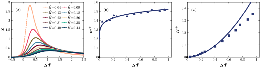
Figure S2: Supercritical crossover lines $L^{\pm}$ in the 2D Ising model. Results are obtained from Monte Carlo simulations. (A) Magnetic susceptibility $\chi$ as a function of the reduced temperature $\hat{T}$, for a few different reduced magnetic fields $\hat{H}$. The peaks determine the supercritical crossover line $L^{+}$ (the $L^{-}$ line is symmetric to the $L^{+}$ line and not shown). (B) The magnetization $m^{+}$ and (C) reduced field $\hat{H}^{+}$ along the $L^{+}$ line are plotted as functions of $\Delta\hat{T}$. The lines represent fits, $m^{+}=A_{m}\Delta\hat{T}^{\beta}$ and $\hat{H}^{+}=A_{H}\Delta\hat{T}^{\beta+\gamma}$, where $A_{m}=0.523$ and $A_{H}=0.521$ are fitting parameters (see Fig. S3 for corresponding log-log plots).

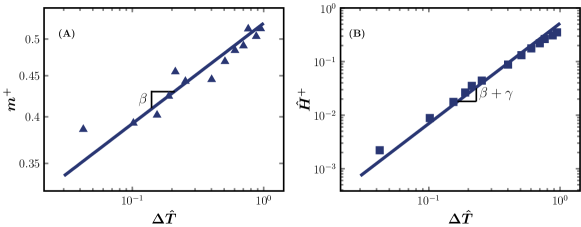
Figure S3: Scaling laws of the $L^{+}$ line in the 2D Ising model. (A) The magnetization $m^{+}$ and (B) reduced field $\hat{H}^{+}$ as functions of $\Delta\hat{T}$, in log-log scales. The lines represent fits, $m^{+}=A_{m}\Delta\hat{T}^{\beta}$ and $\hat{H}^{+}=A_{H}\Delta\hat{T}^{\beta+\gamma}$, where $A_{m}=0.523$ and $A_{H}=0.521$ are fitting parameters.

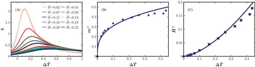
Figure S4: Supercritical crossover lines $L^{\pm}$ in the 3D Ising model. Results are obtained from Monte Carlo simulations. (A) Magnetic susceptibility $\chi$ as a function of the reduced temperature $\hat{T}$ (for this panel the lattice size is $12\times 12\times 12$), for a few different reduced magnetic fields $\hat{H}$. The peaks determine the supercritical crossover line $L^{+}$. (B) The magnetization $m^{+}$ and (C) reduced field $\hat{H}^{+}$ along the $L^{+}$ line are plotted as functions of $\Delta\hat{T}$. The lines represent fits, $m^{+}=A_{m}\Delta\hat{T}^{\beta}$ and $\hat{H}^{+}=A_{H}\Delta\hat{T}^{\beta+\gamma}$, where $A_{m}=0.652$ and $A_{H}=0.719$ are fitting parameters (see Fig. S5 for corresponding log-log plots).

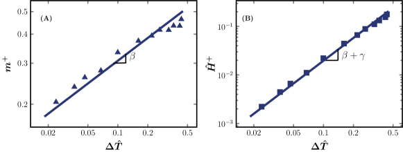
Figure S5: Scaling laws of the $L^{+}$ line in the 3D Ising model. (A) The magnetization $m^{+}$ and (B) reduced field $\hat{H}^{+}$ as functions of $\Delta\hat{T}$, in log-log scales. The lines represent fits, $m^{+}=A_{m}\Delta\hat{T}^{\beta}$ and $\hat{H}^{+}=A_{H}\Delta\hat{T}^{\beta+\gamma}$, where $A_{m}=0.652$ and $A_{H}=0.719$ are fitting parameters.

We study the Ising model in both two (2D) and three (3D) dimensions to validate the scaling relationships Eqs. (1) and (2), using Monte Carlo simulations with the wolff algorithm [57, 58]. The lattice size is $40\times 40$ in 2D and $25\times 25\times 25$ in 3D. The mean magnetization is computed using the definition, $m=\frac{1}{N}\left\langle\sum_{i=1}^{N}s_{i}\right\rangle$, and the magnetic susceptibility is computed using,

$$\chi=\left(\frac{\partial m}{\partial H}\right)_{T}=\beta N\left(\left\langle m^{2}\right\rangle-{\left\langle m\right\rangle}^{2}\right).$$ (S10)

In simulations, $m$ and $\chi$ are obtained by averaging over $10^{4}$ independent equilibrium configurations. For a few given $\hat{H}$, the magnetic susceptibility $\chi$ is plotted as a function of temperature $\hat{T}$ in Fig. S2(A) and Fig. S4(A), from which the peaks are located. The supercritical crossover lines determined in this way can be well fitted to scalings Eqs. (1) and (2), as shown in Figs. S2-S5. In the fitting, the exponents are fixed to the known values: $\beta=1/8$, $\gamma=7/4$ in 2D [59], and $\beta=0.326$, $\gamma=1.237$ in 3D [43]; the prefactor is treated as a fitting parameter.

S2 Summary of supercritical crossover lines in the literature

Table S1 summarizes supercritical crossover lines existing in the literature, compared to the proposal of this study.

Table S1: Summary of crossover lines in supercritical fluids.

crossover lines	number of lines	emanating from the critical point?	obeying critical scalings Eq. (3) and (4)?
Widom line [4]	one	yes	no
Fisher-Widom line [5]	one	no	no
Frankel line [6]	one	no	no
Nishikawa line [7]	one	yes	no
symmetry line [8]	one	yes	no
percolation lines [9]	two	no	no
$L^{\pm}$ lines (this study)	two	yes	yes

S3 van der Waals equation of state

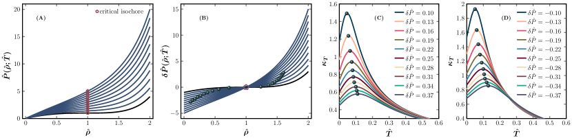
Figure S6: Determination of crossover lines $L^{\pm}$ of the van der Waals equation of state. (A) Isothermal EOSs, $\hat{P}(\hat{\rho};\hat{T})$, above the critical temperature. The black line is critical isotherm, and dark blue lines are other isotherms (from bottom to top, $\hat{T}=1.00,1.10,1.20,1.30,1.40,1.50,1.60,1.70,1.80,1.90,2.00.$). The critical isochore is marked by pentagons. (B) Shifted EOSs $\delta\hat{P}(\hat{\rho};\hat{T})$. The Susceptibility $\kappa_{T}=\left(\frac{\partial\hat{\rho}}{\partial\hat{P}}\right)_{\hat{T}}$ is plotted as a function of $\hat{T}$, for a few fixed (C) $\delta\hat{P}>0$ and (D) $\delta\hat{P}<0$; the loci of peaks determine $L^{+}$ and $L^{-}$ respectively (circles). The meanings of symbols are the same in all panels.

The van der Waals equation is one of the most widely used equation of state (EOS) for describing the liquid-gas phase transition. The reduced form of the van der Waals equation is,

$$\left(\hat{P}+\frac{3}{\hat{V}^{2}}\right)\left(3\hat{V}-1\right)=8\hat{T},$$ (S11)

where $\hat{P}=P/P_{\rm c}$, $\hat{V}=V/V_{\rm c}$ and $\hat{T}=T/T_{\rm c}$ are the reduced pressure, volume and temperature respectively, and $P_{\rm c}$, $V_{\rm c}$ and $T_{\rm c}$ are the pressure, volume and temperature of the critical point.

S3.1 Determination of $L^{\pm}$ lines

The supercritical crossover lines $L^{\pm}$ are obtained numerically following the procedure described below. A similar procedure is used to obtain $L^{\pm}$ of argon in the main text (see Fig. 2).

• Plot the isothermal EOSs $\hat{P}(\hat{\rho};\hat{T})$ above the critical temperature, where $\hat{\rho}=1/\hat{V}$ is the reduced density (see Fig. S6(A)).

• Subtract the critical isochore $\hat{P}(1;\hat{T})$ from the original EOS $\hat{P}(\hat{\rho};\hat{T})$. In the shifted EOSs, $\delta\hat{P}(\hat{\rho};\hat{T})=\hat{P}(\hat{\rho};\hat{T})-\hat{P}(1;\hat{T})$, the critical isochore line $\hat{P}(1;\hat{T})$ becomes a single point $\delta\hat{P}(1;\hat{T})=0$ that coincides with the critical point (see Fig. S6(B)). All shifted EOSs $\delta\hat{P}(\hat{\rho};\hat{T})$ intersect at this point.

• Along constant-$\delta\hat{P}$ paths, find the maxima of the susceptibility $\kappa_{T}=\left(\frac{\partial\hat{\rho}}{\partial(\delta\hat{P})}\right)_{\hat{T}}$, which give $L^{\pm}$ (see Fig. S6(C) and (D)). The constant-$\delta\hat{P}$ paths correspond to lines parallel to the the critical isochore in the $\hat{P}-\hat{T}$ phase diagram.

S3.2 $L^{\pm}$ lines in pressure-temperature and pressure-volume phase diagrams

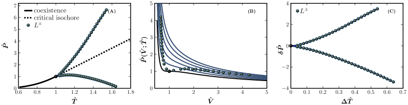
Figure S7: Crossover lines $L^{\pm}$ of the van der Waals equation of state. (A) Pressure-temperature ($\hat{P}-\hat{T}$) diagram. (B) Pressure-volume ($\hat{P}-\hat{V}$) diagram, where the lines are isotherms for $\hat{T}=1.00,1.10,1.20,1.30,1.40,1.50.$ (from bottom to top). (C) $\delta\hat{P}-\Delta\hat{T}$ diagram.

The above determined crossover lines $L^{\pm}$ are plotted in pressure-temperature ($\hat{P}-\hat{T}$) and pressure-volume ($\hat{P}-\hat{V}$) diagrams (see Fig.  S7(A) and Fig. S7(B)). In the $\delta\hat{P}-\Delta\hat{T}$ diagram, $L^{+}$ is nearly symmetric to $L^{-}$ (see Fig. S7(C)), similar to the case of Ising model (see Fig. S1A).

S4 $L^{\pm}$ lines of water

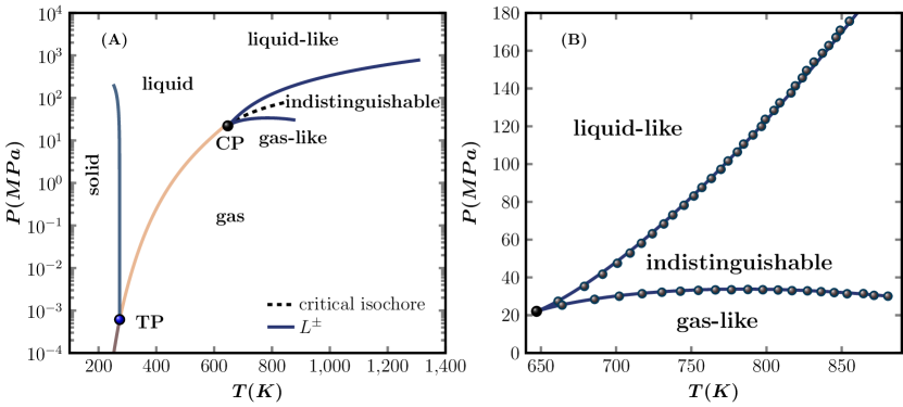
Figure S8: Supercritical crossover lines $L^{\pm}$ of water. (A) Pressure-temperature phase diagram of water. $L^{\pm}$ lines have been included in the diagram, separating liquid-like, indistinguishable and gas-like regimes. The triple point (TP) and critical point (CP) are also indicated. (B) $L^{\pm}$ lines in the vicinity of the critical point. Points are determined from the maximum of $\kappa_{T}$. Lines represent fitting to the data points, following the second fitting method explained in Sec. S7.1.

Crossovers lines of supercritical water have been investigated in many studies [48, 20, 19, 60, 61, 62, 10, 39, 36], using various definitions listed in Table S1. Figure S8(A) shows the phase diagram of water [63], where we have included thermodynamic crossover lines $L^{\pm}$. The original EOS data are collected from the NIST database [11], and $L^{\pm}$ are determined in the same way as for argon (see Fig. S8(B) for an enlarged view).

S5 Linear scaling theory

S5.1 Sketch of the theory

Near a critical point, the themodynamic potential $\Psi(h_{1},h_{2})$ is a homogeneous function,

$$\Psi(h_{1},h_{2})=|h_{2}|^{2-\alpha}f\left(h_{1}/|h_{2}|^{\beta+\gamma}\right),$$ (S12)

of two independent scaling fields $h_{1}$ and $h_{2}$ [64, 65, 66, 67]. Here $h_{1}$ and $h_{2}$ are the ordering field and thermal field, $f(x)$ is a universal scaling function, and $\alpha$, $\beta$ and $\gamma$ are universal critical exponents interrelated by the scaling relationship $\alpha+2\beta+\gamma=2$. We follow Ref. [17] and express $h_{1}$ and $h_{2}$ as linear combinations of physical fields $P$ and $T$,

$$\begin{aligned} h_{1}=\Delta\hat{P}\cos{\varphi}-\Delta\hat{T}\sin{\varphi},\\ h_{2}=\Delta\hat{P}\sin{\varphi}+\Delta\hat{T}\cos{\varphi}.\end{aligned}$$ (S13)

Here $\Delta\hat{P}=P/P_{\rm c}-1$, $\Delta\hat{T}=T/T_{\rm c}-1$, and $\tan\varphi=d\hat{P}/d\hat{T}$ is the slope of the coexistence line. For symmetric systems (e.g., the Ising model and the lattice-gas model), $\varphi=0$: in this case the ordering field $h_{1}=\Delta\hat{P}$ and the thermal field $h_{2}=\Delta\hat{T}$. Real liquid-gas transitions are generally considered as asymmetric, because $\varphi\neq 0$; consequently the physical fields $P$ and $T$ are mixed of $h_{1}$ and $h_{2}$.

For practical use, it is convenient to employ a parametric representation of $h_{1}$ and $h_{2}$. The linear scaling theory [68, 69] provides the simplest form of parameterization, which expresses $h_{1}$ and $h_{2}$ with “polar” variables $r$ and $\theta$:

$$\begin{aligned} h_{1}&=ar^{\beta\delta}\theta(1-\theta^{2}),\\ h_{2}&=r(1-b^{2}\theta^{2}),\end{aligned}$$ (S14)

where $\delta$ is an independent exponent satisfying the scaling relation $(\delta-1)\beta=\gamma$, $a$ is a system-dependent fitting parameter, and $b$ is a universal parameter obeying $b^{2}=(\delta-3)/(\delta-1)(1-2\beta)$. The variable $r$ represents a “distance” from the critical point, and $\theta\in[-1,1]$ is a measure of the “angle” from the coexistence line (the coexistence line corresponds to $\theta=\pm 1$). With the parameterization Eq. (S14), Eq. (S12) becomes,

$$\Psi(r,\theta)=r^{\beta(\delta+1)}p(\theta),$$ (S15)

where $p(\theta)$ is an analytical function.

The order parameter conjugated to $h_{1}$ is

$$\begin{aligned} \phi_{1}&=\left(\frac{\partial\Psi}{\partial h_{1}}\right)_{h_{2}}=\frac{\partial\Psi}{\partial r}\frac{\partial r}{\partial h_{1}}+\frac{\partial\Psi}{\partial\theta}\frac{\partial\theta}{\partial h_{1}}\\ &=r^{\beta}m(\theta)\\ &=kr^{\beta}\theta,\end{aligned}$$ (S16)

where $m(\theta)$ is related to $p(\theta)$ in Eq. (S15), which is in general unknown. In the last equality, $m(\theta)$ is assumed to be a linear function of $\theta$, $m(\theta)=k\theta$, hence the name linear scaling theory [68, 69]. Here $k$ is another system-dependent fitting parameter. Similarly, the order parameter conjugated to $h_{2}$ can be calculated,

$$\begin{aligned} \phi_{2}&=\left(\frac{\partial\Psi}{\partial h_{2}}\right)_{h_{1}}=\frac{\partial\Psi}{\partial r}\frac{\partial r}{\partial h_{2}}+\frac{\partial\Psi}{\partial\theta}\frac{\partial\theta}{\partial h_{2}}\\ &=r^{\beta(\delta+1)-1}s(\theta).\end{aligned}$$ (S17)

The function $s(\theta)$ can be determined from the equality $\left(\frac{\partial\phi_{1}}{\partial h_{2}}\right)_{h_{1}}=\left(\frac{\partial\phi_{2}}{\partial h_{1}}\right)_{h_{2}}$, giving,

$$s(\theta) =ak(s_{0}+s_{2}\theta^{2}),$$ (S18)

where,

$$\begin{aligned} s_{0}&=-{\frac{\beta\left[-3+\delta+b^{2}(-1+\delta)(-2+\beta+\beta\delta)\right]}{2b^{4}(-2+\beta+\beta\delta)(-1+\beta+\beta\delta)}},\\ s_{2}&=\frac{\beta(\delta-3)}{2b^{2}(-2+\beta+\beta\delta)}.\end{aligned}$$ (S19)

Let us summarize the input to the theory: the critical exponents ($\beta,\gamma,\ldots$) determined by the universality class, and three system-dependent parameters including the slope of the coexistence line $\varphi$, the parameter $a$ appeared in Eq. (S14), and the parameter $k$ appeared in Eq. (S16). Once these values are given, physical quantities depend only on two independent variables $r$ and $\theta$, and the EOSs are fixed. For example, using Eqs. (S13) and (S14), $\Delta\hat{P}$ and $\Delta\hat{T}$ can be expressed as,

$$\begin{aligned} \Delta\hat{P}&=h_{1}\cos\varphi+h_{2}\sin\varphi\\ &=ar^{\beta+\gamma}\theta(1-\theta^{2})\cos\varphi+r(1-b^{2}\theta^{2})\sin\varphi,\\ \Delta\hat{T}&=h_{2}\cos\varphi-h_{1}\sin\varphi\\ &=r(1-b^{2}\theta^{2})\cos\varphi-ar^{\beta+\gamma}\theta(1-\theta^{2})\sin\varphi.\end{aligned}$$ (S20)

The reduced volume is

$$\begin{aligned} \Delta\hat{V}&=\left(\frac{\partial\Psi}{\partial\Delta\hat{P}}\right)_{\hat{T}}=\frac{\partial\Psi}{\partial h_{1}}\frac{\partial h_{1}}{\partial\Delta\hat{P}}+\frac{\partial\Psi}{\partial h_{2}}\frac{\partial h_{2}}{\partial\Delta\hat{P}}\\ &=-\phi_{1}\cos\varphi-\phi_{2}\sin\varphi,\end{aligned}$$ (S21)

Near the critical point, the reduced density is $\Delta\hat{\rho}=(\rho-\rho_{\rm c})/\rho_{\rm c}\simeq-\Delta\hat{V}$, and therefore

$$\Delta\hat{\rho}=\phi_{1}\cos\varphi+\phi_{2}\sin\varphi.$$ (S22)

Similarly, the reduced entropy is

$$\begin{aligned} \Delta\hat{S}&=-\left(\frac{\partial\Psi}{\partial\Delta\hat{T}}\right)_{\hat{P}}=-\left(\frac{\partial\Psi}{\partial h_{1}}\frac{\partial h_{1}}{\partial\Delta\hat{T}}+\frac{\partial\Psi}{\partial h_{2}}\frac{\partial h_{2}}{\partial\Delta\hat{T}}\right)\\ &=-\phi_{1}\sin\varphi+\phi_{2}\cos\varphi.\end{aligned}$$ (S23)

The susceptibilities can be computed using the following expressions,

$$\begin{aligned} &\chi_{1}\equiv\left(\frac{\partial\phi_{1}}{\partial h_{1}}\right)_{h_{2}}=\frac{k}{a}r^{-\gamma}C_{1}(\theta),\\ &\chi_{2}\equiv\left(\frac{\partial\phi_{2}}{\partial h_{2}}\right)_{h_{1}}=r^{-\alpha}C_{2}(\theta),\\ &\chi_{12}\equiv\left(\frac{\partial\phi_{1}}{\partial h_{2}}\right)_{h_{1}}=\left(\frac{\partial\phi_{2}}{\partial h_{1}}\right)_{h_{2}}=kr^{\beta-1}C_{12}(\theta),\end{aligned}$$ (S24)

where

$$\begin{aligned} &C_{1}(\theta)=\frac{(1-b^{2}\theta^{2}(1-2\beta))}{C_{0}(\theta)},\\ &C_{2}(\theta)=\frac{\left[(1-\alpha)(1-3\theta^{2})s(\theta)-2s_{2}\beta\delta\theta^{2}(1-\theta^{2})\right]}{C_{0}(\theta)},\\ &C_{12}(\theta)=\frac{\beta\theta\left[1-\delta-\theta^{2}(3-\delta)\right]}{C_{0}(\theta)},\\ &C_{0}(\theta)=(1-3\theta^{2})(1-b^{2}\theta^{2})+2\beta\delta b^{2}\theta^{2}(1-\theta^{2}).\end{aligned}$$ (S25)

Depending on $\varphi$, the physical response functions are generally combinations of $\chi_{1}$, $\chi_{2}$ and $\chi_{12}$. For example, the susceptibility (isothermal compressibility) $\kappa_{T}$, the isobaric specific heat $C_{P}$, and the isobaric thermal expansion coefficient $\alpha_{P}$ are,

$$\begin{aligned} &\kappa_{T}\equiv\left(\frac{\partial\Delta\hat{\rho}}{\partial\Delta\hat{P}}\right)_{\hat{T}}=\left(\frac{\partial\Delta\hat{\rho}}{\partial h_{1}}\frac{\partial h_{1}}{\partial\Delta\hat{P}}+\frac{\partial\Delta\hat{\rho}}{\partial h_{2}}\frac{\partial h_{2}}{\partial\Delta\hat{P}}\right)=\left(\chi_{1}\cos^{2}{\varphi}+\chi_{12}\sin{2\varphi}+\chi_{2}\sin^{2}{\varphi}\right),\\ &C_{P}\equiv\left(\frac{\partial\Delta\hat{S}}{\partial\Delta\hat{T}}\right)_{\hat{P}}=\left(\frac{\partial\Delta\hat{S}}{\partial h_{1}}\frac{\partial h_{1}}{\partial\Delta\hat{T}}+\frac{\partial\Delta\hat{S}}{\partial h_{2}}\frac{\partial h_{2}}{\partial\Delta\hat{T}}\right)=\left(\chi_{1}\sin^{2}{\varphi}-\chi_{12}\sin{2\varphi}+\chi_{2}\cos^{2}{\varphi}\right),\\ &\alpha_{P}\equiv\left(\frac{\partial\Delta\hat{V}}{\partial\Delta\hat{T}}\right)_{\hat{P}}=\left(\frac{\partial\Delta\hat{V}}{\partial h_{1}}\frac{\partial h_{1}}{\partial\Delta\hat{T}}+\frac{\partial\Delta\hat{V}}{\partial h_{2}}\frac{\partial h_{2}}{\partial\Delta\hat{T}}\right)=\frac{1}{2}\left[(\chi_{1}-\chi_{2})\sin{2\varphi}-2\chi_{12}\cos{2\varphi}\right].\end{aligned}$$ (S26)

Below we show that, independent of $\varphi$, the pressure and order parameter $\Delta\hat{\rho}$ on the supercritical crossover lines satisfy the following scalings (identical to Eqs. (3) and (4)),

$$|\delta\hat{P}^{\pm}|\sim\Delta\hat{T}^{\beta+\gamma},$$ (S27)

where $\delta\hat{P}=\Delta\hat{P}(\Delta\hat{\rho};\hat{T})-\Delta\hat{P}(0;\hat{T})$ with $\Delta\hat{P}(0;\hat{T})$ the reduced pressure on the critical isochore, and

$$|\Delta\hat{\rho}^{\pm}|\sim\Delta\hat{T}^{\beta}.$$ (S28)

Note that on the critical isochore, the reduced density is $\Delta\hat{\rho}=0$.

S5.2 Symmetric model with $\varphi=0$

When the slope of the coexistence line is zero, i.e., $\varphi=0$, the scalings Eqs. (S27) and (S28) can be derived analytically [17]. In this case,

$$\begin{aligned} &\Delta\hat{P}=h_{1}=ar^{\beta+\gamma}\theta(1-\theta^{2}),\\ &\Delta\hat{T}=h_{2}=r(1-b^{2}\theta^{2}),\\ &\Delta\hat{\rho}=\phi_{1}=kr^{\beta}\theta,\end{aligned}$$ (S29)

from which we can get $r=\left[\frac{\Delta\hat{P}}{a\theta(1-\theta^{2})}\right]^{1/(\beta+\gamma)}$. The response functions Eqs. (S26) become,

$$\kappa_{T}=\frac{k}{a}r^{-\gamma}C_{1}(\theta)=\frac{k}{a}\left[\frac{a\theta(1-\theta^{2})}{\Delta\hat{P}}\right]^{\gamma/(\beta+\gamma)}C_{1}(\theta).$$ (S30)

$$C_{P}=r^{-\alpha}C_{2}(\theta)=\left[\frac{a\theta(1-\theta^{2})}{\Delta\hat{P}}\right]^{\alpha/(\beta+\gamma)}C_{2}(\theta),$$ (S31)

$$\alpha_{P}=-kr^{\beta-1}C_{12}(\theta)=-k\left[\frac{a\theta(1-\theta^{2})}{\Delta\hat{P}}\right]^{(1-\beta)/(\beta+\gamma)}C_{12}(\theta).$$ (S32)

For a fixed $\Delta\hat{P}$, a response function reaches its extreme value at a constant $\theta$: $\theta_{1}=\pm 0.526$, $\theta_{2}=\pm 0.925$ and $\theta_{12}=\pm 0.743$ for $\kappa_{T}$, $C_{P}$ and $\alpha_{P}$ respectively. For any response function, because its extreme value is obtained at a constant $\theta$, from Eq. (S29) we can derive universal scalings (S27) and Eqs. (S28), along the line of extremums. Note that, when $\varphi=0$, $\delta\hat{P}=\Delta\hat{P}-\Delta\hat{P}(\Delta\hat{\rho}=0;\hat{T})=\Delta\hat{P}$, since the isochore line is identical to the horizontal axis $\Delta\hat{P}(0;\hat{T})=0$.

S5.3 Asymmetric models with $\varphi\neq 0$

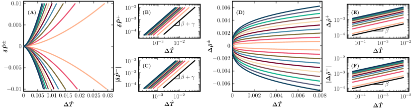
Figure S9: Thermodynamic crossover lines $L^{\pm}$ obtained from the linear scaling theory for asymmetric models ($\varphi=82^{\circ}$). (A) $\delta\hat{P}$ as a function of $\Delta\hat{T}$ along $L^{\pm}$, for $a=0.02,0.04,0.06,0.08,0.1,0.12,0.14,0.16,0.18,0.2$ (from right to left) and $k=a$. The same data are plotted in log-log scales in (B) and (C) for $L^{+}$ and $L^{-}$ respectively, confirming the scaling Eq. (S27). (D) $\Delta\hat{\rho}$ as a function of $\Delta\hat{T}$ along $L^{\pm}$. The same data are plotted in log-log scales in (E) and (F) for $L^{+}$ and $L^{-}$ respectively, confirming the scaling Eq. (S28). The meaning of colors are the same in all panels.

When the slope of the coexistence line is not zero, i.e., $\varphi\neq 0$, it is difficult to obtain an analytical expression of $L^{\pm}$. One has to compute $L^{\pm}$ numerically following the procedure described in Sec. S3. Without loss of generality, we use the following setup: the critical exponents are taken from the 3D Ising model universal class, $\beta\simeq 0.3265$ and $\gamma\simeq 1.237$ [43] (other exponents can be computed using the scaling relations $\alpha+2\beta+\gamma=2$ and $(\delta-1)\beta=\gamma$). The slope of the coexistence line is set to be $\varphi=82^{\circ}$, which is close to that of many real substrates (such as $\mathrm{CO_{2},N_{2}O,CH_{3}F},$ etc.).The parameter $a$ varies from 0.02 to 0.2. To reduce the number of independent parameters, we set $k/a=1$ following previous studies, as suggested by the Monte Carlo simulations of the 3D Ising model with short range interactions [67, 70]. The numerical solution of crossover lines $L^{\pm}$ using the linear scaling theory indeed confirms Eqs. (S27) and (S28), as shown in Fig. S9. We emphasize that these universal scalings are independent of the specific choice of parameters.

Interestingly, the scalings Eqs. (S27) and (S28) remain satisfied if one defines the supercritical crossover lines as the lines of extremums of another response function, such as the isobaric specific heat $C_{P}$ or the isobaric thermal expansion coefficient $\alpha_{P}$. Following a similar procedure as described in Sec. S3, such crossover lines can be also obtained numerically (see Fig. S10). Without loss of generality, we set $\varphi=82^{\circ}$ and $a=k=0.1$. Our results demonstrate that the scalings, Eqs. (S27) and (S28), are independent of which particular response function is used in the definition of $L^{\pm}$. While the scalings are universal, Fig. S11 shows that the supercritical crossover lines defined according to different response functions do not completely coincide, in the regime that is not very close to the critical point.

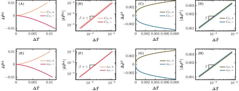
Figure S10: Thermodynamic crossover lines $L^{\pm}$ defined based on other response functions, obtained from the linear scaling theory for an asymmetric model ($\varphi=82^{\circ}$, $a=k=0.1$). (A) $\delta\hat{P}$ as a function of $\Delta\hat{T}$ along $L^{\pm}$ defined according to extreme values of the isobaric specific heat $C_{P}$; (B) same data in log-log scales. (C) $\Delta\hat{\rho}$ as a function of $\Delta\hat{T}$ along $L^{\pm}$ defined according to $C_{P}$; (D) same data in log-log scales. (E-H) Similar to (A-D), but with $L^{\pm}$ defined according to extreme values of the isobaric thermal expansion $\alpha_{P}$. In all case, the scalings Eqs. (S27) and (S28) are satisfied.

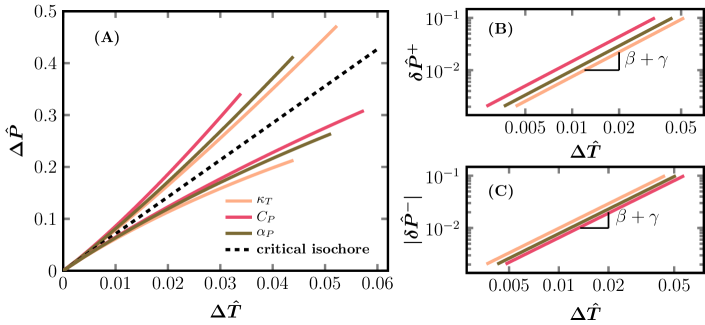
Figure S11: Comparison of $L^{\pm}$ defined according to three different thermodynamic response functions in the linear scaling theory. Results are obtained for $\varphi=82^{\circ}$ and $a=k=0.1$. Same data are plotted in log-log scales in (B) and (C).

S6 Summary of the coefficients $A_{P}^{\pm}$ and $A_{\rho}^{\pm}$ in Fig. 3.

Table S2 summarizes the fitting parameters $A_{P}^{\pm}$ and $A_{\rho}^{\pm}$ for eight different substrates in Fig. 3.

Table S2: Summary of the coefficients $A_{P}^{\pm}$ and $A_{\rho}^{\pm}$ in Fig. 3.

substrates	$\qquad A_{P}^{+}\qquad$	$\qquad A_{P}^{-}\qquad$	$\qquad A_{\rho}^{+}\qquad$	$\qquad A_{\rho}^{-}\qquad$
$\rm{Ar}$	17.31	10.22	0.83	0.97
$\rm{C_{3}H_{8}}$	21.98	15.08	0.85	0.94
$\rm{CO_{2}}$	23.39	13.74	0.88	0.99
$\rm{H_{2}O}$	23.83	15.54	1.06	0.98
$\rm{N}$	18.44	9.97	0.85	0.99
$\rm{N_{2}O}$	22.20	13.50	0.85	0.98
$\rm{Ne}$	16.58	9.99	0.86	0.99
$\rm{O_{2}}$	17.99	10.59	0.83	0.98

S7 Additional data of $L^{\pm}$ lines of argon

S7.1 Examination of different fitting methods

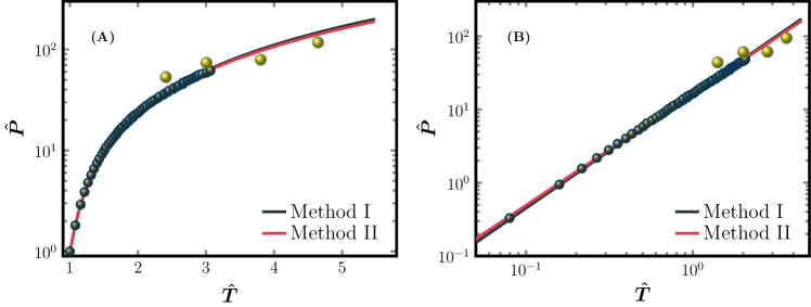
Figure S12: Comparison of the extrapolated $L^{+}$ line of supercritical argon using two different fitting methods. (A) Cycles are obtained by locating maxima of $\kappa_{T}$ using the NIST data. Solid lines with different colors are obtained using two different fitting methods as described in the text. For the first method (I), the resulted fitting parameter is $A_{P}^{+}=16.49$. For the second method (II), the resulted fitting parameters are, $A_{P}^{+}=16.45$ and $\beta+\gamma=1.523$. Same data are plotted in log-log scales in (B). Yellow balls are dynamical crossovers estimated from the sound dispersion data (see Fig. 4).

By definition, $L^{+}$ is determined at the loci of maxima of $\kappa_{T}$ along paths parallel to the isochore. Away from the critical point, the maximum becomes difficult to locate due to the limited range of experimental EOSs. Thus one has to rely on numerical extrapolations to estimate $L^{+}$ at pressures much higher than the critical pressure. Based on the scaling obtained from the above theoretical analysis, we fit the data of $L^{+}$ near the critical point, which are directly determined from the maxima of $\kappa_{T}$ (circles in Fig. 4 and Fig. S12), to,

$$\delta\hat{P}^{+}=A_{P}^{+}\Delta\hat{T}^{\beta+\gamma}.$$ (S33)

Then the fitting curves are extrapolated to the higher pressure regime (lines in Fig. 4 and Fig. S12), in order to have a full comparison with the sound dispersion data. Two fitting methods are considered. In the first method, we set the 3D Ising model universal class critical exponents $\beta+\gamma=0.326+1.237=1.563$, and treat the coefficient $A_{P}^{+}$ as a fitting parameter. In the second method, $\beta+\gamma$ and $A_{P}^{+}$ are treated as two independent fitting parameters. As shown in Fig. S12, the two methods give nearly identical extrapolations in the interested region of the phase diagram.

S7.2 $L^{\pm}$ lines defined by different response functions

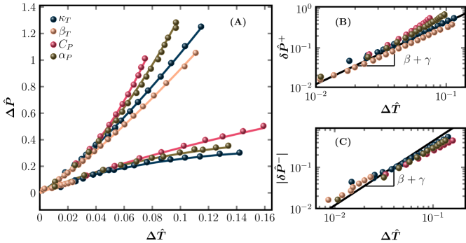
Figure S13: Comparison of the $L^{\pm}$ lines defined according to four different thermodynamic response functions of argon. (A) $L^{\pm}$ lines obtained from the maxima of four different response functions, $\kappa_{T}=\left(\frac{\partial\hat{\rho}}{\partial\hat{P}}\right)_{\hat{T}}$, $\beta_{T}=\frac{1}{\hat{\rho}}\left(\frac{\partial\hat{\rho}}{\partial\hat{P}}\right)_{\hat{T}}$, $C_{P}=\hat{T}\left(\frac{\partial\hat{S}}{\partial\hat{T}}\right)_{\hat{P}}$, and $\alpha_{P}=-\frac{1}{\hat{\rho}}\left(\frac{\partial\hat{\rho}}{\partial\hat{T}}\right)_{\hat{P}}$. (B) and (C) are the same data in log-log scales for $L^{+}$ and $L^{-}$ respectively. Solid lines represent the scaling $\delta\hat{P}^{\pm}\sim\Delta\hat{T}^{\beta+\gamma}$ with $\beta+\gamma=1.563$.

Here we check that if $L^{\pm}$ lines can be defined using other response functions (see Fig. S13). As shown in Fig. S13A, even though these lines do not completely coincide, the discrepancies reduce approaching the critical point. Further more, they follow the same scaling (Fig. S13B and C), consistent with the theoretical results calculated using the linear scaling theory (see Fig. S11). Unlike phase transition lines where all response functions are singular, the thermodynamical crossover lines $L^{\pm}$ defined by different response functions are not unique, except for the universal scalings. When the crossover line is compared to experimental data, one should choose a proper response function suitable for the given experiment. For example, in the inelastic X-ray scattering experiment, the measured data of sound speed and dispersion are essentially related to density fluctuations [2, 1]; thus is is reasonable to choose $\kappa_{T}$ to define $L^{\pm}$ in order to compare with the data (see Fig. 4 and Sec. S8).

S8 Reestimation of dynamical crossovers in supercritical argon from sound dispersion data

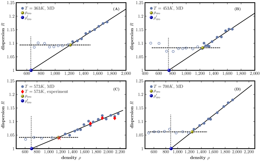
Figure S14: Re-estimation of dynamical crossovers in supercritical argon, based on the sound dispersion data collected from [2, 1]. Sound dispersion $R$ as a function of density $\rho$ at four different temperatures. Open and filled circles are data points obtained from molecular dynamics (MD) simulations in  [2, 1]. Open circles are fitted to a constant (horizontal dashed line); filled circles are fitted to a linear function (solid line). The intersection of dashed and solid lines defines the crossover density $\rho_{\rm cro}$. The intersection between the solid line and the $R=1$ axis defines $\rho^{\prime}_{\rm cro}$, according to Ref. [2]. Red diamonds in (C) represent experimental data and the red star represents the crossover estimated in  [1].

We collect experimental and simulation sound dispersion data of supercritical argon from the literature [2, 1], and re-analyze them to obtain supercritical crossovers. The data are reported at four temperatures, 363 K ($2.4T_{\rm c}$), 453 K ($3T_{\rm c}$), 573 K ($3.8T_{\rm c}$) and 700 K ($4.6T_{\rm c}$). Several data points at $T=573K$ are obtained from inelastic X-ray scattering experiments in [1] (see Fig. S14); other data points are obtained from molecular dynamics (MD) simulations in [2, 1]. In Fig. S14, we plot the positive dispersion ratio $R=c_{\rm L}^{\rm max}/c_{\rm s}$ as a function of density $\rho$, where $c_{\rm L}^{\rm max}$ is the maximum of $c_{\rm L}(Q)$, $c_{\rm s}=c_{\rm L}(Q\to 0)$ is the adiabatic sound velocity, and $c_{\rm L}(Q)$ is the longitudinal sound velocity as a function of the wave number $Q$. A zero value of $R$ means the absence of dispersion.

In Ref. [1], a supercritical dynamical crossover is defined as the separation between a gas-like regime, where $R\approx 1.04$ is a small constant, and a liquid-like regime, where $R$ increases with the pressure $P$, under a fixed temperature $T=573$ K. We follow this definition to evaluate the crossover points at other temperatures. Specifically, we fit $R(\rho)$ to a linear function at large $\rho$, and a constant at small $\rho$. The intersection of the two lines determines the crossover density $\rho_{\rm cro}$. Such a method is in fact commonly used in the evaluation of other dynamical crossovers, e.g., the evaluation of liquid-glass transition temperature $T_{\rm g}$ from heat capacity data. Once $\rho_{\rm cro}(T)$ is available, $P_{\rm cro}(T)$ can be computed according to the EOSs provided by the NIST database. Note that our estimated crossover at $T=573$ K is fully consistent with the value reported in  [1].

In Ref. [2], the authors use another definition to evaluate the supercritical crossovers. The linear fitting of $R(\rho)$ at large $\rho$ is extended to lower $\rho$; the intersection between this linear extrapolation and the horizontal line $R=1$ defines $\rho_{\rm cro}^{\prime}$. As can be seen in Fig. S14, $\rho_{\rm cro}^{\prime}$ obtained in this way is already in the constant $R(\rho)$ regime, and therefore might underestimate the crossover density. Note that the criterion $R=1$ (i.e., the complete absence of dispersion) is assumed for the gas or gas-like regime in Ref. [2]. However, according to our phase diagram (Fig. 4), the constant $R(\rho)$ data are in the liquid-gas indistinguishable regime, rather than in the gas-like regime. There is no particular reason to assume that the dispersion is completely absent in the indistinguishable regime: the differences on the acoustic properties of the indistinguishable and gas-like regimes remain to be explored in future studies.

Based on above discussions, we find that $\rho_{\rm cro}$ is a more reliable and accurate estimation of the supercritical crossover density than $\rho_{\rm cro}^{\prime}$. Thus the former is adopted in this study.

S9 Comparison of different supercritical crossover lines of argon in the vicinity of the critical point

In Fig. S15, we compare $L^{\pm}$ lines with other crossover lines of supercritical argon near the critical point. This is an enlarged view of Fig. 4(A) in the vicinity of the critical point, presented in linear scales.

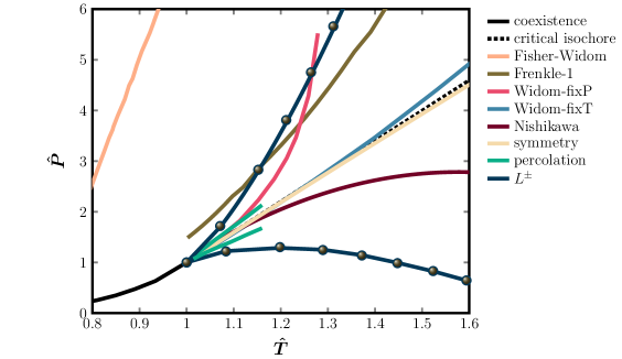
Figure S15: Different supercritical crossover lines of argon in the vicinity of the critical point. This is an enlarged view of Fig. 4(A), and all symbols and colors represent the same meanings as in Fig. 4(A).

S10 Nishikawa line of argon

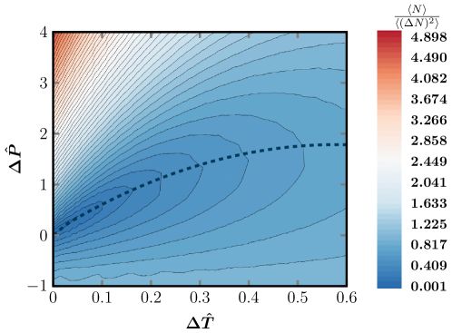
Figure S16: Colormap of the density fluctuation $\frac{\langle(\Delta N)^{2}\rangle}{\langle N\rangle}$ in the $P$-$T$ phase diagram. Thin solid lines are constant density fluctuation lines. The dashed black line is the ridge that defines the Nishikawa line.

Because the Nishikawa line of argon is not available in the literature, here we estimate it according to its definition. The Nishikawa line is determined by the “ridge” of density fluctuations $\frac{\langle(\Delta N)^{2}\rangle}{\langle N\rangle}$ on the $P-T$ phase diagram. The density fluctuation can be computed from EOSs using the following formula [38]:

$$\frac{\langle(\Delta N)^{2}\rangle}{\langle N\rangle}=RT\rho\beta_{T},$$ (S34)

where $R$ is universal gas constant. The data of argon isotherms are collected from the NIST database. Figure S16 shows the colormap and contour lines of density fluctuations on $P-T$ phase diagram, where the Nishikawa line is determined as the ridge of contour lines. The Nishikawa line plotted in Fig. 4(A) is obtained in this way.

S11 Validation of $L^{-}$ line by the equation of states for the compressibility factor

We show that the $L^{-}$ line can be validated by the behavior of EOS that relates compressibility factor $Z=PV/nRT$ to $\hat{\rho}$ and $\hat{T}$, where $n$ is the number of moles. Specifically, the supercritical gas-like states at different $\hat{T}$ obey a single EOS,

$$Z_{\rm gas}(\hat{\rho},\hat{T})-1=\mathcal{F}\left[\hat{\rho}/\rho^{*}(\hat{T})\right],$$ (S35)

and that the $L^{-}$ line coincides with the points where the actual EOS starts to deviate from this gas form. We first derive Eq. (S35) from the van der Waals equation Eq. (S11), which can be rewritten as,

$$Z_{\rm vdW}(\hat{\rho},\hat{T})=\frac{1}{1-\frac{1}{3}\hat{\rho}}-\frac{9\hat{\rho}}{8\hat{T}}.$$ (S36)

In the dilute gas limit $\rho\to 0$, it can be expanded as,

$$Z_{\rm vdW}(\hat{\rho},\hat{T})\approx 1+\frac{\hat{\rho}}{3}-\frac{9\hat{\rho}}{8\hat{T}}.$$ (S37)

Equation (S37) satisfies the form of Eq. (S35), with $\rho^{*}(\hat{T})=24\hat{T}/(27-8\hat{T})$ and $\mathcal{F}(x)\approx-x$. For larger $\hat{\rho}$, Eq. (S35) is still obeyed, with a modified $\mathcal{F}(x)\approx-x+0.24x^{2}$ that can be obtained from fitting (see Fig. S17A). The modification to the dilute-gas EOS with $\mathcal{F}(x)\approx-x$ implies corrections required for high-density gas-like states. At even larger $\hat{\rho}$, Eq. (S35) can no longer be satisfied by modifying $\mathcal{F}(x)$. For a given $\hat{T}$, the point where the original van der Waals EOS Eq. (S36) deviates from the gas form Eq. (S35) coincides with the $L^{-}$ line, as shown in Fig. S17(A). This result is consistent with our definition of $L^{-}$ line: below the line the system is in the gas-like state that can be described by a uniform EOS Eq. (S35); above the line the system enters into the liquid-gas indistinguishable state and thus the gas-like EOS Eq. (S35) does not hold anymore.

We find that the NIST data of argon also follow Eq. (S35) with $\rho^{*}(\hat{T})=1/(-0.57+1.51/\hat{T})$ and $\mathcal{F}(x)\approx-x+0.28x^{2}$ in the gas-like regime, as shown in Fig. S17(B). For each $\hat{T}$, the gas-like regime begins from the ideal gas limit ($\rho\to 0$) and terminates at a point where the EOS deviates from Eq. (S35). The deviation points can be considered as an independent determination of the $L^{-}$ line, coinciding with those defined in Fig. 2.

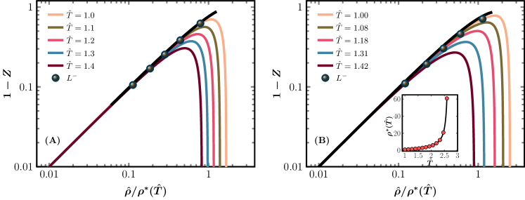
Figure S17: Validations of the $L^{-}$ line by the equation of states for the compressibility factor. (A) Van der Waals EOS. Colored lines are isotherms and the black line is Eq. (S35) with $\rho^{*}(\hat{T})=24\hat{T}/(27-8\hat{T})$ and $\mathcal{F}(x)=-x+0.24x^{2}$. (B) NIST data of argon. Colored lines are isotherms and the black line is the fitted gas-like EOS Eq. (S35) with $\mathcal{F}(x)=-x+0.28x^{2}$. The points of $L^{-}$ line are determined independently in Fig. 2, which coincide with the deviation points as shown in the plot. The inset shows $\rho^{*}(\hat{T})$ as a function of $\hat{T}$, where the solid line represents $\rho^{*}(\hat{T})=1/(-0.57+1.51/\hat{T})$ obtained from fitting.