HyperINR: A Fast and Predictive Hypernetwork for Implicit Neural Representations via Knowledge Distillation

Abstract

Implicit Neural Representations (INRs) have recently exhibited immense potential in the field of scientific visualization for both data generation and visualization tasks. However, these representations often consist of large multi-layer perceptrons (MLPs), necessitating millions of operations for a single forward pass, consequently hindering interactive visual exploration. While reducing the size of the MLPs and employing efficient parametric encoding schemes can alleviate this issue, it compromises generalizability for unseen parameters, rendering it unsuitable for tasks such as temporal super-resolution. In this paper, we introduce HyperINR, a novel hypernetwork architecture capable of directly predicting the weights for a compact INR. By harnessing an ensemble of multiresolution hash encoding units in unison, the resulting INR attains state-of-the-art inference performance (up to $100\times$ higher inference bandwidth) and supports interactive photo-realistic volume visualization. Additionally, by incorporating knowledge distillation, exceptional data and visualization generation quality is achieved, making our method valuable for real-time parameter exploration. We validate the effectiveness of our HyperINR architecture through a comprehensive ablation study. We showcase the versatility of HyperINR across three distinct visualization tasks: novel view synthesis, temporal super-resolution of volume data, and volume rendering with dynamic global shadows. By simultaneously achieving efficiency and generalizability, HyperINR paves the way for applying INR in a wider array of scientific visualization applications.

Comparisons between HyperINR and data interpolation for the temporal super-resolution task using the vortices dataset. Listed timesteps are midpoints of different interpolation intervals. HyperINR can directly predict the weights of a regular implicit neural representation (INR) for unseen parameters. The predicted INR is in general more accurate than data interpolation results and can support interactive volumetric path tracing.

Introduction

In the field of scientific visualization, continuous fields are often represented using discrete data structures such as grids, unstructured meshes, or point clouds. These structures are limited by resolution and can be cumbersome to handle due to their complexity. To address this, Lu et al. [23] introduced an alternative approach, employing a continuous function modeled using a fully connected multi-layer perceptron (MLP) to implicitly represent data fields. Such an implicit neural representation (INR) offers several key advantages, including substantial data size reductions while preserving high-frequency details, and direct access to spatial locations at arbitrary resolutions without decompression or interpolation. A recent advancement in INR is CoordNet, introduced by Han et al. [14], which generalizes INR to incorporate simulation parameters ($\theta_{sim}$) and visualization parameters ($\theta_{vis}$) for predictive tasks such as temporal super-resolution or visualization synthesis. With a well-designed fully connected INR and a suitable activation function, CoordNet generates more meaningful results than direct data interpolation for previously unseen parameters. However, a single pass through such a large fully connected INR may require millions of operations, making it slow for neural network inference and thus unsuitable for interactive visualizations.

Wu et al. [48] and Weiss et al. [47] addressed the challenge of long inference times of large fully connected INRs by reducing the neural network size to approximately 200 neurons and incorporating additional trainable parameters through auxiliary data structures to compensate for the reduction in network capacity. Such auxiliary data structures are typically constructed in the form of hash tables [28] or octrees [40], and are responsible for transforming input coordinates into high-dimensional vectors, a process known as parametric positional encoding. Compared with parameters stored in the neural network, querying, interpolating, and optimizing encoding parameters based on input coordinates can be performed more rapidly. Consequently, interactive visualization of INR models can be achieved. However, the majority of data features are strongly embedded into the trainable encoding parameters rather than being generalized by the MLP. In turn, the generalizability of INR in regards to unseen data is significantly reduced. Therefore, a method that can offer strong generalizability while still maintaining exceptional inference performance for enabling interactive visualization and real-time parameter exploration is highly desirable.

In this paper, we present HyperINR, a hypernetwork designed to conditionally predict the weights of an Implicit Neural Representation (INR) using multiple compact multiresolution hash encoders [28] and incorporating a deeply embedded weight interpolation operation. These hash encoders correspond to points in the parameter space and are organized within a spatial data structure. Given an input, the data structure is traversed to gather a set of nearest hash encoders, whose weights are subsequently interpolated based on the input and combined with the weights of a shared MLP common to all encoders. This combined weight is then suitable for use as an INR, enabling interactive volumetric path tracing through the state-of-the-art INR rendering algorithm proposed by Wu et al. [48], with the INR generation process taking less than 1ms to complete (up to $100\times$ faster than CoordNet). Furthermore, we optimize HyperINR using knowledge distillation, leveraging CoordNet [14] as the teacher model, to achieve state-of-the-art generalizability for unseen parameters, rendering HyperINR suitable for real-time parameter exploration. We conduct a comprehensive evaluation of HyperINR’s architecture through an extensive ablation study and assess its performance in three distinct scientific visualization tasks: Novel View Synthesis (NVS), Temporal Super-Resolution of Volume Data (TSR), and Volume Rendering with Dynamic Global Shadows (DGS). Our contributions can be summarized as follows.

• We design HyperINR: A hypernetwork that efficiently generates the weights of a regular INR for given parameters, achieving state-of-the-art inference performance and enabling high-quality interactive volumetric path tracing.

• We introduce a framework for optimizing HyperINR through knowledge distillation, attaining state-of-the-art data generalization quality for unseen parameters and supporting real-time parameter exploration.

• We demonstrate HyperINR’s exceptional inference performance and its ability to generate meaningful data and visualizations across a diverse range of scientific visualization tasks.

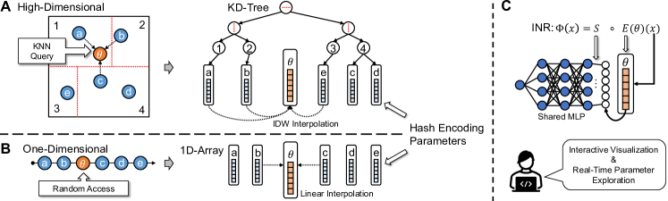
Figure 1: The architecture of HyperINR. HyperINR is composed of a shared MLP denoted as $S$ and a collection of multiresolution hash encoding parameters $E$, with each parameter associated with a set of values $\{a,b,c,...\}$. A) In high dimensions, a KD-tree is utilized, B) while in 1D, the encoding parameters are arranged in a linear array. C) The input parameter $\theta$ is utilized to query the data structure, and the queried encoding parameters are interpolated and combined with the shared MLP to construct an INR. The resulting INR enables interactive visualization and real-time parameter exploration.

1 Related Work

In this related work section, we delve into the relevant research areas related to our presented work. We begin by providing an overview of recent advancements in generation models for scientific visualization, followed by a review of implicit neural representation. Because our technique involves hypernetwork and knowledge distillation, we also review the latest advancements in these areas.

1.1 Generation Models for Scientific Visualization

Using neural networks to generate new data or visualization that are similar to the training data has been studied by many in recent years. We overview related in this area, and we refer to Wang et al. [45] for a more comprehensive survey of this topic.

For visualization generation, Berger et al. [3] developed a generative adversarial network (GAN) for synthesizing volume rendering images with different transfer functions and view parameters. GAN was also used by He et al. [17] to create a simulation and visualization surrogate model called InSituNet for exploring ensemble simulation parameters. Engel and Ropinski [7] built a 3D U-Net that can predict local ambient occlusion data for given transfer functions. Weiss et al. [46] proposed a convolutional neural network (CNN) network to coherently upscale isosurface images by training the network using depth and normal information. Han and Wang [15] developed a GAN-based volume completion network for visualizing data with missing subregions. Bauer et al. [2] introduced a CNN-based screen space method that enables faster volume rendering through sparse sampling and neural reconstruction.

For data generation, Zhou et al. [51] and Guo [9] designed CNNs for upscaling scalar and vector field volume data respectively. Han and Wang employed GANs for generating time-varying volume data at higher temporal [12] or spatial et al. [13] resolutions. Han et al. [16] later also presented an end-to-end solution for achieving both goals at the same time. Shi et al. [36] improved InSituNet through view-dependent latent-space generative models, and their method can directly predict simulation data rather than being bound to the visualization strategy used for generating the training data. Data generation models are also applicable to volume compression. Jain et al. [19] presented an encoder-decoder network to compress a high-resolution volume. Wurster et al. [49] developed a hierarchical GAN for the same task.

Very recently, Han et al. [14] explored the use of implicit neural representation and proposed CoordNet for both data and visualization generation tasks. In our work, we use CoordNet as the teacher model for knowledge distillation.

1.2 Implicit Neural Representation (INR)

In the field of scientific visualization, Lu et al. [23] first explored the use of INR for volume compression. Their network utilizes multiple ResNet blocks and the sine activation function to achieve high reconstruction qualities. Previously mentioned CoordNet by Han et al. [14] for time-varying data is also worth mentioning here. CoordNet can be considered as a conditional-INR. However, their method requires a time-consuming training process for every volume data, and more crucially, the network is slow for inference. Wu et al. [48] and Weiss et al. [47] addressed these issues using parametric positional encoding [40, 28] and GPU-accelerated inference routines. Wu et al.also proposed an auxiliary data structure to enable interactive volume rendering and an optimized algorithm for computing global illuminations. In this work, we adopt the INR architecture proposed by Wu et al.as the base. We develop our interactive volume visualization algorithms based on their proposals. INR can also be used in hybrid with other hierarchical data structures. Doyub et al. [20] recently demonstrated this for handling high-resolution sparse volumes.

Positional encoding converts an input coordinate to a higher-dimension vector before being passed to subsequent layers. It allows the network to capture high-frequency local details better. Positional encoding was proven to be helpful in the attention components of recurrent networks [8] and transformers [43], and later adopted by NeRF [26] and many INR-based works [41, 1, 29] in computer graphics. To further optimize training time and improve accuracy, parametric positional encoding was introduced. It introduces an auxiliary data structures such as dense grids [24], sparse grids [11], octrees [40], or multiresolution hash tables [28] to store training parameters. Thus, the neural network size can be reduced. Therefore neural networks with such encoding methods can typically converge much faster. In this work, we adopt the multiresolution hash grid method proposed by Müller et al. [28] due to its excellent performance.

1.3 Hypernetwork for INR

Hypernetworks or meta-models are networks that generate weights for other neural networks [10]. They have a wide range of applications, including few-shot learning [4], continual learning [44], architecture search [50], and generative modeling [33, 31, 32], among others. Hypernetworks can also be combined with implicit neural representations (INRs). For instance, Klocek et al. [21] developed an INR-based hypernetwork for image super-resolution. DeepMeta [22] builds a hypernet that takes a single-view image and outputs an INR. Skorokhodov et al. [39] developed a GAN-based hypernet for continuous image generation. Sitzmann et al. [38] proposed an MLP-based hypernetwork to parameterize INRs for 3D scenes consisting of only opaque surfaces. In this work, we utilize hypernetworks to build a large neural network that has the potential to learn an ensemble of data while maintaining the capability of interactive volume visualization.

2 Formulation for HyperINR

INRs can be regarded as functions mapping 2D or 3D coordinates $\vec{x}$ to their corresponding field values $\vec{v}$:

$$\Phi:\vec{x}\mapsto\Phi(\vec{x})=\vec{v},\leavevmode\nobreak\ \vec{x}\in\mathbb{R}^{2}\leavevmode\nobreak\ \text{or}\leavevmode\nobreak\ \mathbb{R}^{3}.$$ (1)

We employ $\Phi$ for approximating image or volume data $V$ that are intrinsically parameterized by a scene parameter (e.g., timestep, lighting direction) from a high-dimensional parameter space $\Theta$. Our objective is to construct a neural network capable of continuously generating such an INR based on parameters in $\Theta$, using a sparsely sampled training set $\mathcal{C}=\{V(\theta_{i}),\leavevmode\nobreak\ \theta_{i}\}$. The resulting INR is expected to be suitable for interactive visualization and real-time parameter exploration. Formally, such a neural network can be defined as a higher-order function, $S$, which accepts scene parameters $\theta$ as inputs, and yields $\Phi$ conditioned on these parameters:

$$H(\theta)(\vec{x})=\Phi(\vec{x}\leavevmode\nobreak\ |\leavevmode\nobreak\ \theta)\in V(\theta),\leavevmode\nobreak\ \text{for}\leavevmode\nobreak\ \theta\in\Theta,\leavevmode\nobreak\ \forall\leavevmode\nobreak\ \vec{x}\in\mathbb{R}^{2}\leavevmode\nobreak\ \text{or}\leavevmode\nobreak\ \mathbb{R}^{3}.$$ (2)

To incorporate the state-of-the-art rendering algorithm by Wu et al. [48] for interactive 3D visualization of INRs, we further decompose $\Phi$ into two distinct functions: an encoding function $E$, mapping input coordinates to high-dimensional vectors via a multiresolution hash encoder; and a synthesis function $S$, converting the high-dimensional vectors into data values parameterized by an MLP:

$$\Phi(\vec{x}\leavevmode\nobreak\ |\leavevmode\nobreak\ \theta)=S\circ E(\theta)(\vec{x}).$$ (3)

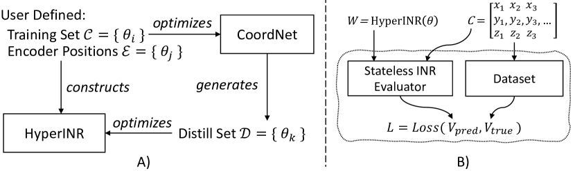
Figure 2: A) Visualization of the knowledge distillation process, wherein a user provides a training set $\mathcal{C}$ and a set of encoder positions $\mathcal{E}$. We utilize $\mathcal{C}$ to pretrain CoordNet and construct HyperINR using $\mathcal{E}$. Following pretraining, we create a distillation set $\mathcal{D}$ and optimize HyperINR using it. B) We introduce a stateless INR evaluator for end-to-end training of the hypernetwork, leading to improved training quality.

In our work, we utilize a shared synthesis function $S$ for all scene parameters, intentionally designed to significantly enhance training robustness, as demonstrated through our experimental results in Section 5.2. Thus, the primary objective of HyperINR becomes predicting the encoding function $E$ for a given set of parameters $\theta$. As illustrated in Figure 1, we first sample $N$ scene parameters $\mathcal{E}=\{\theta_{j}\leavevmode\nobreak\ |\leavevmode\nobreak\ j=a,b,c,...\}$ and construct a multiresolution hash encoder $E_{j}=E(\theta_{j})$ for each $\theta_{j}$. We refer to $\mathcal{E}$ as encoder positions and organize them using a KD-tree based on these positions. Given a set of parameters $\theta$, we traverse the KD-tree to gather the $K$ nearest encoders around $\theta$ and interpolate their weights using inverse distance weighting (IDW), also known as Shepard’s algorithm [35]:

$$E(\theta)=\begin{cases}\sum_{j=1}^{N}\frac{w_{j}E_{j}}{\sum_{i=j}^{N}\leavevmode\nobreak\ w_{j}}&\text{if }d(\theta,\theta_{i})\neq 0,\leavevmode\nobreak\ \forall\leavevmode\nobreak\ j\\ E_{j}&\text{if }d(\theta,\theta_{j})=0,\end{cases}$$ (4)

where $w_{j}=d(\theta,\theta_{j})^{-p}$ with $p=1$. If the scene parameter space $\Theta$ is one-dimensional, a fast-path is provided by replacing the KD-tree with a linear array and performing linear interpolation instead of IDW.

Importantly, encoder positions $\mathcal{E}$ can be distinct from the training set $\mathcal{C}$. We combine Bridson’s fast Poisson Disk sampling algorithm [5] and Gaussian kernel sampling to generate $\mathcal{E}$. Poisson Disk Sampling ensures even distribution of encoders in the parameter space, maintaining a minimum distance between encoders while preventing regular grid-like patterns. Gaussian kernel sampling enables integration of application-specific knowledge into the network. In Section 5.4, we perform an ablation study to analyze the impact of $\mathcal{E}$ on the network’s generalization capabilities.

2.1 Organize Weight Space via Knowledge Distillation

Knowledge distillation is a powerful method for knowledge transfer between models, with early demonstrations by Buciluă et al. [6] and subsequent formalizations by Hinton et al. [18]. In this study, we leverage knowledge distillation to enhance the performance of HyperINR by employing a fully-connected conditional INR with strong generalizability as the teacher model. The process begins with training the teacher model, denoted as $\Omega$, on the training set. Then, a distillation set $\mathcal{D}$ is created by strategically sampling a set of scene parameters $\{\theta_{k}\}$, and computing the corresponding data $\{\Omega(\theta_{k})\}$ using the trained teacher model. Finally, the HyperINR is optimized using $\mathcal{D}$. A visual illustration of this process can be found in Figure 2.

The distillation set $\mathcal{D}$ can be pre-computed or generated on-demand. Pre-computing $\mathcal{D}$ avoids the training process being bottlenecked by the inference bandwidth of the teacher model, while generating $\mathcal{D}$ on-demand can greatly reduce memory usage. In this work, we pre-compute $\mathcal{D}$. Furthermore, the selection of a high-quality teacher model and the construction of the distillation set $\mathcal{D}$ can be critical for producing a good HyperINR. In our work, we choose CoordNet as the teacher model due to its remarkable data generation capability.

2.2 Multiresolution Hash Encoding

Table 1: Datasets Used in All Tasks

Data	Count	Dimensions	Input/Output	Task
Vortices	100	$128,128,128$	$(t,x,y,z)\mapsto v$	TSR
Pressure	105	$128,128,128$	$(t,x,y,z)\mapsto v$	TSR
Temp	100	$864,240,640$	$(t,x,y,z)\mapsto v$	TSR
MPAS	200	$256,256$	$(\theta,\phi,x,y)\mapsto(r,g,b)$	NVS
MechHand	150	$256,256,256$	$(\theta,\phi,x,y,z)\mapsto v$	DGS

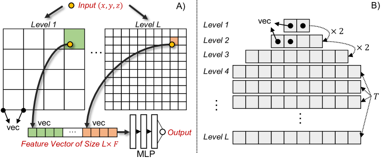
Figure 3: Multiresolution Hash Encoding: A) The encoding process and the virtual grids represented by the hash encoding. B) The actual data arrangement within the hash encoding.

Multiresolution hash encoding [28] is a key technique that enables interactive visualization for our approach. This method models the encoding function $E$ using $L$ levels of independent hash tables with each containing up to $T$ feature vectors of length $F$. Each level conceptually corresponds to a virtual grid with feature vectors stored at its vertices. Figure 3A illustrates the steps performed in the encoding process.

The grid resolution $R_{l}$ starts at a base value $R_{1}$ and increases progressively ($\times 2$ in this paper) as the level $l$ increases. Input coordinates are expected to be normalized to $[0,1]^{d}$, and then scaled to the grid’s resolution: $\vec{x_{l}}=\vec{x}\cdot R_{l}+0.5$. The offset of 0.5 causes different scales to be staggered with respect to each other, thus preventing spurious alignment of fractional coordinates upon integer scales. The output encoding at this level is calculated by interpolating grid vertices based on $x_{l}$. In this paper, we use linear interpolation.

Figure 3B highlights how trainable parameters are stored in the data structure. The grid resolution $R_{l}$ starts from a relatively small base value, and the number of vertices at this level might be smaller than $T$. In this case, encoding parameters are directly organized as a linear. When the number of vertices becomes greater than $T$, a spatial hash function is used to condense encoding parameters. The hash function used is given by:

$$\text{hash}(\vec{x})=\left(\oplus_{i=1}^{d}x_{i}\pi_{i}\right),$$ (5)

where $\oplus$ is a bitwise XOR operation and $\pi_{i}$ are unique, large prime numbers. Based on Müller et al. [28]’s recommendation, we use $\pi_{1}=1$, $\pi_{2}=2\leavevmode\nobreak\ 654\leavevmode\nobreak\ 435\leavevmode\nobreak\ 761$, and $\pi_{3}=805\leavevmode\nobreak\ 459\leavevmode\nobreak\ 861$. Since multiresolution hash encoding is designed to encode spatial coordinates, only 3 prime numbers are used.

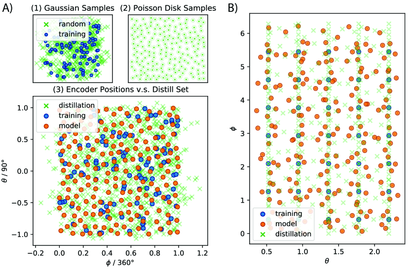
Figure 4: A) The visualization of encoder positions $\mathcal{E}$ and the distillation set $\mathcal{D}$ for the novel view synthesis task. We generated encoder positions using Poisson disk sampling (2). We generated distillation set also using Poisson disk sampling, but combined with Gaussian kernel sampling (1). We centered Gaussian kernels on training set. B) The same visualization for the dynamic global shadow task. In this task, we also included some distillation parameters sampled uniformly in the parameter space.

3 Applications

In this paper, we apply HyperINR to three common generative tasks in scientific visualization, namely novel view synthesis (NVS), temporal super resolution (TSR), and dynamic global shadows for volume rendering (DGS). Detailed descriptions of setups and datasets used for each task are provided below. In addition, the usages of the datasets are summarized in Table 1.

Novel View Synthesis

The objective of NVS is to generate meaningful and visually coherent images of a scene from previously unobserved viewpoints or perspectives, utilizing a collection of pre-existing images. NVS holds significant potential in the realm of scientific visualization, enabling the creation of explorable images [42]. To perform this task, an INR should accept two spatial inputs $(x,y)$ and a viewing direction, subsequently producing an RGB color $(r,g,b)$. In this study, we parameterize the viewing direction using a spherical coordinate system, characterized by a polar angle $\theta$ and an azimuthal angle $\phi$. Our experiment employs a dataset of 200 isosurface visualizations, generated by He et al. [17] utilizing the MPAS-Ocean simulation from the Los Alamos National Laboratory, referred to as the MPAS dataset. 100 of the visualizations were allocated for training, and the remaining were for testing purposes. Furthermore, the quality of the synthesized images was assessed through the Peak Signal-to-Noise Ratio (PSNR) metric. The model’s inference performance was evaluated in terms of the data bandwidth.

Temporal Super Resolution

The goal of TSR is to train a neural network on a sequence of sparsely sampled time-varying volume data and enable the generation of the same sequence at a higher temporal resolution. A more complete review of related TSR techniques can be found in Section 1.1. We focus on scalar field volume data, where an INR receives a 4D input $(x,y,z,t)$ and outputs a scalar value $v$. Although all of our experiments assumes $v$ to be a scalar value, our method can be extended to multivariate volume data without any alterations to the design. We assess our approach using three datasets: 1) a time-varying simulation of vortices provided by Deborah Silver at Rutgers University, consisting of 100 timesteps with 20 equally spaced steps used for training; 2) the pressure field of a Taylor-Green Vortex simulation generated by the NekRS framework, containing 105 timesteps with 21 selected for training; and 3) the temperature field from a 1atm flame simulation produced by S3D [34], which includes 90 timesteps with 10 employed for training. To evaluate the quality of the generated data, we employ metrics such as PSNR and the Structural Similarity Index Measure (SSIM). For assessing the inference performance, we measure the average inference bandwidth as well as the interactive volume visualization framerates.

Dynamic Global Shadows

Direct volume rendering with global shadows is a non-physically based shading technique widely employed in scientific volume rendering. It enhances realism and helps distinguish features in the data. However, the technique also imposes a significant runtime cost over simple ray casting, as it generates at least one secondary ray towards the light source at each sample point to estimate shadow coefficients. This results in an $O(n^{2})$ computation for each primary ray. An alternative approach involves precomputing all secondary rays at voxel centers, generating a volume data containing shadow coefficients. This “shadow volume” is subsequently utilized to estimate shadow coefficients at sample positions. Although this method reduces the computational complexity to $O(n)$ per ray, it substantially increases the memory footprint for rendering. Furthermore, the shadow volume must be regenerated whenever the transfer function or the light changes, presenting challenges for interactive exploration.

In this work, as a preliminary study, we examine the potential of achieving dynamic global shadows using HyperINR. Specifically, we propose substituting shadow volumes with regular INRs and estimating shadow coefficients through network inferences. We term these INRs as shadow INRs. This optimization significantly reduces memory footprints. Then, we optimize a HyperINR to generate such INRs. The resulting HyperINR can achieve dynamism for global shadows as the generation process can be done in real-time. We validate this method by generating a set of 150 shadow volumes sampled with varying light positions. For this preliminary study, we fix the transfer function and incorporate only one light source. Then, we utilize 35 evenly distributed shadow volumes to optimize our network. To assess the shadow generation quality, we computed the PSNR and SSIM against the ground truth data. To evaluate the inference performance, we measured the rendering framerate and INR generation latency.

4 Implementation

Our network is implemented in PyTorch, with GPU-accelerated training using the Tiny-CUDA-NN machine learning framework [27]. We leverage multiresolution hash encoding for training the INR.

Architecture

HyperINR’s base hash encoder consists of $L=8$ encoding levels, with each level containing up to $T=2^{15}$ feature vectors of size $F=4$. We selected these hyperparameters based on the results presented in Section 5.4. The base grid resolution is set to $R_{1}=8$ for the NVS task and $R_{1}=4$ for TSR and DGS tasks. The MLP unit adopts the configuration proposed by Wu et al. [48], which uses four hidden layers and a width of 64 neurons. This configuration is suitable for the volume rendering algorithm.

As for encoder positions $\mathcal{E}$, 177 encoder positions were randomly generated using Poisson disk sampling within a $[0,1]^{2}$ space for the NVS task, 24 encoding units were evenly distributed across the temporal domain for the TSR task, and 206 encoder positions were created using both Poisson disk sampling and Gaussian distribution sampling for the DGS task. The impact of these hyperparameters is further explored in Section 5.4.

Distillation

We select CoordNet as the teacher model for knowledge distillation. However, since a reference implementation of CoordNet is not publicly available, we implement it based on SIREN [37] and NeurComp [23]. Our implementation closely matches the architecture described in the CoordNet paper [14]: we use 3 resblocks as the encoder to process inputs, 10 hidden resblocks of size 256, and 1 resblock as the decoder to produce final outputs. It is worth noting that CoordNet expects input and output values to be within the range of $[-1,1]$, whereas hash-encoding-based INRs use a range of $[0,1]$. Therefore, in our implementation, we use $[0,1]$ as the value range and only convert it to the $[-1,1]$ range when interacting with CoordNet.

Training

We develop an end-to-end training framework to optimize our hypernetwork instead of relying on pre-trained network weights. To achieve this, we implement a stateless INR evaluator (as shown in Figure 2) that takes a coordinate matrix $C$ and a network weight matrix $W$ predicted by the hypernetwork as inputs, and generates output data $V_{\text{pred}}$. A loss is thus calculated with respect to the ground truth $V_{\text{true}}$. Then the evaluator can compute gradients with respect to $W$ and backpropagate them to the hypernetwork. For NVS, we use the $\mathcal{L}^{2}$ loss between pixel colors. For TSR and DGS, we use the $\mathcal{L}^{1}$ loss following the recommendations of Han et al. [14].

To optimize HyperINR, we use the Adam optimizer with $\beta_{1}=0.9$, $\beta_{2}=0.999$, and $\epsilon=10^{-10}$. A good convergence speed was observed with a learning rate of $10^{-3}$. The teacher model, CoordNet, was also trained using the Adam optimizer with $\beta_{1}=0.9$, $\beta_{2}=0.999$, $\epsilon=10^{-8}$, and a weight decay of $10^{-6}$. We find that CoordNet can be sensitive to the learning rate and a learning rate of $10^{-5}$ enables stable convergence. For NVS, we optimize CoordNet for 300 epochs and then create a distillation set $\mathcal{D}$ using a combination of Poisson disk sampling and Gaussian kernel sampling, similar to the generation of encoder positions. The $\mathcal{D}$ is visualized in Figure 4A. For TSR tasks, we train CoordNet for 30k epochs to ensure good performance for the teacher model. Then, we create distillation sets by uniformly sampling the time axis. For the DGS task, we also train CoordNet for 30k epochs but generate a $\mathcal{D}$ containing 400 samples, which is visualized in Figure 4B. Table 2 contains the summary of the sizes of the distillation set $\mathcal{D}$.

We utilize automatic mixed precision [25] to accelerate training and reduce the memory footprint. To avoid data underflow in the backpropagation process, gradient scaling was also employed. Some of the experiments were conducted on the Polaris supercomputer at the Argonne Leadership Computing Facility.

Initialization

Properly initializing network weights is crucial for both HyperINR and CoordNet. For HyperINR, we follow Müller et al.’s suggestions and initialize the hash table entries using the uniform distribution $\mathcal{U}(-10^{-4},10^{-4})$ [28]. This approach provides a small amount of randomness while encouraging initial predictions close to zero, allowing hash encoding units to converge properly. CoordNet heavily utilizes SIREN layers, so we apply SIREN’s initialization scheme and use the uniform distribution $\mathcal{U}(-\frac{\sqrt{6/n}}{30},\frac{\sqrt{6/n}}{30})$ to initialize CoordNet weights, with $n$ being the number of neurons in the layer [37].

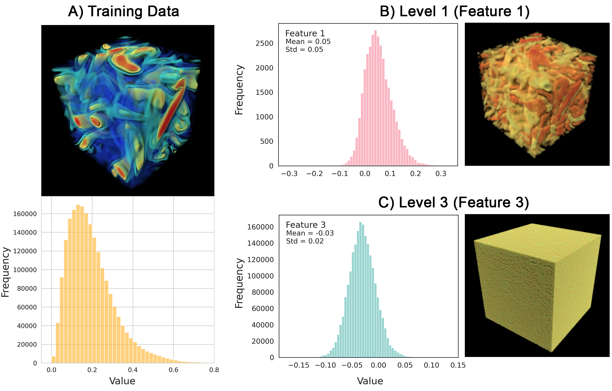
Figure 5: A) The volume visualization of the vortices data as well as the histogram data values. B), C) Volume visualizations and histograms of the corresponding hash encoding weights.

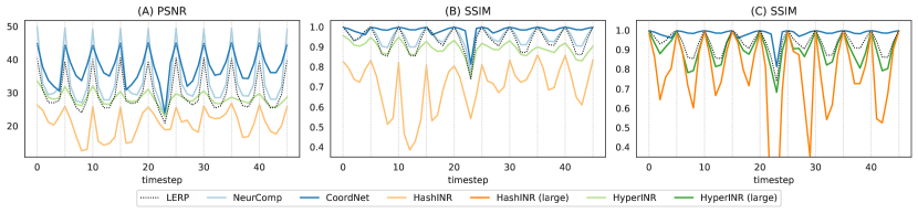
Figure 6: Comparisons of different INR architectures on the temporal super-resolution task. A), B) Comparisons of networks with equalized number of trainable parameters. C) To rule out the possibility that HashINR and HyperINR were limited by network capacity, another comparison were performed against a HashINR with a very large hash table size ($T=2^{21}$) and a HyperINR with sufficient hash encoders ($N=24$).

5 Ablation Study

In this section, we present results and findings that motivate the design of HyperINR, and conduct a hyperparameter study to determine the optimal configuration for our tasks.

5.1 Understand Hash Encoding Weights

Designing an accurate hypernetwork for predicting multiresolution hash encoding weights requires a thorough understanding of these weights. To gain insight, we mapped the weights of each encoding level back to the corresponding grid space $\{\leavevmode\nobreak\ g_{x,y,z}=W_{\text{hash}(x,y,z)}\leavevmode\nobreak\ \}$, and visualized them using histograms and volume renderings, as shown in Figure 5.

Parametric Encoding is an Embedding of Local Features

Our analysis reveals that when the number of grid vertices is smaller than the hash table size, a strong correlation exists between the encoder parameter values and the actual data values. Furthermore, different features tend to capture different details, resulting in distinct weight distributions. These observations suggest that INRs with parametric encoding operate differently from those parameterized solely by MLPs. With parametric encoding, local details in the data are simply projected into a high-dimensional weight space, rather than being approximated indirectly through MLPs. These findings agree with our intuition about parametric encoding and explain why employing multiresolution hash encoding can result in a loss of generalizability.

Hash Function Breaks Local Similarities

When the total number of grid vertices exceeds the hash table size, a spatial hash function is utilized to condense encoding parameters. Our results indicate that this process breaks the aforementioned correlation between parameter values and data values. These local similarities are broken in the hashed space and cannot be restored. This suggests that when designing a hypernetwork for multiresolution hash encoding, levels processed by the spatial hash function must be treated differently from those without it. Operations such as CNNs that take advantage of local spatial coherence may not work even after remapping encoding parameters back to the grid space. Our findings motivate us to focus on weight interpolation methods that rely solely on correlations between parameters stored at the same location in the hash table.

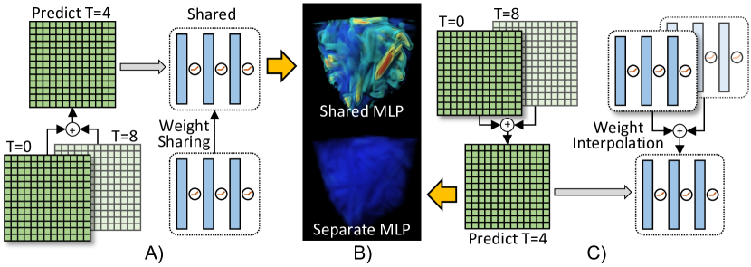
Figure 7: Comparisons of different weight interpolation methods. A) The method that uses a shared MLP. B) Volume rendering results. C) The naïve design that employs different MLPs for different hash encoders.

5.2 Shared MLP Unit

The fundamental principle behind HyperINR is the effective organization of the INR weight space to facilitate interpolation. Thus, it is crucial to first identify the appropriate interpolation method. In this section, we examine two weight interpolation designs. These two designs are visually illustrated in Figure 7.

The straightforward design involves optimizing a standalone INR for each training data, and then interpolating all the network weights for parameters outside the training set. However, this design demonstrates a lack of robustness to perturbations (i.e., different random seedings), resulting in totally different network weights if repeatedly trained on the same dataset. While these INRs can yield similar inference outcomes, interpolating among their network weights is generally meaningless because network parameters in the same relative location may hold entirely different meanings across INR instances. The lower part of Figure 7B presents a volume rendering result of the INR produced by this weight interpolation design.

In contrast, we construct our HyperINR by incorporating a shared MLP among all positional encoders. This MLP serves as a common projector, ensuring consistent meanings for network parameters across different INR instances and thus rendering weight interpolation feasible. Our finding, depicted in the upper part of Figure 7B, substantiates the effectiveness of a shared MLP unit in enabling meaningful weight interpolation for HyperINR.

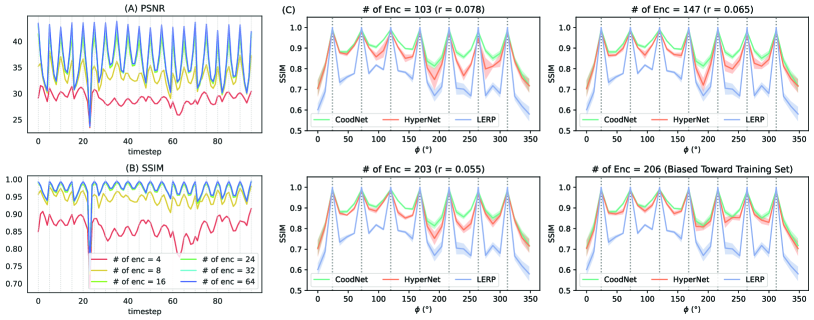
Figure 8: The impact of hash encoder positions $\mathcal{E}$ on the data reconstruction quality was examined in two tasks. The first task, A-B), conducted temporal super-resolution using the vortices dataset. The second task, C), used the mechhand dataset to address dynamic global shadows. In C), each line represents the average SSIM across 5 different $\theta$ angles, with filled areas highlighting the $\pm$ 1 standard deviation regions.

5.3 Comparison between INRs

With a good interpolation strategy, we now investigate the necessity of employing a hypernetwork to achieve both good generalizability and inference speed. In this section, we present experimental comparison between HyperINR and three distinct INR architectures. We conducted our experiments on the TSR task, utilizing the vortices dataset.

The three neural networks we employed in our experiment are CoordNet [14], NeurComp [23], and a hash encoding based INR extended to 4 dimensions (HashINR). We included CoordNet and NeurComp in our experiment as CoordNet has recently demonstrated strong performance on TSR tasks, and there is no report of NeurComp on TSR tasks to the best of our knowledge. HashINR processes spatial coordinates using hash encoding and time using OneBlob encoding [29]. Such a HashINR has been used by several computer graphics works [30] and demonstrated good learning capabilities while offering very good inference performance.

To ensure fair comparisons, we used the standard CoordNet configuration described in Section 4 and equalized the number of trainable parameters used in all the other networks (to around 2.1$\sim$2.2M). Specifically, for NeurComp, we used 10 resblocks of size 327; for HyperINR, we constructed 6 small hash encoders ($T=2^{14}$); and for HashINR, we used medium-sized hash tables ($T=2^{17}$). We optimized all the networks sufficiently and report their performances in Figure 6A-B. Notably, we observed that HashINR did not perform well. To rule out the possibility that the HashINR was limited by its network capacity, we performed another comparison against a HashINR with very large hash tables ($T=2^{21}$) and a HyperINR with sufficient hash encoders ($N=24$), with results highlighted in Figure 6C.

Our experimental results lead us to three conclusions. Firstly, under equal conditions, CoordNet performed significantly better than NeurComp in terms of generalizability. This is likely due to the differences in network design, as their network capacities were equalized. Secondly, compared with two pure MLP-based INRs, HashINR was unable to achieve good performance using the same amount of trainable parameters. Even after increasing the hash table size, HashINR still struggled to perform well on unseen parameters. Finally, we found that HyperINR outperformed HashINR in terms of generalizability by splitting a larger hash table into multiple smaller ones. However, there was still a performance gap compared to CoordNet. To bridge this gap, we utilize knowledge distillation.

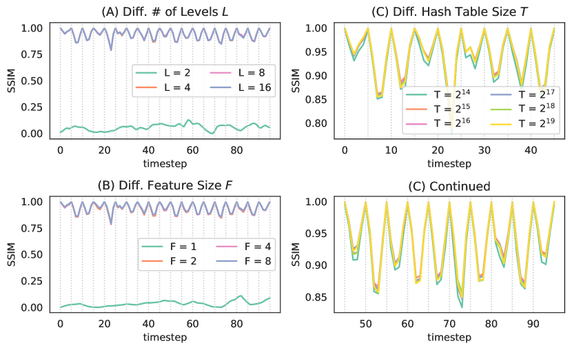
Figure 9: Hyperparameter study of hash encoder parameters.

5.4 Hyperparameter Study

With a strong network architecture, we now determine the optimal hyperparameters for HyperINR. Specifically, we examined parameters related to individual hash encoders, as well as the impact of encoder positions in the parameter space on performance.

Hash Encoder Parameters

To evaluate parameters related to individual hash encoders, we constructed various HyperINRs and tasked them with performing TSR on the vortices dataset. We maintained a fixed number of 24 encoders, distributed uniformly throughout the temporal domain, and assessed reconstruction quality using SSIM. Results are reported in Figure 9.

First, we set $T=2^{15}$, $F=4$, and varied the number of encoding levels $L$ from 1 to 16. Our findings suggest that $L>2$ is sufficient for this particular TSR problem. Increasing $L$ does not yield significant improvements in generalizability. Next, we held $L$ constant at 8 and varied the number of features per encoding level $F$ from 1 to 8. Results showed that good performance can be achieved with $F>1$, but increasing $F$ yields diminishing returns. Finally, with $F=4$ held constant, we adjusted the hash table size $T$ from $2^{14}$ to $2^{19}$. In general, we observed that a larger hash table size leads to better reconstruction quality, although the differences were minimal for our particular problem.

We conclude that selecting appropriate hyperparameters depends on the data complexity, and for more complicated data, larger hyperparameter values are likely necessary. We repeated these experiments using other datasets and determined that $T=2^{15}$, $F=4$, and $L=8$ generally produce good performance across all cases considered in this study.

Hash Encoder Locations

In this section, we present our investigation of the impact of hash encoder positions $\mathcal{E}$ on data prediction quality. We began by studying the problem in 1D using the TSR task and subsequently move to higher dimensions using the DGS task.

For the TSR task, we utilized the vortices dataset and construct 6 HyperINR networks with varying numbers of hash encoders, as depicted in Figure 8AB. These hash encoders were uniformly distributed along the time axis and configured equally based on findings obtained from the experiment described in Section 5.4. We then followed our knowledge distillation process, utilizing a pre-trained CoordNet to distill all the HyperINRs equally and sufficiently (i.e., more than 30k epochs). Network performances were measured using PSNR and SSIM. Our results show that the knowledge of a CoordNet can be fully distilled into a HyperINR with 16 or more hash encoders. Notably, this number is close to the number of training samples in the TSR task. Further experimentation on the pressure and temperature datasets confirms that this is not a coincidence. We conclude that, for TSR tasks, the number of hash encoders needs to be comparable to the training set size to ensure good knowledge distillation performance.

Moving to higher dimensions, we conducted experiments using the DGS task with 4 different HyperINRs. For the first three networks, we used Poisson disk sampling to generate encoder positions $\mathcal{E}$ with different disk radii, resulting in approximately 100, 150, and 200 hash encoders, as shown in Figure 8C. For the fourth model, we used approximately 200 hash encoders, but with 3/4 of them positioned using Gaussian kernels centered around training set parameters. This resulted in a stronger bias towards the training data. Our results, as shown in Figure 8C, demonstrate that our model can significantly outperform direct data interpolation with only 100 hash encoders. But this amount of hash encoders cannot fully capture CoordNet’s behavior. Nevertheless, gradually adding more hash encoders can shrink the gap between CoordNet and HyperINR, indicating that Poisson disk sampling in general can provide a good heuristic for hash encoder positions. Moreover, it is possible to further improve the model’s performance and allow it to be biased towards known information. This operation can be useful if there is prior knowledge about which areas of the parameter space will be explored more.

6 Application Performance

This section presents the performance of HyperINR in terms of prediction quality and inference speed for each application. We provide a summary of the training-related information in Table 2.

Table 2: Training results measured using a single NVIDIA A100-40G GPU. Teacher models were trained for 30k (TSR, DGS) or 300 (NVS) epochs. Distillations were performed for 5k (TSR, DGS) or 200 (NVS) epochs. The distillation time for temp and mechhand were significantly longer because their distillation sets were larger than the GPU memory capacity, pushing a lot of data to the CPU, causing the training process to be bottlenecked by the GPU/CPU bandwidth.

Data	Task	$T_{\text{teacher}}$	$T_{\text{distill}}$	$N_{C}$	$N_{D}$	Generation Latency
Vortices	TSR	1h04m	19m	20	100	0.08ms
Pressure	TSR	1h21m	20m	20	105	0.07ms
Temp	TSR	36m	3h34m	10	100	0.07ms
MPAS	NVS	54m	23m	100	981	0.27ms
MechHand	DGS	1h47m	4h09m	35	400	0.28ms

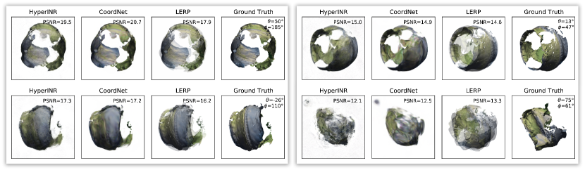
Figure 10: Results for the novel view synthesis task performed on the MPAS dataset. The dataset was created by He et al. [17]. Compared with CoordNet, HyperINR can instantaneously generate novel views while maintaining similar qualities.

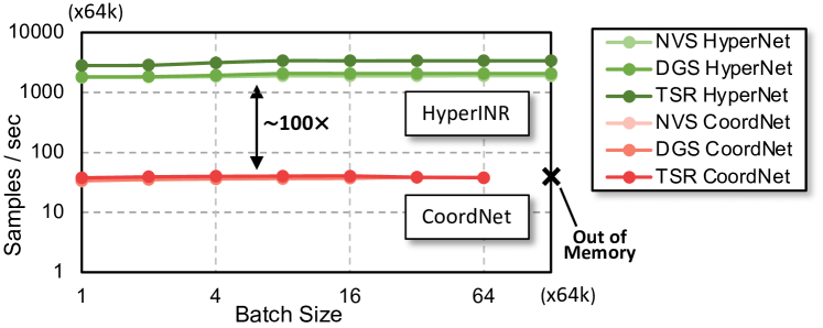
Figure 11: Network inference bandwidth comparisons between CoordNet and HyperINR. Measured using a single NVIDIA A100-40G GPU.

6.1 Novel View Synthesis

To evaluate the image generation quality of HyperINR, we predicted images for all parameters in the evaluation set using HyperINR and inverse distance weighting (LERP), and compared them with the actual images in the evaluation set. We then calculated the PSNR scores and highlight the differences in Figure 12. Our visualizations show that HyperINR-generated images generally have higher PSNR scores compared to LERP-generated images. We also conducted a statistical hypothesis test on whether the PSNR differences were statistically greater than zero. The p-value for the test was $1.2\times 10^{-12}<0.05$, indicating a significant difference.

The predicted images are displayed in Figure 10, which also includes results generated by CoordNet for comparison. We found that CoordNet could generally predict images at novel views well, while LERP images would produce distracting artifacts. HyperINR could avoid these artifacts but introduced some high-frequency noises. Despite these advantages, we observed that when CoordNet’s performance was not satisfactory, HyperINR’s performance also deteriorated, highlighting one of the limitations of our approach. Finally, we compared the network inference throughput between CoordNet and HyperINR in Figure 11 and found that our method was around $100\times$ faster.

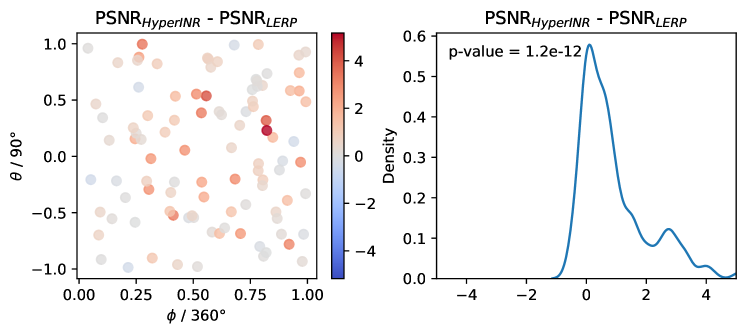
Figure 12: Visualizations of the PSNR differences between HyperINR and LERP on the MPAS evaluation set. Left: the scatter plot highlighting the sample location in the parameter space. We encode the PSNR differences as marker colors. Right: the kernel density estimation of the PSNR differences. Additionally, a statistical test (one-sample t-test) was performed to verify if the PSNR differences were positive.

6.2 Temporal Super Resolution

We performed TSR tasks using three datasets and evaluated CoordNet, HyperINR, and LERP at all timesteps, calculating the PSNRs and SSIMs with respect to the ground truths, shown in Figure 13. We also display volumetric path tracing results of selected timesteps in HyperINR: A Fast and Predictive Hypernetwork for Implicit Neural Representations via Knowledge Distillation and Figure 14 for all datasets.

Our visualizations show that HyperINR was able to closely match the performance of CoordNet for all the datasets. Based on our volume rendering results, we found that HyperINR-generated results were generally more structurally accurate compared to LERP-generated results. However, HyperINR failed to outperform LERP on datasets that were intrinsically suitable for interpolation, such as the pressure dataset shown in Figure 13A. For datasets containing many fine details like the temperature dataset shown in Figure 13B, HyperINR’s results were more accurate in terms of PSNR and SSIM, but high-frequency details were mostly missing on rendered images. LERP was able to generate data containing many details, but these details were inaccurate.

In terms of performance, we found that HyperINR achieved good volume rendering performance (20$\sim$30fps). Note that these results were rendered using a costly volumetric path tracing algorithm with one directional light. The same framesize (800$\times$600), samples per pixels (spp = 1) and lighting configuration (1 directional light) were used for all the experiments. Additionally, model inference bandwidths were also measured and presented in Figure 11.

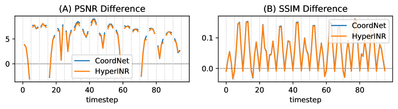
Figure 13: Comparisons of the network reconstruction quality between HyperINR and CoordNet for the temporal super-resolution task, performed on the vortices dataset.

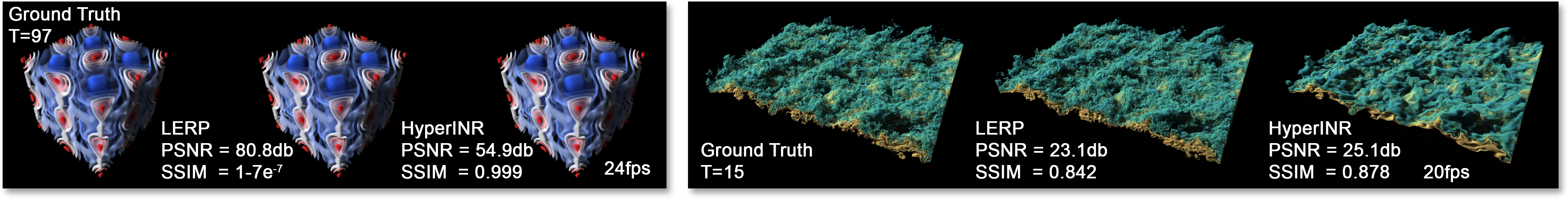
Figure 14: Rendering results of temporal super-resolution experiments using (Left) the pressure dataset and (Right) the temperature dataset. Renderings were performed on a single NVIDIA RTX8000 GPU.

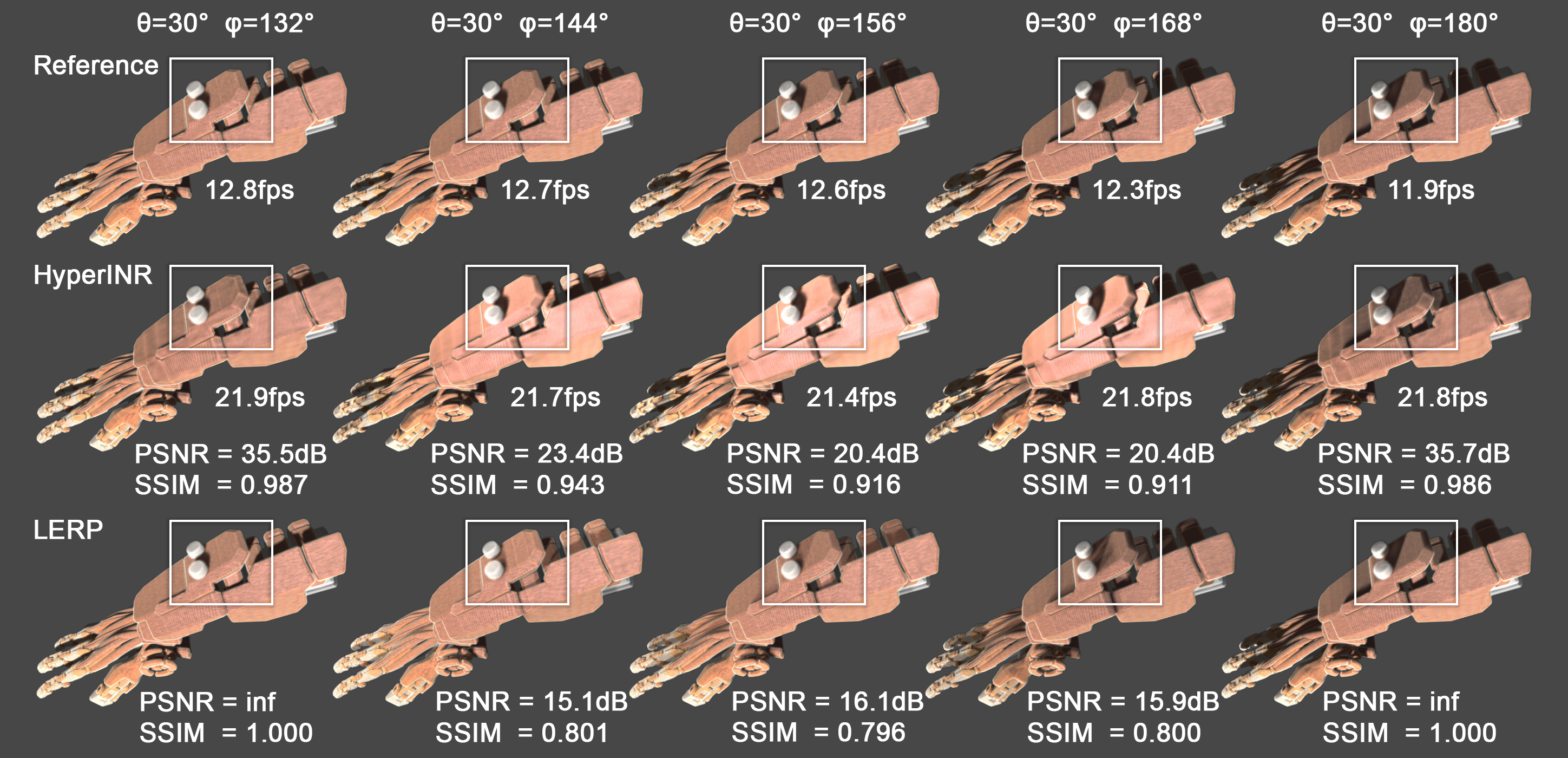
Figure 15: Rendering results of the dynamic global shadow task. Renderings were performed on a single NVIDIA RTX8000 GPU. As highlighted by white boxes, HyperINR could more accurately predict the shadow movements, while LERP gradually faded shadows in and out.

6.3 Dynamic Global Shadow

For the DGS task, we used an INR to encode shadow coefficients and created global shadows for the MechHand dataset. We have already highlighted the PSNR and SSIM results of this experiment in Section 5.4. Here, we focus on the visual quality aspect.

In Figure 15, we compared global shadows generated using secondary rays (i.e., the reference), HyperINR, and LERP. We gradually adjusted the azimuthal angle $\phi$ from 132^∘ to 180^∘ while fixing the polar angle $\theta$. The first and last data frames were presented in the training set. Our visualizations show that LERP could not correctly predict the movement of the shadow and gradually faded shadows in and out. Conversely, HyperINR was able to plausibly predict the shadow movement. However, the generated INR seemed to also make the volume brighter in some areas, perhaps due to some incorrectly predicted shadow coefficient values.

Additionally, we highlight the rendering performance differences in Figure 15. We found that our method significantly improved the rendering performance by avoiding secondary rays. For the tested configuration, we observed a roughly $2\times$ speedup. Furthermore, we present the INR generation latency in Table 2, which indicates that our method can support real-time shadow INR generations.

7 Discussion and Future Work

In this section, we present four key insights derived from our study.

Firstly, our results generally highlight HyperINR’s exceptional performance for data and visualization generation. This can be attributed to the incorporation of CoordNet, which is a highly effective teacher network. In addition, our experiments also demonstrate the possibility to construct a hypernetwork with a weight space meaningful for interpolation. Such a hypernetwork can continuously approximate a high-dimensional space utilizing a finite number of encoder instances. Although we employ knowledge distillation for optimization in this study, directly optimizing a generative hypernetwork to achieve comparable data generation performance should be feasible and represents a promising research direction.

Secondly, our HyperINR leverages numerous small multiresolution hash encoders to approximate data modeled by high-dimensional parameters, providing a more flexible and effective approach compared to using a single large encoder. This observation is corroborated by our ablation study, as detailed in Section 5.3. This attribute makes HyperINR well-suited for learning ensembles of data comprising diverse data frames. Nonetheless, as highlighted in Section 5.4, efficiently constructing encoder positions can be challenging and often necessitates extensive experimentation. In higher dimensions, the addition of encoders does not always result in a linear improvement in HyperINR’s performance. Therefore, a more general and effective method for computing encoder positions is highly desirable.

Thirdly, as demonstrated in Table 2, knowledge distillation employed to train HyperINR can be time-consuming due to two factors. For one, achieving high distillation quality may require a large distillation set, prolonging the training process. Secondly, when the distillation set is generated on-demand, the training speed can be significantly constrained by the inference bandwidth of CoordNet. We alleviated this bottleneck by pre-computing the distillation set, resulting in up to an $8\times$ speedup on an NVIDIA A100 for certain cases. However, this optimization remains inefficient when the distillation set size surpasses the GPU memory capacity, pushing training data to the CPU and causing the training process to be constricted by the CPU/GPU bandwidth. Exploring more effective distillation set generation methods warrants further investigation.

Lastly, while knowledge distillation can substantially enhance HyperINR’s data generation capabilities, it also imposes an upper limit on its performance. In cases where the teacher network underperforms, HyperINR’s performance may also be considerably hindered, as illustrated in Figure 14. Investigating more flexible training strategies represents a promising avenue for future research.

8 Conclusion

We introduce HyperINR, an innovative hypernetwork facilitating conditional generation of INRs for unseen scene parameters. Enabled by the employment of numerous small multiresolution hash encoders, a shared MLP, and a deeply embedded weight interpolation operation, HyperINR achieves an impressive $100\times$ higher inference bandwidth and interactive volume rendering with exceptional realism. Moreover, our method attains state-of-the-art data and visualization generation performance through knowledge distillation. Our results underscore the potential of HyperINR in various visualization tasks, showcasing its effectiveness and efficiency. We believe that HyperINR represents a step forward in the development of implicit neural representation based approaches for the field of scientific visualization and beyond.

- [1] J. T. Barron, B. Mildenhall, M. Tancik, P. Hedman, R. Martin-Brualla, and P. P. Srinivasan. Mip-NeRF: A multiscale representation for anti-aliasing neural radiance fields. In Proceedings of the IEEE/CVF International Conference on Computer Vision, pp. 5855–5864, 2021.
- [2] D. Bauer, Q. Wu, and K.-L. Ma. Fovolnet: Fast volume rendering using foveated deep neural networks. IEEE Transactions on Visualization and Computer Graphics, 29(1):515–525, 2023. doi: 10 . 1109/TVCG . 2022 . 3209498
- [3] M. Berger, J. Li, and J. A. Levine. A generative model for volume rendering. IEEE transactions on visualization and computer graphics, 25(4):1636–1650, 2018.
- [4] L. Bertinetto, J. F. Henriques, J. Valmadre, P. Torr, and A. Vedaldi. Learning feed-forward one-shot learners. Advances in neural information processing systems, 29, 2016.
- [5] R. Bridson. Fast poisson disk sampling in arbitrary dimensions. SIGGRAPH sketches, 10(1):1, 2007.
- [6] C. Buciluă, R. Caruana, and A. Niculescu-Mizil. Model compression. In Proceedings of the 12th ACM SIGKDD international conference on Knowledge discovery and data mining, pp. 535–541, 2006.
- [7] D. Engel and T. Ropinski. Deep volumetric ambient occlusion. IEEE Transactions on Visualization and Computer Graphics, 27(2):1268–1278, 2020.
- [8] J. Gehring, M. Auli, D. Grangier, D. Yarats, and Y. N. Dauphin. Convolutional sequence to sequence learning. In International Conference on Machine Learning, pp. 1243–1252. PMLR, 2017.
- [9] L. Guo, S. Ye, J. Han, H. Zheng, H. Gao, D. Z. Chen, J.-X. Wang, and C. Wang. SSR-VFD: Spatial super-resolution for vector field data analysis and visualization. In Proceedings of IEEE Pacific Visualization Symposium, 2020.
- [10] D. Ha, A. Dai, and Q. V. Le. Hypernetworks. arXiv preprint arXiv:1609.09106, 2016.
- [11] S. Hadadan, S. Chen, and M. Zwicker. Neural radiosity. ACM Transactions on Graphics (TOG), 40(6):1–11, 2021.
- [12] J. Han and C. Wang. TSR-TVD: Temporal super-resolution for time-varying data analysis and visualization. IEEE transactions on visualization and computer graphics, 26(1):205–215, 2019.
- [13] J. Han and C. Wang. SSR-TVD: Spatial super-resolution for time-varying data analysis and visualization. IEEE Transactions on Visualization and Computer Graphics, 2020.
- [14] J. Han and C. Wang. Coordnet: Data generation and visualization generation for time-varying volumes via a coordinate-based neural network. IEEE Transactions on Visualization and Computer Graphics, 2022.
- [15] J. Han and C. Wang. Vcnet: A generative model for volume completion. Visual Informatics, 6(2):62–73, 2022.
- [16] J. Han, H. Zheng, D. Z. Chen, and C. Wang. STNet: An end-to-end generative framework for synthesizing spatiotemporal super-resolution volumes. IEEE Transactions on Visualization and Computer Graphics, 28(1):270–280, 2021.
- [17] W. He, J. Wang, H. Guo, K.-C. Wang, H.-W. Shen, M. Raj, Y. S. Nashed, and T. Peterka. Insitunet: Deep image synthesis for parameter space exploration of ensemble simulations. IEEE transactions on visualization and computer graphics, 26(1):23–33, 2019.
- [18] G. Hinton, O. Vinyals, and J. Dean. Distilling the knowledge in a neural network. arXiv preprint arXiv:1503.02531, 2015.
- [19] S. Jain, W. Griffin, A. Godil, J. W. Bullard, J. Terrill, and A. Varshney. Compressed volume rendering using deep learning. In Proceedings of the Large Scale Data Analysis and Visualization (LDAV) Symposium. Phoenix, AZ, 2017.
- [20] D. Kim, M. Lee, and K. Museth. Neuralvdb: High-resolution sparse volume representation using hierarchical neural networks. arXiv preprint arXiv:2208.04448, 2022.
- [21] S. Klocek, Ł. Maziarka, M. Wołczyk, J. Tabor, J. Nowak, and M. Śmieja. Hypernetwork functional image representation. In Artificial Neural Networks and Machine Learning–ICANN 2019: Workshop and Special Sessions: 28th International Conference on Artificial Neural Networks, Munich, Germany, September 17–19, 2019, Proceedings 28, pp. 496–510. Springer, 2019.
- [22] G. Littwin and L. Wolf. Deep meta functionals for shape representation. In Proceedings of the IEEE/CVF International Conference on Computer Vision, pp. 1824–1833, 2019.
- [23] Y. Lu, K. Jiang, J. A. Levine, and M. Berger. Compressive neural representations of volumetric scalar fields. vol. 40, pp. 135–146, 2021. doi: 10 . 1111/cgf . 14295
- [24] J. N. Martel, D. B. Lindell, C. Z. Lin, E. R. Chan, M. Monteiro, and G. Wetzstein. Acorn: Adaptive coordinate networks for neural scene representation. arXiv preprint arXiv:2105.02788, 2021.
- [25] P. Micikevicius, S. Narang, J. Alben, G. Diamos, E. Elsen, D. Garcia, B. Ginsburg, M. Houston, O. Kuchaiev, G. Venkatesh, et al. Mixed precision training. arXiv preprint arXiv:1710.03740, 2017.
- [26] B. Mildenhall, P. P. Srinivasan, M. Tancik, J. T. Barron, R. Ramamoorthi, and R. Ng. Nerf: Representing scenes as neural radiance fields for view synthesis. In European conference on computer vision, pp. 405–421. Springer, 2020.
- [27] T. Müller. Tiny CUDA neural network framework, 2021 (Online). https://github.com/nvlabs/tiny-cuda-nn.
- [28] T. Müller, A. Evans, C. Schied, and A. Keller. Instant neural graphics primitives with a multiresolution hash encoding. ACM Transactions on Graphics (ToG), 41(4):1–15, 2022.
- [29] T. Müller, B. McWilliams, F. Rousselle, M. Gross, and J. Novák. Neural importance sampling. ACM Transactions on Graphics (TOG), 38(5):1–19, 2019.
- [30] T. Müller, F. Rousselle, J. Novák, and A. Keller. Real-time neural radiance caching for path tracing. arXiv preprint arXiv:2106.12372, 2021.
- [31] P. Nguyen, T. Tran, S. Gupta, S. Rana, H.-C. Dam, and S. Venkatesh. Hypervae: A minimum description length variational hyper-encoding network. CoRR, 2020.
- [32] G. Oh and J.-S. Valois. Hcnaf: Hyper-conditioned neural autoregressive flow and its application for probabilistic occupancy map forecasting. In Proceedings of the IEEE/CVF Conference on Computer Vision and Pattern Recognition, pp. 14550–14559, 2020.
- [33] N. Ratzlaff and L. Fuxin. Hypergan: A generative model for diverse, performant neural networks. In International Conference on Machine Learning, pp. 5361–5369. PMLR, 2019.
- [34] M. Rieth, A. Gruber, F. A. Williams, and J. H. Chen. Enhanced burning rates in hydrogen-enriched turbulent premixed flames by diffusion of molecular and atomic hydrogen. Combustion and Flame, p. 111740, 2021.
- [35] D. Shepard. A two-dimensional interpolation function for irregularly-spaced data. In Proceedings of the 1968 23rd ACM national conference, pp. 517–524, 1968.
- [36] N. Shi, J. Xu, H. Li, H. Guo, J. Woodring, and H.-W. Shen. Vdl-surrogate: A view-dependent latent-based model for parameter space exploration of ensemble simulations. IEEE Transactions on Visualization and Computer Graphics, 29(1):820–830, 2022.
- [37] V. Sitzmann, J. N. Martel, A. W. Bergman, D. B. Lindell, and G. Wetzstein. Implicit neural representations with periodic activation functions. In arXiv, 2020.
- [38] V. Sitzmann, M. Zollhöfer, and G. Wetzstein. Scene representation networks: Continuous 3d-structure-aware neural scene representations. Advances in Neural Information Processing Systems, 32, 2019.
- [39] I. Skorokhodov, S. Ignatyev, and M. Elhoseiny. Adversarial generation of continuous images. In Proceedings of the IEEE/CVF Conference on Computer Vision and Pattern Recognition, pp. 10753–10764, 2021.
- [40] T. Takikawa, J. Litalien, K. Yin, K. Kreis, C. Loop, D. Nowrouzezahrai, A. Jacobson, M. McGuire, and S. Fidler. Neural geometric level of detail: Real-time rendering with implicit 3d shapes. In Proceedings of the IEEE/CVF Conference on Computer Vision and Pattern Recognition, pp. 11358–11367, 2021.
- [41] M. Tancik, P. Srinivasan, B. Mildenhall, S. Fridovich-Keil, N. Raghavan, U. Singhal, R. Ramamoorthi, J. Barron, and R. Ng. Fourier features let networks learn high frequency functions in low dimensional domains. Advances in Neural Information Processing Systems, 33:7537–7547, 2020.
- [42] A. Tikhonova, C. D. Correa, and K.-L. Ma. Explorable images for visualizing volume data. PacificVis, 10:177–184, 2010.
- [43] A. Vaswani, N. Shazeer, N. Parmar, J. Uszkoreit, L. Jones, A. N. Gomez, Ł. Kaiser, and I. Polosukhin. Attention is all you need. Advances in neural information processing systems, 30, 2017.
- [44] J. Von Oswald, C. Henning, J. Sacramento, and B. F. Grewe. Continual learning with hypernetworks. arXiv preprint arXiv:1906.00695, 2019.
- [45] C. Wang and J. Han. Dl4scivis: A state-of-the-art survey on deep learning for scientific visualization. IEEE Transactions on Visualization and Computer Graphics, 2022.
- [46] S. Weiss, M. Chu, N. Thuerey, and R. Westermann. Volumetric isosurface rendering with deep learning-based super-resolution. IEEE transactions on visualization and computer graphics, 27(6):3064–3078, 2019.
- [47] S. Weiss, P. Hermüller, and R. Westermann. Fast neural representations for direct volume rendering. Computer Graphics Forum, 41(6):196–211, 2022. doi: 10 . 1111/cgf . 14578
- [48] Q. Wu, D. Bauer, M. J. Doyle, and K.-L. Ma. Instant neural representation for interactive volume rendering. arXiv preprint arXiv:2207.11620, 2022.
- [49] S. W. Wurster, H.-W. Shen, H. Guo, T. Peterka, M. Raj, and J. Xu. Deep hierarchical super-resolution for scientific data reduction and visualization. arXiv preprint arXiv:2107.00462, 2021.
- [50] C. Zhang, M. Ren, and R. Urtasun. Graph hypernetworks for neural architecture search. arXiv preprint arXiv:1810.05749, 2018.
- [51] Z. Zhou, Y. Hou, Q. Wang, G. Chen, J. Lu, Y. Tao, and H. Lin. Volume upscaling with convolutional neural networks. In Proceedings of the Computer Graphics International Conference, pp. 1–6, 2017.