Interferometry of multi-level systems: rate-equation approach for a charge qudit

Abstract

We theoretically describe a driven two-electron four-level double-quantum dot (DQD) tunnel coupled to a fermionic sea by using the rate-equation formalism. This approach allows to find occupation probabilities of each DQD energy level in a relatively simple way, compared to other methods. Calculated dependencies are compared with the experimental results. The system under study is irradiated by a strong driving signal and as a result, one can observe Landau-Zener-Stückelberg-Majorana (LZSM) interferometry patterns which are successfully described by the considered formalism. The system operation regime depends on the amplitude of the excitation signal and the energy detuning, therefore, one can transfer the system to the necessary quantum state in the most efficient way by setting these parameters. Obtained results give insights about initializing, characterizing, and controlling the quantum system states.

I Introduction

Fast development of the quantum computing field requires sophisticated practical solutions. One of such solutions are quantum dots. These systems are good candidates for being building blocks of quantum computers, since they have good tunability [Veldhorst et al., 2014] and flexible coupling geometry [Shulman et al., 2012]. Also, quantum dots demonstrate good performance for readout, manipulation, and initialization of their spin states [Petta et al., 2005; Hanson et al., 2005; Kiyama et al., 2016; Friesen et al., 2004]. Such systems can be used for quantum information [Cerletti et al., 2005, Loss and DiVincenzo, 1998] and quantum computing [DiVincenzo et al., 2000; Byrd and Lidar, 2002]. Considered objects are also interesting for studying quantum luminescence [Kim, 1998; Romero and van de Lagemaat, 2009], superconductivity [Estrada Saldaña et al., 2018], Kondo effect [Sasaki et al., 2004], solid-state energy conversion [Beenakker and Staring, 1992], quantum communication [Simon et al., 2007; Huwer et al., 2017], piezomagnetic effect [Abolfath et al., 2008], etc.

For solving many modern problems (one of them is a creation of a quantum computer), it is not enough to use a single quantum dot, thus one should connect them into chains [Flentje et al., 2017]. The behavior of electrons in a chain can be decomposed on interactions between pairs of adjacent dots, called double quantum dots (DQDs). As a result these systems are widely explored nowadays. Particularly, it was stressed that DQDs open opportunities for probing electron-phonon coupling [Brandes, 2005], allow to probe the semiconductor environment [van der Wiel et al., 2002], can be used in the relatively new and promising area of spintronics [Awschalom and Flatte, 2007], serve as thermoelectric generators [Donsa et al., 2014] and noise detectors [Aguado and Kouwenhoven, 2000]. Therefore, both experimental and theoretical study of such systems is very important not only from quantum information point of view but also for modern quantum physics in general.

In the current paper we theoretically study the properties of a qudit (d-level quantum system) [Liu et al., 2017; Wang et al., 2020; Han et al., 2019; Kononenko et al., 2021; Yurtalan et al., 2020] similar to the one experimentally studied in Ref. [Chatterjee et al., 2018]. The main tool of our analysis is the rate-equation formalism [Ferrón et al., 2012, 2016; Liul and Shevchenko, 2023], which is relatively simple, but often shows good agreement with experiments. For example, this method successfully describes the behavior of a two-level system [Berns et al., 2006] as well as a multi-level system (solid-state artificial atom) from Ref. [Oliver and Valenzuela, 2009] which was analyzed in Ref. [Wen and Yu, 2009].

Present research could also be interesting since it opens an additional opportunity for studying the Landau-Zener-Stückelberg-Majorana (LZSM) transitions. This effect can be observed if one irradiates a quantum system by a signal with the frequency which is much smaller than the distance between energy levels [Izmalkov et al., 2004; Ashhab, 2014]. LZSM transitions appear in many fields; for instance, in solid-state physics [Nakonechnyi et al., 2021; Liul et al., 2023], quantum information science [Fuchs et al., 2011; Ribeiro and Burkard, 2009], nuclear physics [Thiel, 1990], chemical physics [Zhu et al., 1997], and quantum optics [Bouwmeester et al., 1995]. Repeated LZSM transitions result in LZSM interference [Stehlik et al., 2012; Oliver et al., 2005; Gonzalez-Zalba et al., 2016; Kofman et al., 2023; Ono et al., 2019]. The LZSM interferometry can be used for a quantum system description and control [Wu et al., 2019; Ivakhnenko et al., 2023]; it allows to understand better processes of photon-assisted transport in superconducting systems [Nakamura and Tsai, 1999] and decoherence in quantum systems [Rudner et al., 2008; Malla and Raikh, 2022].

The rest of the paper is organized as follows. In Sec. II the rate-equation formalism for a TLS is laid out with its subsequent generalization on multi-level systems. The considered model is applied for the analysis of the two-electron double quantum dot in Sec. III. Section IV is devoted to a DQD studied in the three-level approximation. In Sec. V we present our conclusions. The expressions for building DQD energy levels diagram are presented in Appendix A.

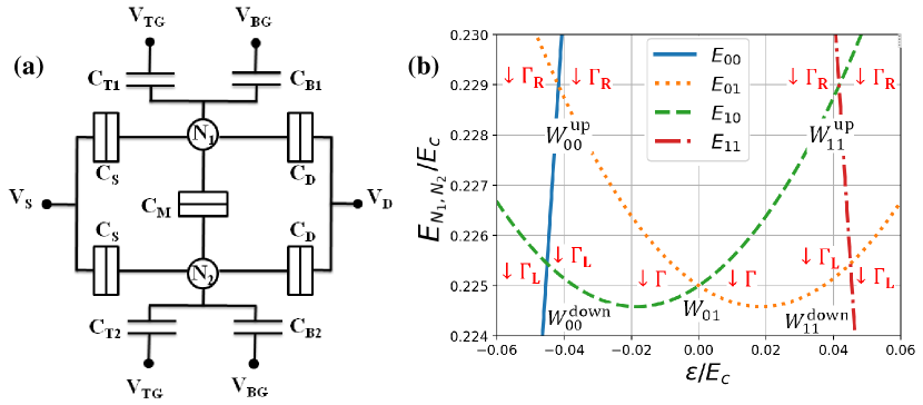
Figure 1: Scheme of the DQD and its energy levels in the charge basis. Panel (a) shows the electrical scheme of the considered DQD, with $N_{1}$ and $N_{2}$ being the numbers of electrons in each dot, $V$ and $C$ with the subscripts indicate the respective applied voltages and capacitances. (b) Energy levels of the DQD similar to the one studied in Ref. [Chatterjee et al., 2018] in the charge basis. The expression for the electrostatic energy $E_{N_{1},N_{2}}$ is given by Eq. (23), the characteristic charging energy $E_{C}$ is defined after Eq. (23). The values $W_{00}^{\rm up}$ and $W_{00}^{\rm down}$ are the transition rates between the state $\left|00\right\rangle$ and the states $\left|01\right\rangle$, $\left|10\right\rangle$, respectively. The values $W_{11}^{\rm up}$ and $W_{11}^{\rm down}$ are the transition rates between the state $\left|11\right\rangle$ and the states $\left|10\right\rangle$, $\left|01\right\rangle$, respectively. The transition rate $W_{01}$ indicates transitions between the states $\left|01\right\rangle$ and $\left|10\right\rangle$. The value $\Gamma_{\rm L}$ is the relaxation rate between the states $\left|00\right\rangle$ and $\left|10\right\rangle$, $\left|11\right\rangle$ and $\left|01\right\rangle$ (left dot and reservoirs in terms of the experiment). The value $\Gamma_{\rm R}$ is the relaxation rate between the states $\left|00\right\rangle$ and $\left|01\right\rangle$, $\left|11\right\rangle$ and $\left|10\right\rangle$ (right dot and reservoirs in terms of the experiment), $\Gamma$ is the relaxation rate between states $\left|01\right\rangle$ and $\left|10\right\rangle$.

II Rate-equation approach

In this section, we describe theoretical aspects of the rate-equation formalism. For doing this, we first employ this method for a two-level system with further extension of obtained results on multi-level systems. The Hamiltonian of a TLS driven by an external field can be written in the form

$$\widehat{H}(t)=-\frac{\mathrm{\Delta}}{2}\widehat{\sigma}_{x}-\frac{h(t)}{2}\widehat{\sigma}_{z},$$ (1)

where $\widehat{\sigma}_{z}=\begin{pmatrix}1&0\\ 0&-1\end{pmatrix}$ and $\widehat{\sigma}_{x}=\begin{pmatrix}0&1\\ 1&0\end{pmatrix}$ are Pauli matrices, $\mathrm{\Delta}$ is the level splitting, $h(t)$ is the external excitation which can be presented as follows:

$$h(t)=\varepsilon+A\sin 2\pi\nu t+\delta\varepsilon_{\mathrm{noise}}(t).$$ (2)

Here, $\varepsilon$ is an energy detuning, $\nu$ and $A$ are the frequency of the excitation field and its amplitude, respectively, $\delta\varepsilon_{\mathrm{noise}}(t)$ can be treated as the classical noise. In Ref. [Berns et al., 2006] the authors used the white-noise model and for the LZSM transition rate they obtained (see also Refs. [Chen et al., 2011; Wang et al., 2010; Wen et al., 2010; Otxoa et al., 2019; He et al., 2023])

$$W(\varepsilon,A)=\frac{\mathrm{\Delta}^{2}}{2}\sum_{n}\frac{\Gamma_{2}J_{n}^{2}(A/\nu)}{\left(\varepsilon-n\nu\right)^{2}+\Gamma_{2}^{2}}.$$ (3)

Here, $\Gamma_{2}$ is the decoherence rate, $J_{n}$ is the Bessel function, and the reduced Planck constant is equal to unity ($\hbar\leavevmode\nobreak\ =\leavevmode\nobreak\ 1$). Equation (3) characterizes the transitions which happen when a system passes through a point of maximum levels approaching.

In the case of a multi-level system we should assign a corresponding transition rate to each level quasicrossing point (point of maximum levels approaching). The authors of Ref. [Wen and Yu, 2009] proposed to extend Eq. (3) on the transition between arbitrary states $|i\rangle$ and $|j\rangle$ of a multi-level system by the formula:

$$W_{ij}(\varepsilon_{ij},A)=\frac{\mathrm{\Delta}_{ij}^{2}}{2}\sum_{n}\frac{\Gamma_{2}J_{n}^{2}(A/\nu)}{\left(\varepsilon_{ij}-n\nu\right)^{2}+\Gamma_{2}^{2}},$$ (4)

where $\mathrm{\Delta}_{ij}$ is the energy splitting between states $|i\rangle$ and $|j\rangle$, $\varepsilon_{ij}$ is the corresponding energy detuning. The validity of the generalization of Eq. (3) to Eq. (4) is an empirical approach. Here, we refer to Refs. [Wen and Yu, 2009; Liul and Shevchenko, 2023; Oliver and Valenzuela, 2009], where this is discussed in more detail. At this point, we would like to explain that for our system and for the one from Ref. [Oliver and Valenzuela, 2009] (the theoretical description was done in Refs. [Wen and Yu, 2009; Liul and Shevchenko, 2023]), this approach gives good quantitative results, which was confirmed by comparison with both experimental observations and numerical calculations. Particularly for Refs. [Wen and Yu, 2009; Liul and Shevchenko, 2023; Oliver and Valenzuela, 2009], the structure of the first two diamonds in the theory and in the experiment shows the same patterns: for the first diamond, the multiphoton resonances are not distinguishable, while for the second one, they are separated. The form and the positions of resonances are in a good agreement as well. For the case of our theoretical results in this paper, we can also conclude that the obtained picture shows the same patterns as the experimental ones in Ref. [Chatterjee et al., 2018]. In particular, one can observe four different LZSM regimes (multi-passage, single-passage, double-passage, incoherent) what will be discussed further in more detail.

The rate equation for the $|i\rangle$ state can be expressed

$$\frac{dP_{i}}{dt}=\sum_{j}W_{ij}(P_{j}-P_{i})+\sum_{i^{\prime}}\Gamma_{i^{\prime}i}P_{i^{\prime}}-\sum_{i^{\prime}}\Gamma_{ii^{\prime}}P_{i}.$$ (5)

Here, $P_{i}$ is the probability that a system occupies $|i\rangle$ state, $\Gamma_{ii^{\prime}}$ characterize the relaxation from the state $|i\rangle$ to the state $|i^{\prime}\rangle$.

Thus, writing equations (5) for each level, we can find occupation probabilities of the levels and then build corresponding interferograms. Usually, for simplicity, one considers only a stationary case, $dP_{i}/dt=0$. The solution of such a system will not describe quantum dynamics, but it is suitable for obtaining its main properties. Also we can use the fact that the sum of all probabilities is equal to unity $\sum_{i}P_{i}=1$.

III Rate equations and interferogram for the DQD

In this section, we apply the rate-equation formalism to the parallel DQD. The scheme of the considered system is depicted in Fig. 1(a), where $N_{1}$ and $N_{2}$ are numbers of electrons in each dot, $V$ and $C$ with the corresponding subscripts indicate the applied voltages and capacitances, respectively. Figure 1(b) shows the energy levels diagram. The detailed procedure of an energy levels diagram building from the scheme in Fig. 1(a) is described in Appendix A.

We consider charge states of the system. As a result after each point of maximum levels approaching (their positions for $\mathrm{\Delta}_{\mathrm{c}}$ is at $\varepsilon_{\mathrm{c}}\leavevmode\nobreak\ =\leavevmode\nobreak\ 0\,\mathrm{}$, for $\mathrm{\Delta}^{\rm down}$ are at $\varepsilon_{00}^{\rm down}=\leavevmode\nobreak\ -276\,\mathrm{GHz}$ and $\varepsilon_{11}^{\rm down}=\leavevmode\nobreak\ 276\,\mathrm{GHz}$, for $\mathrm{\Delta}^{\rm up}$ are at $\varepsilon_{00}^{\rm up}=\leavevmode\nobreak\ -255\,\mathrm{GHz}$ and $\varepsilon_{11}^{\rm up}=\leavevmode\nobreak\ 255\,\mathrm{GHz}$) levels swap their positions (an upper level becomes a lower one). Therefore, we should take this fact into account. This effect will especially have an influence on relaxations which occur from the upper level to the lower one. We imply that inverse relaxations are Boltzmann suppressed. To handle this we split our interval into two parts: for the first interval $\varepsilon<0$ and for the second interval $\varepsilon\geq 0$. Each of these parts is described by different systems of rate equations (the relaxation terms differ, other terms do not change). In our calculations (not shown here) we also split our picture into more parts (for example, we have split the interval into six parts as the following: (i) $\varepsilon<\varepsilon_{00}^{\rm down}$, (ii) $\varepsilon_{00}^{\rm down}\leq\varepsilon<\varepsilon_{00}^{\rm up}$, (iii) $\varepsilon_{00}^{\rm up}\leq\varepsilon<\varepsilon_{\mathrm{c}}$, (iv) $\varepsilon_{\mathrm{c}}\leq\varepsilon<\varepsilon_{11}^{\rm up}$, (v) $\varepsilon_{11}^{\rm up}\leq\varepsilon<\varepsilon_{11}^{\rm down}$, (vi) $\varepsilon\geq\varepsilon_{11}^{\rm down}$), but it had worse performance. Therefore, finally, for the considered case the rate equations (5) take the following form

Interval I ($\varepsilon<0$):

(6)

Interval II ($\varepsilon\geq 0$):

(7)

The transition rates can be calculated by the following expressions

$$W_{10} = \frac{\mathrm{\Delta}_{\mathrm{c}}^{2}}{2}\sum_{n}\frac{\Gamma_{2}J_{n}^{2}\left(\frac{A}{\nu}\right)}{\left((\varepsilon-\varepsilon_{\mathrm{c}})-n\nu\right)^{2}+\Gamma_{2}^{2}},$$

$$W_{00}^{\rm up} = \frac{(\mathrm{\Delta}^{\rm up})^{2}}{2}\sum_{n}\frac{\Gamma_{2,\rm R}J_{n}^{2}\left(\frac{A}{\nu}\right)}{\left((\varepsilon-\varepsilon_{00}^{\rm up})-n\nu\right)^{2}+\Gamma_{2,\rm R}^{2}},$$

$$W_{00}^{\rm down} = \frac{(\mathrm{\Delta}^{\rm down})^{2}}{2}\sum_{n}\frac{\Gamma_{2,\rm L}J_{n}^{2}\left(\frac{A}{\nu}\right)}{\left((\varepsilon-\varepsilon_{00}^{\rm down})-n\nu\right)^{2}+\Gamma_{2,\rm L}^{2}},$$

$$W_{11}^{\rm up} = \frac{(\mathrm{\Delta}^{\rm up})^{2}}{2}\sum_{n}\frac{\Gamma_{2,\rm R}J_{n}^{2}\left(\frac{A}{\nu}\right)}{\left((\varepsilon-\varepsilon_{11}^{\rm up})-n\nu\right)^{2}+\Gamma_{2,\rm R}^{2}},$$

$$W_{11}^{\rm down} = \frac{(\mathrm{\Delta}^{\rm down})^{2}}{2}\sum_{n}\frac{\Gamma_{2,\rm L}J_{n}^{2}\left(\frac{A}{\nu}\right)}{\left((\varepsilon-\varepsilon_{11}^{\rm down})-n\nu\right)^{2}+\Gamma_{2,\rm L}^{2}},$$

where $\Gamma_{2}\leavevmode\nobreak\ =\leavevmode\nobreak\ 4\,\mathrm{GHz}$. Also, we take into account the relation between the relaxation rate $\Gamma_{1}$ and the decoherence rate $\Gamma_{2}$ of the system $\Gamma_{2}\approx\Gamma_{1}/2$ (in general case, this relation can be written as $\Gamma_{2}\approx\Gamma_{1}/2+\Gamma_{\phi}$, where $\Gamma_{\phi}$ is a system dephasing rate, but in our case, we neglect this term). Then, $\Gamma_{2,\rm R}\approx\Gamma_{\rm R}/2$, $\Gamma_{2,\rm L}\approx\Gamma_{\rm L}/2$. For numerics, we used the following parameters: relaxation rates of the system are $\Gamma_{1}\leavevmode\nobreak\ =\leavevmode\nobreak\ 0.9\,\mathrm{GHz}$, $\Gamma_{\rm R}\leavevmode\nobreak\ =\leavevmode\nobreak\ 12\,\mathrm{GHz}$, $\Gamma_{\rm L}\leavevmode\nobreak\ =\leavevmode\nobreak\ 50\,\mathrm{MHz}$, the energy splittings are equal to $\mathrm{\Delta}_{\rm c}\leavevmode\nobreak\ =\leavevmode\nobreak\ 8.25\,\mathrm{GHz}$, $\mathrm{\Delta}^{\rm down}\leavevmode\nobreak\ =\leavevmode\nobreak\ 21\,\mathrm{GHz}$, $\mathrm{\Delta}^{\rm up}\leavevmode\nobreak\ =\leavevmode\nobreak\ 1\,\mathrm{GHz}$, and their positions are at $\varepsilon_{\mathrm{c}}\leavevmode\nobreak\ =\leavevmode\nobreak\ 0\,\mathrm{}$, $\varepsilon_{00}^{\rm down}=\leavevmode\nobreak\ -276\,\mathrm{GHz}$, $\varepsilon_{11}^{\rm down}=\leavevmode\nobreak\ 276\,\mathrm{GHz}$, $\varepsilon_{00}^{\rm up}=\leavevmode\nobreak\ -255\,\mathrm{GHz}$, $\varepsilon_{11}^{\rm up}=\leavevmode\nobreak\ 255\,\mathrm{GHz}$, respectively. The decoherence rate $\Gamma_{2}\leavevmode\nobreak\ =\leavevmode\nobreak\ 4\,\mathrm{GHz}$ and the excitation frequency $\nu\leavevmode\nobreak\ =\leavevmode\nobreak\ 4\,\mathrm{GHz}$.

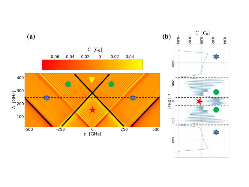
Figure 2: (a) Parametric capacitance $C$ of the DQD as a function of the excitation field amplitude $A$ and the energy detuning $\varepsilon$. This value is calculated in units of $C_{0}$. (b) Dependence of the parametric capacitance of the DQD on the energy detuning $\varepsilon$ for the excitation field amplitude $A\leavevmode\nobreak\ =\leavevmode\nobreak\ 240\,\mathrm{GHz}$ (a line cut of panel (a) along $y$-axis). The corresponding relaxation rates of the system are $\Gamma_{1}\leavevmode\nobreak\ =\leavevmode\nobreak\ 0.9\,\mathrm{GHz}$, $\Gamma_{\rm R}\leavevmode\nobreak\ =\leavevmode\nobreak\ 12\,\mathrm{GHz}$, $\Gamma_{\rm L}\leavevmode\nobreak\ =\leavevmode\nobreak\ 50\,\mathrm{MHz}$. The energy splittings are equal to $\mathrm{\Delta}_{\rm c}\leavevmode\nobreak\ =\leavevmode\nobreak\ 8.25\,\mathrm{GHz}$, $\mathrm{\Delta}^{\rm down}\leavevmode\nobreak\ =\leavevmode\nobreak\ 21\,\mathrm{GHz}$, $\mathrm{\Delta}^{\rm up}\leavevmode\nobreak\ =\leavevmode\nobreak\ 1\,\mathrm{GHz}$, and their positions are at $\varepsilon_{\mathrm{c}}\leavevmode\nobreak\ =\leavevmode\nobreak\ 0\,\mathrm{}$, $\varepsilon_{00}^{\rm down}=\leavevmode\nobreak\ -276\,\mathrm{GHz}$, $\varepsilon_{11}^{\rm down}=\leavevmode\nobreak\ 276\,\mathrm{GHz}$, $\varepsilon_{00}^{\rm up}=\leavevmode\nobreak\ -255\,\mathrm{GHz}$, $\varepsilon_{11}^{\rm up}=\leavevmode\nobreak\ 255\,\mathrm{GHz}$. The decoherence rate $\Gamma_{2}\leavevmode\nobreak\ =\leavevmode\nobreak\ 4\,\mathrm{GHz}$ and the excitation frequency $\nu\leavevmode\nobreak\ =\leavevmode\nobreak\ 4\,\mathrm{GHz}$.

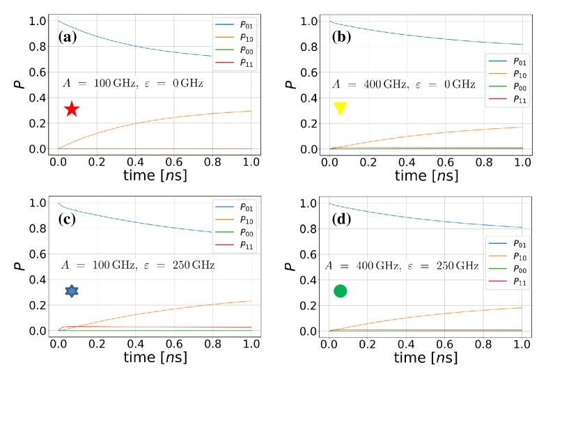
Figure 3: Time dependence of probabilities for different regimes: (a) multi-passage LZSM; (b) single-passage LZSM; (c) incoherent LZSM; (d) double-passage LZSM. The parameters are the same with Fig. 2.

By solving Eqs. (6, 7) for the stationary regime (when $dP_{ij}/dt=0$), we obtain $P_{mn}=P_{mn}(\varepsilon,A)$, $m,n=0,1$, as a function of $\varepsilon$ and $A$ what allows us to analyze the experimentally measured value, the phase response of the resonator $\mathrm{\Delta}\phi$, which according to Ref. [Chatterjee et al., 2018] can be written as

$$\mathrm{\Delta}\phi=-\pi Q\frac{C}{C_{\rm p}},$$ (8)

where $C_{\rm p}\leavevmode\nobreak\ =\leavevmode\nobreak\ 660\,\mathrm{fF}$ is the parasitic capacitance to ground of the device, $Q=42$ is the loaded Q-factor of the resonator, $C$ is the parametric capacitance of a DQD which can be calculated by the following expression

$$C\leavevmode\nobreak\ =\leavevmode\nobreak\ C_{0}\frac{d}{d\varepsilon}\left\{P_{01}-P_{10}+\alpha\left(P_{00}-P_{11}\right)\right\},$$ (9)

where $\alpha$ is a dimensionless factor which describes the DQD coupling to the fermionic sea, for the experiment of Ref. [Chatterjee et al., 2018] $\alpha\leavevmode\nobreak\ =\leavevmode\nobreak\ 18$ and $C_{0}$ is the constant proportionality factor. In our calculations we plot the parametric capacitance $C$ as a function of $\varepsilon$, and $A$. The results of the theoretical calculations are presented in Fig. 2(a). The obtained interferogram shows the patterns similar to the experimental ones (see Fig. 3(b) in Ref. [Chatterjee et al., 2018]). Specifically, one can see four different regimes: incoherent one (blue star), double-passage LZSM (green circle), single-passage LZSM (yellow triangle), multi-passage LZSM (red star). Fig. 2(b) presents a line cut of Fig. 2(a) at $A\leavevmode\nobreak\ =\leavevmode\nobreak\ 240\,\mathrm{GHz}$, the same patterns can be seen in the experiment (see Fig. 3(c) in Ref. [Chatterjee et al., 2018]).

Figure 3 shows time dependence of probabilities for different regimes: (a) multi-passage LZSM; (b) single-passage LZSM; (c) incoherent one; (d) double-passage LZSM. From the plots, one can conclude that the stationary regime (when $dP_{ij}/dt\leavevmode\nobreak\ \approx\leavevmode\nobreak\ 0$) starts after $t_{0}\leavevmode\nobreak\ \approx\leavevmode\nobreak\ 0.8\,\mathrm{ns}$. Also, it could be seen that for all cases $P_{01}>P_{10}\gg P_{11},P_{00}$.

IV Three-level approximation of the DQD

In this section, we consider the system in the energy basis (in the previous section, the system was described in the charge basis) with the basis states $E_{0},\leavevmode\nobreak\ E_{1},\leavevmode\nobreak\ E_{2},\leavevmode\nobreak\ E_{3}$ and probabilities to occupy the corresponding energy state $P_{0},\leavevmode\nobreak\ P_{1},\leavevmode\nobreak\ P_{2},\leavevmode\nobreak\ P_{3}$. The corresponding energy-level diagram is shown in Fig. 4. In the considered case, we can neglect the highest energy level ($P_{3}=0$) and take into account only three levels. Our energy-level diagram has five avoided level crossings at $\varepsilon_{\mathrm{c}}\leavevmode\nobreak\ =\leavevmode\nobreak\ 0\,\mathrm{}$, $\varepsilon_{00}^{\rm down}=\leavevmode\nobreak\ -276\,\mathrm{GHz}$, $\varepsilon_{11}^{\rm down}=\leavevmode\nobreak\ 276\,\mathrm{GHz}$, $\varepsilon_{00}^{\rm up}=\leavevmode\nobreak\ -255\,\mathrm{GHz}$, $\varepsilon_{11}^{\rm up}=\leavevmode\nobreak\ 255\,\mathrm{GHz}$.

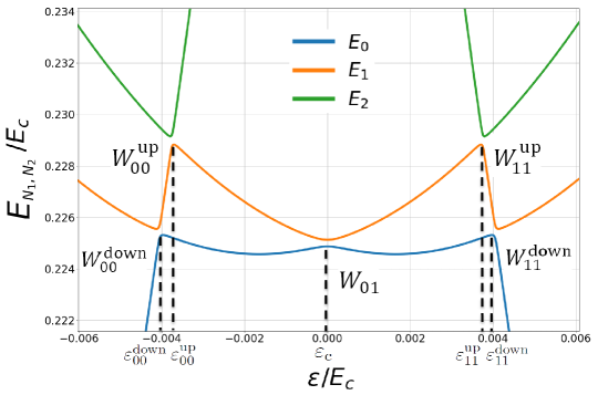
Figure 4: Energy levels of the DQD in the energy basis. This plot is a representation of Fig. 1(b) in the energy basis. The value $W_{01}$ indicates transition rate between energy states $E_{1}$ and $E_{0}$ at $\varepsilon\leavevmode\nobreak\ =\leavevmode\nobreak\ \varepsilon_{\rm c}$, $W_{00}^{\rm down}$ and $W_{11}^{\rm down}$ indicate transition rates between energy states $E_{1}$ and $E_{0}$ at $\varepsilon\leavevmode\nobreak\ =\leavevmode\nobreak\ \varepsilon_{00}^{\rm down}$ and $\varepsilon_{11}^{\rm down}$, respectively, $W_{00}^{\rm up}$ and $W_{11}^{\rm up}$ indicate transition rates between energy states $E_{1}$ and $E_{2}$ at $\varepsilon\leavevmode\nobreak\ =\leavevmode\nobreak\ \varepsilon_{00}^{\rm up}$ and $\varepsilon_{11}^{\rm up}$, respectively.

The rate equations (5) take the form

$$\left\{\begin{array}[]{c}\frac{dP_{0}}{dt}=\left[W_{\mathrm{01}}+W_{00}^{\rm down}+W_{11}^{\rm down}\right]\left(P_{1}-P_{0}\right)+\Gamma_{1\rightarrow 0}P_{1},\\ \frac{dP_{1}}{dt}=\left[W_{\mathrm{01}}+W_{00}^{\rm down}+W_{11}^{\rm down}\right]\left(P_{0}-P_{1}\right)+\\ +\left[W_{00}^{\rm up}+W_{11}^{\rm up}\right]\left(P_{2}-P_{1}\right)-\Gamma_{1\rightarrow 0}P_{1},\\ P_{0}+P_{1}+P_{2}=1.\end{array}\right.$$ (10)

These equations contain only leading terms; in particular, we omitted the term $\Gamma_{2\rightarrow 0}P_{2}$ in the first equation and the term $\Gamma_{2\rightarrow 1}P_{2}$ in the second equation. The fact that there are different relaxations between different levels is taken into account by assuming the time-dependent relaxation $\Gamma_{1\rightarrow 0}=\Gamma_{1\rightarrow 0}(t)$:

$$\Gamma_{1\rightarrow 0}(t)=\left\{\begin{array}[]{c}\Gamma_{1},\text{ \ }\left|\varepsilon(t)\right|<\varepsilon_{00}^{\rm down},\\ \Gamma_{\mathrm{L}},\text{ }\ \left|\varepsilon(t)\right|>\varepsilon_{00}^{\rm down},\end{array}\right.$$ (11)

where the first line describes the inter-dot relaxation, while the second line corresponds to the tunneling between the left dot and the leads.

Relation (11) provides two simplifications, when the whole dynamics is either for $\left|\varepsilon(t)\right|<\varepsilon_{00}^{\rm up}$ or for $\ \left|\varepsilon(t)\right|>\varepsilon_{00}^{\rm up}$. In these cases $\Gamma_{1\rightarrow 0}$ becomes independent of time and we can have the stationary solution of the system of equations (10). (Then we can have the recipe for alike situations: take the analytical solutions for such regions, then fitting with this is a simple way to get the parameters; and afterward, one can continue with more elaborated calculations, such as solving time-dependent equations.) In these two particular cases we obtain analytical stationary solutions. For the coherent regime (“red-star” region) we have $W_{00}^{\rm down}$, $W_{00}^{\rm up}$, $W_{11}^{\rm down}$ and $W_{11}^{\rm up}$ $\rightarrow 0$ and $P_{2}\rightarrow 0$, and then, it follows [Berns et al., 2006; Ivakhnenko et al., 2023]

$$P_{1} = \frac{1}{2}\sum_{n=-\infty}^{\infty}\frac{\mathrm{\Delta}_{\mathrm{c},n}^{2}}{\mathrm{\Delta}_{\mathrm{c},n}^{2}+\frac{\Gamma_{1}}{\Gamma_{2}}\left((\varepsilon-\varepsilon_{\mathrm{c}})-n\nu\right)^{2}+\Gamma_{1}\Gamma_{2}},$$ (12)

$$\mathrm{\Delta}_{\mathrm{c},n} = \mathrm{\Delta}_{\mathrm{c}}J_{n}\left(\frac{A}{\nu}\right).$$

Analogously, for the incoherent regime (“blue-star” region) nearby the point $\varepsilon=\varepsilon_{00}^{\mathrm{down}}$ we have $W_{01},W_{00}^{\rm up},W_{11}^{\rm up}$ and $W_{11}^{\rm down}\rightarrow 0$ and $P_{2}\rightarrow 0$, therefore, then it follows

$$P_{1} = \frac{1}{2}\sum_{n=-\infty}^{\infty}\frac{(\mathrm{\Delta}_{n}^{\rm down})^{2}}{(\mathrm{\Delta}_{n}^{\rm down})^{2}+\frac{\Gamma_{\mathrm{L}}}{\Gamma_{2,L}}\left((\varepsilon-\varepsilon_{00}^{\mathrm{down}})-n\nu\right)^{2}+\Gamma_{\mathrm{L}}\Gamma_{2,L}},$$ (13)

$$\mathrm{\Delta}_{n}^{\rm down} = \mathrm{\Delta}^{\rm down}J_{n}\left(\frac{A}{\nu}\right).$$

We can also note that in the lower parts of the $(\varepsilon,A)$ plane, below the red-star and the blue-star regions, all $W$’s are $0$, and we have $P_{i}$ being all constants, resulting in zero $C$.

V Conclusions

We considered the rate-equation approach for a theoretical description of the four-level DQD. The system state as a function of the energy detuning $\varepsilon$ and the amplitude of the excitation signal $A$ was studied. We obtained that the DQD can be operated in four regimes in dependence on the considered parameters. These regimes are single-passage LZSM, which corresponds to small $\varepsilon$ and large $A$; double-passage LZSM (large $A$ and medium $\varepsilon$); multi-passage LZSM (small $A$ and $\varepsilon$); incoherent regime (large $\varepsilon$ and small $A$). Our research gives information about the DQD properties and behavior which could be used for the system initializing and controlling.

Appendix A Energy levels of a parallel double-quantum dot

In the current research we study the DQD proposed in Ref. [Chatterjee et al., 2018], see Fig. 1(a). The first step in the system analysis is finding of the DQD energy levels. In the general form system electrostatic energy can be written by

$$E=\frac{1}{2}\overrightarrow{V}\cdot\mathbf{C}\overrightarrow{V}=\frac{1}{2}\overrightarrow{V}\cdot\overrightarrow{Q}=\frac{1}{2}\overrightarrow{Q}\cdot\mathbf{C}^{-1}\overrightarrow{Q},$$ (14)

where $\overrightarrow{V}$ and $\overrightarrow{Q}$ are the vectors of voltages and charges, respectively, $\mathbf{C}$ is the capacitance matrix. In Eq. (14) we used $\overrightarrow{Q}=\mathbf{C}\overrightarrow{V}$. Thus, to obtain the system energy levels, we need to find the vector of charges and the inverse capacitance matrix of the system.

The charges $Q_{1,2}$ in the quantum dots can be written as follows

$$Q_{1} = C_{\rm T1}(V_{1}-V_{\rm TG})+C_{\rm B1}(V_{1}-V_{\rm BG})+C_{\rm S}(V_{1}-V_{\rm S})+$$ (15)

$$+C_{\rm D}(V_{1}-V_{\rm D})+C_{\rm M}(V_{1}-V_{2}),$$

$$Q_{2} = C_{\rm T2}(V_{2}-V_{\rm TG})+C_{\rm B2}(V_{2}-V_{\rm BG})+C_{\rm S}(V_{2}-V_{\rm S})+$$ (16)

$$+C_{\rm D}(V_{2}-V_{\rm D})+C_{\rm M}(V_{2}-V_{1}).$$

It is convenient to rewrite expressions (15, 16) in a matrix form

$$\overrightarrow{Q} = \begin{pmatrix}Q_{1}+C_{\rm T1}V_{\rm TG}+C_{\rm B1}V_{\rm BG}+C_{\rm S}V_{\rm S}+C_{\rm D}V_{\rm D}\\ Q_{2}+C_{\rm T2}V_{\rm TG}+C_{\rm B2}V_{\rm BG}+C_{\rm S}V_{\rm S}+C_{\rm D}V_{\rm D}\end{pmatrix}=$$ (17)

$$\begin{pmatrix}C_{1}V_{1}-C_{\rm M}V_{2}\\ C_{2}V_{2}-C_{\rm M}V_{1}\end{pmatrix},$$

where $C_{1}$ and $C_{2}$ are the capacitances, connected to the first and the second quantum dots, respectively,

$$C_{1} = C_{\rm T1}+C_{\rm B1}+C_{\rm D}+C_{\rm S}+C_{\rm M},$$ (18)

$$C_{2} = C_{\rm T2}+C_{\rm B2}+C_{\rm D}+C_{\rm S}+C_{\rm M}.$$

Then the capacitance matrix has the following form:

$$\mathbf{C}=\begin{pmatrix}C_{1}&-C_{\rm M}\\ -C_{\rm M}&C_{2}\end{pmatrix}.$$ (19)

Let us assume for simplicity that $V_{\rm S}=V_{\rm D}=0$. Then putting expressions for the vector of charges Eq. (17) and for the inverse capacitance matrix Eq. (19), for the DQD electrostatic energy we obtain:

$$E = \frac{1}{C_{1}C_{2}-C_{\rm M}^{2}}\left[\frac{1}{2}C_{1}Q_{2}^{2}+\frac{1}{2}C_{2}Q_{1}^{2}+C_{\rm M}Q_{1}Q_{2}\right]+\frac{V_{\rm TG}}{C_{1}C_{2}-C_{\rm M}^{2}}\left[C_{\rm T1}\left(C_{\rm M}Q_{2}+C_{2}Q_{1}\right)+C_{\rm T2}\left(C_{1}Q_{2}+C_{\rm M}Q_{1}\right)\right]+$$ (20)

$$\frac{V_{\rm BG}}{C_{1}C_{2}-C_{\rm M}^{2}}\left[C_{\rm B1}\left(C_{\rm M}Q_{2}+C_{2}Q_{1}\right)+C_{\rm B2}\left(C_{1}Q_{2}+C_{\rm M}Q_{1}\right)\right]+\frac{V_{\rm TG}^{2}}{C_{1}C_{2}-C_{\rm M}^{2}}\left[\frac{1}{2}C_{1}C_{\rm T2}^{2}+\frac{1}{2}C_{2}C_{\rm T1}^{2}+C_{\rm T1}C_{\rm T2}C_{\rm M}\right]+$$

$$\frac{V_{\rm BG}^{2}}{C_{1}C_{2}-C_{\rm M}^{2}}\left[\frac{1}{2}C_{1}C_{\rm T2}^{2}+\frac{1}{2}C_{2}C_{\rm T1}^{2}+C_{\rm T1}C_{\rm T2}C_{\rm M}\right].$$

To simplify Eq. (20), let us introduce new values, $N_{i}=-\frac{Q_{i}}{\left|e\right|}$, for the number of electrons in the $i$th quantum dot, and reduced top-gate $n_{t}$ and back-gate $n_{b}$ voltages

$$n_{t} = \frac{C_{\rm T1}V_{\rm TG}}{\left|e\right|}=\frac{1}{1+a}\frac{C_{\rm T2}V_{\rm TG}}{\left|e\right|},$$ (21)

$$n_{b} = \frac{C_{\rm B1}V_{\rm BG}}{\left|e\right|}=\frac{1}{1-a}\frac{C_{\rm B2}V_{\rm BG}}{\left|e\right|},$$ (22)

where $a$ is an asymmetry factor in the gate couplings. Assuming $C_{1}=C_{2}=mC_{\rm M}$ and rewriting the quantum dot charges as $Q_{1(2)}=-\left|e\right|N_{1(2)}$, then for the energy of the quantum dot, we have

$$\frac{E_{N_{1},N_{2}}}{E_{\rm C}} = \frac{1}{2}N_{1}^{2}+\frac{1}{2}N_{2}^{2}+\frac{N_{1}N_{2}}{m}-n_{t}\left[N_{1}+\frac{N_{2}}{m}+(1+a)\left(N_{2}+\frac{N_{1}}{m}\right)\right]$$ (23)

$$-n_{b}\left[N_{1}+\frac{N_{2}}{m}+(1-a)\left(N_{2}+\frac{N_{1}}{m}\right)\right]+n_{t}^{2}\left[\frac{1}{2}+\frac{1}{2}(1+a)^{2}+\frac{1+a}{m}\right]$$

$$+n_{b}^{2}\left[\frac{1}{2}+\frac{1}{2}(1-a)^{2}+\frac{1-a}{m}\right]+n_{t}n_{b}\left[2(1+\frac{1}{m})-a^{2}\right],$$

where we defined $E_{\rm C}=E_{\rm C_{1}}=E_{\rm C_{2}}=mE_{\rm C_{M}}=e^{2}\frac{C_{1}}{{C_{1}^{2}-C_{\rm M}^{2}}}$. We plot the energy-level diagram in Fig. 1(b) for the following parameters: $a=0.1$, $n_{b}=0.25$, $m=10$, and $N_{1},\leavevmode\nobreak\ N_{2}$ are equal to $0$ or $1$.

Data availability

All data generated or analyzed during this study are included in this published article.

References

- Veldhorst et al. (2014) M. Veldhorst, J. C. C. Hwang, C. H. Yang, A. W. Leenstra, B. de Ronde, J. P. Dehollain, J. T. Muhonen, F. E. Hudson, K. M. Itoh, A. Morello, and A. S. Dzurak, “An addressable quantum dot qubit with fault-tolerant control-fidelity,” Nat. Nanotechnol. 9, 981–985 (2014).
- Shulman et al. (2012) M. D. Shulman, O. E. Dial, S. P. Harvey, H. Bluhm, V. Umansky, and A. Yacoby, “Demonstration of entanglement of electrostatically coupled singlet-triplet qubits,” Science 336, 202–205 (2012).
- Petta et al. (2005) J. R. Petta, A. C. Johnson, J. M. Taylor, E. A. Laird, A. Yacoby, M. D. Lukin, C. M. Marcus, M. P. Hanson, and A. C. Gossard, “Coherent manipulation of coupled electron spins in semiconductor quantum dots,” Science 309, 2180–2184 (2005).
- Hanson et al. (2005) R. Hanson, L. H. W. van Beveren, I. T. Vink, J. M. Elzerman, W. J. M. Naber, F. H. L. Koppens, L. P. Kouwenhoven, and L. M. K. Vandersypen, “Single-shot readout of electron spin states in a quantum dot using spin-dependent tunnel rates,” Phys. Rev. Lett. 94, 196802 (2005).
- Kiyama et al. (2016) H. Kiyama, T. Nakajima, S. Teraoka, A. Oiwa, and S. Tarucha, “Single-shot ternary readout of two-electron spin states in a quantum dot using spin filtering by quantum hall edge states,” Phys. Rev. Lett. 117, 236802 (2016).
- Friesen et al. (2004) M. Friesen, C. Tahan, R. Joynt, and M. A. Eriksson, “Spin readout and initialization in a semiconductor quantum dot,” Phys. Rev. Lett. 92, 037901 (2004).
- Cerletti et al. (2005) V. Cerletti, W. A. Coish, O. Gywat, and D. Loss, “Recipes for spin-based quantum computing,” Nanotechnology 16, R27 (2005).
- Loss and DiVincenzo (1998) D. Loss and D. P. DiVincenzo, “Quantum computation with quantum dots,” Phys. Rev. A 57, 120–126 (1998).
- DiVincenzo et al. (2000) D. P. DiVincenzo, D. Bacon, J. Kempe, G. Burkard, and K. B. Whaley, “Universal quantum computation with the exchange interaction,” Nature 408, 339–342 (2000).
- Byrd and Lidar (2002) M. S. Byrd and D. A. Lidar, “Comprehensive encoding and decoupling solution to problems of decoherence and design in solid-state quantum computing,” Phys. Rev. Lett. 89, 047901 (2002).
- Kim (1998) K. Kim, “Visible light emissions and single-electron tunneling from silicon quantum dots embedded in Si-rich deposited in plasma phase,” Phys. Rev. B 57, 13072–13076 (1998).
- Romero and van de Lagemaat (2009) M. J. Romero and J. van de Lagemaat, “Luminescence of quantum dots by coupling with nonradiative surface plasmon modes in a scanning tunneling microscope,” Phys. Rev. B 80, 115432 (2009).
- Estrada Saldaña et al. (2018) J. C. Estrada Saldaña, A. Vekris, G. Steffensen, R. Žitko, P. Krogstrup, J. Paaske, K. Grove-Rasmussen, and J. Nygård, “Supercurrent in a double quantum dot,” Phys. Rev. Lett. 121, 257701 (2018).
- Sasaki et al. (2004) S. Sasaki, S. Amaha, N. Asakawa, M. Eto, and S. Tarucha, “Enhanced Kondo effect via tuned orbital degeneracy in a spin artificial atom,” Phys. Rev. Lett. 93, 017205 (2004).
- Beenakker and Staring (1992) C. W. J. Beenakker and A. A. M. Staring, “Theory of the thermopower of a quantum dot,” Phys. Rev. B 46, 9667–9676 (1992).
- Simon et al. (2007) C. Simon, Y.-M. Niquet, X. Caillet, J. Eymery, J.-P. Poizat, and J.-M. Gérard, “Quantum communication with quantum dot spins,” Phys. Rev. B 75, 081302 (2007).
- Huwer et al. (2017) J. Huwer, R. M. Stevenson, J. Skiba-Szymanska, M. B. Ward, A. J. Shields, M. Felle, I. Farrer, D. A. Ritchie, and R. V. Penty, “Quantum-dot-based telecommunication-wavelength quantum relay,” Phys. Rev. Appl. 8, 024007 (2017).
- Abolfath et al. (2008) R. M. Abolfath, A. G. Petukhov, and I. Žutić, “Piezomagnetic quantum dots,” Phys. Rev. Lett. 101, 207202 (2008).
- Flentje et al. (2017) H. Flentje, P.-A. Mortemousque, R. Thalineau, A. Ludwig, A. D. Wieck, C. Bauerle, and T. Meunier, “Coherent long-distance displacement of individual electron spins,” Nat. Commun. 8 (2017).
- Brandes (2005) T. Brandes, “Coherent and collective quantum optical effects in mesoscopic systems,” Phys. Rep. 408, 315–474 (2005).
- van der Wiel et al. (2002) W. G. van der Wiel, S. De Franceschi, J. M. Elzerman, T. Fujisawa, S. Tarucha, and L. P. Kouwenhoven, “Electron transport through double quantum dots,” Rev. Mod. Phys. 75, 1–22 (2002).
- Awschalom and Flatte (2007) D. Awschalom and M. Flatte, “Challenges for semiconductor spintronics,” Nature Phys. 3, 153 (2007).
- Donsa et al. (2014) S. Donsa, S. Andergassen, and K. Held, “Double quantum dot as a minimal thermoelectric generator,” Phys. Rev. B 89, 125103 (2014).
- Aguado and Kouwenhoven (2000) R. Aguado and L. P. Kouwenhoven, “Double quantum dots as detectors of high-frequency quantum noise in mesoscopic conductors,” Phys. Rev. Lett. 84, 1986–1989 (2000).
- Liu et al. (2017) T. Liu, Q.-P. Su, J.-H. Yang, Y. Zhang, S.-J. Xiong, J.-M. Liu, and C.-P. Yang, “Transferring arbitrary d-dimensional quantum states of a superconducting transmon qudit in circuit QED,” Sci. Rep. 7 (2017).
- Wang et al. (2020) Y. Wang, Z. Hu, B. C. Sanders, and S. Kais, “Qudits and high-dimensional quantum computing,” Front. Phys. 8 (2020).
- Han et al. (2019) Y. Han, X.-Q. Luo, T.-F. Li, W. Zhang, S.-P. Wang, J. Tsai, F. Nori, and J. You, “Time-domain grating with a periodically driven qutrit,” Phys. Rev. Appl. 11, 014053 (2019).
- Kononenko et al. (2021) M. Kononenko, M. A. Yurtalan, S. Ren, J. Shi, S. Ashhab, and A. Lupascu, “Characterization of control in a superconducting qutrit using randomized benchmarking,” Phys. Rev. Res. 3, L042007 (2021).
- Yurtalan et al. (2020) M. A. Yurtalan, J. Shi, M. Kononenko, A. Lupascu, and S. Ashhab, “Implementation of a Walsh-Hadamard gate in a superconducting qutrit,” Phys. Rev. Lett. 125, 180504 (2020).
- Chatterjee et al. (2018) A. Chatterjee, S. N. Shevchenko, S. Barraud, R. M. Otxoa, F. Nori, J. J. L. Morton, and M. F. Gonzalez-Zalba, “A silicon-based single-electron interferometer coupled to a fermionic sea,” Phys. Rev. B 97, 045405 (2018).
- Ferrón et al. (2012) A. Ferrón, D. Domínguez, and M. J. Sánchez, “Tailoring population inversion in Landau-Zener-Stückelberg interferometry of flux qubits,” Phys. Rev. Lett. 109, 237005 (2012).
- Ferrón et al. (2016) A. Ferrón, D. Domínguez, and M. J. Sánchez, “Dynamic transition in Landau-Zener-Stückelberg interferometry of dissipative systems: The case of the flux qubit,” Phys. Rev. B 93, 064521 (2016).
- Liul and Shevchenko (2023) M. P. Liul and S. N. Shevchenko, “Rate-equation approach for multi-level quantum systems,” Low Temp. Phys. 49, 102–108 (2023).
- Berns et al. (2006) D. M. Berns, W. D. Oliver, S. O. Valenzuela, A. V. Shytov, K. K. Berggren, L. S. Levitov, and T. P. Orlando, “Coherent quasiclassical dynamics of a persistent current qubit,” Phys. Rev. Lett. 97, 150502 (2006).
- Oliver and Valenzuela (2009) W. D. Oliver and S. O. Valenzuela, “Large-amplitude driving of a superconducting artificial atom,” Quantum Inf. Process. 8, 261–281 (2009).
- Wen and Yu (2009) X. Wen and Y. Yu, “Landau-Zener interference in multilevel superconducting flux qubits driven by large-amplitude fields,” Phys. Rev. B 79 (2009).
- Izmalkov et al. (2004) A. Izmalkov, M. Grajcar, E. Il’ichev, N. Oukhanski, T. Wagner, H.-G. Meyer, W. Krech, M. H. S. Amin, A. M. van den Brink, and A. M. Zagoskin, “Observation of macroscopic Landau-Zener transitions in a superconducting device,” Europhys. Lett. 65, 844–849 (2004).
- Ashhab (2014) S. Ashhab, “Landau-Zener transitions in a two-level system coupled to a finite-temperature harmonic oscillator,” Phys. Rev. A 90, 062120 (2014).
- Nakonechnyi et al. (2021) M. A. Nakonechnyi, D. S. Karpov, A. N. Omelyanchouk, and S. N. Shevchenko, “Multi-signal spectroscopy of qubit-resonator systems,” Low Temp. Phys. 37, 383 (2021).
- Liul et al. (2023) M. P. Liul, C.-H. Chien, C.-Y. Chen, P. Y. Wen, J. C. Chen, Y.-H. Lin, S. N. Shevchenko, F. Nori, and I.-C. Hoi, “Coherent dynamics of a photon-dressed qubit,” Phys. Rev. B 107, 195441 (2023).
- Fuchs et al. (2011) G. Fuchs, G. Burkard, P. Klimov, and D. Awschalom, “A quantum memory intrinsic to single nitrogen-vacancy centres in diamond,” Nature Phys. 7, 789–793 (2011).
- Ribeiro and Burkard (2009) H. Ribeiro and G. Burkard, “Nuclear state preparation via Landau-Zener-Stückelberg transitions in double quantum dots,” Phys. Rev. Lett. 102, 216802 (2009).
- Thiel (1990) A. Thiel, “The Landau-Zener effect in nuclear molecules,” J. Phys. G: Nucl. Part. Phys. 16, 867–910 (1990).
- Zhu et al. (1997) L. Zhu, A. Widom, and P. M. Champion, “A multidimensional Landau-Zener description of chemical reaction dynamics and vibrational coherence,” J. Chem. Phys. 107, 2859–2871 (1997).
- Bouwmeester et al. (1995) D. Bouwmeester, N. H. Dekker, F. E. v. Dorsselaer, C. A. Schrama, P. M. Visser, and J. P. Woerdman, “Observation of Landau-Zener dynamics in classical optical systems,” Phys. Rev. A 51, 646–654 (1995).
- Stehlik et al. (2012) J. Stehlik, Y. Dovzhenko, J. R. Petta, J. R. Johansson, F. Nori, H. Lu, and A. C. Gossard, “Landau-Zener-Stückelberg interferometry of a single electron charge qubit,” Phys. Rev. B 86, 121303 (2012).
- Oliver et al. (2005) W. D. Oliver, Y. Yu, J. C. Lee, K. K. Berggren, L. S. Levitov, and T. P. Orlando, “Mach-Zehnder interferometry in a strongly driven superconducting qubit,” Science 310, 1653–1657 (2005).
- Gonzalez-Zalba et al. (2016) M. F. Gonzalez-Zalba, S. N. Shevchenko, S. Barraud, J. R. Johansson, A. J. Ferguson, F. Nori, and A. C. Betz, “Gate-sensing coherent charge oscillations in a silicon field-effect transistor,” Nano Lett. 16, 1614–1619 (2016).
- Kofman et al. (2023) P. O. Kofman, O. V. Ivakhnenko, S. N. Shevchenko, and F. Nori, “Majorana’s approach to nonadiabatic transitions validates the adiabatic-impulse approximation,” Sci. Rep. 13, 5053 (2023).
- Ono et al. (2019) K. Ono, S. N. Shevchenko, T. Mori, S. Moriyama, and F. Nori, “Quantum interferometry with a -factor-tunable spin qubit,” Phys. Rev. Lett. 122, 207703 (2019).
- Wu et al. (2019) T. Wu, Y. Zhou, Y. Xu, S. Liu, and J. Li, “Landau-Zener-Stückelberg interference in nonlinear regime,” Chin. Phys. Lett. 36, 124204 (2019).
- Ivakhnenko et al. (2023) O. V. Ivakhnenko, S. N. Shevchenko, and F. Nori, “Nonadiabatic Landau-Zener-Stückelberg-Majorana transitions, dynamics and interference,” Phys. Rep. 995, 1–89 (2023).
- Nakamura and Tsai (1999) Y. Nakamura and J. S. Tsai, “A coherent two-level system in a superconducting single-electron transistor observed through photon-assisted Cooper-pair tunneling,” J. Supercond. 12, 799–806 (1999).
- Rudner et al. (2008) M. S. Rudner, A. V. Shytov, L. S. Levitov, D. M. Berns, W. D. Oliver, S. O. Valenzuela, and T. P. Orlando, “Quantum phase tomography of a strongly driven qubit,” Phys. Rev. Lett. 101, 190502 (2008).
- Malla and Raikh (2022) R. K. Malla and M. Raikh, “Landau-Zener transition between two levels coupled to continuum,” Phys. Lett. A 445, 128249 (2022).
- Chen et al. (2011) J.-D. Chen, X.-D. Wen, G.-Z. Sun, and Y. Yu, “Landau-Zener-Stückelberg interference in a multi-anticrossing system,” Chin. Phys. B 20, 088501 (2011).
- Wang et al. (2010) Y. Wang, S. Cong, X. Wen, C. Pan, G. Sun, J. Chen, L. Kang, W. Xu, Y. Yu, and P. Wu, “Quantum interference induced by multiple Landau-Zener transitions in a strongly driven rf-squid qubit,” Phys. Rev. B 81, 144505 (2010).
- Wen et al. (2010) X. Wen, Y. Wang, S. Cong, G. Sun, J. Chen, L. Kang, W. Xu, Y. Yu, P. Wu, and S. Han, “Landau-Zener-Stuckelberg interferometry in multilevel superconducting flux qubit,” arXiv (2010).
- Otxoa et al. (2019) R. M. Otxoa, A. Chatterjee, S. N. Shevchenko, S. Barraud, F. Nori, and M. F. Gonzalez-Zalba, “Quantum interference capacitor based on double-passage Landau-Zener-Stückelberg-Majorana interferometry,” Phys. Rev. B 100, 205425 (2019).
- He et al. (2023) J. He, D. Pan, M. Liu, Z. Lyu, Z. Jia, G. Yang, S. Zhu, G. Liu, J. Shen, S. N. Shevchenko, F. Nori, J. Zhao, L. Lu, and F. Qu, “Quantifying quantum coherence of multiple-charge states in tunable Josephson junctions,” arXiv (2023).