Nearest-Neighbor Sampling Based Conditional Independence Testing

Abstract

The conditional randomization test (CRT) was recently proposed to test whether two random variables $X$ and $Y$ are conditionally independent given random variables $Z$. The CRT assumes that the conditional distribution of $X$ given $Z$ is known under the null hypothesis and then it is compared to the distribution of the observed samples of the original data. The aim of this paper is to develop a novel alternative of CRT by using nearest-neighbor sampling without assuming the exact form of the distribution of $X$ given $Z$. Specifically, we utilize the computationally efficient 1-nearest-neighbor to approximate the conditional distribution that encodes the null hypothesis. Then, theoretically, we show that the distribution of the generated samples is very close to the true conditional distribution in terms of total variation distance. Furthermore, we take the classifier-based conditional mutual information estimator as our test statistic. The test statistic as an empirical fundamental information theoretic quantity is able to well capture the conditional-dependence feature. We show that our proposed test is computationally very fast, while controlling type I and II errors quite well. Finally, we demonstrate the efficiency of our proposed test in both synthetic and real data analyses.

Introduction

Conditional independence testing (CIT) has wide applications in statistics and machine learning, including causal inference (Spirtes et al. 2000; Pearl 2009; Cai, Li, and Zhang 2022) and graphical models (Lauritzen 1996; Koller and Friedman 2009) as two well-known examples. The aim of this paper is to develop a flexible and fast method for CIT. Specifically, we consider two univariate continuous random variables $X$ and $Y$, and a set of random variables $Z\in R^{d_{Z}}$, whose dimension $d_{Z}$ can potentially diverge to infinity, with a joint density function given by $p_{X,Y,Z}(x,y,z)$. Based on $n$ independently and identically distributed (i.i.d) copies $\{(X_{i},Y_{i},Z_{i}):i=1,\ldots,n\}$ of $(X,Y,Z)$, we are interested in testing whether two random variables $X$ and $Y$ are conditionally independent given $Z$; that is,

$$H_{0}:X\perp\!\!\!\perp Y|Z~{}~{}\mbox{versus}~{}~{}H_{1}:X\not\!\perp\!\!\!\perp Y|Z,$$

where $\perp\!\!\!\perp$ denotes the independence. The high dimensionality of $Z$ makes CIT challenging (Bellot and van der Schaar 2019; Shi et al. 2021). Our proposed method can be readily extended to the scenario of multivariate $X$ and $Y$.

Recently, many methods have been proposed to test conditional independence. See, for example, Candes et al. (2018), Zhang et al. (2011), Zhang et al. (2017), Bellot and van der Schaar (2019), Strobl, Zhang, and Visweswaran (2019), Berrett et al. (2020), Shah and Peters (2020), Shi et al. (2021), and Zhang et al. (2022). Among them, the conditional randomization test (CRT) proposed by Candes et al. (2018) is one of the most important methods, but CRT assumes that the true conditional distribution $p_{X|Z}$ is known. Conditional on $\{Z_{1},\ldots,Z_{n}\}$, one can independently draw $X_{i}^{(m)}\sim p_{X|Z=Z_{i}}$ for each $i$ across $m=1,\ldots,M$ such that all $\bm{X}^{(m)}:=(X_{1}^{(m)},\ldots,X_{n}^{(m)})$ are independent of $\bm{X}:=(X_{1},\ldots,X_{n})$ and $\bm{Y}:=(Y_{1},\ldots,Y_{n})$, where $M$ is the number of repetitions. Thus, under the null hypothesis $H_{0}:X\perp\!\!\!\perp Y|Z$, we have $(X^{(m)},Y,Z)\overset{d}{=}(X,Y,Z)$ for all $m$, where $\overset{d}{=}$ denotes equality in distribution. A large difference between $(X^{(m)},Y,Z)$ and $(X,Y,Z)$ can be regarded as a strong evidence against $H_{0}$. Statistically, one can consider a test statistic $T(\bm{X},\bm{Y},\bm{Z})$ and approximate its $p$-value by

$$\frac{1+\sum_{m=1}^{M}{I}(T(\bm{X}^{(m)},\bm{Y},\bm{Z})\geq T(\bm{X},\bm{Y},\bm{Z}))}{1+M},$$ (1)

where ${I}(\cdot)$ is the indicator function. Under $H_{0}$, the $p$-value is valid and $P(p\leq\alpha|H_{0})\leq\alpha$ holds for any $\alpha\in(0,1)$.

Several methods have been developed based on different approximations to $p_{X|Z}$, since $p_{X|Z}$ is rarely known in practice. For instance, Bellot and van der Schaar (2019) developed a Generative Conditional Independence Test (GCIT) by using Wasserstein generative adversarial networks (WGANs, Arjovsky, Chintala, and Bottou, 2017) to approximate $p_{X|Z}$. Let $\widehat{p}_{X|Z}$ be an estimator of ${p}_{X|Z}$ based on WGANs. Theoretically, as shown in Bellot and van der Schaar (2019), the excess type I error over a desired level $\alpha$ of their GCIT test is bounded by $E\{d_{TV}(p_{\bm{X}|\bm{Z}},\widehat{p}_{\bm{X}|\bm{Z}})\}$, where $d_{TV}$ denotes the total variation distance. However, Figure 1 shows that $\widehat{p}_{X|Z}$ approximates $p_{X|Z}$ very poorly in two relatively simple simulation settings. Thus, as shown in synthetic data analysis, the GCIT test has inflated type-I errors. Recently, Shi et al. (2021) proposed to use the Sinkhorn GANs (Genevay, Peyré, and Cuturi 2018) to approximate $p_{X|Z}$. As shown in Figure 1, we find that the Sinkhorn GANs also perform poorly in the two relatively simple simulation settings.

The choice of test statistics in CRT is crucial for achieving adequate statistical power as well as controlling type I errors, whereas it has not been carefully investigated. For instance, Bellot and van der Schaar (2019) proposed to consider multiple test statistics, including the Maximum Mean Discrepancy (MMD), the Pearson¡¯s correlation coefficient (PCC), the distance correlation (DC), and the Kolmogorov-Smirnov distance (KS), but little is known about how to appropriately choose test statistics in different scenarios. Moreover, test statistics that solely measure the dependence between $X$ and $Y$ may suffer from inflated type-I errors and/or inadequate power under $H_{1}$. We consider two scenarios, including (i) a simple Markov chain $X\rightarrow Z\rightarrow Y$ and (ii) $X\rightarrow Z\leftarrow Y$, where direct arrows connecting two random variables are direct causes. In both scenarios, test statistics that solely measure the dependence between $X$ and $Y$ increase type I errors and/or lose the statistical power in testing $H_{0}$ against $H_{1}$. Thus, it is required to use test statistics that can capture the conditional dependence. In this paper, we consider the conditional mutual information (CMI) for $(X,Y,Z)$, denoted as $I(X;Y|Z)$, and its empirical version (Mukherjee, Asnani, and Kannan 2020), since it provides a strong theoretical guarantee for conditional dependence relations such that $I(X;Y|Z)=0\iff X\perp\!\!\!\perp Y|Z$ (Cover and Thomas 2012). The CMI has been widely used in causal learning (Hlinka et al. 2013), graph models (Liang and Wang 2008), and feature selection (Fleuret 2004). However, the empirical CMI can be computationally difficult especially for high dimensional $Z$.

In this paper, we propose a novel CIT method based on the 1-nearest-neighbor sampling strategy (NNSCIT) to simulate samples from a distribution that is approximately close to the true density $p_{X|Z}$. The nearest-neighbor sampling first developed by Fix and Hodges (1951) has been widely used in density estimation, classification, and regression problems (Silverman 2018; Cover and Hart 1967; Devroye et al. 1994). Recently, Sen et al. (2017) used the nearest-neighbor bootstrap procedure to generate samples from the joint distribution of $(X,Y,Z)$ under $X\perp\!\!\!\perp Y|Z$. Compared with GANs, 1-nearest-neighbor (1-NN) not only demonstrates computational efficiency, but also exhibits superiority in approximating quality.

We make four major contributions as follows. First, we propose to use the 1-NN method to generate samples from the approximated conditional distribution of $X$ given $Z$. The 1-NN is computationally much more efficient than WGANs (Bellot and van der Schaar 2019) and the Sinkhorn GANs (Shi et al. 2021). Theoretically, we show that the distribution of samples generated from 1-NN is very close to the true conditional distribution in terms of the total variation distance. Second, we take $I(X;Y|Z)$ as our test statistic and estimate it empirically using the recent classifier-based method (Mukherjee, Asnani, and Kannan 2020). Third, for the pseudo samples $\widetilde{X}^{(m)}$ ($m=1,\ldots,M$) generated from 1-NN, we provide insights to replace $I(\widetilde{X}^{(m)};Y|Z)$ with $I(\widetilde{X}^{(m)};Y)$ to speed up the calculation, because estimations of $I(\widetilde{X}^{(m)};Y|Z)$s are very computationally intensive especially for the case that the dimensionality of $Z$ is high. Fourth, our proposed test not only asymptotically achieves a valid control of the type I error, but also outperforms all competing tests in numerical studies.

1-Nearest-Neighbor Sampling

In this section, we present the 1-NN sampling algorithm, as well as its theoretical and empirical results stating that the distribution of the sample generated resembles closely the true conditional distribution.

1-NN Sampling from $p_{X|Z}(x|z)$

We have two data sets $V_{1}$ and $V_{2}$, both with sample size $n$, such that $V=V_{1}\cup V_{2}$ consisting of $2n$ i.i.d. samples from the distribution $p_{X,Z}(x,z)$. Given all $Z$ coordinates in $V_{2}$, Algorithm 1 presents the procedure to generate a data set $U_{0}$ consisting of $n$ samples, which mimics samples generated from $p_{X|Z}(x|z)$. Specifically, for each $Z$ coordinate in $V_{2}$, we search the nearest neighbor $(\widetilde{X},\widetilde{Z})$ in $V_{1}$ in terms of the $Z$ coordinate in $l_{2}$ norm and then add $\widetilde{X}$ to $U_{0}$. When $V$ is a set containing samples from the distribution $p_{X,Y,Z}(x,y,z)$, Algorithm 1 continues to work with the $Y$-coordinates ignored.

Algorithm 1 1-Nearest-Neighbor sampling (1-NN($V_{1}$,$V_{2}$,$n$))

Input: Data sets $V_{1}$ and $V_{2}$, both with sample size $n$ and $V=V_{1}\cup V_{2}$ consists of $2n$ i.i.d. samples from $p_{X,Z}$.
Output: Generate $\widetilde{X}$ from $X|Z$ for each $Z$-coordinate in $V_{2}$.

1:  Let $U_{0}=\emptyset$.

2:  for $(X,Z)$ in $V_{2}$ do

3:     Go to $V_{1}$ to find the sample $(\widetilde{X},\widetilde{Z})$ such that $\widetilde{Z}$ is the 1-nearest neighbor of $Z$ in terms of the $l_{2}$ norm.

4:     $U_{0}=U_{0}\cup\{\widetilde{X}\}$.

5:  end for

6:  return $U_{0}$

Theoretical Results

For a given $Z$ coordinate in $V_{2}$, we show that the distribution of $\widetilde{X}$ generated in Algorithm 1 is very close to the true conditional distribution in terms of the total variation distance. Before presenting our theoretical result, we first introduce Lemma 1 of Cover and Hart (1967), which states that the nearest neighbor of $Z$ converges almost surely to $Z$ as the training size $n$ grows to infinity.

Lemma 1.

Let $Z$ and $Z_{1},Z_{2},\ldots,Z_{n}$ be i.i.d. random variables according to $p(z)$. Let $Z^{\prime}_{n}$ be the nearest neighbor to $Z$ from the set $\{Z_{1},Z_{2},\ldots,Z_{n}\}$. Then $Z^{\prime}_{n}$ converges almost surely to $Z$ as $n$ grows to infinity.

We next present several standard regularity conditions, which have been introduced in Gao, Oh, and Viswanath (2016), Gao, Oh, and Viswanath (2017) and Sen et al. (2017). For the sake of simplicity, subscripts may be dropped. For example, $p(x|z)$ may be used in place of $p_{X|Z}(x|z)$.

Smoothness assumption on $p(x|z)$: A smoothness condition is assumed on $p(x|z)$, which can be regarded as a generalization of the boundedness of the maximum eigenvalue of Fisher Information matrix of $x$ w.r.t $z$.

Assumption 1. For all $z\in R^{d_{z}}$ and all $a$ such that $\left\lVert a-z\right\rVert_{2}\leq\epsilon_{1}$, we have $0\leq\lambda_{max}(I_{a}(z))\leq\beta$, where $\beta>0$, $\lVert\cdot\rVert_{2}$ is the $l_{2}$ norm and the generalized curvature matrix $I_{a}(z)=(I_{a}(z)_{ij})$ is defined as

$$\begin{aligned} &I_{a}(z)_{ij}=E\left(-\frac{\partial^{2}\log p(x|\widetilde{z})}{\partial\widetilde{z}_{i}\partial\widetilde{z}_{j}}|_{\widetilde{z}=a}\bigg{|}Z=z\right)\\ &=\left(\frac{\partial^{2}}{\partial\widetilde{z}_{i}\partial\widetilde{z}_{j}}\int\log\frac{p(x|z)}{p(x|\widetilde{z})}p(x|z)dx\right)\bigg{|}_{\widetilde{z}=a}.\end{aligned}$$

Smoothness assumptions on $p(z)$:

Assumption 2. The probability density function $p(z)$ is twice continuously differentiable, and the Hessian matrix $H_{p}(z)$ of the $p.d.f.~{}p(z)$ with respect to $z$ satisfies $\lVert H_{p}(z)\lVert_{2}\leq c_{d_{z}}$ almost everywhere, where $c_{d_{z}}$ is only dependent on $d_{z}$.

Given $Z$, let $\widetilde{X}$ denote the sample produced by 1-NN such that $\widetilde{X}=X^{\prime}_{n}$ is the $X$-coordinate of the sample $(X^{\prime}_{n},Z^{\prime}_{n})$ in $V_{1}$ with $Z^{\prime}_{n}$ being the nearest neighbor of $Z$. There is no doubt that $\widetilde{X}\sim p(x|Z^{\prime}_{n})$. Let $\widehat{p}(x|Z):=p(x|Z^{\prime}_{n})$. For any two distributions $P_{1}$ and $P_{2}$ that are defined on the same probability space, the total variation distance between $P_{1}$ and $P_{2}$ is defined as $d_{TV}(P_{1},P_{2})=\sup_{A\subset\Omega}|P_{1}(A)-P_{2}(A)|$, where the supremum is taken over all measurable subsets of the sample space $\Omega$. We have the following theorem and leave its proof in the Supplementary Materials.

Theorem 2.

Under Assumptions 1 and 2, we have $d_{TV}(p(x|Z),p(x|Z^{\prime}_{n}))=d_{TV}(p(x|Z),\widehat{p}(x|Z))=o_{p}(1)$, as the sample size $n$ in $V_{1}$ goes to infinite.

Empirical Goodness of Fit

In this subsection, we investigate the empirical goodness-of-fit performance of samples generated from 1-NN. We consider the following two scenarios.

Scenario 1. $X\sim\mbox{Uniform}[0,1]$ and $Z$ are assumed to be independent, where $Z$ is a $50$-dimensional multivariate Gaussian distribution with mean vector $(0.7,0.7,\ldots,0.7)$ and the identity covariance matrix. The true conditional distribution of $X|Z$ is the same with that of $X$.

Scenario 2. Set $X=A_{f}^{T}Z+\epsilon$, where the entries of $A_{f}$ are randomly and uniformly sampled from $[0,1]$ and then normalized to the unit $l_{1}$ norm and $Z$ is generated from a $50$ dimensional multivariate Gaussian distribution with mean vector $(0.7,0.7,\ldots,0.7)$ and the identity covariance matrix. The noise variables $\epsilon$’s are independently sampled from a normal distribution with mean zero and variance 0.49.

For each of the two models, we generate $n=1000$ samples. Randomly choose $500$ samples as the training dataset $V_{1}$ and the remaining as the testing dataset $V_{2}$. For 1-NN, we generate $500$ pseudo samples by 1-NN$(V_{1},V_{2},500).$ Given each $Z$ coordinate in $V_{2}$, we also generate pseudo samples $\widetilde{X}$ using the WGANs and the Sinkhorn GANs, respectively. Figure 1 shows the conditional histograms of the generated samples as well as the true samples all normalized to range $[0,1]$ for Scenarios 1 and 2, respectively. It is observed that the 1-NNs fit the conditional densities reasonably well, whereas WGANs and the Sinkhorn GANs perform poorly. Specifically, WGANs tend to be biased towards either $0$ or $1$, and the Sinkhorn GANs cannot capture the feature of the true conditional distribution.

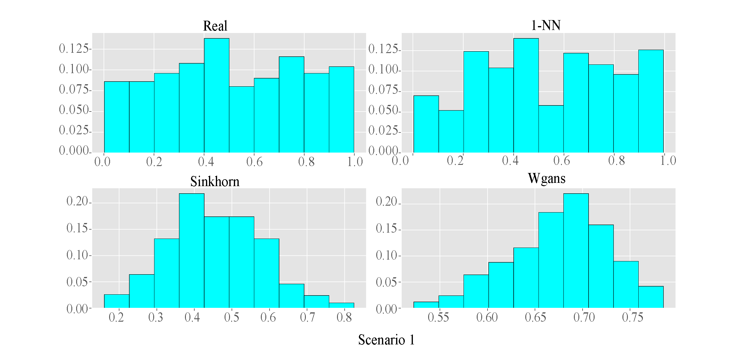
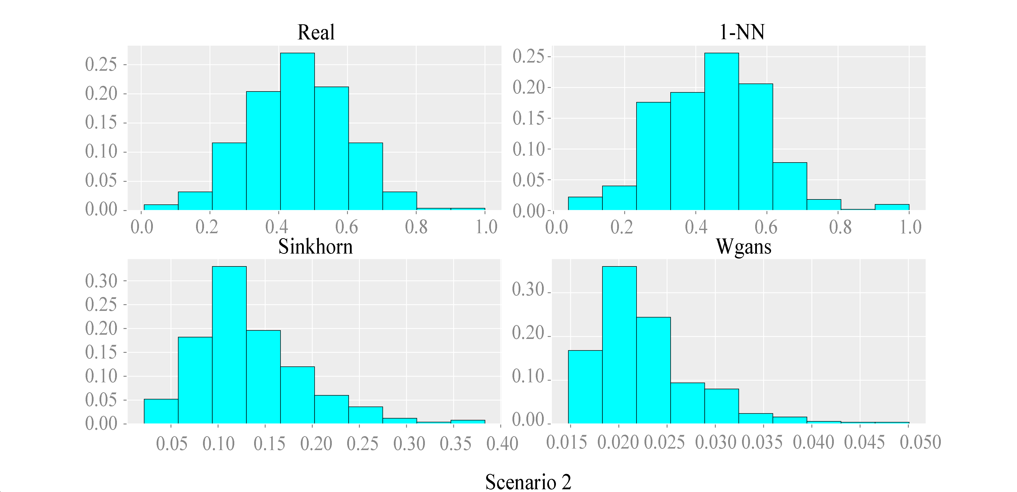
Figure 1: The conditional histograms.

Nearest-Neighbor Sampling Based CIT

In this section, we introduce our CIT based on the nearest-neighbor sampling (NNSCIT) and present the pseudo code of computing NNSCIT and its $p$-value in Algorithm 2. Moreover, theoretically, we show that our proposed test achieves a valid control of the type-I error.

The Proposed CIT Approach

Our CIT test is based on an approximation of CMI $I(X;Y|Z)=I(X;Y,Z)-I(X;Z)$, where $I(X;Y,Z)$ and $I(X;Z)$ are, respectively, the mutual information of $(X;Y,Z)$ and that of $(X;Z)$. We construct our CIT statistic as a classifier-based CMI estimator (CCMI, Mukherjee, Asnani, and Kannan, 2020) of $I(X;Y|Z)$ given by

$$\widehat{I}(X;Y|Z)=\widehat{I}(X;Y,Z)-\widehat{I}(X;Z),$$ (2)

where $\widehat{I}(X;Y,Z)$ (or $\widehat{I}(X;Z)$) is a classifier-based estimator of $I(X;Y,Z)$ (or $I(X;Z)$). By Theorem 1 in Mukherjee, Asnani, and Kannan (2020), $\widehat{I}(X;Y|Z)$ is a consistent estimator of ${I}(X;Y|Z)$. Furthermore, generate samples $\widetilde{X}^{(m)}$ ($m=1,\ldots,M$) from 1-NN conditioned on $Z$, we can show that $\widehat{I}(\widetilde{X}^{(m)};Y|Z)-{I}(\widetilde{X}^{(m)};Y|Z)$ converges to zero for all $m$.

Without loss of generality, we discuss how to approximate $I(X;Z)=D_{KL}(p_{X,Z}(x,z)||p_{X}(x)p_{Z}(z))$, where $p_{X,Z}(x,z)$ is the joint density of $(X,Z)$ and $p_{X}(x)$ and $p_{Z}(z)$ are, respectively, the marginal density of $X$ and $Z$. Moreover, $D_{KL}(F||G)=\int f(x)\log(f(x)/{g(x)})dx$ is the Kullback-Leibler (KL) divergence between two distribution functions $F$ and $G$, whose density functions are given by $f(x)$ and $g(x)$, respectively. The Donsker-Varadhan (DV) representation of $D_{KL}(F||G)$ is given by

$$\sup_{s\in\mathcal{S}}\left[E_{x\sim f}s(x)-\log\{E_{x\sim g}\exp(s(x))\}\right],$$ (3)

where the function class $\mathcal{S}$ includes all functions with finite expectations in (3). The optimal function in (3) is given by $s^{*}(x)=\log({f(x)}/{g(x)})$ (Belghazi et al. 2018), leading to

$$D_{KL}(F||G)=E_{x\sim f}\log\left\{\frac{f(x)}{g(x)}\right\}-\log\left[E_{x\sim g}\left\{\frac{f(x)}{g(x)}\right\}\right].$$ (4)

Following Mukherjee, Asnani, and Kannan (2020), we use the classier two-sample principle (Lopez-Paz and Oquab 2017) to estimate the likelihood ratio $L(x)={f(x)}/{g(x)}$ as follows. Specifically, we consider $n$ i.i.d. samples $\{X_{i}^{f}\}_{i=1}^{n}$ with $X_{i}^{f}\sim f(x)$ and $d$ i.i.d. samples $\{X_{j}^{g}\}_{j=1}^{d}$ with $X_{j}^{g}\sim g(x)$. We label $y_{i}^{f}=1$ for all $X_{i}^{f}$ and $y_{j}^{g}=0$ for all $X_{j}^{g}$. One trains a binary classifier using deep neural network on this supervised classification task. The classifier produces predicted probability $\alpha_{l}=Pr(y=1|X_{l})$ for a given sample $X_{l}$, leading to an estimator of the likelihood ratio on $X_{l}$ given by $\widehat{L}(X_{l})={\alpha_{l}}/(1-\alpha_{l})$. Therefore, it follows from (4) that an estimator of the KL-divergence, $\widehat{D}_{KL}(F||G)$, is given by

$${n}^{-1}\sum_{i=1}^{n}\log\widehat{L}(X_{i}^{f})-\log\left\{{d}^{-1}\sum_{j=1}^{d}\widehat{L}(X_{j}^{g})\right\}.$$

Since mutual information is a special case of the KL divergence, we obtain the estimator $\widehat{I}(X;Z)$ of ${I}(X;Z)$ and that of ${I}(X;Y,Z)$.

Following the idea of CRT, the $p$-value of our CIT method can be given by

$$p=\frac{1+\sum_{m=1}^{M}I\left(\widehat{I}(\widetilde{X}^{(m)};Y|Z)\geq\widehat{I}(X;Y|Z)\right)}{1+M}.$$ (5)

In Lemma 3, we show that the excess type I error of the test based on (5) is bounded by the total variation distance between $p_{\bm{X}|\bm{Z}}(\cdot|\bm{Z})$ and $\widehat{p}_{\bm{X}|\bm{Z}}(\cdot|\bm{Z})$. By Theorem 2, we further get $P(p\leq\alpha|H_{0})\leq\alpha+o(1)$. Therefore, the excess type I error of our CIT method is guaranteed to tend to zero as $n\rightarrow\infty$. Two binary classifications based on deep neural network should be trained to get $\widehat{I}(\widetilde{X}^{(m)};Y|Z)$ for each $m$. Together with $\widehat{I}({X};Y|Z)$, $2(M+1)$ binary classification neural networks should be trained for computing the $p$-value in (5). When $M$ is large, the calculation is extremely intensive and time consuming, especially for the case that the dimensionality of $Z$ is high.

In (5), instead of using $\widehat{I}(\widetilde{X}^{(m)};Y|Z)$, we further propose to utilize $\widehat{I}(\widetilde{X}^{(m)};Y)$ calculated by the method of Mesner and Shalizi (2020) according to the following reasons. First, compared with $\widehat{I}(\widetilde{X}^{(m)};Y|Z)$, $\widehat{I}(\widetilde{X}^{(m)};Y)$ is computationally very fast. Second, $\widetilde{X}^{(m)}$ is generated from 1-NN conditional on $Z$, we thus have $I(\widetilde{X}^{(m)};Y|Z)=0$, whereas $\widetilde{X}^{(m)}$ and $Y$ may share information via $Z$, that is, $I(\widetilde{X}^{(m)};Y)\geq I(\widetilde{X}^{(m)};Y|Z)=0$. By the consistency of $\widehat{I}(\widetilde{X}^{(m)};Y|Z)$ and $\widehat{I}(\widetilde{X}^{(m)};Y)$, we conclude that replacing $\widehat{I}(\widetilde{X}^{(m)};Y|Z)$ with $\widehat{I}(\widetilde{X}^{(m)};Y)$ can improve controlling the probability of making type I error of our CIT method. Thus, we propose a simple counterpart of (5) for $p$-value calculation as follows:

$$p=\frac{1+\sum_{m=1}^{M}I\left(\widehat{I}(\widetilde{X}^{(m)};Y)\geq\widehat{I}(X;Y|Z)\right)}{1+M}.$$ (6)

Since $\widetilde{X}^{(m)}_{i}$s are generated by the 1-NN sampling strategy, we call our test as NNSCIT. Equation (6) lays the foundation of our CIT method, whose pseudo code has been summarized in Algorithm 2.

We describe how to obtain $\widehat{I}(\widetilde{X}^{(m)};Y)$. Specifically, given i.i.d. samples $\{(\widetilde{X}_{i},Y_{i})\}_{i=1}^{n}$ with $(\widetilde{X}_{i},Y_{i})\sim p_{\widetilde{X},Y}$. Let $\rho_{k,i}/2$ be the $l_{\infty}$-distance from point $(\widetilde{X}_{i},Y_{i})$ to its $k$th nearest neighbor. Define

$$n_{\widetilde{X},i}=|\{\widetilde{X}_{j}:|\widetilde{X}_{i}-\widetilde{X}_{j}|\leq\rho_{k,i}/2~{},j\neq i\}|,$$

where $|A|$ is the number of elements in the set $A$. Similarly, define $n_{Y,i}$. For each $i$, we define

$$\delta_{i}=\psi(k)-\psi(n_{\widetilde{X},i})-\psi(n_{Y,i})+\psi(n),$$

where $\psi(x):=d\log\Gamma(x)/dx$ is the digamma function. Therefore, we have

$$\widehat{I}(\widetilde{X};Y)=\max\left\{\frac{1}{n}\sum_{i=1}^{n}\delta_{i},0\right\}.$$ (7)

It follows from Theorems 3.1 and 3.2 in Mesner and Shalizi (2020) that $\widehat{I}(\widetilde{X};Y)$ is a consistent estimator of ${I}(\widetilde{X};Y)$.

Finally, we discuss why we cannot replace $\widehat{I}(X;Y|Z)$ by $\widehat{I}(X;Y)$ in (6). One may think of approximating $p$-value as follows:

$$p=\frac{1+\sum_{m=1}^{M}I\left\{\widehat{I}(\widetilde{X}^{(m)};Y)\geq\widehat{I}(X;Y)\right\}}{1+M},$$ (8)

which results in another CRT test. Let $\widehat{c}_{\alpha}$ be the upper $\alpha$ quantile of the distribution of $\widehat{I}(\widetilde{X}^{(m)};Y)$. Given significance level $\alpha$, the rejection regions of (6) and (8) are given by $\{\widehat{I}(X;Y|Z)>\widehat{c}_{\alpha}\}$ and $\{\widehat{I}(X;Y)>\widehat{c}_{\alpha}\}$, respectively. Under $H_{1}$, $I(X;Y|Z)$ should deviate from zero. Intuitively, the test with rejection region $\{\widehat{I}(X;Y|Z)>\widehat{c}_{\alpha}\}$ is more likely to accept $H_{1}$ than that with $\{\widehat{I}(X;Y)>\widehat{c}_{\alpha}\}$. For example, consider $X\rightarrow Z\leftarrow Y$. This relation indicates $X\not\!\perp\!\!\!\perp Y|Z$ ($H_{1}$ holds), but $X$ and $Y$ may be independent. Therefore, the rejection region $\{\widehat{I}(X;Y|Z)>\widehat{c}_{\alpha}\}$ could detect $H_{1}$, but $\{\widehat{I}(X;Y)>\widehat{c}_{\alpha}\}$ may fail to do so. That is, the test using (6) is generally more powerful than that using (8) under $H_{1}$. Consider another special case when $X\perp\!\!\!\perp Z$, we obtain $I(X;Y|Z)\geq I(X;Y)$. By the consistency of $\widehat{I}(X;Y|Z)$ and $\widehat{I}(X;Y)$, replacing $\widehat{I}(X;Y)$ in (8) with $\widehat{I}(X;Y|Z)$ will increase the power under $H_{1}$. That is, (6) endows more power than (8) under $H_{1}$. We can reach the same conclusion for $Y\perp\!\!\!\perp Z$.

Algorithm 2 Nearest-Neighbor sampling based conditional independence test (NNSCIT)

Input: Data-set $U$ of $n$ i.i.d. samples from $p_{X,Y,Z}$.
Parameter: The number of repetitions $M$; the neighbor order $k$ in MI estimation; the significance level $\alpha$.
Output: Accept $H_{0}:X\perp\!\!\!\perp Y|Z$ or $H_{1}:X\not\!\perp\!\!\!\perp Y|Z$.

1:  Randomly divide $U$ into two disjoint parts: $U_{1}:=\{X_{train},Y_{train},Z_{train}\}$ with sample size $n-\lfloor n/3\rfloor$ and $U_{2}:=\{X_{test},Y_{test},Z_{test}\}$ with sample size $\lfloor n/3\rfloor$.

2:  $m=1$.

3:  while $m\leq M$ do

4:     Randomly taking $\lfloor n/3\rfloor$ samples from $U_{1}$ to obtain $V_{1}$.

5:     Produce $U_{0}^{m}:=\{\widetilde{X}^{(m)}\}$ using 1-NN($V_{1}$,$U_{2}$, $\lfloor n/3\rfloor$) in Algorithm 1.

6:     Compute $I^{(m)}:=\widehat{I}(\{\widetilde{X}^{(m)}\};\{Y_{test}\})$ according to Equ. (7).

7:     $m=m+1$.

8:  end while

9:  Compute $I:=\widehat{I}(\{X_{test}\};\{Y_{test}\}|\{Z_{test}\})$ according to Equ. (2).

10:  Compute $p$-value: $p:=\frac{1+\sum_{m=1}^{M}I\{I^{(m)}\geq I\}}{1+M}$.

11:  if $p\geq\alpha$ then

12:     Accept $H_{0}:X\perp\!\!\!\perp Y|Z$.

13:  else

14:     Accept $H_{1}:X\not\!\perp\!\!\!\perp Y|Z$.

15:  end if

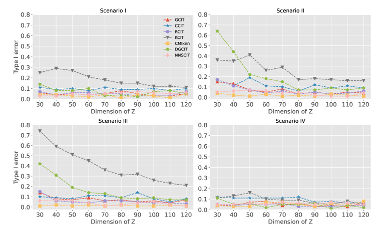
Figure 2: The empirical type-I error rate of various tests under $H_{0}$.

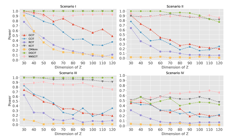
Figure 3: The empirical power of various tests under $H_{1}$.

$d_{Z}$	GCIT	CCIT	RCIT	KCIT	CMIknn	DGCIT	NNSCIT
5	0.11	0.36	0.53	0.72	0.03	0.50	0.01
10	0.48	0.22	0.82	0.84	0.06	0.86	0.05
15	0.87	0.21	0.85	0.93	0.15	0.91	0.05
20	0.93	0.25	0.90	0.98	0.05	0.97	0.07

Table 1: The empirical type-I error rate of various tests for Example 1.

$d_{Z}$	GCIT	CCIT	RCIT	KCIT	CMIknn	DGCIT	NNSCIT
5	0.37	1	0.03	0.02	1	0.78	1
10	0.53	1	0.04	0.10	1	0.82	1
15	0.55	1	0.05	0.14	1	0.79	1
20	0.63	1	0.07	0.16	1	0.88	1

Table 2: The empirical power of various tests for Example 2.

Theoretical Results

In this subsection, we present theoretical results of our NNSCIT based on (5) and (6). We introduce the following notation. Without loss of generality, let $U_{2}:=\{(X_{1},Y_{1},Z_{1}),\ldots,(X_{n_{1}},Y_{n_{1}},Z_{n_{1}})\}$ in Algorithm 2 with $n_{1}=\lfloor n/3\rfloor$, where $\lfloor x\rfloor$ is the largest integer not greater than $x$. We define $\bm{X}:=(X_{1},X_{2},\ldots,X_{n_{1}})$, $\bm{Y}:=(Y_{1},Y_{2},\ldots,Y_{n_{1}})$, and $\bm{Z}:=(Z_{1},Z_{2},\ldots,Z_{n_{1}})$. Denote ${P}(\cdot|\bm{Z}):={p}(\cdot|Z_{1})\times\ldots\times{p}(\cdot|Z_{n_{1}})$ and $\widehat{P}(\cdot|\bm{Z}):=\widehat{p}(\cdot|Z_{1})\times\ldots\times\widehat{p}(\cdot|Z_{n_{1}})$. Assume that $\widetilde{\bm{X}}^{(m)}:=(\widetilde{X}_{1}^{(m)},\ldots,\widetilde{X}_{n_{1}}^{(m)})$ is sampled according to $\widehat{P}(\cdot|\bm{Z})$ for $m=1,\ldots,M$. Let $T(\bm{X},\bm{Y},\bm{Z}):=\widehat{I}(X;Y|Z)$ and $T(\bm{\widetilde{}}{\bm{X}}^{(1)},\bm{Y},\bm{Z}):=\widehat{I}(\widetilde{X}^{(1)};Y|Z),\ldots,$ $T(\bm{\widetilde{}}{\bm{X}}^{(M)},\bm{Y},\bm{Z}):=\widehat{I}(\widetilde{X}^{(M)};Y|Z)$.

Let $\widetilde{\bm{X}}_{F}$ be an additional copy sampled from $\widehat{P}(\cdot|\bm{Z})$ and independently of $\bm{Y}$ and of $\bm{X},\widetilde{\bm{X}}^{(1)},\ldots,\widetilde{\bm{X}}^{(M)}$. Under $H_{0}$: $X\perp\!\!\!\perp Y|Z$, conditionally on $\bm{Y}$ and $\bm{Z}$, $\bm{X}$ and $(\widetilde{\bm{X}}^{(1)},\ldots,\widetilde{\bm{X}}^{(M)})$ are independent, and $\widetilde{\bm{X}}_{F}$ and $(\widetilde{\bm{X}}^{(1)},\ldots,\widetilde{\bm{X}}^{(M)})$ are independent. Thus, we have

$$d_{TV}\{(({\bm{X}},\widetilde{\bm{X}}^{(1)},\ldots,\widetilde{\bm{X}}^{(M)})|\bm{Y},\bm{Z}),$$

$$~{}~{}~{}~{}~{}~{}~{}~{}((\widetilde{\bm{X}}_{F},\widetilde{\bm{X}}^{(1)},\ldots,\widetilde{\bm{X}}^{(M)})|\bm{Y},\bm{Z})\}$$

$$=d_{TV}\{({\bm{X}}|\bm{Y},\bm{Z}),(\widetilde{\bm{X}}_{F}|\bm{Y},\bm{Z})\}=d_{TV}\{P(\cdot|\bm{Z}),\widehat{P}(\cdot|\bm{Z})\}.$$

Define a set $\mathcal{A}_{\alpha}$ as

$$\mathcal{A}_{\alpha}:= \Big{\{}(\bm{x},\widetilde{\bm{x}}^{(1)},\ldots,\widetilde{\bm{x}}^{(M)}):$$

$$\frac{1+\sum_{m=1}^{M}I\{T(\widetilde{\bm{x}}^{(m)},\bm{Y},\bm{Z})\geq T(\bm{x},\bm{Y},\bm{Z})\}}{1+M}\leq\alpha\Big{\}}.$$

Then, we have

$$P(p\leq\alpha|\bm{Y},\bm{Z})=P\{({\bm{X}},\widetilde{\bm{X}}^{(1)},\ldots,\widetilde{\bm{X}}^{(M)})\in\mathcal{A}_{\alpha}|\bm{Y},\bm{Z}\}$$

$$\leq d_{TV}\{(({\bm{X}},\widetilde{\bm{X}}^{(1)},\ldots,\widetilde{\bm{X}}^{(M)})|\bm{Y},\bm{Z}),$$

$$~{}~{}~{}~{}~{}~{}~{}~{}~{}~{}~{}~{}~{}~{}~{}~{}((\widetilde{\bm{X}}_{F},\widetilde{\bm{X}}^{(1)},\ldots,\widetilde{\bm{X}}^{(M)})|\bm{Y},\bm{Z})\}$$

$$~{}~{}+P\{(\widetilde{\bm{X}}_{F},\widetilde{\bm{X}}^{(1)},\ldots,\widetilde{X}^{(M)})\in\mathcal{A}_{\alpha}|\bm{Y},\bm{Z}\}$$

$$=d_{TV}\{P(\cdot|\bm{Z}),\widehat{P}(\cdot|\bm{Z})\}$$

$$~{}~{}+P\{(\widetilde{\bm{X}}_{F},\widetilde{\bm{X}}^{(1)},\ldots,\widetilde{\bm{X}}^{(M)})\in\mathcal{A}_{\alpha}|\bm{Y},\bm{Z}\}.$$

Conditioning on $\bm{Y}$ and $\bm{Z}$, $\widetilde{\bm{X}}_{F},\widetilde{\bm{X}}^{(1)},\ldots,\widetilde{\bm{X}}^{(M)}$ are identically distributed and thus exchangeable, so $P\{(\widetilde{\bm{X}}_{F},\widetilde{\bm{X}}^{(1)},\ldots,\widetilde{\bm{X}}^{(M)})\in\mathcal{A}_{\alpha}|\bm{Y},\bm{Z}\}\leq\alpha$ holds and we obtain the following result.

Lemma 3.

Assume that $H_{0}:X\perp\!\!\!\perp Y|Z$ is true, for any desired significance level $\alpha\in(0,1)$, the type I error of test (5) satisfies

$$P(p\leq\alpha|\bm{Y},\bm{Z})\leq\alpha+d_{TV}\{P(\cdot|\bm{Z}),\widehat{P}(\cdot|\bm{Z})\}.$$ (9)

An immediate implication of Lemma 3 is that the type I error rate holds unconditionally as follows:

$$P(p\leq\alpha|H_{0})\leq\alpha+E[d_{TV}\{P(\cdot|\bm{Z}),\widehat{P}(\cdot|\bm{Z})\}].$$

Furthermore, for any given test statistic $T(\cdots)$, we can compute the $p$-value via (1) by replacing $\bm{X}^{(m)}$ with the 1-NN sample $\widetilde{\bm{X}}^{(m)}$. The resulting test also enjoys (9) by similar arguments.

Under $H_{0}$, $I(\widetilde{X}^{(m)};Y)\geq I(\widetilde{X}^{(m)};Y|Z)$. Denote the $p$ values in (5) and (6) as $p$ and $p^{*}$, respectively. With the consistency of $\widehat{I}(\widetilde{X}^{(m)};Y|Z)$ and $\widehat{I}(\widetilde{X}^{(m)};Y)$, we obtain the following main result.

Theorem 4.

Assume that $H_{0}$ holds, we have

$$P(p^{*}\leq\alpha|H_{0})-\alpha \leq P(p\leq\alpha|H_{0})-\alpha$$

$$\leq E[d_{TV}\{P(\cdot|\bm{Z}),\widehat{P}(\cdot|\bm{Z})\}].$$

Theorem 4 has three important implications. First, the excess type I error over a desired level $\alpha\in(0,1)$ of the test (6) is bounded by $E\{d_{TV}(\widehat{P}(\cdot|\bm{Z}),P(\cdot|\bm{Z}))\}$. Second, our proposed method outperforms CRT (5) in controlling type I error. Third, by Theorem 2, we get

$$P(p^{*}\leq\alpha|H_{0})\leq\alpha+o(1).$$

Thus, the excess type I error of our NNSCIT is guaranteed to be small.

Performance Evaluation

In this section, we examine the finite sample performance of our NNSCIT by using the synthetic datasets. We compare NNSCIT with GCIT (Bellot and van der Schaar 2019), the classifier-based CI test (CCIT) (Sen et al. 2017), the kernel-based CI test (KCIT) (Zhang et al. 2011), RCIT (Strobl, Zhang, and Visweswaran 2019), the CMI-based CI test (CMIknn) (Runge 2018), and DGCIT (Shi et al. 2021). We leave some additional simulation studies and the real data analysis in the Supplementary Materials. The source code of NNSCIT is available at https://github.com/LeeShuai-kenwitch/NNSCIT.

Performances on Synthetic Dataset

The synthetic data sets are generated by using the post non-linear model similar to those in Zhang et al. (2011); Doran et al. (2014); and Bellot and van der Schaar (2019). Specifically, we define $(X,Y,Z)$ under $H_{0}$ and $H_{1}$ as follows:

$$H_{0}:X=f(A_{f}^{T}Z+\epsilon_{f}),~{}Y=g(A_{g}^{T}Z+\epsilon_{g}),$$

$$H_{1}:Y=h(A_{h}^{T}Z+bX)+\epsilon_{h}.$$

The entries of $A_{f}$ and $A_{g}$ are randomly and uniformly sampled from $[0,1]$ and then normalized to the unit $l_{1}$ norm. The entries of $A_{h}$ are sampled from a standard normal distribution and $b$ is set to $2$. The noise variables $\epsilon_{f}$, $\epsilon_{g}$ and $\epsilon_{h}$ are independently sampled from a normal distribution with mean zero and variance 0.49. The significance level is set at $\alpha=0.05$ and the sample size is fixed at $n=1000$. Set $M=500$ and $k=3$. Consider the following four scenarios:

Scenario I. Set $f$, $g$ and $h$ to be the identity functions, inducing linear dependencies, $Z\sim N(0.7,1)$, and $X\sim N(0,1)$ under $H_{1}$.

Scenario II. Set $f$, $g$ and $h$ as in Scenario I, but use a Laplace distribution to generate $Z$.

Scenario III. Set $f$, $g$ and $h$ as in Scenario I, but use Uniform$[-2.5,2.5]$ to generate $Z$.

Scenario IV. Set $f$, $g$ and $h$ to be randomly sampled from $\left\{x^{2},x^{3},\mbox{tanh}(x),\cos(x)\right\}$. Set $Z\sim N(0,1)$, and $X\sim N(0,1)$ under $H_{1}$.

We vary the dimension of $Z$ as $d_{Z}=30,$ $40,$ $50,$ $60,$ $70,$ $80,$ $90,$ $100,$ $110,$ and $120$. Figures 2 and 3 include the type-I error rates under $H_{0}$ and powers under $H_{1}$, respectively, over $300$ data replications. Additional simulation results for $d_{Z}=5,10,15,20,$ and $25$ can be found in the Supplementary Materials (Figures 1 and 2).

We have the following observations. First, our test controls type I error very well under $H_{0}$, while achieves high power under $H_{1}$. Second, CMIknn has satisfactory performances in controlling type-I error, but under $H_{1}$, it loses power in almost all scenarios. Third, although DGCIT and KCIT have adequate power under $H_{1}$, they have inflated type-I errors in some cases, especially when $d_{Z}$ is less than $30$. Fourth, GCIT, CCIT and RCIT cannot control type-I errors in some cases, especially when $d_{Z}$ is less than $30$. Moreover, under $H_{1}$, GCIT, CCIT and RCIT lose some power in almost all scenarios.

Figure 4 in the Supplementary Materials reports the run times as a function of $d_{Z}$ for a single CIT with data generated under Scenario II. Other scenarios show similar performance. Our NNSCIT is computationally very efficient. In contrast, CCIT, CMIknn and DGCIT are very time-consuming and are prohibitive in practice.

Performances on Two Examples

As discussed in the Introduction, we evaluate the performances of our method in the following two examples. The details of data generation mechanisms are presented in the Supplementary Materials.

Example 1. $X\rightarrow Z\rightarrow Y$. In this case, $H_{0}$ holds, but there is a strong dependence between $X$ and $Y$. Table 1 reports the type-I error rates. Our NNSCIT controls type-I error very well, but GCIT, CCIT, RCIT, KCIT and DGCIT break down as their type-I errors are very large.

Example 2. $X\rightarrow Z\leftarrow Y$. In this case, $H_{1}$ holds, but $X$ and $Y$ are independent. Table 2 reports the powers of different methods. Our method achieves power as high as $1$. In contrast, RCIT and KCIT have power less than $0.2$ and GCIT and DGCIT also lose some power.

Conclusion

In this paper, we propose a novel and fast NNSCIT. We use the 1-NN sampling strategy to approximate the conditional distribution $X|Z$. Compared with GANs, 1-NN not only has computational efficiency, but also exhibits advantage in approximation accuracy. We take the classifier-based conditional mutual information (CCMI) estimator as our test statistic, which captures the conditional-dependence feature very well. We show that our NNSCIT has three notable features, including controlling type-I error well, achieving high power under $H_{1}$, and being computationally efficient.

References

- Arjovsky, Chintala, and Bottou (2017) Arjovsky, M.; Chintala, S.; and Bottou, L. 2017. Wasserstein generative adversarial networks. In International Conference on Machine Learning, 214–223. PMLR.
- Belghazi et al. (2018) Belghazi, M. I.; Baratin, A.; Rajeshwar, S.; Ozair, S.; Bengio, Y.; Courville, A.; and Hjelm, D. 2018. Mutual information neural estimation. In International Conference on Machine Learning, 531–540. PMLR.
- Bellot and van der Schaar (2019) Bellot, A.; and van der Schaar, M. 2019. Conditional independence testing using generative adversarial networks. In Advances in Neural Information Processing Systems, 2199–2208.
- Berrett et al. (2020) Berrett, T. B.; Wang, Y.; Barber, R. F.; and Samworth, R. J. 2020. The conditional permutation test for independence while controlling for confounders. Journal of the Royal Statistical Society: Series B (Statistical Methodology), 82(1): 175–197.
- Cai, Li, and Zhang (2022) Cai, Z.; Li, R.; and Zhang, Y. 2022. A distribution free conditional independence test with applications to causal discovery. Journal of Machine Learning Research, 23(85): 1–41.
- Candes et al. (2018) Candes, E.; Fan, Y.; Janson, L.; and Lv, J. 2018. Panning for gold:‘model-X’ knockoffs for high dimensional controlled variable selection. Journal of the Royal Statistical Society: Series B (Statistical Methodology), 80(3): 551–577.
- Cover and Hart (1967) Cover, T.; and Hart, P. 1967. Nearest neighbor pattern classification. IEEE Transactions on Information Theory, 13(1): 21–27.
- Cover and Thomas (2012) Cover, T. M.; and Thomas, J. A. 2012. Elements of Information Theory. John Wiley & Sons.
- Devroye et al. (1994) Devroye, L.; Gyorfi, L.; Krzyzak, A.; and Lugosi, G. 1994. On the strong universal consistency of nearest neighbor regression function estimates. The Annals of Statistics, 22(3): 1371–1385.
- Doran et al. (2014) Doran, G.; Muandet, K.; Zhang, K.; and Schölkopf, B. 2014. A Permutation-Based Kernel Conditional Independence Test. In Uncertainty in Artificial Intelligence, 132–141. Citeseer.
- Fix and Hodges (1951) Fix, E.; and Hodges, J. L. 1951. Discriminatory Analysis, Nonparametric Discrimination: Consistency Properties. Technical Report 4, USAF School of Aviation Medicine.
- Fleuret (2004) Fleuret, F. 2004. Fast binary feature selection with conditional mutual information. Journal of Machine Learning Research, 5(9): 1531–1555.
- Gao, Oh, and Viswanath (2016) Gao, W.; Oh, S.; and Viswanath, P. 2016. Breaking the bandwidth barrier: Geometrical adaptive entropy estimation. In Advances in Neural Information Processing Systems, 2460–2468.
- Gao, Oh, and Viswanath (2017) Gao, W.; Oh, S.; and Viswanath, P. 2017. Demystifying fixed k-nearest neighbor information estimators. In IEEE International Symposium on Information Theory, 1267–1271.
- Genevay, Peyré, and Cuturi (2018) Genevay, A.; Peyré, G.; and Cuturi, M. 2018. Learning generative models with sinkhorn divergences. In International Conference on Artificial Intelligence and Statistics, 1608–1617. PMLR.
- Hlinka et al. (2013) Hlinka, J.; Hartman, D.; Vejmelka, M.; Runge, J.; Marwan, N.; Kurths, J.; and Paluš, M. 2013. Reliability of inference of directed climate networks using conditional mutual information. Entropy, 15(6): 2023–2045.
- Koller and Friedman (2009) Koller, D.; and Friedman, N. 2009. Probabilistic graphical models: principles and techniques. MIT press.
- Lauritzen (1996) Lauritzen, S. L. 1996. Graphical models, volume 17. Clarendon Press.
- Liang and Wang (2008) Liang, K.-C.; and Wang, X. 2008. Gene regulatory network reconstruction using conditional mutual information. EURASIP Journal on Bioinformatics and Systems Biology, 2008: 1–14.
- Lopez-Paz and Oquab (2017) Lopez-Paz, D.; and Oquab, M. 2017. Revisiting classifier two-sample tests. In International Conference on Learning Representations.
- Mesner and Shalizi (2020) Mesner, O. C.; and Shalizi, C. R. 2020. Conditional mutual information estimation for mixed, discrete and continuous data. IEEE Transactions on Information Theory, 67(1): 464–484.
- Mukherjee, Asnani, and Kannan (2020) Mukherjee, S.; Asnani, H.; and Kannan, S. 2020. CCMI: Classifier based conditional mutual information estimation. In Uncertainty in Artificial Intelligence, 1083–1093. PMLR.
- Pearl (2009) Pearl, J. 2009. Causality. Cambridge university press.
- Runge (2018) Runge, J. 2018. Conditional independence testing based on a nearest-neighbor estimator of conditional mutual information. In International Conference on Artificial Intelligence and Statistics, 938–947. PMLR.
- Sen et al. (2017) Sen, R.; Suresh, A. T.; Shanmugam, K.; Dimakis, A. G.; and Shakkottai, S. 2017. Model-powered conditional independence test. In Advances in Neural Information Processing Systems, 2955–2965.
- Shah and Peters (2020) Shah, R. D.; and Peters, J. 2020. The hardness of conditional independence testing and the generalised covariance measure. The Annals of Statistics, 48(3): 1514–1538.
- Shi et al. (2021) Shi, C.; Xu, T.; Bergsma, W.; and Li, L. 2021. Double generative adversarial networks for conditional independence testing. Journal of Machine Learning Research, 22(285): 1–32.
- Silverman (2018) Silverman, B. W. 2018. Density estimation for statistics and data analysis. Routledge.
- Spirtes et al. (2000) Spirtes, P.; Glymour, C. N.; Scheines, R.; and Heckerman, D. 2000. Causation, prediction, and search. MIT press.
- Strobl, Zhang, and Visweswaran (2019) Strobl, E. V.; Zhang, K.; and Visweswaran, S. 2019. Approximate kernel-based conditional independence tests for fast non-parametric causal discovery. Journal of Causal Inference, 7(1): 1–24.
- Zhang et al. (2017) Zhang, H.; Zhou, S.; Zhang, K.; and Guan, J. 2017. Causal discovery using regression-based conditional independence tests. In Proceedings of the AAAI Conference on Artificial Intelligence, 1250–1256.
- Zhang et al. (2022) Zhang, H.; Zhou, S.; Zhang, K.; and Guan, J. 2022. Residual similarity based conditional independence test and its application in causal discovery. In Proceedings of the AAAI Conference on Artificial Intelligence, 5942–5949.
- Zhang et al. (2011) Zhang, K.; Peters, J.; Janzing, D.; and Schölkopf, B. 2011. Kernel-based conditional independence test and application in causal discovery. In Proceedings of the Twenty-Seventh Conference on Uncertainty in Artificial Intelligence, 804–813.