Neural network assisted quantum state and process tomography using limited data sets

Abstract

In this study we employ a feed-forward artificial neural network (FFNN) architecture to perform tomography of quantum states and processes obtained from noisy experimental data. To evaluate the performance of the FFNN, we use a heavily reduced data set and show that the density and process matrices of unknown quantum states and processes can be reconstructed with high fidelity. We use the FFNN model to tomograph 100 two-qubit and 128 three-qubit states which were experimentally generated on a nuclear magnetic resonance (NMR) quantum processor. The FFNN model is further used to characterize different quantum processes including two-qubit entangling gates, a shaped pulsed field gradient, intrinsic decoherence processes present in an NMR system, and various two-qubit noise channels (correlated bit flip, correlated phase flip and a combined bit and phase flip). The results obtained via the FFNN model are compared with standard quantum state and process tomography methods and the computed fidelities demonstrates that for all cases, the FFNN model outperforms the standard methods for tomography.

I Introduction

Quantum state tomography (QST) and quantum process tomography (QPT) are essential techniques to characterize unknown quantum states and processes respectively, and to evaluate the quality of quantum devices Nielsen and Chuang (2010); Childs et al. (2001); O${}^{{}^{\prime}}$Brien et al. (2004). Numerous computationally and experimentally efficient QST and QPT algorithms have been designed such as self-guided tomographyChapman et al. (2016), adaptive tomography Pogorelov et al. (2017), compressed sensing based QST and QPT protocols which use heavily reduced data sets Riofrao et al. (2017); Gaikwad et al. (2021), selective QPT Bendersky et al. (2008); Gaikwad et al. (2018, 2022), and direct QST/QPT using weak measurements Kim et al. (2018).

Recently, machine learning (ML) techniques have been used to improve the efficiency of tomography protocols Carleo and Troyer (2017); Carleo et al. (2019); Torlai and Melko (2020). QST was performed on entangled quantum states using a restricted Boltzmann machine based artificial neural network (ANN) model Torlai et al. (2018) and was experimentally implemented on an optical system Neugebauer et al. (2020). ML based adaptive QST was performed which adapts to experiments and suggests suitable further measurements Quek et al. (2021). QST using an attention based generative network was realized experimentally on an IBMQ quantum computerCha et al. (2021). ANN enhanced QST was carried out after minimizing state preparation and measurement errors when reconstructing the state on a photonic quantum dataset Palmieri et al. (2020a). A convolutional ANN model was employed to reconstruct quantum states with tomography measurements in the presence of simulated noise Lohani et al. (2020). Local measurement-based QST via ANN was experimentally demonstrated on NMRXin et al. (2019). ML was used to detect experimental multipartite entanglement structure for NMR entangled states Tian et al. (2022). ANN was used to perform QST while taking into account measurement imperfections Pan and Zhang (2022) and were trained to uniquely reconstruct a quantum state without requiring any prior information about the state Teo et al. (2021). ANN was used to reconstruct quantum states encoded in the spatial degrees of freedom of photons with high fidelity Palmieri et al. (2020b). ML methods were used to directly estimate the fidelity of prepared quantum states Zhang et al. (2021). ANN was used to reconstruct quantum states in the presence of various types of noise Koutny et al. (2022). Quantum state tomography in intermediate-scale quantum devices was performed using conditional generative adversial networks Ahmed et al. (2021).

In this study, we employed a Feed Forward Neural Network (FFNN) architecture to perform quantum state as well as process tomography. We trained and tested the model on states/processes generated computationally and then validated it on noisy experimental data generated on an NMR quantum processor. Furthermore, we tested the efficacy of the FFNN model on a heavily reduced data set, where a random fraction of the total data set was used. The FFNN model was able to reconstruct the true quantum states and quantum processes with high fidelity even with this heavily reduced data set.

This paper is organized as follows: Section II briefly describes the basic framework of the FFNN model in the context of QST and QPT; Section II.1 describes the FFNN architecture while Section II.2 details how to construct the FFNN training data set to perform QST and QPT. Sections III and IV contain the results of implementing the FFNN to perform QST and QPT of experimental NMR data, respectively. Section V contains a few concluding remarks.

II FFNN Based QST and QPT

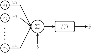
Figure 1: (Color online) Basic unit of an ANN model, where the $x_{i}$ are the inputs, $w_{i}$ are the weights, $b$ is the bias, $\sum$ is the summation function, $f$ is an activation function and $\tilde{y}$ is the output of the ANN.

II.1 The Basic FFNN Architecture

First we describe the multilayer perceptron model also referred to as a Feed-Forward-Neural network (FFNN) which we employ to the task of characterizing quantum states and processes. An ANN is a mathematical computing model motivated by the biological nervous system which consists of adaptive units called neurons which are connected to other neurons via weights. A neuron is activated when its value is greater than a ‘threshold value’ termed the bias. Figure 1 depicts a schematic of an ANN with $n$ inputs $x_{1},x_{2},\cdots,x_{n}$ which are connected to a neuron with weights $w_{1},w_{2},\cdots,w_{n}$; the weighted sum of these inputs is compared with the bias $b$ and is acted upon the activation function $f$, with the output $\tilde{y}=f(\sum_{i=1}^{n}w_{i}x_{i}-b)$.

A multilayer FFNN architecture consists of three layers: the input layer, the hidden layer and the output layer. Data is fed into the input layer, which is passed on to the hidden layers and finally from the last hidden layer, it arrives at the output layer. Figure 2 depicts a schematic of a prototypical FFNN model with one input layer, two hidden layers and one output layer, which has been employed (as an illustration) to perform QST of an experimental two-qubit NMR quantum state, using a heavily reduced data set.

The data is divided into two parts: a training dataset which is used to train the model, a process in which network parameters, (weights and biases) are updated based on the outcomes and a test dataset which is used to evaluate the network performance. Consider ‘$m$’ training elements $\{(\vec{x}^{(1)},\vec{y}^{(1)}),(\vec{x}^{(2)},\vec{y}^{(2)}),\cdots,(\vec{x}^{(p)},\vec{y}^{(p)})\}$ where $\vec{x}^{(i)}$ is the $i^{th}$ input and $\vec{y}^{(i)}$ is the corresponding output. Feeding these inputs to the network produces the outputs $[\tilde{\vec{y}}^{(1)},\tilde{\vec{y}}^{(2)},...,\tilde{\vec{y}}^{(p)}]$. Since network parameters are initialized randomly, the predicted output is not equal to the expected output. Training of this network can be achieved by minimizing a mean-squared-error cost function, with respect to the network parameters, by using a stochastic gradient descent method and the backpropagation algorithm Ruder (2017):

$$w_{ij}\rightarrow w^{\prime}_{ij}= w_{ij}-\frac{\eta}{p^{\prime}}\sum_{i=1}^{p^{\prime}}\frac{\partial}{\partial w_{ij}}\mathcal{L}(\vec{x}^{(i)})$$ (1)

$$b_{i}\rightarrow b^{\prime}_{i}= b_{i}-\frac{\eta}{p^{\prime}}\sum_{i=1}^{p^{\prime}}\frac{\partial}{\partial b_{i}}\mathcal{L}(\vec{x}^{(i)})$$ (2)

where $\mathcal{L}(x^{(i)})=||\vec{y}^{(i)}-\tilde{\vec{y}}^{(i)}||^{2}$ is the cost function of the randomly chosen $m^{\prime}$ training inputs $x^{(i)}$, $\eta$ is the learning rate and $w^{\prime}_{ij}$ and $b^{\prime}_{i}$ are updated weights and biases, respectively.

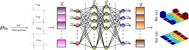
Figure 2: (Color online) Flowchart illustrating the FFNN model used to perform QST on two-qubit quantum states generated on an NMR quantum; on the left, $\rho_{in}$ represents the state which is to be tomographed; ${\rm IY}$ denotes a tomographic operation, which is followed by signal detection, the set of depicted NMR spectra are those obtained after the tomographic measurement. The FFNN with two hidden layers is represented next, which then uses a reduced data set to reconstruct the final experimental tomographs represented on the right.

II.2 FFNN Training Dataset for QST and QPT

An $n$-qubit density operator $\rho$ can be expressed as a matrix in the product basis by:

$$\rho=\sum_{i=0}^{3}\sum_{j=0}^{3}...\sum_{n=0}^{3}a_{ij...n}\sigma_{i}\otimes\sigma_{j}\otimes...\sigma_{n}$$ (3)

where $a_{00...0}=1/2^{n}$, $\sigma_{0}$ denotes the $2\times 2$ identity matrix and $\sigma_{i},i=1,2,3$ are single-qubit Pauli matrices.

The aim of QST is to reconstruct $\rho$ from a set of tomographic measurements. The standard procedure for QST involves solving linear system of equations of the form Long et al. (2001):

$$\mathcal{A}\mathcal{X}=\mathcal{B}$$ (4)

where $\mathcal{A}$ is a fixed coefficient matrix and only depends on the chosen measurement settings, $\mathcal{X}$ is a column matrix which contains elements of the density matrix which needs to be reconstructed, and the input vector $\mathcal{B}$ contains the actual experimental data.

The FFNN model is trained on a dataset containing randomly generated pure and mixed states. To generate these ensembles, consider a normal distribution $\mathcal{N}(\mu=0,\sigma^{2}=1)$ with zero mean and unit variance. An $n$-qubit pure random state in the computational basis is represented by an $2^{n}$ column vector $C$ whose $i$th entry $c_{i}$ generated from the random distribution as follows:

$$c_{i}=\frac{1}{N}(\mathfrak{d}_{i}+i\,\mathfrak{e}_{i})$$ (5)

where $\mathfrak{d}_{i},\mathfrak{e}_{i}$ are randomly chosen from the distribution $\mathcal{N}$ and $N$ is a normalization factor to ensure that $C$ represent a unit vector.

For mixed states:

$$R=\mathcal{D}_{i}+i\,\mathcal{E}_{i}$$ (6)

where $R$ is a $2^{n}\times 2^{n}$ matrix with its elements $\mathcal{D}_{i},\mathcal{E}_{i}$ randomly sampled from the normal distribution $\mathcal{N}$. Using the $R$ matrix, the corresponding mixed state density matrix $\rho_{\rm{mix}}$ is constructed as $\rho_{\rm{mix}}=\frac{RR^{\dagger}}{\rm{Tr}(RR^{\dagger})}$.

The FFNN is trained on both pure as well as mixed states and the appropriate density matrices are generated. After generating the density matrices $\mathcal{X}_{i}$, the corresponding $\mathcal{B}_{i}$ are computed using Eq.(4). The training elements $\{\mathcal{B}_{i},\mathcal{X}_{i}\}$ are then used to train the FFNN model given in Figure 2, where $\mathcal{B}_{i}$ are the inputs to the FFNN and $\mathcal{X}_{i}$ are the corresponding labeled outputs.

QPT of given a quantum process is typically performed using the Kraus operator representation, wherein for a fixed operator basis set $\{E_{i}\}$, a quantum map $\Lambda$ acting on an input state $\rho_{{\rm in}}$ can be written as Kraus et al. (1983):

$$\Lambda(\rho_{in})=\sum_{m,n}\chi_{mn}E_{m}\rho_{in}E_{n}^{\dagger}$$ (7)

where $\chi_{mn}$ are the elements of the process matrix $\chi$ characterizing the quantum map $\Lambda$. The $\chi$ matrix can be experimentally determined by preparing a complete set of linearly independent input states, estimating the output states after action of the map, and finally computing the elements of $\chi_{mn}$ from these experimentally estimated output states via linear equations of the formChuang and Nielsen (1997):

$$\beta\vec{\chi}=\vec{\lambda}$$ (8)

where $\beta$ is a coefficient matrix, $\vec{\chi}$ contains the elements $\{\chi_{mn}\}$ which are to be determined and $\vec{\lambda}$ is a vector representing the experimental data.

The training data set for using the FFNN model to perform QPT is constructed by randomly generating a set of unitary operators. The generated unitary operators are allowed to act upon the input states $\rho_{in}=\{|0\rangle,|1\rangle,\frac{1}{\sqrt{2}}(|0\rangle+|1\rangle),\frac{1}{\sqrt{2}}(|0\rangle+i|1\rangle)\}^{\otimes n}$, to obtain $\rho_{out}=U\rho_{in}U^{\dagger}$. All the output states $\rho_{out}$ are stacked to form form $\vec{\lambda}$. Finally, $\vec{\chi}$ is computed using Eq. (8). The training elements $\{\vec{\lambda}_{i},\vec{\chi}_{i}\}$ will then be used to train the FFNN model, where $\vec{\lambda}_{i}$ acts as the input to FFNN and $\vec{\chi}_{i}$ is the corresponding labeled output.

Table 1: Average state fidelities obtained after training the FFNN model to perform QST on 3000 test two-qubit states ($M_{{\rm data}}=20$) for training datasets of different sizes, with the number of epochs varying from 50 to 150 for each dataset (an epoch refers to one iteration of the complete training dataset).

Dataset Size	Fidelity
	Epoch(50)	Epoch(100)	Epoch(150)
500	0.8290	0.9176	0.9224
1000	0.9244	0.9287	0.9298
5000	0.9344	0.9379	0.9389
10000	0.9378	0.9390	0.9400
20000	0.9394	0.9414	0.9409
80000	0.9426	0.9429	0.9422

Table 2: Average state fidelities obtained after training the FFNN model to perform QST on 3000 test three-qubit states ($M_{{\rm data}}=120$) for training datasets of different sizes, with the number of epochs varying from 50 to 150 for each dataset (an epoch refers to one iteration of the complete training dataset).

Dataset Size	Fidelity
	Epoch(50)	Epoch(100)	Epoch(150)
500	0.6944	0.8507	0.8716
1000	0.8793	0.8994	0.9025
5000	0.9231	0.9262	0.9285
10000	0.9278	0.9321	0.9332
20000	0.9333	0.9362	0.9393
80000	0.9413	0.9433	0.9432

Table 3: Average process fidelities obtained after training the FFNN model to perform QPT on 3000 test three-qubit states ($M_{{\rm data}}=200$) for training datasets of different sizes, with the number of epochs varying from 50 to 150 for each dataset (an epoch refers to one iteration of the complete training dataset).

Dataset Size	Fidelity
	Epoch(50)	Epoch(100)	Epoch(150)
500	0.4904	0.5421	0.5512
2000	0.6872	0.7090	0.7202
15000	0.7947	0.8128	0.8218
20000	0.8047	0.8203	0.8295
50000	0.8305	0.8482	0.8598
80000	0.8441	0.8617	0.8691

To perform tomography of given state or process one has to perform a series of experiments. Then the input vector is constructed where the entries are outputs/readouts of the experiments. In the case of standard QST or QPT, a tomographically complete set of experiments needs to be done and the input vector corresponding to the tomographically complete set of experiments is referred to as the full data set. To perform QST and QPT via FFNN on a heavily reduced data set of size $m$, a reduced size input vector $\vec{b}_{m}$ with fewer elements (and a correspondingly reduced $\vec{\lambda}_{m}$) is constructed by randomly selecting $m$ elements from the input vectors while the remaining elements are set to 0 (zero padding); these reduced input vectors together with the corresponding labeled output vectors are used to train the FFNN.

The FFNN was trained and implemented using the Keras Python library Chollet (2015) with the Tensor-Flow backend, on an Intel Xeon processor with 48GB RAM and a CPU base speed of 3.90GHz. To perform QST and QPT the LeakyReLU ($\alpha=0.5$) activation function was used for both the input and the hidden layers of the FFNN:

$$\begin{split}\text{LeakyReLU(x)}=&x\,;\,x>0\\ =&\alpha x\,;\,x<0\end{split}$$ (9)

A linear activation function was used for the output layer. A cosine similarity loss function, $\mathcal{L}=\arccos\left(\frac{\hat{\vec{y}}.\tilde{\vec{y}}}{||\hat{\vec{y}}||.||\tilde{\vec{y}}||}\right)$ was used for validation and the adagrad ($\eta=0.5$) optimizer with a learning rate $\eta$, was used to train the network. The adagrad optimizer adapts the learning rate relative to how frequently a parameter gets updated during training.

The FFNN was used to perform QST on 3000 two-qubit and three-qubit test quantum states and to perform QPT on 3000 two-qubit test quantum processes for training datasets of different sizes. The number of epochs were varied from 50 to 150 for each dataset, where an epoch refers to one iteration of the training dataset during the FFNN training process. The computed average fidelities of 3000 two-qubit and three-qubit test quantum states and 3000 two-qubit test quantum processes are shown in Tables 1, 2 and 3, respectively; $M_{{\rm data}}$ refers to the reduced size of the data set. After comparing the effect of training data size, the value of $M_{{\rm data}}$ and the number of epochs, the maximum size of the training data set was chosen to be 80000 and the maximum number of epochs was set to 150 for performing QST and QPT. After 150 training epochs the validation loss function remained constant.

III FFNN Based QST on Experimental Data

We used an NMR quantum processor as the experimental testbed to generate data for the FFNN model. We applied FFNN to perform QST of two-qubit and three-qubit quantum states using a heavily reduced data set of noisy data generated on an NMR quantum processor. The performance of the FFNN was evaluated by computing the average state or average process fidelity. The state fidelity is given by Zhang et al. (2014):

$$\mathcal{F}=\frac{\left|\operatorname{Tr}\left[\rho_{{\rm FFNN}}\rho_{{\rm STD}}^{\dagger}\right]\right|}{\sqrt{\operatorname{Tr}\left[\rho_{{\rm FFNN}}^{\dagger}\rho_{{\rm FFNN}}\right]\operatorname{Tr}\left[\rho_{{\rm STD}}^{\dagger}\rho_{{\rm STD}}\right]}}$$ (10)

where $\rho_{{\rm FFNN}}$ and $\rho_{{\rm STD}}$ are the density matrices obtained via the FFNN and the standard linear inversion method, respectively. The process fidelity can be computed by replacing the $\rho$ in Eq. (10) by $\chi$, where $\chi_{{\rm FFNN}}$ and $\chi_{{\rm STD}}$ are process matrices obtained via the FFNN and standard linear inversion method, respectively.

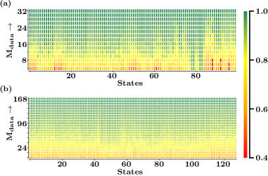
Figure 3: (Color online) Fidelity ($\bar{\mathcal{F}}$) between the FFNN model and the standard linear inversion method vs size of the heavily reduced dataset ($M_{data}$), for QST performed on (a) 100 two-qubit states and (b) 128 three-qubit states respectively. The states are numbered on the $x$-axis and the color coded bar on the right represents the value of the fidelity.

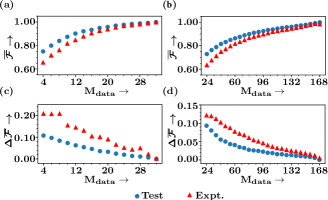
Figure 4: (Color online) Average fidelity ($\bar{\mathcal{F}}$) and standard deviation $\Delta\bar{\mathcal{F}}$ plotted as a function of the size of the heavily reduced dataset ($M_{data}$) computed for FFNN based QST on two qubits ((a) and (c)) and on three qubits ((b) and (d)), respectively. The average fidelity for the test dataset (blue dots) is calculated for 3000 states while for experimental data-set the average fidelity is calculated by randomly choosing the reduced dataset $M_{data}$ elements from the full set for 100 2-qubit states and 128 3-qubit states, and then repeating the procedure 50 times.

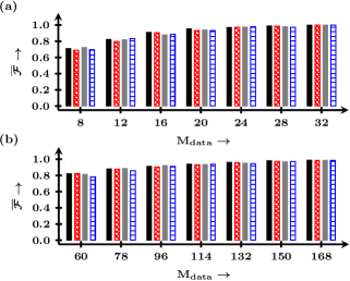
Figure 5: (Color online) Fidelity ($\bar{\mathcal{F}}$) versus size of the heavily reduced dataset ($M_{{\rm data}}$) computed for FFNN based QST of (a) two-qubit Bell states, where the different bars correspond to four different Bell states, and (b) three-qubit GHZ (black and red cross-hatched bars) and Biseparable states (gray and horizontal blue bars).

QST of a two-qubit NMR system is typically performed using a set of four unitary rotations: $\{II,IX,IY,XX\}$ where $I$ denotes the identity operation and $X(Y)$ denotes a $90^{\circ}$ $x$ rotation on the specified qubit. The input vector $\vec{b}$ (Eq. (4)) is constructed by applying the tomographic pulses followed by measurement, wherein the signal which is recorded in the time domain is then Fourier transformed to obtain the NMR spectrum. For two qubits, there are four peaks in the NMR spectrum and each measurement yields eight elements of the vector $\vec{b}$; the dimension of the input vector $\vec{b}$ is $33\times 1$ (32 from tomographic pulses and 1 from the unit trace condition). Similarly, QST of a three-qubit NMR system is typically performed using a set of seven unitary rotations: $\{III,IIY,IYY,YII,XYX,XXY,XXX\}$. Each measurement produces 12 resonance peaks in the NMR spectrum (4 per qubit); the dimension of the input vector $\vec{b}$ is be $169\times 1$. To evaluate the performance of FFNN model in achieving full QST of two-qubit and three-qubit states, we experimentally prepared 100 two-qubit states and 128 three-qubit states using different preparation settings and calculated the average fidelity between the density matrix predicted via the FFNN model and that obtained using the standard linear inversion method for QST. We also performed full FFNN based QST of maximally entangled two-qubit Bell states and three-qubit GHZ and Biseparable states using a heavily reduced data set.

The FFNN model was trained on 80,000 states to perform QST. To perform FFNN based QST on two- and three-qubit states, we used three hidden layers containing 100, 100 and 50 neurons and 300, 200 and 100 neurons, respectively. The performance of the trained FFNN is shown in Figure 3. The fidelity between density matrices obtained via FFNN and standard linear inversion method of 100 experimentally generated two-qubit states and of 128 experimentally generated three-qubit states is shown in Figures 3(a) and (b), respectively. The reduced input vector of size $M_{{\rm data}}$ is plotted on the $y$-axis and the quantum states are numbered along the $x$-axis.

The performance of the FFNN for QST is evaluated in Figure 4 by computing the average state fidelity $\mathcal{\bar{F}}$ calculated over a set of test/experimental states. The reduced size $M_{data}$ of the input vector which was fed into the FFNN is plotted along the $x$-axis. The average fidelity $\mathcal{\bar{F}}$ and the standard deviation $\sigma$ in average state fidelity $\mathcal{\bar{F}}$ are plotted along the $y$-axis in (a) and (c) for two-qubit states and in (b) and (d) for three-qubit states, respectively. For a given value of $M_{data}$, the average fidelity $\mathcal{\bar{F}}_{i}=\frac{1}{50}\sum_{n=1}^{50}\mathcal{F}_{n}$ of a given quantum state $\rho_{i}$ predicted via FFNN is calculated by randomly selecting $M_{data}$ elements from the corresponding full input vector $\vec{b}$ for 50 times. For test data sets (blue circles), the performance of the FFNN is evaluated by computing the average fidelity $\mathcal{\bar{F}}=\frac{1}{3000}\sum_{n=1}^{3000}\mathcal{\bar{F}}_{n}$ over 3000 two-qubit and three-qubit states. For experimental data sets (red triangles), the performance of the FFNN is evaluated by computing the average fidelity $\mathcal{\bar{F}}$ over 100 two-qubit and 128 three-qubit states, respectively. The standard deviation $\sigma$ in average state fidelity $\mathcal{\bar{F}}$ is:

$$\sigma=\sqrt{\frac{\sum_{i=1}^{N}(\mathcal{\bar{F}}_{i}-\bar{\mathcal{F}})^{2}}{N-1}}$$ (11)

As inferred from Figure 4, the FFNN model is able to predict an unknown two-qubit test state with average fidelity $\mathcal{\bar{F}}\geq 0.8392\pm 0.084$ for a reduced data set of size $M_{data}\geq 8$, and is able to predict an unknown three-qubit test state with average fidelity $\mathcal{\bar{F}}\geq 0.8630\pm 0.0407$ for a reduced data set of size $M_{data}\geq 60$. Similarly, for experimental quantum states, the FFNN model is able to predict two-qubit states with an average fidelity $\mathcal{\bar{F}}\geq 0.8466\pm 0.1450$ for a reduced data set of size $M_{data}\geq 12$, while for three-qubit experimental states, the FFNN is able to predict the unknown quantum state with average fidelity $\mathcal{\bar{F}}\geq 0.8327\pm 0.0716$ for a reduced data set of size $M_{data}\geq 60$. When the full input vector $\vec{b}$ is considered, the average fidelity calculated over 3000 two- and three-qubit test states turns out to be $\mathcal{\bar{F}}=0.9993$ and $\mathcal{\bar{F}}=0.9989$, respectively. The average fidelity calculated over 100 two-qubit and 128 three-qubit experimental states turns out to be $\mathcal{\bar{F}}=0.9983$ and $\mathcal{\bar{F}}=0.9833$, respectively, for the full input data set.

The FFNN model was applied to perform QST of two-qubit maximally entangled Bell states and three-qubit GHZ and biseparable states. Figure 5 depicts the experimental fidelities $\mathcal{F(\rho_{\rm\small FFNN},\rho_{\rm\small STD})}$ of two-qubit Bell states and three-qubit GHZ and biseparable states calculated between the density matrices predicted via FFNN and those obtained via standard linear inversion QST for a reduced data set of size $M_{\rm data}$. The black, crosshatched red, gray and horizontal blue bars in Figure 5(a) correspond to the Bell states $|B_{1}\rangle=(|00\rangle+|11\rangle)/\sqrt{2}$, $|B_{2}\rangle=(|01\rangle-|10\rangle)/\sqrt{2}$, $|B_{3}\rangle=(|00\rangle-|11\rangle)/\sqrt{2}$ and $|B_{4}\rangle=(|01\rangle+|10\rangle)/\sqrt{2}$, respectively. The black and red cross-hatched bars in Figure 5(b) correspond to three-qubit GHZ states $|\psi_{1}\rangle=(|000\rangle+|111\rangle)/\sqrt{2}$ and $|\psi_{2}\rangle=(|010\rangle+|101\rangle)/\sqrt{2}$ respectively, while the gray and horizontal blue bars correspond to three-qubit biseparable states $|\psi_{3}\rangle=(|000\rangle+|001\rangle+|110\rangle+|111\rangle)/2$ and $|\psi_{4}\rangle=(|000\rangle+|010\rangle+|101\rangle+|111\rangle)/2$, respectively. The bar plots in Figure 5 clearly demonstrate that the FFNN model is able to predict the two- and three-qubit entangled states with very high fidelity for a reduced data set.

We note here in passing that the size of the heavily reduced dataset $M_{\rm data}$ is equivalent to the number of experimental readouts which are used to perform QST (QPT), while the standard QST (QPT) methods based on linear inversion always use the full dataset. Hence, the highest value of $M_{\rm data}$ is the same as the size of the full dataset which is 32, 168 and 256 for two-qubit and three-qubit QST and for two-qubit QPT, respectively.

IV FFNN Based QPT on Experimental Data

We used the FFNN model to perform two-qubit QPT for three different experimental NMR data sets: (i) unitary quantum gates (ii) non-unitary processes such as natural NMR decoherence processes and pulsed field gradient and (iii) experimentally simulated correlated bit flip, correlated phase flip and correlated bit+phase flip noise channels using the duality algorithm on an NMR quantum processor.

IV.1 FFNN Reconstruction of Two-Qubit Unitary and Non-Unitary Processes

The FFNN model was trained on 80,000 synthesized two-qubit quantum processes using a heavily reduced data set, with three hidden layers containing 600, 400 and 300 neurons, respectively. The performance of the trained FFNN was evaluated using 3000 test and 10 experimentally implemented quantum processes on NMR.

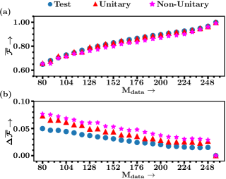
Figure 6: (Color online) (a) Average process fidelity ($\bar{\mathcal{F}}$) and (b) Standard deviation $\Delta\bar{\mathcal{F}}$ obtained for QPT of two-qubit processes using the FFNN model versus size of the dataset ($M_{data}$). For the test dataset (blue dots) the average fidelity is calculated for 3000 processes while for experimental unitary processes (red triangles) and non-unitary processes (magenta stars) the average fidelity is calculated by randomly choosing the reduced dataset $M_{data}$ elements from the full set for four unitary quantum gates and six non-unitary processes, and then repeating the procedure 300 times.

The FFNN results for QPT of various two-qubit experimental quantum processes are shown in Figure 6. The quality of the FFNN is evaluated by means of the average process fidelity $\mathcal{\bar{F}}$, between the process matrix predicted by the FFNN ($\chi_{\rm\small FFNN}$) using a reduced data set of size $M_{data}$ and the process matrix obtained via the standard QPT method ($\chi_{\rm\small STD}$) using a full data set.

Figure 6(a) depicts the performance of the FFNN evaluated on 3000 two-qubit test quantum processes (blue circles), where the $y$-axis denotes the average fidelity $\mathcal{\bar{F}}=\frac{1}{3000}\sum_{n=1}^{3000}\mathcal{\bar{F}}_{n}$, where $\mathcal{\bar{F}}_{n}=\frac{1}{300}\sum_{i=1}^{300}\mathcal{\bar{F}}_{i}$ is the average fidelity of the $n$th test quantum process calculated by randomly constructing an input vector of given size and repeating the process 300 times. Similarly, the red triangles and pink stars correspond to four unitary and six non-unitary quantum processes respectively, obtained from experimental data. The plots given in Figure 6(a) clearly show that the FFNN model is able to predict unitary as well as non-unitary quantum processes from a noisy experimental reduced data set, with good accuracy. For instance, for $M_{{\rm data}}=160$, the FFNN is able to predict the test process with $\mathcal{\bar{F}}=0.8411\pm 0.0284$, whereas the experimental unitary and non-unitary processes are obtained with $\mathcal{\bar{F}}=0.8447\pm 0.038$ and $0.8187\pm 0.0493$, respectively. Hence, the value of $M_{data}$ can be set accordingly, depending on the desired accuracy and precision. The standard deviation in average fidelity $\mathcal{\bar{F}}$ is calculated using Eq. (11) over 3000 quantum processes and is depicted in Figure 6(b). From Figure 6(b), it can be observed that the FFNN model performs better for the QPT of unitary processes as compared to non-unitary processes, since the corresponding process matrices are more sparse.

The experimental fidelity obtained via FFNN of individual quantum processes is given in Figure 8, where the average fidelity is calculated for a set of quantum processes for a given value of the reduced dataset $M_{data}$. For the test dataset the $\mathcal{\bar{F}}$ is calculated over 3000 test processes, whereas for the experimental data set, $\mathcal{\bar{F}}$ is computed over four unitary and six non-unitary processes. For the unitary quantum gates: Identity, CX180, CNOT and CY90, (corresponding to a ‘no operation’ gate, a bit flip gate, a controlled rotation about the $x$-axis by $180^{\circ}$ and a controlled rotation about the $y$-axis by $90^{\circ}$, respectively) the FFNN is able to predict the corresponding process matrix with average fidelities of $\mathcal{\bar{F}}=0.8767\pm 0.0356,0.8216\pm 0.0463,0.8314\pm 0.0387$ and $0.8489\pm 0.0315$ respectively, using a reduced data set of size 160. The six non-unitary processes to be tomographed include free evolution processes for two different times: $D1=0.05$ sec and $D2=0.5$ sec, a magnetic field gradient pulse (MFGP), and three error channels, namely, a correlated bit flip (CBF) channel, a correlated phase flip (CPF) channel, and a correlated bit-phase flip (CBPF) channel. There are several noise channels acting simultaneously all the qubits, during the free evolution times $D1$ and $D2$, such as the phase damping channel (corresponding to the T₂ NMR relaxation process) and the amplitude damping channel (corresponding to the T₁ NMR relaxation process). The MFGP process is typically implemented using gradient coils in NMR hardware where the magnetic field gradient is along the $z$-axis. The MFGP process to be tomographed is a sine-shaped pulse of duration of 1000$\mu$s, 100 time intervals = 100 and an applied gradient strength of 15%. For the intrinsic non-unitary quantum processes D1 D2, and the MFGP, the FFNN is able to predict the corresponding process matrix with average fidelities of $\mathcal{\bar{F}}=0.8373\pm 0.0381,0.7607\pm 0.0690$ and $0.7858\pm 0.0703$ respectively, using a reduced data set of size 160. It is evident from the computed fidelity values that the FFNN performs better if the process matrix is sparse.

Table 4: Experimental fidelities $\mathcal{F}$ computed between $\chi_{\small{\rm FFNN}}$, the process matrix predicted via FFNN using a full data set, and $\chi_{\small{\rm STD}}$, the process matrix obtained via the standard QPT method.

Unitary Process	$\mathcal{F}$	Non-Unitary Process	$\mathcal{F}$
Test	0.9997	D1	0.9987
Identity	0.9943	D2	0.9635
CNOT	0.9996	Grad	0.9917
CX180	0.9996	CBF	0.9943
CY90	0.9996	CPF	0.9996
		CBPF	0.9996

Although our main goal is to prove that the FFNN is able to reconstruct quantum states and processes with a high fidelity even for heavily reduced datasets, we also wanted to verify the efficacy of the network when applied to a complete data set. The values of process fidelity obtained via FFNN for the full data set are shown in Table 4, where it is clearly evident that the FFNN is able to predict the underlying quantum process with very high fidelity, and works accurately even for non-unitary quantum processes. The somewhat lower fidelity of the D2 process as compared to other quantum processes can be attributed to the corresponding process matrix being less sparse.

IV.2 FFNN Reconstruction of Correlated Noise Channels

The duality simulation algorithm (DSA) can be used to simulate fully correlated two-qubit noise channels, namely the CBF, CPF and CBPF channels Xin et al. (2017). The FFNN model is then employed to fully characterize these channels. DSA allows us to simulate the arbitrary dynamics of an open quantum system in a single experiment where the ancilla system has a dimension equal to the total number of Kraus operators characterizing the given quantum channel. An arbitrary quantum channel having $d$ Kraus operators can be simulated via DSA using unitary operations $V$, $W$, and the control operation $U_{c}=\sum_{i=0}^{d-1}|i\rangle\langle i|\otimes U_{i}$ such that the following condition is satisfied:

$$E_{k}=\sum_{i=0}^{d-1}W_{ki}V_{i0}U_{i}\quad(k=0,1,2,...,d-1)$$ (12)

where $E_{k}$ is the Kraus operator, and $V_{i0}$ and $W_{ki}$ are the elements of $V$ and $W$, respectively. The quantum circuit for DSA is given in Reference Xin et al. (2017), where the initial state of the system is encoded as $|0\rangle_{a}\otimes|\psi\rangle_{s}$ which is then acted upon by $V\otimes I$ followed by $U_{c}$ and $W\otimes I$, and finally a measurement is performed on the system qubits.

For this study, the two-qubit CBF, CPF and CBPF channels are characterized using two Kraus operators as:

CBF $$:E_{0}=\sqrt{1-p}I^{\otimes 2},\quad E_{1}=\sqrt{p}\sigma_{x}^{\otimes 2}$$

CPF $$:E_{0}=\sqrt{1-p}I^{\otimes 2},\quad E_{1}=\sqrt{p}\sigma_{z}^{\otimes 2}$$

CBPF $$:E_{0}=\sqrt{1-p}I^{\otimes 2},\quad E_{1}=\sqrt{p}\sigma_{y}^{\otimes 2}$$ (13)

where $p$ is the noise strength, which can also be interpreted as probability with which the state of the system is affected by the given noise channel. For $p=0$ the state of the system is unaffected, and for $p=1$ the state of the system is maximally affected by the given noise channel. Since all the three noise channels considered in this study have only two Kraus operators, they can be simulated using a single ancilla qubit. Hence for all three noise channels, one can set $V=\left(\begin{array}[]{cc}\sqrt{1-p}&-\sqrt{p}\\ \sqrt{p}&\sqrt{1-p}\end{array}\right)$, $W=I$, and $U_{0}=I\otimes I$. The different $U_{1}$ for CBF, CPF and CBPF channels are set to $\sigma_{x}\otimes\sigma_{x}$, $\sigma_{z}\otimes\sigma_{z}$ and $\sigma_{y}\otimes\sigma_{y}$ respectively, such that the condition given in Eq. (12) is satisfied. Note that $V$ can be interpreted as a rotation about the $y$-axis by an angle $\theta$ such that $p=\sin^{2}{(\frac{\theta}{2})}$.

The generalized quantum circuit using DSA to simulate all three error channels is given in Figure 7. For the CBF channel, $U_{c}$ turns out to be a Control-NOT-NOT gate, where the value of $\theta$ (Figure 7) is zero. For the CPF and the CBPF channels, the values of $\theta,\phi$ (the angle and axis of rotation) are $(\frac{\pi}{2},y)$ and ($\frac{\pi}{2},z$), respectively. The output from the tomographic measurements on the system qubits forms the column vector $\overrightarrow{\lambda}$. For a given value of $p$, the full vector $\overrightarrow{\lambda}$ can be constructed by preparing the system qubits in a complete set of linearly independent input states.

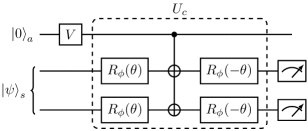
Figure 7: Quantum circuit to simulate the action of a correlated bit flip, a correlated phase flip and a correlated bit+phase flip noise channel. $|\psi\rangle_{s}$ are a set of linearly independent two-qubit input states, $|0\rangle_{a}$ denotes the state of the ancilla, $V$ is a single-qubit rotation gate and $U_{c}$ denotes a set of control operations with varying values of $(\theta,\phi)$, depending on the noise channel being simulated.

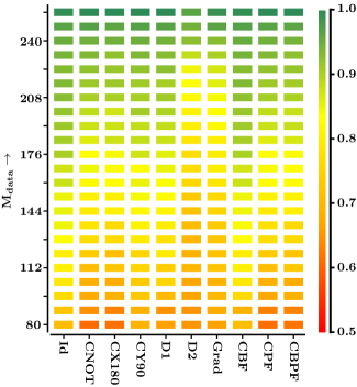
Figure 8: (Color online) Process fidelity ($\bar{\mathcal{F}}$) between FFNN model and the standard linear inversion method vs size of the heavily reduced dataset ($M_{data}$), for different unitary and non-unitary quantum processes. The various quantum processes are labeled on the $x$-axis and the color coded bar on the right represents the value of the fidelity.

As can be seen from Figure 8, the average fidelity $\mathcal{\bar{F}}=0.8738\pm 0.0366,0.8272\pm 0.0403$ and $0.8273\pm 0.0416$ for the experimentally simulated noise channels CBF, CPF and CBPF respectively, using a reduced data set of size 160. Since all three correlated noise channels are characterized by only two Kraus operators, the corresponding process matrices turn out to be sufficiently sparse (with only two non-zero elements in the process matrix). The FFNN can hence be used to accurately tomograph such noise channels with arbitrary noise strength using a heavily reduced dataset.

V Conclusions

Much recent research has focused on training artificial neural networks to perform several quantum information processing tasks including tomography, entanglement characterization and quantum gate optimization. We designed and applied a FFNN to perform QST and QPT on experimental NMR data, in order to reconstruct the density and process matrices which characterize the true quantum state and process, respectively. The FFNN is able to predict the true quantum state and process with very high fidelity and performs in an exemplary fashion even when the experimental data set is heavily reduced. Compressed sensing is another method which also uses reduced data sets to perform tomography of quantum states and processes. However, this method requires prior knowledge such as system noise and also requires that the basis in which the desired state (process) is to be tomographed should be sufficiently sparse. The FFNN, on the other hand, does not need any such prior knowledge and works well for all types of quantum states and processes. Moreover, working with a heavily reduced data set has the benefit of substantially reducing experimental complexity since performing tomographically complete experiments grows exponentially with system size. One can perform very few experiments and feed this minimal experimental dataset as inputs to the FFNN, which can then reconstruct the true density or process matrix. Our results hence demonstrate that FFNN architectures are promising methods for performing QST and QPT of large qubit registers and are an attractive alternative to standard methods, since they require substantially fewer resources.