List-Based Detection and Selection of Access Points in Cell-Free Massive MIMO Networks

Abstract

This paper proposes a cell-free massive multiple- input multiple-output (CF-mMIMO) architecture with joint list- based detection with soft interference cancelation (soft-IC) and access points (APs) selection. In particular, we derive a new closed-form expression for the minimum mean-square error receive filter while taking the uplink transmit powers and APs selection into account. This is achieved by optimizing the receive combining vector by minimizing the mean square error between the detected symbol estimate and transmitted symbol, after canceling the multi-user interference (MUI). By using low-density parity check (LDPC) codes, an iterative detection and decoding (IDD) scheme based on a message passing is devised. In order to perform joint detection at the central processing unit (CPU), the access points locally estimate the channel and send their received sample data to the CPU via the front haul links. In order to enhance the system’s bit error rate performance, the detected symbols are iteratively exchanged between the joint detector and the LDPC decoder in log likelihood ratio form. Furthermore, we draw insights into the derived detector as the number of IDD iterations increase. Finally, the proposed list detector is compared with existing detection techniques.

I Introduction

Unlike centralized massive multiple-input multiple-output (MIMO) systems [1, 2], cell-free massive MIMO (CF-mMIMO) systems operate by deploying a relatively large number of either single-antenna or multiple-antenna access points (APs) in a distributed fashion. The aim is to increase the network throughput, coverage, spectral efficiency, energy efficiency and quality of service [3]. The APs send their received data signals to a central processing unit (CPU) for information processing and detection. The CPU operates the system at a network level with the aim of coherent transmission and reception without necessarily requiring cell boundaries [4]. Earlier works on CF-mMIMO considered system architectures where the UEs are equipped with single antennas and served by multiple APs [4]. However, such systems require a significant number of front haul links between the APs and the CPU. More recent developments in the CF-mMIMO architecture have considered APs selection strategies that are capable of reducing the complexity in the system architecture as well as yielding more practical implementations. These APs selection methods are capable of achieving close to the entire network performance but with an added advantage of reducing the signaling overheads [3, 5, 6]. CF-mMIMO networks are liable to multi-user interference (MUI) caused by pilot contamination as well as the overlapping of the signals transmitted by the users during uplink data transmission phase [7]. MUI makes the receiver design complex and thus calls for efficient techniques in the design of CF-mMIMO receivers. The key aspect in the design of efficient receivers lies at reducing the error between detected symbol and transmitted symbol data [10, 14, 15, 16].

The performance of CF-mMIMO receivers can be enhanced by error correcting codes (ECC) such as low-density parity check (LDPC) [8, 9] and turbo codes [10]. The use of iterative detection and decoding (IDD) techniques has been extensively studied to improve the performance of co-located MIMO (Col-MIMO) and massive MIMO (mMIMO) [10, 14, 15, 16]. IDD-based detection techniques leverage on message passing by exchanging soft beliefs in terms of log-likelihood ratios (LLRs) between the detector and the decoder. LDPC codes are cost-effective and have been used in the state-of-the art standards to improve the performance of MIMO systems [16, 22, 12, 13].

In this work, we present a joint IDD scheme with APs selection assuming imperfect channel estimation and taking the UL transmission powers and joint detection at the CPU into account. Particularly, we derive a new closed-form expression for the MMSE detector with soft interference cancellation (MMSE-soft-IC). Based on the available a-priori information about the expectation of the transmitted symbol estimate, we draw insights into the derived detector and present the MMSE filters for the uplink as the number of IDD iterations increase. Furthermore, we propose a list-based detector to reduce the error propagation that exists in the interference cancellation step. The bit error (BER) performance of the proposed list-based detector and APs selection is compared with soft MMSE and MMSE-soft-IC detection techniques, for the system with APs selection (APs-Sel) and without APs selection (All-APs).

The rest of this paper is organized as follows: Section II presents the proposed centralized system model for the CF-mMIMO architecture, the channel estimation and APs selection criterion. The derived receive filter analysis and insights are presented in section III. The proposed list-based detector is presented in IV. Section V discusses the IDD scheme. Simulation results and discussions are presented in VI. Section VII gives the concluding remarks.

Symbol notations: Lower bold and upper bold letters are used to represent vectors and matrices, respectively. The Hermitian transpose operator is denoted by $(\cdot)^{H}$, $\mathbb{E}\left\{x\right\}$ denotes the expected value of random variable $X$.

II Proposed System Model

We consider an uplink CF-mMIMO system model with imperfect channel estimation. More specifically, an LDPC-coded CF-mMIMO system comprising of $L$ APs each equipped with $N$ receive antennas, $K$ single-antenna user equipment (UEs), a joint detector and an LDPC decoder at the CPU for the considered centralized processing scenario is considered as shown in Figure 1.

Figure 1: Block diagram for IDD scheme with Centralized Processing.

The data are first encoded (Enc) by an LDPC encoder having a code rate ${R}$. This encoded sequence is then modulated (Mod) to complex symbols with a complex constellation of $2^{M_{c}}$ possible signal points and average energy $E_{s}$. The coded data is then transmitted by ${K}$ UEs to the APs. During the data reception, the APs act as relays and send the received information to the CPU which comprises of a joint detector and an LDPC decoder. Then the joint detector sends the received soft information $\Lambda_{E}$ in the form of LLRs to the LDPC decoder. The decoder adopts an iterative strategy by sending extrinsic information $\Lambda_{U}$ to the joint detector which improves the performance of the entire network. Additionally, the performance of the proposed detector is examined for the case with and without iterations.

II-A Uplink Pilot Transmission and Channel Estimation

We start by assuming $\tau_{p}-$length pilot mutually orthogonal signals $\psi_{1}$, …, $\psi_{\tau_{p}}$ with $\psi_{t}\psi^{*}_{t}=1$ are used to estimate the channel. Furthermore, we assume that $K>\tau_{p}$ such that more than one UE can be assigned per pilot. The index of UE $k$ that uses the same pilot is denoted as $t_{k}\in\left\{1,...,\tau_{p}\right\}$ with $\vartheta_{k}\subset\left\{1,...,K\right\}$ as the subset of UEs that use the same pilot as UE $k$ inclusive. The received $\mathbf{R}_{l}$ complex $N\times\tau_{p}$ signal after the UE transmission [3] is given by

$$\mathbf{R}_{l}=\sum_{j=1}^{K}\sqrt{\eta_{j}}\mathbf{g}_{jl}\bm{\psi}^{T}_{t_{j}}+\mathbf{N}_{l},$$ (1)

where $\eta_{j}$ is the transmit power from UE $j$, $\mathbf{N}_{l}$ is a receiver noise signal with independent ${\mathcal{N}}_{\mathbb{C}}\sim\left(0,\sigma^{2}\right)$ with noise power $\sigma^{2}$, $\mathbf{g}_{jl}\sim\mathcal{N}_{\mathbb{C}}\left(0,\bm{\Omega}_{jl}\right)$, and $\bm{\Omega}_{jl}\in\mathbb{C}^{NL\times NL}$ is the spatial correlation matrix that describes the channel’s spatial properties between the $k$-th UE and $l$-th AP, $\beta_{k,l}\triangleq\frac{\mathrm{tr}\left(\bm{\Omega}_{jl}\right)}{N}$ is the large-scale (LS) fading coefficient. The AP first correlates the received signal with the associated normalized pilot signal $\bm{\psi}_{t_{k}}/\sqrt{\tau_{p}}$ to $\mathbf{r}_{t_{kl}}\triangleq\frac{1}{\sqrt{\tau_{p}}}\mathbf{R}_{l}\bm{\psi}^{*}_{t_{k}}\in\mathbb{C}^{N}$ to estimate the channel $\mathbf{g}_{jl}$ given by

$$\mathbf{r}_{t_{kl}}=\sum_{j\in\vartheta_{k}}\sqrt{\eta_{j}\tau_{p}}\mathbf{g}_{jl}+\mathbf{n}_{t_{kl}},$$ (2)

where $\mathbf{n}_{t_{kl}}\triangleq\frac{1}{\sqrt{\tau_{p}}}\mathbf{N}_{l}\bm{\psi}^{*}_{t_{k}}\sim\mathcal{N}_{c}\left(0,\sigma^{2}\mathbf{I}_{N}\right)$ is the obtained noise sample after estimation. Using [3], the MMSE estimate of $\mathbf{g}_{kl}$ is given by

$$\hat{\mathbf{g}}_{kl}=\sqrt{\eta_{k}\tau_{p}}\bm{\Omega}_{kl}\Psi^{-1}_{t_{k}}\mathbf{r}_{t_{kl}},$$ (3)

where $\Psi_{t_{kl}}=\mathbb{E}\left\{\mathbf{r}_{t_{kl}}\mathbf{r}^{H}_{t_{kl}}\right\}=\sum_{j\in\vartheta_{k}}{\eta_{j}\tau_{p}}\mathbf{\Omega}_{jl}+\mathbf{I}_{N}$ is the received signal vector correlation matrix. The channel estimate $\hat{\mathbf{g}}_{kl}$ and estimation error $\tilde{\mathbf{g}}_{kl}=\mathbf{g}_{kl}-\hat{\mathbf{g}}_{kl}$ are independent with distributions $\hat{\mathbf{g}}_{kl}\sim\mathcal{N}_{c}\left(0,\eta_{k}\tau_{p}\bm{\Omega}_{kl}\mathbf{\Psi}^{-1}\bm{\Omega}_{kl}\right)$ and $\tilde{\mathbf{g}}_{kl}\sim\mathcal{N}_{c}\left(0,\mathbf{C}_{kl}\right)$, where the parameter $\mathbf{C}_{kl}$ is given by

$$\mathbf{C}_{kl}=\mathbb{E}\left\{\tilde{\mathbf{g}}_{kl}\tilde{\mathbf{g}}^{H}_{kl}\right\}=\bm{\Omega}_{kl}-\eta_{k}\tau_{p}\bm{\Omega}_{kl}\mathbf{\Psi}^{-1}\bm{\Omega}_{kl}.$$ (4)

Pilot-contamination is created by the mutual interference generated by the UEs sharing the same pilot signals. This degrades the system’s performance [3]. The received signal vector at the APs is given by

$$\mathbf{y}=\sum_{j=1}^{K}\mathbf{g}_{j}s_{j}+\mathbf{n}.$$ (5)

This can be given in a more compact representation as

$$\mathbf{y}=\mathbf{G}\mathbf{s}+\mathbf{n},$$ (6)

where ${\mathbf{G}}$ $\in\mathbb{C}^{NL\times K}$ is the channel matrix with both small scale and LS fading coefficients. $\mathbf{s}=[s_{1},..,s_{k-1},s_{k},s_{k+1},...,s_{K}]$ denotes the transmit symbol vector with $\mathbb{E}\left\{s_{k}s^{*}_{k}\right\}=\rho_{k}$, $\bm{\rho}=\left[\rho_{1},..,\rho_{K}\right]^{T}$ is the average transmit power vector, $\mathbf{n}$ is the additive white Gaussian noise sample (AWGN) with zero mean and unit variance.

II-B Access Point Selection Procedure

The APs selection considers an improved dynamic cooperation clustering (DCC) approach presented in [3]. This is achieved by forming a block diagonal matrix $\mathbf{D}_{kl}=\mathrm{diag}\left(\mathbf{D}_{k1},..,\mathbf{D}_{kL}\right)\in\mathbb{C}^{NL\times NL}$, where $k=1,..,K$ and $l=1,..,L$. The matrix determines which APs antennas or AP for the case of single-antenna APs is going to serve a particular UE. Then the set of UEs served by AP $l$ is given by

$$\mathcal{D}_{l}=\biggl{\{}k:\mathrm{tr}\left(\mathbf{D}_{kl}\right)\geq 1,k\in\left\{1,..,K\right\}\biggr{\}}.$$ (7)

. The DCC does not alter the received signal because all APs physically receive the broadcast signal. The key aspect is to only have a set of selected APs to take part during signal detection. The the received signal after AP selection is given by

$$\mathbf{y}=\mathbf{D}_{k}\mathbf{G}\mathbf{s}+\mathbf{D}_{k}\mathbf{n},$$ (8)

where $\mathbf{D}_{k}=\mathrm{diag}\left(\mathbf{D}_{k1},..,\mathbf{D}_{kL}\right)$ is a block diagonal matrix which determines which APs are serving a given UE or set of UEs. A special case occurs when $\mathbf{D_{k}}=\mathbf{I}_{NL}$. This implies that all the UEs are served by all APs, implying that (8) reduces to (6). The choice of which AP(s) participate in service of particular UE is based on the joint access point selection algorithm presented in [3]. In this case the UE appoints a master AP that is used to coordinate UL detection and decoding based on the largest large scale fading (LLSF) coefficient. The CPU then sets threshold a value $\beta_{th}$ for other non-master APs to participate in services of a particular UE. Further details of this selection algorithm can be found in [3].

III Proposed Receiver Design

In this section, we present the derivations of the proposed receive filter and structure. The proposed detector is capable of canceling the MUI that occurs due to the other $K-1$ UEs in the network. Thus, we propose a detector that comprises an MMSE filter followed by a soft interference canceler. The demodulator forms soft estimates of the transmitted symbols by computing the symbol mean $\bar{s}_{j}$ based on the available soft beliefs or a-priori information from the LDPC decoder [14]. This symbol mean is key in the cancellation step because it determines if we have a perfect interference canceler or a conventional MMSE filter as the number of iterations increase. The symbol mean $\mathbb{E}\left\{s_{j}\right\}=\bar{s_{j}}$ is given by

$$\bar{s}_{j}=\sum_{s\in{A}}sP(s_{j}=s),$$ (9)

where ${A}$ is the complex constellation set. The variance of the $j$-th user symbol is computed as

$$\sigma^{2}_{j}=\sum_{s\in\mathcal{A}}|s-\bar{s}_{j}|^{2}P(s_{j}=s).$$ (10)

The a-priori probabilities obtained from the extrinsic LLRs are given by

$$P(s_{j}=s)=\prod_{l=1}^{M_{c}}[1+\exp(-s^{b_{l}}\Lambda_{c}(b_{(j-1)M_{c}+l}))]^{-1},$$ (11)

where $s^{b_{l}}\in(+1,-1)$ denotes the value of the $l$-th bit of symbol $s$, $\Lambda_{c}(b_{i})$ denotes the extrinsic LLR of the $i$-th bit computed by the LDPC decoder in the previous iteration. We define $\Lambda_{c}(b_{i})=0$ at the first iteration since the only available belief is from the channel. The probabilities in (11) are obtained by assuming statistical independence of bits within the same symbol [14]. Next we present the derivations of the proposed MMSE-soft-IC detector.

Centralized Processing With APs Selection: The aim of the centralized detection after APs selection is to avoid redundant processing of poor quality signals. Also the number of front haul links significantly reduce which makes the system more scalable [3]. This leads to a more efficient implementation of the CF-mMIMO system as well as avoiding wastage of resources. The major draw back of such a selection scheme is the slight reduction in performance. Therefore, there is a trade off between performance and hardware complexity in the design by using AP selection techniques. The received signal after APs selection is given by

$$\mathbf{y}^{CP}=$$ (12)

$$\mathbf{D}_{k}\hat{\mathbf{g}}_{k}s_{k}+\mathbf{D}_{k}\hat{\mathbf{G}}_{\text{i}}\mathbf{s}_{\text{i}}+\sum_{m=1}^{K}\mathbf{D}_{k}\tilde{\mathbf{g}}_{m}s_{m}+\mathbf{D}_{k}\mathbf{n},$$

where $\mathbf{y}^{CP}$ is an $NL\times 1$ vector consisting of the received signals after APs selection, The parameters $s_{k}$, $\hat{\mathbf{g}}_{k}$, are the transmitted symbol, $NL\times 1$ estimated channel vector for the $k-$th UE, respectively. The parameters $\mathbf{s}_{\text{i}}$, $\hat{\mathbf{G}}_{\text{i}}$ denote the $K-1\times 1$ transmitted symbol vector and the $NL\times K-1$ estimated channel matrix for the other $K-1$ UEs, respectively. The parameter $s_{m}$ and $\tilde{\mathbf{g}}_{m}$ are the transmitted symbol vector during channel estimation and channel estimation error vector, respectively.

The decision statistic $y_{k}$ of the $k$-th user stream after applying the receive combining vector $\mathbf{w}_{k}$ is given by

$$y^{CP}_{k}=$$ (13)

$$\mathbf{w}^{H}_{k}\biggl{(}\underbrace{\mathbf{D}_{k}\hat{\mathbf{g}}_{k}s_{k}}_{{\beta}_{k}}+\underbrace{\mathbf{D}_{k}\hat{\mathbf{G}}_{\text{i}}\mathbf{s}_{\text{i}}}_{\lambda_{\text{i}}}+\underbrace{\sum_{m=1}^{K}\mathbf{D}_{k}\tilde{\mathbf{g}}_{m}s_{m}}_{\alpha_{\text{e}}}+\underbrace{\mathbf{D}_{k}\mathbf{n}}_{\gamma_{n}}\biggr{)},$$

where $\mathbf{\beta}_{k}$, ${\lambda_{\text{i}}}$, $\alpha_{\text{e}}$, $\gamma_{k}$ denote the desired signal for $k$-th UE, the MUI from the other $K-1$ UEs, the channel estimation error term and the phase-rotated noise. The estimated detected symbol at the CPU after removing the MUI is given by

$$\tilde{s}_{k}=\mathbf{w}^{H}_{k}\mathbf{y}^{CP}-\mathbf{w}^{H}_{k}\mathbf{D}_{k}\hat{\mathbf{G}}_{\text{i}}\bar{\mathbf{s}}_{\text{i}}.$$ (14)

The optimization of the receive combining vector $\mathbf{w}_{k}$ enables us to minimize the mean square error in the detected data-stream. We follow similar procedures in [10, 11] by optimizing the linear detection vector $\mathbf{w}_{k}$. The optimization problem is formulated as:

$$\mathbf{w}_{k}=\mathsf{arg}\min_{\left(\mathbf{w}_{k}\right)}\mathbb{E}\biggl{\{}||\tilde{s}_{k}-s_{k}||^{2}\mid\hat{\mathbf{G}}\biggr{\}}.$$ (15)

The term $\mathbb{E}\left\{||\tilde{s}_{k}-s_{k}||^{2}\mid\hat{\mathbf{G}}\right\}$ in (15) is given on the top of the next page by (III).

 

$$\mathbb{E}\biggl{\{}||\tilde{s}_{k}-s_{k}||^{2}\mid\hat{\mathbf{G}}\biggr{\}}= \mathbf{w}^{H}_{k}\biggl{(}\mathbf{D}_{k}\biggl{(}\rho_{k}\hat{\mathbf{g}}_{k}\hat{\mathbf{g}}^{H}_{k}+\hat{\mathbf{G}}_{\text{i}}\mathbf{\Delta}_{\text{i}}\hat{\mathbf{G}}^{H}_{\text{i}}\biggr{)}\mathbf{D}^{H}_{k}+\mathbf{D}_{k}\biggl{(}\sum_{m=1}^{K}\left(\mid\bar{s}_{m}\mid^{2}+\sigma^{2}_{m}\right)\mathbf{C}_{m}+\sigma^{2}\mathbf{{I}}_{NL}\biggr{)}\mathbf{D}^{H}_{k}\biggr{)}\mathbf{w}_{k}$$

$$-\rho_{k}\mathbf{w}^{H}_{k}\mathbf{D}_{k}\hat{\mathbf{g}}_{k}-\rho^{*}_{k}\hat{\mathbf{g}}^{H}_{k}\mathbf{D}^{H}_{k}\mathbf{w}_{k}+\rho_{k}.$$ (16)

 

Where $\mathbf{C}_{m}$ is the cross-correlation matrix from channel estimation error of the $m$-th UE, the matrix $\mathbf{\Delta}_{i}=\mathsf{diag}\left[{\sigma_{{1}}^{2}},...,{\sigma_{{k-1}}^{2}},{\sigma_{{k+1}}^{2}},...,{\sigma_{{K}}^{2}}\right]$ in (III) is highly relevant in the IDD scheme during the soft-IC step. Differentiating (III) with respect to (w.r.t) $\mathbf{w}^{*}_{k}$ and equating to zero yields

$$\mathbf{w}^{\mathrm{APS-Sel}}_{k}=\rho_{k}\biggl{(}\mathbf{D}_{k}\biggl{(}\rho_{k}\hat{\mathbf{g}}_{k}\hat{\mathbf{g}}^{H}_{k}+\hat{\mathbf{G}}_{\text{i}}\mathbf{\Delta}_{\text{i}}\hat{\mathbf{G}}^{H}_{\text{i}}\biggr{)}\mathbf{D}^{H}_{k}$$

$$+\mathbf{D}_{k}\biggl{(}\sigma^{2}\mathbf{{I}}_{NL}+\sum_{m=1}^{K}\left(\mid\bar{s}_{m}\mid^{2}+\sigma^{2}_{m}\right)\mathbf{C}_{m}\biggr{)}\mathbf{D}^{H}_{k}\biggr{)}^{-1}$$

$$\times\mathbf{D}_{k}\hat{\mathbf{g}}_{k},$$ (17)

III-1 Insights into the obtained detector

The MMSE- soft-IC detector for the scenario that uses all APs can be obtain from (III) by taking a special case when $\mathbf{D}_{k}=\mathbf{I}_{NL}$, and is given by

$$\mathbf{w}^{\mathrm{All-APs}}_{k}=\rho_{k}\biggl{(}\rho_{k}\hat{\mathbf{g}}_{k}\hat{\mathbf{g}}^{H}_{k}+\hat{\mathbf{G}}_{\text{i}}\bm{\Delta}_{\text{i}}\hat{\mathbf{G}}^{H}_{\text{i}}$$

$$+\sigma^{2}\mathbf{{I}}_{NL}+\sum_{m=1}^{K}\left(\mid\bar{s}_{m}\mid^{2}+\sigma^{2}_{m}\right)\mathbf{C}_{m}\biggr{)}^{-1}\hat{\mathbf{g}}_{k}.$$ (18)

For the first iteration, $\bar{\mathbf{s}}_{\text{i}}=\mathbf{0}$ in (9). In this case we have a linear MMSE filter and the detected signal in (14) is given by

$$\tilde{s}_{k}=\rho_{k}\hat{\mathbf{g}}^{H}_{k}\mathbf{D}^{H}_{k}\biggl{(}\rho_{k}\mathbf{D}_{k}\hat{\mathbf{g}}_{k}\hat{\mathbf{g}}^{H}_{k}\mathbf{D}^{H}_{k}+\mathbf{D}_{k}\hat{\mathbf{G}}_{\text{i}}~{}\mathrm{diag}\left(\bm{\rho}_{\text{i}}\right)\hat{\mathbf{G}}^{H}_{\text{i}}\mathbf{D}^{H}_{k}$$

$$+\mathbf{D}_{k}\left(\sigma^{2}\mathbf{I}_{NL}+\sum_{m=1}^{K}\rho_{m}\mathbf{C}_{m}\right)\mathbf{D}^{H}_{k}\biggr{)}^{-1}\mathbf{y}^{CP},$$ (19)

where $\bm{\rho}_{i}$ denotes the average transmit power vector for the other $K-1$ UEs. As the number of iterations increases, $\bar{\mathbf{s}}_{\text{i}}\approx\mathbf{s}_{\text{i}}$ in (9). In such a scenario, the filter becomes a perfect interference canceler and thus (14) yields

$$\tilde{s}_{k}=\rho_{k}\hat{\mathbf{g}}^{H}_{k}\mathbf{D}^{H}_{k}\biggl{(}\rho_{k}\mathbf{D}_{k}\hat{\mathbf{g}}_{k}\hat{\mathbf{g}}^{H}_{k}\mathbf{D}^{H}_{k}+\mathbf{D}_{k}\biggl{(}\sigma^{2}\mathbf{I}_{NL}$$

$$+\sum_{m=1}^{K}\mid s_{m}\mid^{2}\mathbf{C}_{m}\biggr{)}\mathbf{D}^{H}_{k}\biggr{)}^{-1}\left(\mathbf{y}^{CP}-\mathbf{D}_{k}\hat{\mathbf{G}}_{\text{i}}\mathbf{s}_{\text{i}}\right).$$ (20)

IV List-based detector

In this section, we describe the operation of the proposed list-based detection scheme shown in Fig.2, which has been inspired by the works in [15, 16, 17, 18, 20].

Figure 2: Block diagram of the proposed list-based detector.

The design takes advantage of list feedback (LF) diversity by selecting a list of constellation candidates if there is unreliability of the previously detected symbols [16]. In this case, a shadow area constraint (SAC) is initiated in order to obtain an optimal feedback candidate. The SAC is capable of reducing search space from growing exponentially as well as reducing the computational complexity. The key idea of such a selection criterion is to avoid redundant processing when there is a reliable decision. The procedure of obtaining the detected symbol $\hat{s}_{k}$ of the $k$-th user is analogous to the steps presented in [16]. The $k$-th user soft estimate is obtained by $u_{k}=\mathbf{w}_{k}^{H}\check{\mathbf{y}}_{k}$. The filter $\mathbf{w}_{k}$ is similar to the receive MMSE filter in (III-1) and $\check{\mathbf{y}}_{k}=\mathbf{y}^{CP}-\sum_{t=1}^{k-1}\mathbf{D}_{k}\hat{\mathbf{g}}_{t}\hat{{s}}_{t}$ represents the received vector following the soft cancellation of the $k-1$ symbols that were previously detected. The SAC assesses the reliability of this decision using the soft estimate $u_{k}$ for each layer according to

$$d_{k}=|u_{k}-\nu_{f}|,$$ (21)

where $\nu_{f}=\mathsf{arg}\min_{\mathbf{\nu_{f}}\in{\mathcal{A}}}\left\{|u_{k}-\nu_{f}|\right\}$ denotes the closest constellation point to the $k$-th user soft estimate $u_{k}$. If $d_{k}>d_{\text{th}}$ the chosen constellation point gets dumped into the shadow area of the constellation map since the choice is deemed to be unreliable. Parameter $d_{\text{th}}$ is the predefined threshold euclidean distance to guarantee reliability of the selected symbol [16]. The list-based algorithm performs a hard slice for UE $k$ as in the soft-IC if there is reliability of the soft estimate $u_{k}$. In this case, $\hat{s}_{k}=Q(u_{k})$ is the estimated symbol, where $Q(\cdot)$ is the quantization notation which maps to the constellation symbol closest to $u_{k}$.

Otherwise, the decision is deemed unreliable. In this case, a list of candidates $\mathcal{L}=\{c_{1},c_{2},...,c_{m},...,c_{M}\}\subseteq\mathcal{A}$ is generated, which is made up of the constellation $M$ points that are closest to $u_{k}$. The number of candidate points $M$ is given by the QPSK symbols. The algorithm selects an optimal candidate $c_{m,\text{opt}}$ from a list of $\mathcal{L}$ candidates. Thus, the unreliable choice $Q(u_{k})$ is replaced by a hard decision and $\hat{s}_{k}=c_{m,\text{opt}}$ is obtained. The list-based detector first defines the selection vectors $\bm{\phi}^{1},\bm{\phi}^{2},...,\bm{\phi}^{m},...\bm{\phi}^{M}$ whose size is equal to the number of the constellation candidates that are used every time a decision is considered unreliable. For example, for the $k$-th layer, a $K\times 1$ vector $\bm{\phi}^{m}=\left[\hat{s}_{1},...,\hat{s}_{k-1},c_{m},\phi^{m}_{k+1},...,\phi^{m}_{q},...,\phi^{m}_{K}\right]^{T}$ which is a potential choice corresponding to $c_{m}$ in the k-th user comprise the following items: (a) The previously estimated symbols $\hat{s}_{1},\hat{s}_{2},...,\hat{s}_{k-1}$. (b) The candidate symbol $c_{m}$ obtained from the constellation for subtracting a decision that was considered unreliable $Q(u_{k})$ of the k-th user. (c) Using (a) and (b) as the previous decisions, detection of the next user data $k+1,...,q,...,$ $K$-th is performed by the soft-IC approach. Mathematically, the choice $\phi^{m}$ is given by [16]

$$\phi^{m}_{q}=Q(\mathbf{w}^{H}_{q}{\hat{\bm{y}}}^{m}_{q}),$$ (22)

where the index $q$ denotes a given UE between the $k+1$-th and the $K$-th UE, $\hat{\bm{y}}^{m}_{q}=\check{\bm{y}}_{k}-\mathbf{D}_{k}\hat{\mathbf{g}}_{k}c_{m}-\mathbf{D}_{k}\sum_{p=k+1}^{q-1}\hat{\mathbf{g}}_{p}\phi^{m}_{p}$. A key attribute of the list-based detector is that the same MMSE filter $\mathbf{w}_{k}$ is used for all the constellation candidates. Therefore, it has the same computational cost as the conventional soft-IC. The optimal candidate ${m,\text{opt}}$ is selected according to the local maximum likelihood (ML) rule given by

$${m,\text{opt}}=\mathsf{arg}\min_{1\leq m\leq M}\left\|\bm{y}^{CP}-\mathbf{D}_{k}\hat{\mathbf{G}}\bm{\phi}^{m}\right\|^{2}.$$ (23)

V Iterative detection and decoding

In this section, the MMSE- based detectors are presented for the IDD scheme as shown in Fig. 1, consisting of a joint detector and an LDPC decoder. The received signal at the output of the filter, contains the desired symbol, MUI, the channel estimation error and noise. We use similar assumptions given in [10, 14, 13] to approximate the parameter $u_{k}$ as an AWGN channel given by

$$u_{k}=\omega_{k}s_{k}+z_{k},$$ (24)

where the parameter $\omega_{k}$ is given by $\mathbb{E}\{{s}^{*}_{k}u_{k}\}=\rho_{k}\mathbf{w}^{H}_{k}\mathbf{D}_{k}\hat{\mathbf{g}}_{k}$. The parameter $z_{k}$ is a zero-mean AWGN variable. Using similar procedures as in [16], variance of $z_{k}$ is given by $\kappa^{2}_{k}=\mathbb{E}\left\{\mid u_{k}-\omega_{k}s_{k}\mid^{2}\right\}=\mathbf{w}^{H}_{k}\mathbf{D}_{k}\left(\sum_{m=1}^{K}\rho_{m}\mathbf{C}_{m}+\sigma^{2}\mathbf{I}_{NL}\right)\mathbf{D}^{H}_{k}\mathbf{w}_{k}$. The extrinsic LLR computed by the detector for the $l$-th bit $l\in\left\{1,2,...,M_{c}\right\}$ of the symbol $s_{k}$ transmitted by the $k$-th user is [10, 14]

$$\Lambda_{E}\left(b_{(k-1)M_{c}+l}\right) =\log\frac{\sum_{s\in A^{+1}_{l}}f\left(u_{k}|s\right)P\left(s\right)}{\sum_{s\in A^{-1}_{l}}f\left(u_{k}|s\right)P\left(s\right)}$$ (25)

$$-\Lambda_{U}\left(b_{(k-1)M_{c}+l}\right),$$

where $A^{+1}_{l}$ is the set of $2^{Mc-1}$ hypothesis $s$ for which the $l$-th bit is $+1$. The a-priori probability $P(s)$ is given by (11). The approximation of the likelihood function [14] $f(u_{k}|s)$ is given by

$$f\left(u_{k}|s\right)\simeq\frac{1}{\pi\kappa^{2}_{k}}\exp\left(-\frac{1}{\kappa^{2}_{k}}|u_{k}-\omega_{k}s|^{2}\right).$$ (26)

Decoding Algorithm: The soft beliefs are exchanged between the proposed detectors and the decoder in an iterative manner. The traditional sum product algorithm (SPA) suffers from performance degradation caused by the tangent function especially in the error-rate floor region [13]. Therefore, we use the box-plus SPA in this paper because it yields less complex approximations. The decoder is made up of two stages namely: The single parity check (SPC) stage and the repetition stage. The LLR sent from check node $(CN)_{J}$ to variable node $(VN)_{i}$ is computed as

$$\Lambda_{j\longrightarrow i}=\boxplus{i^{{}^{\prime}}\in N(j)\diagdown i\Lambda_{i^{{}^{\prime}\longrightarrow j}}}.$$ (27)

As shorthand, we use $\Lambda_{1}\boxplus\Lambda_{2}$ to denote the computation of $\Lambda(\Lambda_{1}\bigoplus\Lambda_{2})$. The LLR is computed by

$$\Lambda_{1}\boxplus\Lambda_{2}= \log\left(\frac{1+e^{\Lambda_{1}+\Lambda_{2}}}{e^{\Lambda_{1}}+e^{\Lambda_{2}}}\right),$$ (28)

$$= \mathrm{sign}(\Lambda_{1})\mathrm{sign}(\Lambda_{2})\min(\left|\Lambda_{1}\right|,\left|\Lambda_{2}\right|)$$

$$+\log\left(1+e^{-\left|\Lambda_{1}+\Lambda_{2}\right|}\right)-\log\left(1+e^{-\left|\Lambda_{1}-\Lambda_{2}\right|}\right).$$

The LLR from $VN_{i}$ to $CN_{j}$ is given by

$$\Lambda_{i\longrightarrow j}=\Lambda_{i}+\sum_{j^{{}^{\prime}}\in N(i)\backslash j}\Lambda_{j^{{}^{\prime}}\longrightarrow i},$$ (29)

where the parameter $\Lambda_{i}$ denotes the LLR at $VN_{i}$, ${j^{{}^{\prime}}\in N(i)\backslash j}$ denotes all CNs connected to $VN_{i}$ except $CN_{j}$. The exchange of LLRs can be further refined with several strategies [21].

VI Simulation results and discussion

In this section, the BER performance of the proposed soft detectors is presented for the CF-mMIMO and COL-mMIMO settings. The CF-mMIMO channel exhibits high pathloss (PL) values due to LS fading coefficients. The SNR definition is given by

$$SNR=\frac{{tr}(\mathbf{G}~{}\mathrm{diag}\left(\bm{\rho}\right)\mathbf{G}^{H})}{\sigma^{2}NLK},$$ (30)

The simulation parameters are varied as follows: We consider a cell-free environment with a square of dimensions $D\times D=$, where $D=1$ km. respectively. The APs are deployed $10~{}m$ above the UE. Bandwidth$=20$ MHz, $N=1$, $d_{th}=0.38$, $\tau_{u}=190$, $\tau_{p}=10$, $\tau_{c}=200$, $\eta_{k}=100$ mW, the spatial correlation matrices $\bm{\Omega}_{jl}$ are assumed to be locally available at the APs [3]. We use an LDPC code with code word length $C_{\text{leng}}=256$ bits, $M=128$ parity check bits and $C_{\text{leng}}-M$ message bits, the threshold for non-master AP to serve is set at $\beta_{\text{th}}=-60~{}\mathrm{dB}$ and the code rate $R=\frac{1}{2}$. The maximum number of inner iterations (decoder iterations) is set to $10$. The signal power $\rho=1$ W and the simulations are run for $10^{3}$ channel realizations. The modulation scheme used is quadrature phase shift keying (QPSK). The LS fading coefficients are obtained according to the 3GPP Urban Microcell model in [3] given by $\beta_{k,l}\left[\mathbf{\mathrm{dB}}\right]=-30.5-36.7\log_{10}\biggl{(}\frac{d_{kl}}{1m}\biggr{)}+\Upsilon_{kl},$ where $d_{kl}$ is the distance between the $k$-th UE and $l$-th AP, $\Upsilon_{kl}\sim\mathcal{N}\left(0,4^{2}\right)$ is the shadow fading.

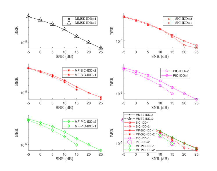
Figure 3: BER versus SNR for All APs and Centralized AP Selection varying number of IDD iterations with $L=32$, $K=8$

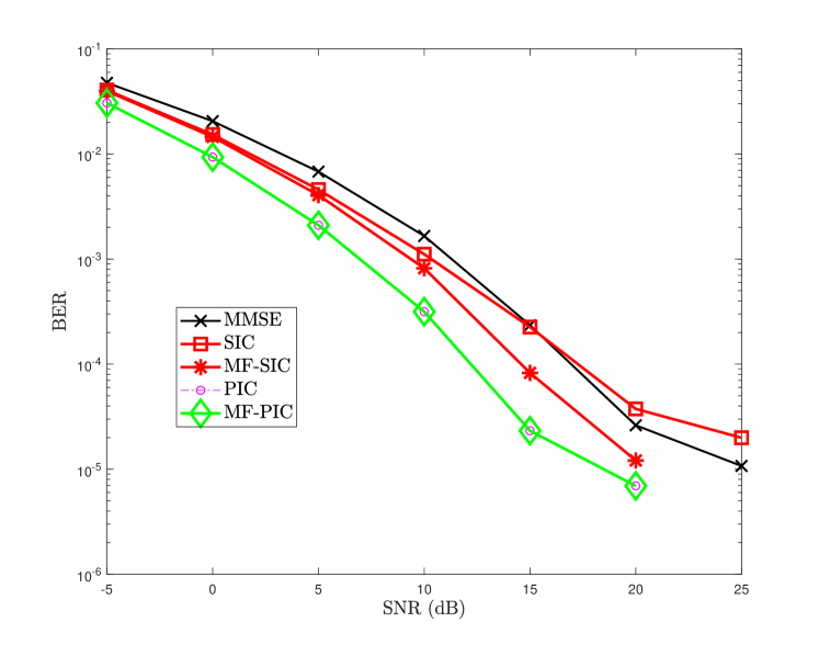
Figure 4: BER versus SNR for All APs and Centralized AP Selection with $L=32$, $K=8$, $\mathrm{IDD}=2$.

Figure 3 presents BER versus SNR as the number of IDD iterations are varied for (a) MMSE,(b) MMSE-Soft-IC and (c) List-MMSE-Soft-IC detection schemes. It can be observed that increasing number of iterations reduces the BER. This is because more a-posterior information is exchanged between the joint detector and decoder as the iterations increase, which improves the system performance. For the case of MMSE, the number of iterations do not reduce BER because there is no $\bm{\Delta}_{\text{i}}$ in this filter which is needed for the IDD scheme to improve the performance. Figure 4 presents the BER versus SNR for the case with APs selection and case when using all the APs while comparing the studied detectors. From this figure, It can be observed that the List-MMSE-Soft-IC detector achieves lower BER values, followed by the MMSE-Soft-IC detector and lastly the soft MMSE detector. Also the case with APs selection achieves slightly higher BER rates as compared to the case when all APs are used. This is due to reduction in diversity order.

VII Concluding Remarks

A joint list-based detector for CF-mMIMO architecture with centralized APs selection and processing is presented. Specifically, a new closed-form expression for the MMSE-soft-IC detection scheme with APs selection is derived. The resulting MMSE detectors are provided based on knowledge of the expectation of the transmitted symbols. More particularly, a list-based detector that can mitigate error propagation at the interference cancellation stage and enhance BER performance is proposed. Additionally, the soft MMSE and MMSE-Soft-IC detection techniques are contrasted with the suggested list-based detector. The performance of a system with and without APs selection is also compared. The system that uses all APs achieves lower BER values as compared to the one with APs selection. Thus, there is a trade-off between scalability and BER performance while using APs selection. The major advantage gained with APs selection is the reduction in the signaling between the APs and CPU which makes the network more scalable and practical.

References

- [1] R. C. de Lamare, ”Massive MIMO systems: Signal processing challenges and future trends,” in URSI Radio Science Bulletin, vol. 2013, no. 347, pp. 8-20, Dec. 2013.
- [2] W. Zhang et al., ”Large-Scale Antenna Systems With UL/DL Hardware Mismatch: Achievable Rates Analysis and Calibration,” in IEEE Transactions on Communications, vol. 63, no. 4, pp. 1216-1229, April 2015.
- [3] E. Björnson and L. Sanguinetti, ” Scalable Cell-Free Massive MIMO Systems”, IEEE Trans. Wireless Commun., vol. 68, no. 7, pp. 4247-4261, July 2020.
- [4] H. Q. Ngo, A. Ashikhmin, H. Yang, E. G. Larsson and T. L. Marzetta, ”Cell-Free Massive MIMO Versus Small Cells, ” IEEE Trans. Commun., vol. 16, no. 3, pp. 1834-1850, March 2017.
- [5] H. T. Dao and S. Kim, ” Effective channel gain-based access point selection in cell-free massive MIMO systems”, IEEE Access, vol. 8, pp. 108127 - 108132, June 2020.
- [6] V. M. T. Palhares, A. R. Flores and R. C. de Lamare, ”Robust MMSE Precoding and Power Allocation for Cell-Free Massive MIMO Systems,” in IEEE Transactions on Vehicular Technology, vol. 70, no. 5, pp. 5115-5120, May 2021
- [7] Shakya, I.L., Ali, F.H. ” Joint access point selection and interference cancellation for cell-free massive MIMO”, IEEE Commun. Lett., , vol. 25, no. 4, pp. 1313–1317, Apr. 2021.
- [8] Xiao-Yu Hu, E. Eleftheriou and D. M. Arnold, ”Regular and irregular progressive edge-growth tanner graphs,” in IEEE Transactions on Information Theory, vol. 51, no. 1, pp. 386-398, Jan. 2005.
- [9] C. T. Healy and R. C. de Lamare, ”Design of LDPC Codes Based on Multipath EMD Strategies for Progressive Edge Growth,” in IEEE Transactions on Communications, vol. 64, no. 8, pp. 3208-3219, Aug. 2016.
- [10] X. Wang and H. V. Poor, ” Iterative (turbo) soft interference cancellation and decoding for coded CDMA”, IEEE Trans. Commun., vol. 47, no. 7, pp. 1046–1061, Jul.1999.
- [11] M. Sellathurai and S. Haykin, ” TURBO-BLAST for wireless communications: Theory and experiments”, IEEE Trans. Signal Process., vol. 50, no. 10, pp. 2538–-2546, Oct. 2002.
- [12] A. G. D. Uchoa, C. T. Healy and R. C. de Lamare, ”Iterative Detection and Decoding Algorithms for MIMO Systems in Block-Fading Channels Using LDPC Codes,” in IEEE Transactions on Vehicular Technology, vol. 65, no. 4, pp. 2735-2741, April 2016
- [13] Z. Shao, R. C. de Lamare and L. T. N. Landau, ”Iterative Detection and Decoding for Large-Scale Multiple-Antenna Systems With 1-Bit ADCs, ” IEEE Wireless Commun. Lett., vol. 7, no. 3, pp. 476–479, Jun. 2018.
- [14] A. Matache, C. Jones and R. D. Wesel, ”Reduced complexity MIMO detectors for LDPC coded systems”, in Proc. IEEE Military Commun. Conf., Monterey, CA, USA, pp. 1073-1079, 31 Oct.-3 Nov. 2004.
- [15] R. C. De Lamare and R. Sampaio-Neto, ”Minimum Mean-Squared Error Iterative Successive Parallel Arbitrated Decision Feedback Detectors for DS-CDMA Systems,” IEEE Trans. Commun., vol. 56, no. 5, pp. 778–789, May 2008.
- [16] P. Li, R. C. de Lamare and R. Fa, ”Multiple Feedback Successive Interference Cancellation Detection for Multiuser MIMO Systems”, IEEE Trans. Commun., vol. 10, no. 8, pp. 2434–2439, Jun. 2011.
- [17] P. Li and R. C. De Lamare, ”Adaptive Decision-Feedback Detection With Constellation Constraints for MIMO Systems,” in IEEE Transactions on Vehicular Technology, vol. 61, no. 2, pp. 853-859, Feb. 2012
- [18] R. C. de Lamare, ”Adaptive and Iterative Multi-Branch MMSE Decision Feedback Detection Algorithms for Multi-Antenna Systems,” in IEEE Transactions on Wireless Communications, vol. 12, no. 10, pp. 5294-5308, October 2013.
- [19] P. Li and R. C. de Lamare, ”Distributed Iterative Detection With Reduced Message Passing for Networked MIMO Cellular Systems,” in IEEE Transactions on Vehicular Technology, vol. 63, no. 6, pp. 2947-2954, July 2014.
- [20] R. B. Di Renna and R. C. de Lamare, ”Iterative List Detection and Decoding for Massive Machine-Type Communications,” in IEEE Transactions on Communications, vol. 68, no. 10, pp. 6276-6288, Oct. 2020.
- [21] J. Liu and R. C. de Lamare, ”Low-Latency Reweighted Belief Propagation Decoding for LDPC Codes,” in IEEE Communications Letters, vol. 16, no. 10, pp. 1660-1663, October 2012
- [22] C. D’Andrea and E. G. Larsson, ”Improving Cell-Free Massive MIMO by Local Per-Bit Soft Detection, ” IEEE Commun. Lett., vol. 25, no. 7, pp. 2400–2404, Apr. 2021.