Adaptive Kalman Filtering with Exact Linearization and Decoupling Control on Three-Tank Process

Abstract

Water treatment and liquid storage are the two plants implementing the hydraulic three-tank system. Maintaining certain levels is the critical scenario so that the systems run as desired. To deal with, the optimal linear control and the complex advanced non-linear problem have been proposed to track certain dynamic reference. This paper studies those two using the combination of linearization and decoupling control under some assumptions. The result shows that the designed methods have successfully traced the dynamic reference signals. Beyond that, the adaptive system noise Kalman filter (AKF) algorithm is used to examine the estimation performance of the true non-linear system and the performance yields a rewarding prediction of the true system.

I Introduction

In the current industrial systems functioning either for liquid storage or flow treatment, hydraulic plant has becoming a big preference. This is due to the fact that chemical reactions would interfere those processes working around the desired performance so that maintaining the levels is a key requirement to reach certain goals. To deal with, various research has been proposed implementing a hydraulic mini-plant with divergent scenarios created in [1, 2] which is applied in this paper too, from the trivial linear under some desired points to the advanced uncertain non-linear systems approaching the true system as written in [3, 4] in general. The famed hydraulic system in [1] has been extensively studied among researcher in the field of optimal control and deterministic-based estimation. The decoupling constant observer is proposed in [5] to deal with FDI without fault estimation. As for the non-linear, the bi-linear approach Luenberger observer are studied by [6] and [7] regarding the leakage detection and the FDI using the cooperation of the likelihood ratio and the updated innovation over time respectively. Beyond that, the robust design of sliding mode scenario to estimate the fault with some occurrence of noises is written in [8]. In lie of advanced non-linear model, [9, 10] have developed array of decoupled estimators in the three-tank model for resulting the FDI residuals and for detecting the faults working around some various desired points in turn. In addition, modern fuzzy and NN control on the tanks have been studied by [11, 12, 13]. However, this deterministic scenarios ignores the uncertainties and disturbances of the system which could be ameliorated by its counterpart stochastic approach.

There have been several the well-known recursive classic Kalman techniques dealing with the non-linear problem, comprising from the extended, the unscented to the Gaussian Kalman filter [14]. Among those algorithms, the extended Kalman filtering (EKF) is a stochastic method being used to deal with the non-linear problem [15]. Due to the unknown stochastic-noise correlation in EKF leading to lack of mathematical corresponding between the Kalman-type output and the noise covariance, the critical proper choices of noises in both system-$\mathbf{Q}$ and measurement-$\mathbf{R}$ to obtain the desired performance working inside the error threshold are mathematically not fulfilled. To cope with, the two static and dynamic matrix mechanism have been proposed. This innovative matrix of system noise $\mathbf{Q}$ guarantee the full couple of variance and covariance but no literature has implemented this into the three-tank process. This is due to the fact that this dynamic-noise Kalman (AKF) is tremendously applied in the navigation (INS) and the positioning (GPS) by [16, 17, 18, 19].

Regarding the problem formulation, This paper is started with the mathematical description. Moreover, the linear control design and the non-linear with stabilization and exact linearization are studied in the following to examine the performance of reference tracking. Lastly, the innovative noise (AKF) algorithm is implemented to estimate the true system ended by some conlusion and future work related to the paper.

II Mathematical Descriptions

The proposed design of the three-tank hydraulic system is portrayed in Fig. (1). This dynamical system comprises three equal tanks with parallel cylindrical forms and also identical cross-sectional area of $A_{n}$, in which $\tau=3$ and $n=1,\dots,\tau$ such that $A_{1}=A_{2}=A_{3}$. Those three tanks are then linked with three-tube pipes, tank 1 and 3 $(\Phi_{1})$, tanks 3 and 2 $(\Phi_{3})$ along with the outflow part $(\Phi_{2})$, of the same cross-sectional area $\Phi_{n}\rightarrow\Phi_{1}=\Phi_{2}=\Phi_{3}$. However, the coefficients of outflow $(\mu_{ab})$ from the areas $\Phi_{n}$ are divergent, constituting $\mu_{13}=\mu_{32}\neq\mu_{20}$. Regarding the inputs, those tanks of 1 and 2 are driven by two DC-motor typed pumps with the flow rates of $q_{1}$ and $q_{2}$ in turn, denoted as flow per-rotation $m^{3}s^{-1}$ which should be controlled by arbitrary D/A (digital or analog) typed converter. Beyond that these pumps have the peak of flow rate $(\ast)$ for certain pump $m\rightarrow\forall m\in 1,2$, defining $q_{m}^{\ast}$. As for the observed level $(h_{n})$ variables, they are caught by the sensors of differential pressure piezo-resistive-typed transducer. This means those three levels are converted in terms of the respective signals of voltage. Likewise, the peak level of certain tank is defined as $h_{n}^{\ast}$.

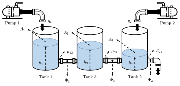
Figure 1: Three-tank hydraulic dynamical-system

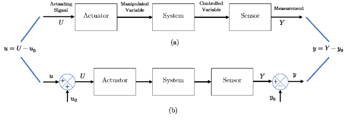
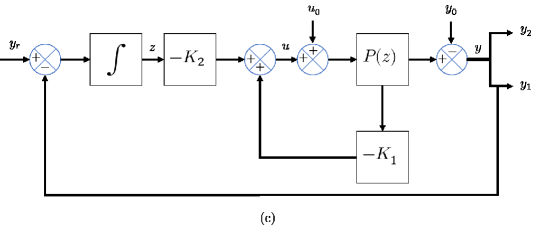
Figure 2: (a) The dynamic model representation taking into account the global operating points; (b) The linearized model representation considering the operating point $(u_{0},y_{0})$; (c) The basic nominal tracking control concept working around the operating point $(u_{0},y_{0})$

Furthermore, the cumulative mass rate $M_{t}$ in a system is corresponding to the difference mass rate of the inlet $M_{i}$ and the outlet $M_{o}$ (Bernoulli’s), therefore,

$$\frac{dM_{t}}{dt}=M_{i}-M_{o}$$ (1)

which could be changed into the more complex form related to certain fluid $(\rho_{n})$ being used in the system, such that

$$A\dot{h}=\rho q_{i}-\rho q_{o}$$ (2)

Since the fluid is even with the water, this means $\rho_{1}=\rho_{2}=\rho_{3}$ and the volume for each tank is dependent on the deviation of the cumulative inflow $(j)$ and outflow $(k)$,

$$A_{n}\frac{dh_{n}}{dt}=\sum_{j\in\mathcal{N}}(q_{i})_{n}-\sum_{k\in\mathcal{N}}(q_{o})_{n}$$ (3)

where for certain inflow apart from the two input-pump, the flow rate is denoted as $q_{ab}$, comprising outlet from tank $a$ to the inlet flow of tank $b$ with $a,b=1,\dots,\tau\rightarrow\forall a\neq b$, which is according to the law of Torricelli as written in the following formula, therefore

$$q_{ab}(t)=\mu_{ab}\Phi\operatorname{sign}(h_{a}(t)-h_{b}(t))\sqrt{2g|h_{a}(t)-h_{b}(t)|}$$ (4)

and the only outflow of the system is represented as,

$$q_{20}(t)=\mu_{20}\Phi\sqrt{2gh_{2}(t)}$$ (5)

From the whole preceding description being mentioned, the hydraulic mass balance non-linear system taking into account Eq. (3-5) is then written in the following equations,

$$A\frac{dh_{1}(t)}{dt} =q_{1}(t)-q_{13}(t)$$ (6a)

$$A\frac{dh_{2}(t)}{dt} =q_{2}(t)+q_{32}(t)-q_{20}(t)$$ (6b)

$$A\frac{dh_{3}(t)}{dt} =q_{13}(t)-q_{32}(t)$$ (6c)

II-A Linear Representation

A linear design of the system is then constructed assuming $h_{1}>h_{3}>h_{2}$ working in the equilibrium value of $(u_{0},y_{0})$ applying the Taylor expansion. The linearized LTI-discrete system with certain time sampling $t_{s}$ is denoted as,

$$\left\{\begin{aligned} x(k+1)&=A_{d}x(k)+B_{d}u(k)\\ y(k)&=Cx(k)\end{aligned}\right.$$ (7)

where the state $x\in\mathcal{R}^{n}$,

$$F=\begin{bmatrix}-\dfrac{\mu_{13}\Phi\varphi}{2A\sqrt{y_{01}-y_{03}}}&0&\dfrac{\mu_{13}\Phi\varphi}{2A\sqrt{y_{01}-y_{03}}}\\[10.00002pt] 0&-\dfrac{\mu_{13}\Phi\varphi}{2A\sqrt{y_{01}-y_{03}}}-\dfrac{\mu_{20}\Phi\varphi}{2A\sqrt{y_{02}}}&\dfrac{\mu_{32}\Phi\varphi}{2A\sqrt{y_{03}-y_{02}}}\\[10.00002pt] -\dfrac{\mu_{13}\Phi\varphi}{2A\sqrt{y_{01}-y_{03}}}&\dfrac{\mu_{32}\Phi\varphi}{2A\sqrt{y_{03}-y_{02}}}&-\dfrac{\mu_{32}\Phi\varphi}{2A\sqrt{y_{03}-y_{02}}}+\dfrac{\mu_{13}\Phi\varphi}{2A\sqrt{y_{01}-y_{03}}}\end{bmatrix};B=\begin{bmatrix}\dfrac{1}{A}&0\\[7.5pt] 0&\dfrac{1}{A}\\[7.5pt] 0&0\end{bmatrix}$$ (8)

along with the input $u\in\mathcal{R}^{m}$ and the output $y\in\mathcal{R}^{q}$ constituting the diverse of the equilibrium $(u_{0},y_{0})$. The whole dynamic in the form of state-space representation is formulated in Eq. (8) with $\varphi=\sqrt{2g}$. This so-called the operating point should be initially opted because there has been a related yield between the designed linearized model and the connection of the dynamic result of the system output and input working around the chosen operating point $(u_{0},y_{0})$. Suppose a system portrayed in Fig. (2a) with certain input $U$ and output $Y$, the linearized model working around the equilibrium point is shown in Fig. (2b), such that

$$u=U-u_{0}\qquad\textrm{and}\qquad y=Y-y_{0}$$ (9)

II-B Nominal Tracking Control Law

According to [20], the law of tracking control says that the number of controlled variables $\psi_{y}$ should be less than or equal to that of control inputs $\psi_{u}$ for the whole dynamical system $(\psi_{y}\leq\psi_{u})$. Otherwise, the desired variables must be selected among available states to track the reference $y_{r}$ as depicted in Fig. (2c). Since there are two inputs from those pumps $(q_{1},q_{2})$, the output is then designed as follows,

$$y(k)=\begin{bmatrix}y_{1}(k)\\ y_{2}(k)\end{bmatrix}=\begin{bmatrix}C_{1}\\ C_{2}\end{bmatrix}x(k)\longrightarrow y_{1}=\begin{bmatrix}h_{1}&h_{2}\end{bmatrix}^{T}$$ (10)

where the rest $y_{2}=h_{3}$ and $y_{1}\in\mathcal{R}^{p}$ with $p\leq m$ leading to achieve the steady-state $y_{r}-y_{1}=0$, thanks to the designed control, guaranteeing the dynamic performance of the system along with the stability. To reach the objective, a pair of comparator and its counterpart the integrator is implemented, satisfying

$$z_{m}(k+1)=z_{m}(k)+t_{s}\left(y_{r,m}(k)-y_{1,m}(k)\right)$$ (11)

where $y_{1}=C_{1}x$, $z\in\mathcal{R}^{p}\rightarrow z=\begin{bmatrix}z_{1}&z_{2}\end{bmatrix}^{T}$ and the definition of integrator in Fig. (2c) is presented in Eq. (11) as portrayed in Fig. (3). Keep in mind the proper set of the sampling time $t_{s}$ is vital, otherwise it leads to be unstable.

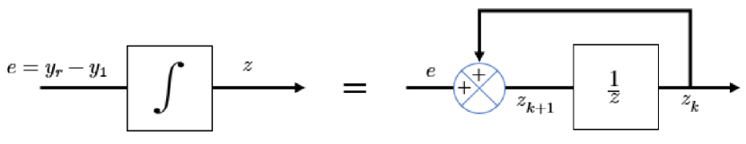
Figure 3: Integrator definition on Fig. (2c)

Moreover, the augmented state due to additional definition of $z$ is proposed as written below,

$$\left\{\begin{aligned} \begin{bmatrix}x(k+1)\\ z(k+1)\end{bmatrix}=&\begin{bmatrix}A_{d}&\textbf{O}_{n,p}\\ -t_{s}C_{1}&I_{p}\end{bmatrix}\begin{bmatrix}x(k)\\ z(k)\end{bmatrix}+\begin{bmatrix}B_{d}\\ \textbf{O}_{p,m}\end{bmatrix}u\\ &+\begin{bmatrix}\textbf{O}_{n,p}\\ t_{s}I_{p}\end{bmatrix}y_{r}\\ y(k)=&\begin{bmatrix}C&\textbf{O}_{q,p}\\ \end{bmatrix}\begin{bmatrix}x(k)\\ z(k)\end{bmatrix}\end{aligned}\right.$$ (12)

with $I_{v}$ acts as the $v$-dimensional identity matrix whereas the $\textbf{O}_{n,p}$, for instance, is the null-matrix of $n$-order rows and $p$-order columns. For the simplicity, the state-space in Eq. (12) is denoted as Eq. (13), such that

$$\left\{\begin{aligned} x_{e}(k+1)&=\bar{A}_{d}x_{e}(k)+\bar{B}_{d}u(k)+B_{r}y_{r}(k)\\ y(k)&=\bar{C}x_{e}(k)\end{aligned}\right.$$ (13)

and the feedback control could be calculated as in Eq. (14) using the classical pole placement technique being defined $\lambda$ as the desired eigenvalues.

$$u(k)=-Kx_{e}(k)=-\begin{bmatrix}K_{1}&K_{2}\end{bmatrix}\begin{bmatrix}x(k)\\ z(k)\end{bmatrix}$$ (14)

II-C Non-linear Decoupling Control Law

The system in Eq. (7) could be then elaborated as the non-linear model as written in the following model,

$$\left\{\begin{aligned} \dot{x}(t)&=\Delta(x(t))+\sum_{i=1}^{m}\xi_{i}(x(t))u_{i}(t),\quad m\in[1,2]\\ y(t)&=H(x(t))\end{aligned}\right.$$ (15)

and $\Delta(x(t))$ equals to $F$-matrix in Eq. (8) regardless the operating points, meaning the states $x$ relative to certain state $x_{i},\forall i\in n$ contain other states $x_{j},j<n$, making the preceding static $F$ into the dynamic over time instant $t$ whereas $\xi_{i}$ is the column vector of $B$-matrix or $B^{T}_{i}$, such that

$$\Delta(x(t))=\frac{1}{A}\begin{bmatrix}-q_{13}(t)\\ q_{32}(t)-q_{20}(t)\\ q_{13}(t)-q_{32}(t)\end{bmatrix}\quad\xi=\begin{bmatrix}\frac{1}{A}&0&0\\[2.5pt] 0&\frac{1}{A}&0\end{bmatrix}^{T}$$ (16)

Since this non-linear dynamic scenario has parallel objective as the preceding linear system, tracking certain reference signal $(y_{r})$, the exact linearization with decoupled control applying a constant feedback $u=\alpha(x)+\beta(x)\zeta$ is proposed to cope with it. This is also assumed that the dynamic has the same order of input-output $(q=m)$. To start with, supposed a set of respected degree for each row in Eq. (15) as $\vartheta_{i},\forall i\in m$,

$$\vartheta_{i}=\left\{\min l\in\mathsf{N}/\exists j\in\left[1:m\right],L_{\xi_{j}}L_{\Delta}^{l-1}H_{i}(x)\neq 0\right\}$$ (17)

where $L$ is the operator of Lie derivative so that $L_{\Delta}H_{i}(x)$, spoken as the Lie derivative of certain $H_{i}$ along $\Delta$ direction, comprises the derivative of such $H_{i}$ with respect to $t=0$ in the $\Delta$ integral curve, therefore

$$L_{\Delta}H_{i}(x)=\sum_{j=1}^{n}\Delta_{j}(x)\frac{\partial H_{i}}{\partial x_{j}}(x)$$ (18)

Lie $(L)$ operation for arbitrary direction $\epsilon$ for instance could be also iteratively defined with respect to any $k\geq 0$, such that

$$\left\{\begin{aligned} L_{\Delta}^{0}H(x)&=H(x)\\ L_{\Delta}^{k}H(x)&=L_{\Delta}\left(L_{\Delta}^{k-1}H(x)\right),\quad\forall k\geq 1\end{aligned}\right.$$ (19)

and if the variable $\vartheta_{i},\exists\,\forall i\in\left[1:m\right]$, the given variable $\Lambda$ is known as the decoupling matrix of Eq. (15),

$$\Lambda=\begin{bmatrix}L_{\xi_{1}}L_{\Delta}^{\vartheta_{1}-1}H_{1}(x)&\dots&L_{\xi_{m}}L_{\Delta}^{\vartheta_{1}-1}H_{1}(x)\\ \vdots&\ddots&\vdots\\ L_{\xi_{1}}L_{\Delta}^{\vartheta_{m}-1}H_{m}(x)&\dots&L_{\xi_{m}}L_{\Delta}^{\vartheta_{m}-1}H_{m}(x)\end{bmatrix}$$ (20)

where

$$\Lambda_{0}(x)=\begin{bmatrix}L_{\Delta}^{\vartheta_{1}}H_{1}(X)\\ \vdots\\ L_{\Delta}^{\vartheta_{m}}H_{m}(X)\end{bmatrix}$$ (21)

Having said the definition of $\vartheta_{i}$ in Eq. (17) along its existence $(\forall i\in m)$ leading to the decoupling $\Lambda$, further consideration follows with respect to non-linear design [21]. Firstly, the non-linear dynamic in Eq. (15) is decoupled on certain subset of $\Pi$ with $\mathcal{R}^{n}$ dimension, if the rank of $\Lambda(x)$ in Eq. (20) strictly equals to $m,\forall x\in\Pi$. Secondly, the non-linear feedback method is denoted as,

$$u(t)=\underbrace{-\Lambda^{-1}(x)\Lambda_{0}(x)}_{\alpha(x)}+\underbrace{\Lambda^{-1}(x)}_{\beta(x)}\zeta(t)$$ (22)

with $\zeta(t)$ defines the input vector of such respected linearized model and lastly, the performance of input-output relation of such closed-loop system is linear being defined as,

$$y_{i}^{(\vartheta_{i})}(t)=\zeta_{i}(t),\quad\forall i\in[1:m]$$ (23)

constituting the $\vartheta_{i}^{\rm{th}}$ derivative of certain $y_{i}$. Keep in mind that the magnitudes of $\vartheta_{i},\forall i\in m$, the closed-loop design could be represented as $m$-independent first-order of input-output system, on par with the integrator denoted as follows

$$\frac{h_{1}(s)}{\zeta_{1}(s)}=\frac{h_{2}(s)}{\zeta_{2}(s)}=\frac{1}{s}$$ (24)

with the unique of Laplacian $(s)$ variable. Furthermore, since $\sum_{i}^{n}\vartheta_{i}=2$ which is less than $n=3$, the stability needs to examine in the tank 3 as the unobservable subspace. However, this unobservable state has a stable performance so that the law of linearized control is implementable to this three-tank dynamical model. By contrast, If $\sum_{i}^{n}\vartheta_{i}=n$, the $m$-decoupling system comprises the linear property along with strict controllability and observability.

Due to each independent system in Eq. (24) is unstable, the further layer of decentralized control is applied using a proportional gain $(K_{i})$ from the output feedback, such that

$$\zeta_{i}(t)=K_{i}\left(y_{r,i}(t)-h_{i}(t)\right),\quad\forall i\in m$$ (25)

where it is on par with that of in the following,

$$\frac{h_{i}(s)}{y_{r,i}(s)}=\frac{K_{i}}{s+K_{i}}$$ (26)

Those two control scenarios are portrayed in Fig. (4b) with the detail of control blocks in Fig. (4c) for the stabilized and Fig. (4d) for the linearized control to maintain $y_{r}$.

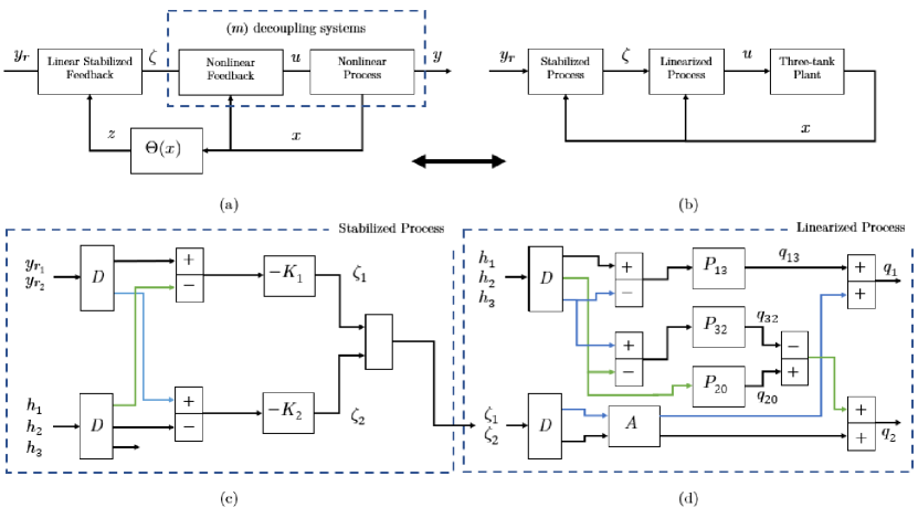
Figure 4: (a) The basic control law of non-linear system; (b) The generalized non-linear control fault-free scenario; (c) The stabilized block diagram for non-linear dynamical system; (d) The linearized block diagram for non-linear dynamical system

III Adaptive Covariance Kalman Filter

This paper proposes the adaptive covariance from the conventional centralized Kalman filter (CKF) from the dynamic in Eq. (8) as written in [23], therefore

$$\mathbf{F}_{k|k-1}=\left.\frac{\partial\mathbf{f}_{e}(\mathbf{x},\mathbf{u}_{k})}{\partial\mathbf{x}}\right|_{\mathbf{x}=\mathbf{x}_{k-1}}$$ (27)

where $\mathbf{f}_{e}(\mathbf{x},\mathbf{u}_{k})$ equals $A_{d}\mathbf{x}+B_{d}\mathbf{u}_{k}$ and the CKF is

$$\hat{\mathbf{x}}_{k}^{+} =\mathbf{f}_{e}\left(\hat{\mathbf{x}}_{k-1},\mathbf{u}_{k}\right)$$ (28a)

$$\mathbf{P}_{k}^{+} =\mathbf{F}_{k|k-1}\mathbf{P}_{k-1}\mathbf{F}_{k|k-1}^{\top}+\mathbf{Q}_{k-1}$$ (28b)

$$\mathbf{K}_{k} =\mathbf{P}_{k}^{+}\mathbf{H}^{\top}\left[\mathbf{H}\mathbf{P}_{k}^{+}\mathbf{H}^{\top}+\mathbf{R}_{k}\right]^{-1}$$ (28c)

$$\hat{\mathbf{x}}_{k} =\hat{\mathbf{x}}_{k}^{+}+\mathbf{K}_{k}\left(y_{k}-\mathbf{H}\hat{\mathbf{x}}_{k}^{+}\right)$$ (28d)

$$\mathbf{P}_{k} =\left(\mathsf{I}-\mathbf{K}_{k}\mathbf{H}\right)\mathbf{P}_{k}^{+}$$ (28e)

where $\mathbf{F}$ represents the linearized model whereas $\mathbf{P}^{+}$ and $\mathbf{P}$ constitute the covariance matrix of extrapolation and state-estimation error. Moreover, $\mathbf{K},\mathbf{R},\mathbf{I}$ are the respected gain of Kalman, the known covariance matrix of measurement noise along with the respected identity matrix of $\mathcal{R}^{n}$. The adaptive covariance matrix of process noise $\mathbf{Q}$ is iteratively designed using the following formula with the known $\mathbf{R}$ [22],

$$\hat{\mathbf{C}}_{\mathbf{v}_{k}}=\frac{1}{\Psi}\sum_{i=i_{0}}^{k}\mathbf{v}_{i}\mathbf{v}_{i}^{\top}\quad\longrightarrow\quad\mathbf{v}_{k}=y_{k}-\mathbf{H}\hat{\mathbf{x}}_{k}$$ (29)

with $\mathbf{v}_{k}$ denotes as the residual updated of the CKF and $i_{0}$ equals to $k-\Psi+1$ stating the initial sample of the estimated range of $\Psi$. The updated covariance matrix is formulated as,

$$\hat{\mathbf{Q}}_{k}=Q_{\alpha}+\mathbf{P}_{k}-\mathbf{F}_{k|k-1}\mathbf{P}_{k-1}\mathbf{F}_{k|k-1}^{\top}$$ (30)

where $\Delta\mathbf{x}_{k}=\hat{\mathbf{x}}_{k}-\hat{\mathbf{x}}_{k}^{+}$. Furthermore, the design in Eq. (30) could be approached with the steady assumption of the following formula, such that

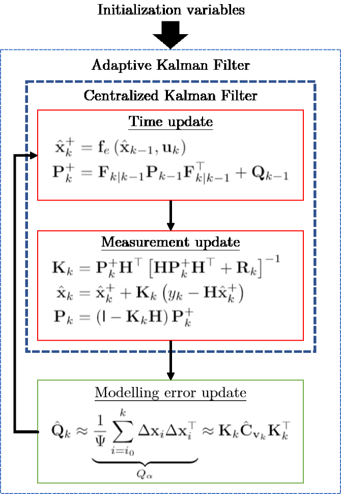
Figure 5: The adaptive $\mathbf{Q}$ algorithm (AKF) from the CKF

$$\hat{\mathbf{Q}}_{k}\approx\underbrace{\frac{1}{\Psi}\sum_{i=i_{0}}^{k}\Delta\mathbf{x}_{i}\Delta\mathbf{x}_{i}^{\top}}_{Q_{\alpha}}\approx\mathbf{K}_{k}\hat{\mathbf{C}}_{\mathbf{v}_{k}}\mathbf{K}_{k}^{\top}$$ (31)

Beyond that, the stability properties of system identification are well-described in [24], [25]. The ideas lie in the boundedness of $\mathbf{Q}$ and $\mathbf{R}$ under some constant scales ranging $(q^{-},q^{+})$ and $(r^{-},r^{+})$ respectively. Moreover, a non-singular $A_{d}$ and $\mathbf{H}$ must satisfy the observability and $\mathbf{P}_{0}$ must be strictly positive $(\mathbf{P}_{0}>0)$. The scale $(q^{-},q^{+})$ is greater than $0$ so that the boundedness of the Riccati equation is solved through $q^{-}\times I\leq\mathbf{P}\leq q^{+}\times I,\forall k\geq 0$.

IV Numerical Simulation Results

There are three major simulations presented in this chapter. For the dynamics, the parameters being used in the process are written in Table. (I) with $t_{s}=1s$ under some assumptions as in chapter (II-B).

Table I: Three-tank process parameters

Variable	Symbol	Value
CSA∗ of tank	A	0.0154 $m^{2}$
CSA∗ of inter-tank	$\Phi$	$5\times 10^{-5}$ $m^{2}$
Coefficient of outflow	$\mu_{13}=\mu_{32}$	0.5
Coefficient of outflow	$\mu_{20}$	0.675
Peak of flow-rate	$q_{m}^{\ast}(m\in[1,2])$	$1.2\times 10^{-4}$ $m^{3}s^{-1}$
Peak of level	$h_{n}^{\ast}(n\in[1:\tau])$	0.62 $m$
∗Note: CSA means cross-sectional area

This scenario is to control the dynamic of the plant working in the chosen operating point of $(u_{0},y_{0})$,

$$\begin{aligned} u_{o}&=\begin{bmatrix}0.35\times 10^{-4}&0.375\times 10^{-4}\end{bmatrix}^{\top}(m^{3}/s)\\ y_{o}&=\begin{bmatrix}0.40&0.20&0.30\end{bmatrix}^{T}(m)\end{aligned}$$

with certain design of the eigenvalues $(\lambda)$ of the extended matrix $A_{d}$ so that the feedback gain $(K_{i},\forall i\in m)$ in Fig. (2) is obtained in the following,

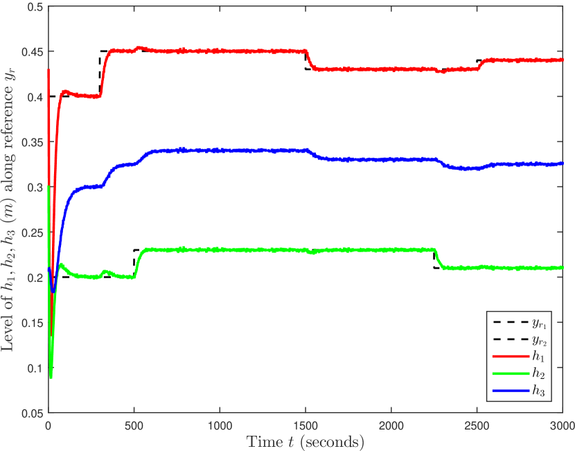
(a)

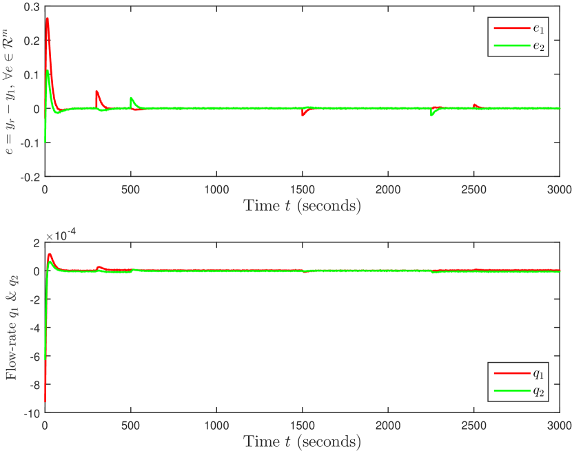
(b)

Figure 6: (a) The tracking performance of the linear control law over some dynamic references; (b) The error $(e_{i})$ and the control input $(q_{i})$ of the respected level

$$\lambda =\begin{bmatrix}0.92&0.97&0.90&0.95&0.94\end{bmatrix}$$

$$\begin{bmatrix}[c|c]K_{1}&K_{2}\end{bmatrix} =10^{-4}\times\begin{bmatrix}[ccc|cc]21.6&3&-5&-0.95&-0.32\\ 2.9&19&-4&-0.30&-0.91\end{bmatrix}$$

The findings are shown in Fig. (6) regarding the effectiveness of the linear control design $y$-coloured with respect to the dynamic step-reference $y_{r}$-black-dashed. This MIMO process has on par $(m=2)$ input-output relation, referring to the tank $i,\forall i\in m$ such that $h_{1}\rightarrow y_{r,1}$ and $h_{2}\rightarrow y_{r,2}$ working around the desired $(u_{0},y_{0})$. From the graph in Fig. (6(a)) the control law traces both references $y_{r,i}$ correctly. Since the dynamic of both references is divergent in both levels, each change between them $(h_{i})$ is always affecting other level performance $(h_{j})$, proven by the slight amplitude. As for Fig. (6(b)), it demonstrates the error $(e_{i})$ of the respected references along with the control input of the operating pumps $(q_{i})$.

Regarding the non-linear performance as explained in chapter (II-C), the system comprises 2 desired outputs so that the degrees are $\vartheta_{1}$ an $\vartheta_{2}$ as in Eq. (17) with certain decoupled control $\Lambda(x)$. Since the rank of $\Lambda(x)=m$, the system could be decoupled requiring a further variable of $\Lambda_{0}(x)$, such that

$$\Lambda(x)=\begin{bmatrix}[cc]L_{\xi_{1}}x_{1}(t)&L_{\xi_{2}}x_{1}(t)\\ L_{\xi_{1}}x_{2}(t)&L_{\xi_{2}}x_{2}(t)\end{bmatrix}=\begin{bmatrix}[cc]\frac{1}{A}&0\\[2.5pt] 0&\frac{1}{A}\end{bmatrix}$$

$$\Lambda_{0}(x)=\begin{bmatrix}L_{\Delta}x_{1}(t)\\ L_{\Delta}x_{2}(t)\end{bmatrix}=\begin{bmatrix}-\frac{1}{A}q_{13}\\[2.5pt] \frac{1}{A}\left(q_{32}-q_{20}\right)\end{bmatrix}$$

along with the proposed linearized input as given below,

$$u(t)=\frac{1}{A}\begin{bmatrix}-q_{13}(x_{t})\\ q_{32}(x_{t})-q_{20}(x_{t})\end{bmatrix}+\begin{bmatrix}A&0\\ 0&A\end{bmatrix}\zeta(t)$$

The non-linear responses are illustrated in Fig. (7) along with the error $e_{i}$, input pumps $q_{i}$ and the input of certain linearized design $\zeta_{i}$, $\forall i\in m$. Likewise, the dynamic of the reference $(y_{r,i})$ are on par with that of the linear of the respected output $y_{i}$. The stabilized and linearized concept of feedback (complete decoupling) could handle the non-linear performance, meaning there is no influence due to the dynamic of the reference from other tanks. In addition, the white noise is larger induced in the output system.

As for the AKF, the initial parameters being used are in the following,

$$\mathbf{x}_{0}=\begin{bmatrix}0.9&0.55&0.5\end{bmatrix}^{\top}$$

$$\mathbf{P}_{0}=10\times I_{3}\quad\mathbf{Q}_{0}=10^{-12}\times I_{3}\quad\mathbf{R}_{0}=5^{2}$$

and the AKF performances are depicted in Fig. (8) regarding the estimates $(\hat{y})$ and the true $y$ in (8(a)) and the error for each level in (8(b)). Both figures indicate the rewarding result of the filtering to estimate the true levels.

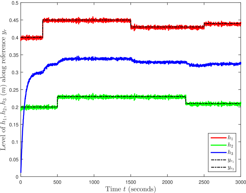
(a)

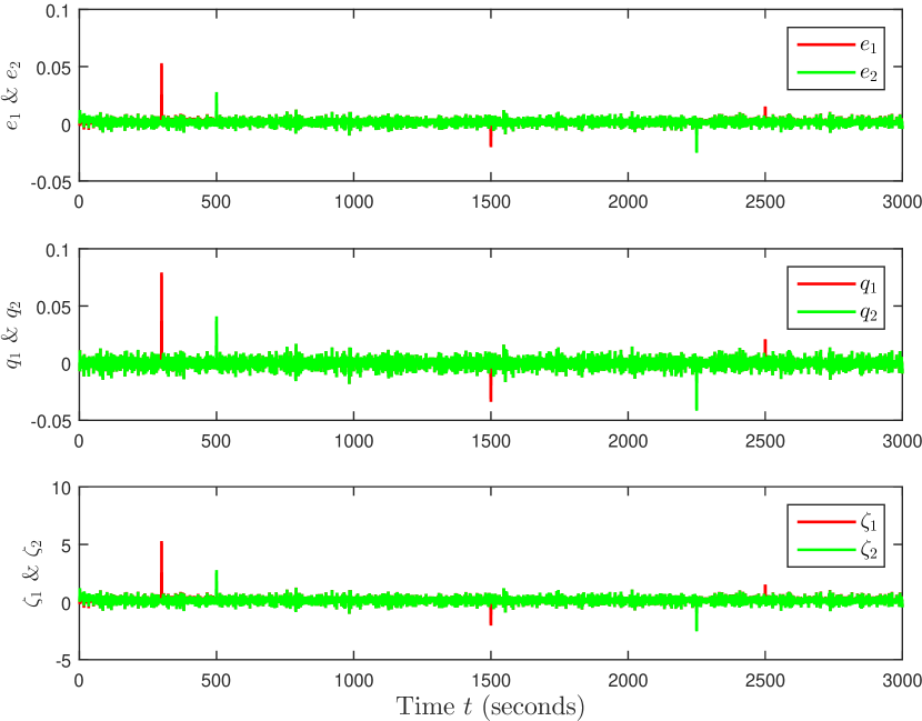
(b)

Figure 7: (a) The tracking performance of the non-linear control law with the stabilized and linearized decoupling control law over some dynamic references; (b) The error $(e_{i})$, the control input $(q_{i})$ and the equal linearized input $(\zeta_{i})$ of the respected level

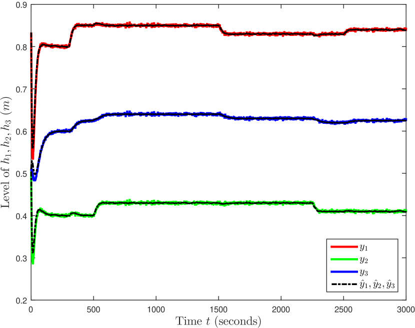
(a)

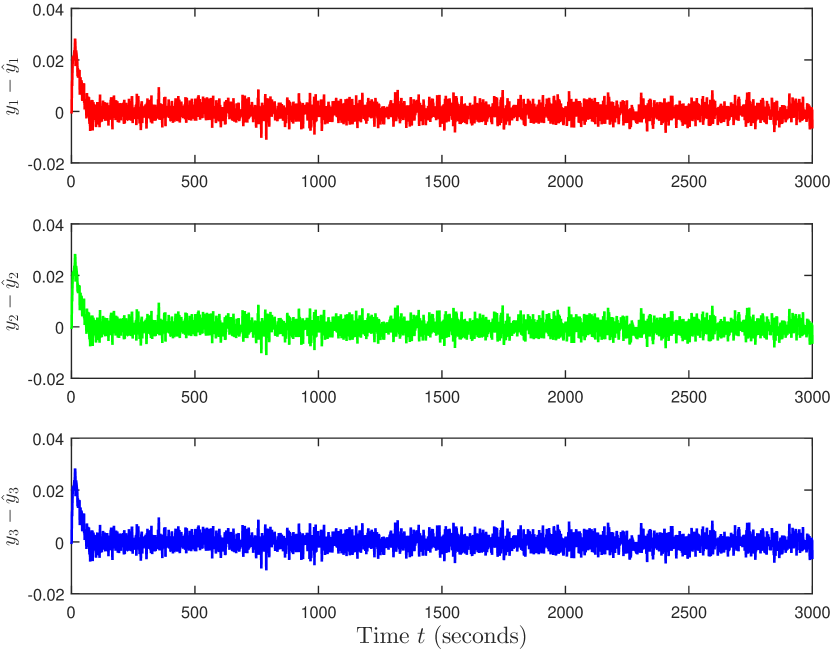
(b)

Figure 8: (a) The estimation performance $(\hat{y}_{i})$ of AKF over the output systems $(y_{i})$; (b) The estimation error $(\hat{e}_{i})$ from the true values of the respected level

V Conclusion

The mathematical design of three-tank has been formulated along with the state-feedback linear control and the non-linear law via constant feedback. Both scenarios have successfully tracked the dynamic reference signals $(y_{r})$ of tank 1 and 2. In addition, this paper also examine the effectiveness of the adaptive $(\mathbf{Q}_{k})$ filtering over non-linear cases and the performance yields the rewarding estimates over true states. For further research, the dynamic is more complex with some unobservable system (non-full rank) being tackled by the compressed sensing or $\ell_{0}$ norm method.

Authors

First and Correspondence Author - Moh Kamalul Wafi was graduated from the Imperial College London majoring Control Systems under Department of Electrical and Electronics Engineering. I am currently with the Laboratory of Embedded and Cyber-Physical Systems, Department of Engineering Physics, Institut Teknologi Sepuluh Nopember, 60111, Indonesia

References

- [1] Bismarckstr Amira GmbH. Documentation of the three-tank system. 65, D-47057 Duisburg, Germany, 1994
- [2] Noura, Hassan & Theilliol, Didier & Ponsart, Jean-Christophe & Chamseddine, Abbas. Fault-Tolerant Control Systems: Design and Practical Applications. 2009. 10.1007/978-1-84882-653-3.
- [3] R.A. Freeman and P.V. Kokotovic. Robust nonlinear control design: State-space and Lyapunov techniques. Birkh auser Boston, 2008. http://doi.org/10.1007/978-0-8176-4759-9
- [4] O. Gasparyan. Linear and nonlinear multivariable feedback control: A classical approach. Wiley, 2008
- [5] D. Koenig, S. Nowakowski, and T. Cecchin. An original approach for actuator and component fault detection and isolation. In 3rd IFAC Symposium on Fault Detection Supervision and Safety for Technical Processes, pages 97–107, Hull, UK, 1997
- [6] D.N. Shields and S. Du. An assessment of fault detection methods for a benchmark system. In 4th IFAC Symposium on Fault Detection Supervision and Safety for Technical Processes, pages 937–942, Budapest, Hungary, 2000
- [7] L. El Bahir and M. Kinnaert. Fault detection and isolation for a three-tank system based on a bilinear model of the supervised process. In United Kingdom Automatic Control Council International Conference on Control, volume 2, pages 1486–1491, Swansea, UK, 1998
- [8] J. Juan Rincon-Pasaye, R. Martinez-Guerra, and A. Soria Lopez. Fault diagnosis in nonlinear systems: an application to a three-tank system. In Proceedings of the IEEE American Control Conference, pages 2136–2141, Washington DC, USA, 2008.
- [9] A. Akhenak, M. Chadli, D. Maquin, and J. Ragot. State estimation via multiple observer with unknown inputs: application to the three-tank system. In 5th IFAC Symposium on Fault Detection, Supervision and Safety for Technical Processes, pages 1227–1232, Washington DC, USA, 2003
- [10] M. Rodrigues, D. Theilliol, M.A. Medina, and D. Sauter. A fault detection and isolation scheme for industrial systems based on multiple operating models. Control Engineering Practice, 16(2):225–239, 2008
- [11] J.M. Kohcielny. Application of fuzzy logic for fault isolation in a three-tank system. In 14th IFAC World Congress, pages 73–78, Beijing, R.P. China, 1999
- [12] C.J. Lopez and R.J. Patton. Takagi-sugeno fuzzy fault-tolerant control for a non-linear system. In Proceedings of the IEEE Conference on Decision and Control, pages 4368–4373, Phoenix, Arizona, USA, 1999
- [13] T. Marcu, M.H. Matcovschi, and P.M. Frank. Neural observer-based approach to fault-tolerant control of a three-tank system. In Proceedings of the European Control Conference, Karlsruhe, Germany, 1999. CD-Rom
- [14] S. C. Patwardhan, S. Narasimhan, P. Jagadeesan, B. Gopaluni, and S. L. Shah. Nonlinear bayesian state estimation: A review of recent developments. Control Engineering Practice, vol. 20, no. 10, pp. 933–953, August 2012.
- [15] F. Auger, M. Hilairet, J. Guerrero, E. Monmasson, T. Orlowska-Kowalska, and S. Katsura. Industrial applications of the Kalman filter: A review. IEEE Trans. Ind. Electron., vol. 60, no. 12, pp. 5458–5471, Dec. 2013.
- [16] C. Hide, T. Moore, and M. Smith. Adaptive Kalman filtering for low-cost INS/GPS. J. Navigat., vol. 56, no. 1, pp. 143–152, Jan. 2003.
- [17] D.-J. Jwo, F.-C. Chung, and T.-P. Weng. Adaptive Kalman Filter for Navigation Sensor Fusion. London, U.K.: IntechOpen, 2010.
- [18] A. Almagbile, J. Wang, and W. Ding. Evaluating the performances of adaptive Kalman filter methods in GPS/INS integration. J. Global Positioning Syst., vol. 9, no. 1, pp. 33–40, Jun. 2010
- [19] Wafi, Moh. (2019). Filtering module on satellite tracking. AIP Conference Proceedings. 2088. 020045. 10.1063/1.5095297.
- [20] J. D’Azzo and C.H. Houpis. Linear control system analysis and design, conventional and modern. McGraw-Hill Series in Electrical and Computer Engineering, 1995
- [21] H. Nijmeier and A.J. Van der Schaft. Nonlinear dynamical control systems. Springer, third edition, 1996.
- [22] A. H. Mohamed and K. P. Schwarz. Adaptive Kalman Filtering for INS/GPS. J. Geodesy, vol. 73, no. 4, pp. 193–203, May 1999.
- [23] S. S. Haykin. Kalman Filtering and Neural Networks. New York, NY, USA: Wiley, 2001
- [24] Wafi, Moh. (2021). Estimation and Fault Detection on Hydraulic System with Adaptive-Scaling Kalman and Consensus Filtering. International Journal of Scientific and Research Publications (IJSRP). 11. 49-56. 10.29322/IJSRP.11.05.2021.p11308.
- [25] Wafi, Moh. (2021). System Identification on the Families of Auto-Regressive with Least-Square-Batch Algorithm. International Journal of Scientific and Research Publications (IJSRP). 11. 65-72. 10.29322/IJSRP.11.05.2021.p11310.