Filtering Module on Satellite Tracking

Abstract

The scope of satellite has increasingly attained as one of the most challenging topics due to the attraction of elaborating the outer space. The satellite, as a means of collecting data and communicating, needs a proper calculation so as to maintain the movement and its appearance. The concept of the proposed research lies in the mathematical model along with certain noises. The mathematical model is started by initial two variable states, constituting a radius and an angle, with no process noise on it. These two states then are formulated with certain assumption of noises in terms of the range and the scaled angle deviations from them in turn. Keep in mind that those two noises are mutually independent and their covariance are considered. the model is defined as Algebraic Riccati Equation (ARE) along with Kalman filter algorithm, from the estimation, the steady-state estimator, the computational of gain matrix to the stability of the predictor. The findings show that, as for the two pairs of states, the performance of the estimation can follow the state with just slight fluctuations in the first a fifth of a thousand iterations. With respect to the Mean Square Error (MSE), both noises are around 0.2 for the four states.

I Introduction

Tracking an object is becoming more challenging and it has been studying to get the precise position while tracking it. The object refers to the satellite and it has increasingly attained as one of the most challenging topics due to the attraction of elaborating the outer space. The proposed concept of doing it is to use Kalman filter as conducted by [1] and [2] which presented the reduced order of the Riccati differential equation, the tractable of the object in terms of mathematical model, and the the ease in the real implementation in turn. This also stimulates to upgrade the classic Kalman filter in order to obtain another best estimation method as done by [3], comprising the upgrade of gradient decent in terms of error covariance. The classic Kalman filter [4] is emerged so as to compare the method in [7] in terms of the mean square estimation error (MSEE) along with its average over certain iterations.

The basic concept of the classic Kalman is set from [4] while the elaborating of the basic is well-presented in [6] saying the various possibility of any engineering and non-engineering being perturbed by any noises including tracking a moving object. The initial foundation has been inspired by [9], [4] along with [5] for the concept of filtering.

The classic is matched with the Micro-Kalman Filter developed by [7] which then was upgraded in the following paper presented in [8]. This algorithm is the beginning of the possibility of Distributed Kalman Filter (DKF). This paper proposes the algorithm compared to the classic in terms of the mean square error and overall performance of the states.

II Problem Formulation

This paper presents a mathematical modelling on satellite tracking as shown in Fig. 1 with the following qualitative objectives:

1. The problem is initiated from showing the right state-space in terms of nominally circular solution by considering small deviations of the state variables.

2. Those small deviations are measured in terms of observations on earth so that the two possible are suggested, the noisy measurements of both the range deviations from $R$ and the scaled angle deviations from $\omega t$.

3. The states estimation are derived either with or without initial condition with respect to both noises along with the mean square error (MSE)

III Mathematical Model

From the designed objectives, the basis construction of this paper is begun from the state-space itself with two additional deviations proposed. The following is to design the suitable Kalman filter with certain parameters related to the this paper.

III-A State-Space Representation

A unit human-made celestial body rotates in the subspace under the influence of an inverse square law force field. The motion of the mass is governed by a couple of second order differential equation for the ideal rotational move of radius $r(t)=R$ at time $t$

$$\ddot{r}(t)=r(t)\dot{\theta}^{2}-\frac{G}{r^{2}(t)}$$ (1)

$G_{0}$ is a physical constant enabling circular orbits being defined as $R^{3}\omega^{2}$ and that is also influenced by a certain angle $\theta(t)=\omega t$, such that:

$$\ddot{\theta}(t)=-2\dot{\theta}\frac{\dot{r}(t)}{r(t)}$$ (2)

To initiate the linearised equations about the nominally circular solution, the deviation $r$ from the ideal move has to be small and those are expressed as $\textbf{x}=\left[x_{1},x_{2},x_{3},x_{4}\right]^{T}$. The state variables, due to two pairs of $r$ and $\theta$, are defined as $x_{1},\cdots,x_{4}$, with $x_{1}=r-R$, $x_{2}=\dot{r}$, $x_{3}=R\left(\theta-\omega t\right)$, and $x_{4}=R(\dot{\theta}-\omega)$ in turn. Keep in mind that the process noise is ignored from the set linearised equations.

III-B The Construction of Noises

It is important to set two sorts of disturbances in measuring those two parameters $r$ and $\theta$ at sample times $t=kh$ with $k=1,2,\cdots,N$. The mean of such noise in terms of the range deviations from $R$ (type 1) is designed as zero whilst its covariance is known with certain parameter of $\varphi$, such that:

$$y_{1}\left(t\right)=x_{1}(t)+v_{1}(t)\rightarrow v_{1}\sim\mathcal{N}(0,\varphi)$$ (3)

Another noisy measurement is the scaled angle deviations from $\omega t$ (type 2) along with certain covariance of $\psi$:

$$y_{3}\left(t\right)=x_{3}(t)+v_{3}(t)\rightarrow v_{3}\sim\mathcal{N}(0,\psi)$$ (4)

$v_{1}$ is a Gaussian noise with mean $\hat{v}_{1}(0)=0$ and covariance $\mathcal{Q}_{v_{1}}(0)=\varphi$ whereas $v_{3}$ is equal to $\hat{v}_{3}(0)=0$ and $\mathcal{Q}_{v_{3}}=\psi$. Those two types affect the matrix of $H$ so that the the research is based on the two models leading to the different simulations.

III-C Kalman Estimation

The problems of estimating variables that are not directly available and without making any assumption on the stationary of the stochastic processes are addressed. Recalling the states of Kalman filter by taking into account $n$-vector process $x_{k}$ and $m$-vector process of observation $y_{k}$ generated by the following model, such that:

$$\hat{x}(kh) =Fx\left[\left(k-1\right)h\right]+u^{s}+q\left[\left(k-1\right)h\right]$$ (5)

$$\hat{y}_{1,3} =H\hat{x}(kh)+u^{0}+v_{1,3}\left[\left(k-1\right)h\right]$$ (6)

$q\sim\mathcal{W}\mathcal{G}\mathcal{N}(0,\delta)$ is a White Gaussian Noise with mean $\hat{q}_{1}(0)=0$ and covariance $\mathcal{Q}_{q}(0)=\delta$. The criteria is the same as that of for $y_{1,3}(kh)=Hx(kh)+u^{0}+v_{1,3}$, constituting $v_{1,3}\sim\mathcal{W}\mathcal{G}\mathcal{N}(0,\varphi\>\textrm{or}\>\psi)$ with equal $\hat{v}_{1,3}$ and $\mathcal{Q}_{v_{1,3}}$ which is non-singular. $q(\bullet)$ and $v_{1,3}(\bullet)$ are mutually independent with $x_{0}$ whereas $F,H,c^{T},V_{1}$, and $V_{2}$ are known. As an initial state, $x_{0}$, with Gaussian random, its mean and covariance are respectively written as:

$$E\left[x_{0}\right]=\hat{x}_{0|0}\quad\textrm{and}\quad\mathcal{Q}_{x}(0)=P_{0|0}$$ (7)

A prevalent of the steady-state filter aimed to either time-invariant or time-varying systems along with non-stationary noise covariance is time-varying Kalman filter. Bear in mind that the estimate of $\textbf{x}\left[(k-1)h|(k-1)h\right]$ is described as $\hat{\textbf{x}}\left[kh|(k-1)h\right]$ obtained from the preceding measurements with $y\left[(k-1)h\right]$ whereas the updated estimate according to the last measurement $y(kh)$ is explained as $\hat{\textbf{x}}\left[(kh|kh)\right]$. Note that the up-to-date estimate is $\hat{\textbf{x}}\left[(kh|kh)\right]$ and the iteration then predicts the following time-updated at $(k+1)h$. The measurement update hence employs this estimation according to the one-step-ahead predictor $y\left[(k+1)h\right]$ which then is used in the error term, the difference between the measured and estimated, defined by $y\left[(k+1)h\right]-c\hat{\textbf{x}}\left[(k+1)h|kh)\right]$. The innovation of gain $K$ is set to be minimum with respect to the covariance of the estimation error, such that:

$$\xi(kh)=\textbf{E}\left[v_{1}(kh)v_{1}(kh)^{T}\right]$$ (8)

The expected value of the second type noise is also written as $\zeta(kh)=\textbf{E}\left[v_{3}(kh)v_{3}(kh)^{T}\right]$.

III-D Steady-State Gain Matrices

The equations to each time-step upgrade $K\left[(k+1)h\right]$ and $P\left[(k+1)h\right]$ entail the inversion of a matrix that, assuming a $n$-by-$n$ matrix, requires $O(n^{3})$ operation (in general) and hence the complexity enumeration of each iteration escalates with the cubic power of the dimension of the state vector. This would be practically very appealing to be able to replace the time-varying matrices $K\left[(k+1)h\right]$ and $P\left[(k+1)h\right]$ with constant $K(kh)$ and $P(kh)$ calculated off-line previously. It would obviously provide a rise to a sub-optimal predictor but would allow to handle in practice high-dimensional problems, so that:

$$\hat{\textbf{x}}\left[(k+1)h|kh\right]=F\textbf{x}\left[kh|kh\right]+Ke(kh)$$ (9)

with $e=y-\hat{y}$. The steady-state gain matrix is simply computed as common Kalman $K=FPH^{T}\left(HPH^{T}+\psi\right)^{-1}$. Moreover, the matrix $P=P(kh)=P\left[\left(k+1\right)\right]$ is a solution of the Algebraic Riccati Equation (ARE):

$$P=F\left[P-PH^{T}\left(HPH^{T}+\psi\right)^{-1}HP\right]F^{T}+\varphi$$ (10)

In case of multiple solutions of the ARE, it is necessary to choose the positive semi-definite one. Recalling the equations of the following steady-state Kalman predictor:

$$\hat{y}\left[(k+1)h|kh\right]=H\hat{\textbf{x}}\left[(k+1)h|kh\right]$$ (11)

If $K$ stabilizes $F-KH$, the solution of the ARE is stabilizing. However, this does not say anything about the existence of a positive (definite or semi-definite) solution of ARE. Then, it is worth asking under what conditions the recursive Riccati equation converges, that is, the ARE has (at least) one positive semi-definite solution and by recalling that $P$ is the state prediction error covariance matrix.

III-E Micro-Kalman Filter $\mu$KF

The algorithm is based on research conducted by [7] and [8] being called as information form which was then to examine the possibility of constructing the Distributed Kalman Filter (DKF). The state of the plant is the same as the classical, such that:

$$x_{k+1} =A_{k}x_{k}+B_{k}\vartheta_{k}$$ (12)

$$z_{k} =H_{k}x_{k}+\chi_{k}$$ (13)

the schemes of $\vartheta_{k}$ and $\chi_{k}$ are set as $\mathcal{W}\mathcal{G}\mathcal{N}$ with additional properties as in the following:

$$\textbf{E}(\vartheta_{k}\vartheta_{l}^{T}) =Q_{k}\bar{\delta}_{kl} \textbf{E}(\chi_{k}\chi_{l}^{T}) =R_{k}\bar{\delta}_{kl}$$ (14)

initial error covariance $P_{k}$ and an inverse-covariance matrix $\hat{S}$ are combined to obtain matrix $M$, such that:

$$S_{k}=H^{T}_{k}R^{-1}_{k}H_{k}$$ (15)

$$M^{-1}=(P^{-1}+S)$$ (16)

whereas matrix of $K$ is influenced by the $M$-matrix as follows:

$$K_{k}=M_{k}H^{T}_{k}R^{-1}_{k}$$ (17)

The equation of state estimation is then altered from the common $\hat{x}_{k}=\hat{x}_{k|k-1}+K_{k}(y_{k}-H\hat{x}_{k|k-1})$ to:

$$\hat{x}m =\hat{x}_{k|k-1}+M_{k}(H^{T}_{k}R^{-1}_{k}y_{k}-H^{T}_{k}R^{-1}_{k}H\hat{x}_{k|k-1})$$ (18)

$$\hat{x}_{k|k-1} =\bar{x}_{0}$$ (19)

from the equation, it can be also written as $\hat{S}$ and a new measurement $z_{k}=H^{T}_{k}R^{-1}_{k}y_{k}$

$$\hat{x}_{m}=\bar{x}+M_{k}(z_{k}-\hat{S}\bar{x})$$ (20)

compared to the classic Kalman filter, the prediction of $\hat{x}$ and $P$ are becoming the update of this $\mu$KF such that:

$$P^{+}_{k} =AM_{k}A^{T}+B\delta B^{T}$$ (21)

$$\bar{x}^{+} =A\hat{x}_{m}$$ (22)

The algorithm is another, not the sequence of the classical, method and is compared to classic (centralized) Kalman filter in terms of estimation error.

Algorithm 1 Filtering Module

  Assumption:

  $x_{0}\sim\mathcal{N}(\acute{x}_{0},\tau)$; $q\sim\mathcal{N}(\bar{q},\delta)$;$v_{1}\sim\mathcal{N}(\bar{v}_{1},\varphi)$; $v_{3}\sim\mathcal{N}(\bar{v}_{3},\psi)$

  Initialization:

  $x_{0}=\bar{x}_{0}$ and $P_{0}=\tau$

  for $j=1$ to $\phi$ do

     for $k=1$ to $N$ do

        1. Centralized Kalman Filter

$$\hat{x}_{k|k-1} =Fx_{k-1}+u^{s}$$

$$\hat{y}_{k|k-1} =H\hat{x}_{k|k-1}+u^{0}$$

$$P_{k|k-1} =FP_{k-1|k-1}F^{T}+\delta$$

$$T =HP_{k|k-1}H^{T}+\textrm{noise}\rightarrow\varphi\>\textrm{or}\>\psi$$

$$P_{k} =P_{k|k-1}-P_{k|k-1}H^{T}(T)^{-1}HP_{k|k-1}$$

$$K_{k} =P_{k|k-1}H^{T}(T)^{-1}$$

$$\hat{x}_{k} =\hat{x}_{k|k-1}+K_{k}(y_{k}-\hat{y}_{k|k-1})$$

$$M_{k} =(P^{-1}+\hat{S}_{k})^{-1}$$

$$\hat{x}_{m} =\bar{x}_{0}+M_{k}(\hat{z}_{k}-\hat{S}_{k}\bar{x}_{0})$$

$$P_{k}^{+} =FM_{k}F^{T}+B\delta B^{T}$$

$$\bar{x}^{+} =F\hat{x}_{m}$$

$$\beta_{k} =|x_{k}-\hat{x}_{k}|$$

$$\gamma_{k} =|x_{k}-\bar{x}^{+}_{k}|$$

     end for

     Mean Square Estimation Error (MSEE):

$$\kappa_{j} =\frac{1}{N}\sum_{1}^{N}\beta^{2} \Gamma_{j} =\frac{1}{N}\sum_{1}^{N}\gamma^{2}$$

  end for

  Averaged MSEE:

$$\Xi_{\kappa} =\frac{1}{\phi}\sum_{1}^{\phi}\kappa \Xi_{\Gamma} =\frac{1}{\phi}\sum_{1}^{\phi}\Gamma$$

TABLE I: The Mean Square Estimation Error (MSEE) $\Gamma_{k}$ with noise type 1 $v_{1}$

State $\bar{x}^{+}$	Iteration $\phi_{i}$
	1	2	3	4	5	6	7	8	9	10	Averaged
$x_{1}$	0.0012	0.0015	0.0010	0.0043	0.0019	0.0015	0.0014	0.0011	0.0016	0.0012	0.0017
$x_{2}$	0.0023	0.0023	0.0038	0.0043	0.0076	0.0048	0.0052	0.0041	0.0070	0.0061	0.0048
$x_{3}$	0.0120	0.0032	0.0040	0.1271	0.0101	0.0059	0.0088	0.0039	0.0082	0.0081	0.0191
$x_{4}$	0.0022	0.0034	0.0019	0.0075	0.0037	0.0022	0.0042	0.0030	0.0042	0.0037	0.0036

TABLE II: The Mean Square Estimation Error (MSEE) $\Gamma_{k}$ with noise type 2 $v_{3}$

State $\bar{x}^{+}$	Iteration $\phi_{i}$
	1	2	3	4	5	6	7	8	9	10	Averaged
$x_{1}$	0.0207	0.0365	0.0095	0.0202	0.0116	0.0150	0.0085	0.0163	0.0191	0.0117	0.0169
$x_{2}$	0.0232	0.0395	0.0065	0.0205	0.0114	0.0157	0.0074	0.0159	0.0208	0.0112	0.0172
$x_{3}$	0.0155	0.0180	0.0129	0.0073	0.0090	0.0080	0.0081	0.0100	0.0114	0.0084	0.0109
$x_{4}$	0.0514	0.0779	0.0240	0.0389	0.0251	0.0346	0.0183	0.0353	0.0419	0.0240	0.0371

IV Simulation Results

The initialization of the simulation is presented with the following parameters. Supposing $R=1,\,\omega=1,\,G_{0}=1$ for $k=1,\cdots,N$ with $N=1000$ in both types. Moreover, assume that the probability density of the state at the initial time $t=0$ is described in the following equations, such that:

$$x_{0}=[0.1,0,0,0]\sim\mathcal{N}\left(\acute{x},\tau\right)$$ (23)

where mean is $0$ and its covariance is $0.1\times I_{4\times 4}$. Recalling the matrix of the states $\left[x_{1},x_{2},x_{3},x_{4}\right]^{T}$, the one-step-ahead from those four states are defined as follows:

$$\dot{x}_{1} =\dot{r}\rightarrow x_{2}$$

$$\dot{x}_{2} =\ddot{r}\rightarrow 3\omega^{2}x_{1}+2\omega x_{4}$$

$$\dot{x}_{3} =R(\dot{\theta}-\omega)\rightarrow x_{4}$$

$$\dot{x}_{4} =R\ddot{\theta}\rightarrow-2\omega x_{2}$$

where it can be concluded that the matrix of A would be:

$$\begin{bmatrix}\dot{x}_{1}(t)\\ \dot{x}_{2}(t)\\ \dot{x}_{3}(t)\\ \dot{x}_{4}(t)\\ \end{bmatrix}=\underbrace{\begin{bmatrix}0&1&0&0\\ 3\omega^{2}&0&0&2\omega\\ 0&0&0&1\\ 0&-2\omega&0&0\\ \end{bmatrix}}_{\textbf{A}}\underbrace{\begin{bmatrix}x_{1}(t)\\ x_{2}(t)\\ x_{3}(t)\\ x_{4}(t)\\ \end{bmatrix}}_{\textbf{x}}$$ (24)

from those two types of noise, it is showed the matrices of $y_{1}$ and $y_{3}$ are $\left[1,0,0,0\right]$ and $\left[0,0,1,0\right]$ respectively along with divergent noises of $\varphi=0.1$ and a hefty $\psi=0.5$. It then determines the matrix $F$ and the row vector $c^{T}$ in the equations relating $x(kh)$ and $y(kh)$ to $x\left[\left(k-1\right)h\right]$ and the appropriate noise variable. The value of $F$ with $\Delta t=h=0.01$ for either types is written as follows:

$$F=\begin{bmatrix}1.0001&0.0100&0&0.0001\\ 0.0300&1.0000&0&0.0200\\ -0.0000&-0.0001&1&0.0100\\ -0.0003&-0.0200&0&0.9998\\ \end{bmatrix}$$ (25)

while the value of $c^{T}_{1}$ and $c^{T}_{2}$ is then described the same as that of $H$.

Figure 1(a) highlights the true and the estimated states along with the measurement of the $\mu$KF for those four states being perturbed by type 1 noisy measurement and their MSEE(s) are illustrated in Table I. The Figure 1(e) presents the error among the states in Figure 1. The comparison on Table III $(\textbf{type 1})$ says that the almost there is no gap between the $\mu$KF and the classic Kalman filter which highlights the different just a slight $10^{-4}\times[1,1,2,0]^{T}$. Whilst, in terms of the bigger noisy measurement type 2 with a hefty $0.5$, the patterns of result are the same as those of the preceding graphs with respect to MSEE and AMSEE which are no much different compared to the CKF shown in Table II and Table III respectively. Table III $(\textbf{type 2})$ portrays the $10^{-4}\times[4,3,6,10]^{T}$ compared to the classic. The error in Figure (red) 2(e) are the conclusion of the figure from 2(a) to 2(d) which have the bigger span due to the bigger error set.

TABLE III: AMSEE comparison of $\Xi_{\kappa}$ and $\Xi_{\Gamma}$ with either noises

State	type 1		type 2
	$\Xi_{\kappa}$	$\Xi_{\Gamma}$	$\Xi_{\kappa}$	$\Xi_{\Gamma}$
$x_{1}$	0.0017	0.0016	0.0169	0.0165
$x_{2}$	0.0048	0.0047	0.0172	0.0169
$x_{3}$	0.0191	0.0193	0.0109	0.0103
$x_{4}$	0.0036	0.0036	0.0371	0.0361

V Conclusion

The initial mathematical model of the classic and the micro has been proposed along with the construction of two noisy measurements. From the results, it can be concluded that $\mu$KF Kalman filtering is being able to track the satellite with mean square estimation error (MSEE) being shown in Table I and Table II perturbed by either noises. This algorithm results in almost exactly the same as classic Kalman filter as depicted in Table III.

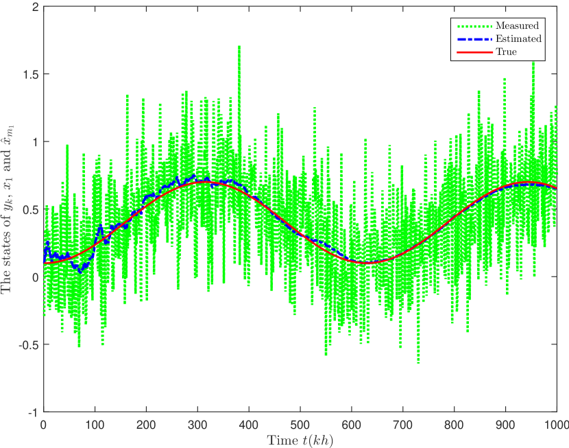
(a)

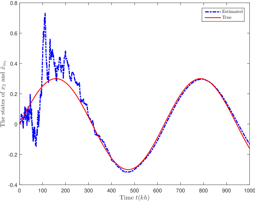
(b)

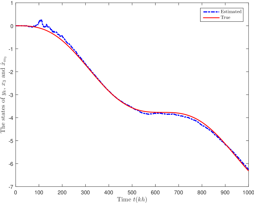
(c)

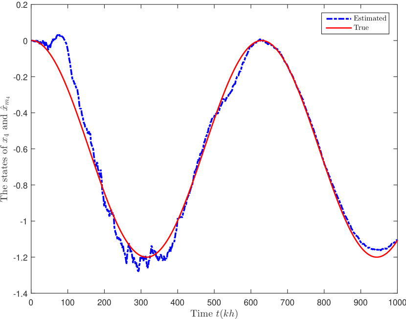
(d)

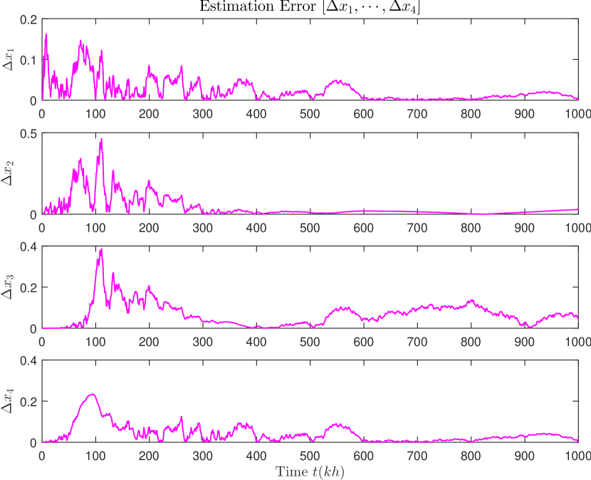
(e)

Figure 1: These figures present the results of the filtering according to four different states of position (a), velocity (b), angle (c), and angular velocity (d) whereas the last figure (e) portrays the error between the true and the estimated. The charts are influenced by noise type 1 whilst (a) is given additional information of measurement

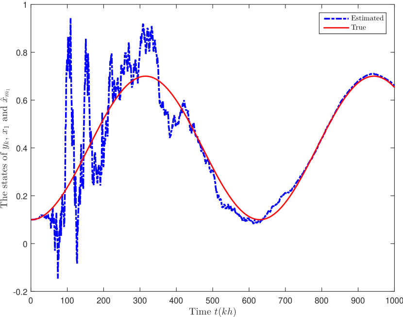
(a)

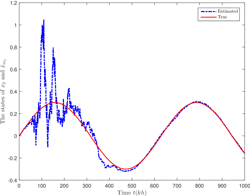
(b)

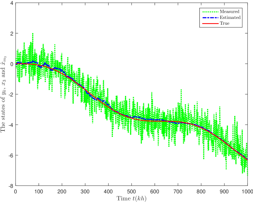
(c)

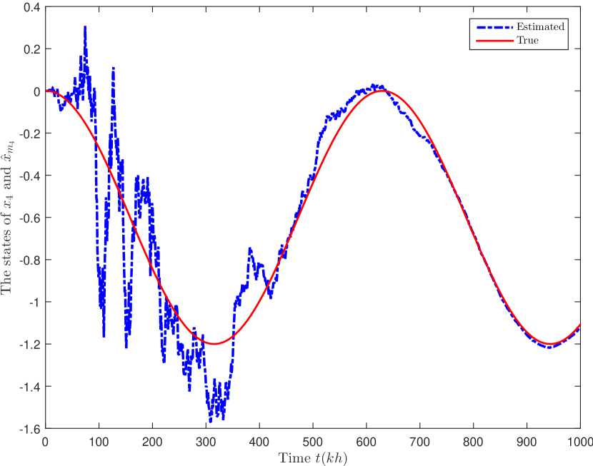
(d)

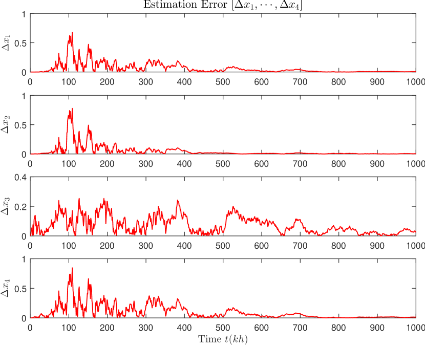
(e)

Figure 2: The following figures present the results of the filtering according to four different states of position (a), velocity (b), angle (c), and angular velocity (d) whereas the last figure (e) portrays the error between the true and the estimated. The charts are influenced by noise type 2 whilst (c) is given additional information of measurement

References

- [1] F. A. Faruqi and R. C. Davis, ”Kalman Filter Design for Target Tracking”, IEEE Transactions on Aerospace and Electronics Systems, Vol. AES-16, No. 4 July 1980
- [2] B. Esmat, ”An Adaptive Kalman Filter for Tracking Maneuvering Targets”, Journal of Guidance, Control, and Dynamics, September, Vol. 6, No. 5: pp. 414-416
- [3] W. Yuh-Shyang, S. You and N. Matni, ”Localized Distributed Kalman Filters for Large-Scale Systems”, ELSEVIER - IFAC Papers online, 50-1 (2017) 10742 - 10747
- [4] R. E. Kalman, ”A New Approach to Linear Filtering And Prediction Problems”, ASME Journal of Basic Engineering, 1960.
- [5] B. D. O. Anderson and J. B. Moore, Optimal Filtering. New York: Dover, 2005.
- [6] E. Mansour, ”Book Reviews” on Optimal Filtering, IEEE Transactions on Systems, Man, And Cybernetics, Vol. SMC-12, No. 2, March/April 1982.
- [7] R. Olfati-Saber, ”Distributed Kalman Filter with Embedded Consensus Kalman Filters”, Proceedings of the 44th IEEE Conference on Decision and Control, and the European Control Conference, Seville, Spain, Dec 12 - 15, 2005.
- [8] R. Olfati-Saber, ”Distributed Kalman Filtering for Sensor Networks”, Proceedings of the 46th IEEE Conference on Decision and Control, New Orleans, LA, USA, Dec. 12 - 14, 2007.
- [9] M B. Rhudy, R. A. Salguero and K. Holappa, ”A Kalman Filtering Tutorial for Undergraduate Students”, International Journal of Computer Science and Engineering Survey (IJCSES), Vol.8, No.1, February 2017.