High Speed Neuromorphic Vision-Based Inspection of Countersinks in Automated Manufacturing Processes

Abstract

Countersink inspection is crucial in various automated assembly lines, especially in the aerospace and automotive sectors. Advancements in machine vision introduced automated robotic inspection of countersinks using laser scanners and monocular cameras. Nevertheless, the aforementioned sensing pipelines require the robot to pause on each hole for inspection due to high latency and measurement uncertainties with motion, leading to prolonged execution times of the inspection task. The neuromorphic vision sensor, on the other hand, has the potential to expedite the countersink inspection process, but the unorthodox output of the neuromorphic technology prohibits utilizing traditional image processing techniques. Therefore, novel event-based perception algorithms need to be introduced. We propose a countersink detection approach on the basis of event-based motion compensation and the mean-shift clustering principle. In addition, our framework presents a robust event-based circle detection algorithm to precisely estimate the depth of the countersink specimens. The proposed approach expedites the inspection process by a factor of 10$\times$ compared to conventional countersink inspection methods. The work in this paper was validated for over 50 trials on three countersink workpiece variants. The experimental results show that our method provides a precision of 0.025 mm for countersink depth inspection despite the low resolution of commercially available neuromorphic cameras. Video Link

1 INTRODUCTION

Automation of manufacturing processes has been transforming the industrial landscape for over a century, beginning with Ford’s introduction of the assembly line. While automated manufacturing was initially aimed at producing large quantities, low-value, and standardized items karim2013challenges , it is now being applied to producing high-value, specialized items. This shift is driven by the need to achieve and sustain competitiveness in an operating environment with a growing number of competitors and declining highly specialized labor jayasekara2022level . In addition, automated manufacturing is becoming increasingly feasible due to the combination of low-cost computational power and the declining costs of sensors and actuators. This allows for more specialized applications to be realized across various industries, including aerospace and automotive assembly lines jayasekara2022level . These technologies are making it possible to create flexible, efficient, and lean automated manufacturing processes.

Automated industrial inspection is one of the essential operations in automated assembly lines, with computer vision being the driving force of the aforementioned process cim_survey ; inspection_jim_machinevision . Such fundamental operation suffices the objectives of safety and quality control, allowing industries to identify the potential faults of products and conduct corrective action accordingly. Therefore, industrial inspections demand precise scanning for complete, digital representation of mechanical parts. 3D scanning is widely used for geometric reconstruction, and automated aircraft inspections yasuda2022aircraft ; da20233d ; shahid_hybrid ; jim_auto_inspection . Different types of scanners with varied capabilities in terms of accuracy and portability have been developed for visual inspection in manufacturing. Kruglova et al. kruglova2015robotic developed a drone embedded 3D scanner for aircraft wing inspection. However, they reported challenges with achieving the required levels of precision. Sa et al. sa2018design developed visual measurement technology for counterbores based on laser sensors. Vision inspection is also being used in inspecting drilling holes in aircraft manufacturing with acceptable levels of accuracy 3d_csk_measurement . Other applications of computer vision in an inspection include: trajectory generation phan2018path and robot-attached 3D scanners for inspection and repair, respectively burghardt2017robot ; cladding .

Countersink inspection is a critical aspect of drilling and requires reliable and fast inspection methods for quality control. As such, it is important to integrate the inspection process into an automation system to achieve high production rates, enhanced quality control accuracy, and ensure traceability in real time integrated_hole . According to Luker et al. luker2020process , countersink depth, and the associated flushness of the fastener head is one of the challenging aspects to inspect and automate using computer vision approaches. The requirement for precise tolerance levels is restricted by the limitations of available laser scanning systems in terms of cost, and the lack of controlled industrial operating environments luker2020process . Furthermore, considering the wide adoption of countersinks in flush rivets of aircraft paneling, inspection for quality control significantly impacts the performance of riveted joints yu2019vision , imposing a surging demand for developing a reliable countersink inspection system.

Countersink inspection is mainly undertaken with the aid of two methods: non-contact and contact. The contact approach, basically the same as mechanical probing, is mainly used to determine the interior diameter of holes yu2019vision . The main challenge with the contact method is high susceptibility to loss of accuracy resulting from debris and cutting lube buildup nsengiyumva2021advances ; yu2019vision . Non-contact methods include laser sensors and machine vision, which are increasingly adopted with current industrial automation trends. Haldimann 3d_csk_measurement performed countersink inspection using digital light processing (DLP) projector and a monocular camera achieving a precision of 0.03 mm. In addition, Luker & Stansbudy luker2020process proposed using high-accuracy laser scanners to inspect countersinks, dropping the precision up to 6 $\mu m$. While these works provide the requirements of the current industrial requirements, they remain costly active methods and require extensive calibration and instrumentation. Therefore, Yu et al. yu2019vision utilized a high-resolution monocular camera for countersink inspection, while abiding by the industry’s requirements and attaining a precision of 0.02 mm. Nevertheless, such precision is conditional, given the imaging sensor is normal to the countersink specimens. To circumvent this limitation, Wang and Wang wang2016handheld utilized spectral domain optical coherence tomography (SD-OCT) for non-contact countersink inspection to deliver accurate countersink measurements without requiring precise scan center alignment.

Despite the growing adoption of computer vision for automated countersink inspection, the execution time of the inspection task was never taken into consideration. In all of the aforementioned methods, sensor motion during inspection is prohibited as it introduces measurement errors and degrades precision. This restriction results from the fact that laser scanners are associated with high latency and conventional cameras suffer from motion blur, leading to prolonged execution time of the inspection task. Neuromorphic vision sensors (NVS) address the limitations of the aforementioned sensing pipelines delineated by their low latency ($1\mu s$), high temporal resolution ($1ms$), and high dynamic range ($120$ dB), granting them robustness against motion blur and illumination variation vision_transformer ; davis . Unlike synchronous conventional cameras, the NVS generates asynchronous events as a response to variations of light intensity event_survey . This asynchronous nature triggered a paradigm shift in the computer vision community, as neuromorphic cameras unveiled their impact in space robotics nvbm_tim ; scramuzza_space ; space_debris , robotic manufacturing ayyad_drilling , robotic grasping flicker_grasp ; grasp_wong , autonomous navigation event_odometry_1 ; event_odometry_2 , tactile sensing yahya_tactile ; yahya_tactile_2 , and visual servoing hay2021unified .

1.1 Contributions

With the unprecedented capabilities of neuromorphic cameras in hand, this paper investigates the feasibility of high-speed neuromorphic vision-based inspection of countersinks. In the proposed framework, the NVS asynchronous nature is leveraged, where the sensor rather sweeps the countersinks on the mechanical part instead of pausing on each hole, reducing the inspection time to a few seconds. However, the NVS is an emerging technology and requires event-based perception algorithms for neuromorphic perception. Accordingly, this article comprises the following contributions to neuromorphic inspection of countersinks:

1. A novel event-based countersink detection algorithm is proposed based on motion compensation and the mean-shift clustering principle that overcomes the speed limitations of conventional countersink inspection methods.

2. A robust event-based circle detector is devised on the basis of Huber loss minimization to cope with the unconventional nature of the NVS and to provide the required inspection precision.

3. To validate the proposed inspection framework, we performed over 50 trials of an NVS sweeping three countersink workpieces with different hole sizes at speeds ranging from 0.05 to 0.5 m/s. The results show the inspection process is accelerated by a factor of 10$\times$ compared to state-of-the-art inspection methods while providing a precision of 0.025 mm with a low resolution NVS.

1.2 Structure of The Article

The rest of the article is organized as follows. Section 2 provides an overview of the neuromorphic vision working principle and an overview of the inspection setup. Section 3 discusses the theory behind the event-based motion compensation and event-based circle detection for countersink depth estimation. Experimental validation of the proposed inspection pipeline is reported in section 4, and section 5 presents conclusions and future works.

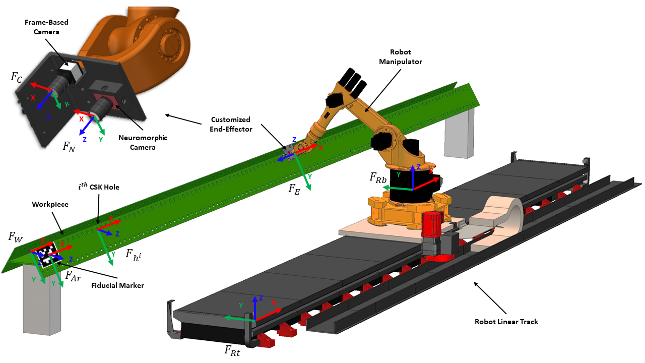
Figure 1: The robotic inspection setup illustrates the different components and defines the coordinate frames used for navigation and control.

2 Preliminaries

2.1 Robotic Inspection Setup

The overall setup of the neuromorphic vision-based inspection system can be seen in Figure 1. The presented system consists of an industrial robotic manipulator, and a customized end-effector holding a frame-based camera and a neuromorphic camera.

For the purpose of robot navigation and control, we have defined the following frames of reference:

• $\mathcal{F}_{Rb}$: The robot base coordinate frame.

• $\mathcal{F}_{Rt}$: The robot linear track coordinate frame.

• $\mathcal{F}_{E}$: The robot end-effector coordinate frame.

• $\mathcal{F}_{C}$: The frame-based camera coordinate frame.

• $\mathcal{F}_{N}$: The neuromorphic camera coordinate frame.

• $\mathcal{F}_{W}$: The workpiece coordinate frame.

• $\mathcal{F}_{Ar}$: The fiducial / ArUco coordinate frame.

• $\mathcal{F}_{h^{i}}$: The coordinate frame of the $i^{th}$ reference hole.

The rotation matrix mapping a source frame $\mathcal{F}_{S}$ to a target frame $\mathcal{F}_{T}$ can be defined as ${}_{T}R_{S}\in\mathbb{R}^{3\times 3}$. The position vector that gives the relative position of point b to point a described in $\mathcal{F}_{T}$ can be defined as ${}^{T}_{a}\vec{P}_{b}\in\mathbb{R}^{3}$. Then, we can define the affine transformation ${}_{T}T_{S}\in\mathbb{R}^{4\times 4}$ as follows:

$$_{T}T_{S}=\begin{bmatrix}{}_{T}R_{S}&{}^{T}_{T}\vec{P}_{s}\\ \mathbf{0}^{T}&1\end{bmatrix}$$ (1)

Using the robot’s forward kinematics relations, the affine transformation matrix ${}_{Rt}T_{E}$ can be identified and considered known for the remainder of this paper. The robot’s forward kinematics can be denoted as follows:

$$_{Rt}T_{E}=g(\theta),\hskip 14.22636pt\theta\in\mathbb{C}$$ (2)

where $\theta$ is the monitored angles of the robotic manipulator and linear track, $g(\theta)$ is a nonlinear function representing the robot’s kinematics, and $\mathbb{C}$ is the robot’s configuration space. Additionally, the constants ${}_{E}T_{C}$ and ${}_{E}T_{N}$ can be computed using the geometrical calibration method explained in ayyad2023neuromorphic . Hence, ${}_{B}T_{E}$ and the calibrated transformations can be utilized to solve for ${}_{B}T_{C}$ and ${}_{B}T_{N}$. Finally, we define the neuromorphic camera’s twist vector $\vec{V}_{N}=[v_{x},v_{y},v_{z},\omega_{x},\omega_{y},\omega_{z}]^{T}$ that represents the neuromorphic camera’s velocity in its own frame $\mathcal{F}_{N}$, where $[v_{x},v_{y},v_{z}]$ and $[\omega_{x},\omega_{y},\omega_{z}]$ are the linear and angular velocities respectively. The velocity components are computed from the forward kinematics of the robot manipulator as follows:

$$\vec{\mathcal{V}}_{N}=J(\theta)\dot{\theta}$$ (3)

$$J(\theta)\triangleq\dfrac{\partial g_{N}}{\partial\theta}\in\mathbb{R}^{6\times N_{j}}$$ (4)

where $J(\theta)$ is the Jacobian matrix of the camera’s forward kinematics function $g_{N}$, and $N_{j}$ is the number of robot joints.

As the major reference frames of the robotic setup are defined, the inspection routine is performed, with the neuromorphic camera sweeping the workpiece at a constant high speed. Prior to initiating the inspection process, the robot must first localize the workpiece in 6-DoF and align the neuromorphic camera accordingly. The robot starts with a priori estimate of the workpiece’s pose ${}_{Rt}\hat{T}_{W}$, and the pose of the fiducial marker ${}_{Rt}\hat{T}_{Ar}$. The robot then places the frame-based camera with a specific standoff away from the fiducial marker and utilizes the ArUco pose estimation method of the OpenCV library openCV to refine ${}_{Rt}\hat{T}_{Ar}$, similar to the approach used in halawani_visuo . Subsequently, the pose of each $i^{th}$ hole relative to the fiducial marker is known from the CAD model of the workpiece and is used to estimate the hole’s pose relative to the robot’s base frame:

$${}_{Rt}\hat{T}_{h^{i}}=\hskip 1.0pt_{Rt}\hat{T}_{Ar}\hskip 1.0pt{}_{Ar}T_{h^{i}},\hskip 14.22636pti\in[1,N_{h}]$$ (5)

Once the pose of each hole is estimated, the robot places the neuromorphic camera normal to the first hole with a specific relative pose and initiates the sweeping process. The sweeping process is performed by moving the neuromorphic camera with a constant velocity $\vec{V}_{N}^{*}$ across all the holes that lie in a straight line and have identical orientation. Given the position of the first hole ${}^{N}_{N}\vec{P}_{h^{1}}$ and last hole ${}^{N}_{N}\vec{P}_{h^{N_{h}}}$ described in $\mathcal{F}_{N}$, the linear components of $\vec{V}_{N}^{*}$ are computed as follows:

$$\begin{bmatrix}v^{*}_{x}\\ v^{*}_{y}\\ v^{*}_{z}\\ \end{bmatrix}=v^{*}\hskip 5.69046pt\frac{{}^{N}_{N}\vec{P}_{h^{N_{h}}}-^{N}_{N}\vec{P}_{h^{1}}}{||^{N}_{N}\vec{P}_{h^{N_{h}}}-^{N}_{N}\vec{P}_{h^{1}}||}$$ (6)

where $v^{*}$ is the desired magnitude of the sweeping speed. The rotational components of the sweeping motion are set to zero $[\omega^{*}_{x},\omega^{*}_{y},\omega^{*}_{z}]^{T}=\vec{0}$. The commanded camera velocity $\vec{V}_{N}^{*}$ is then transformed to command joint velocities $\theta^{*}$ by inverting the expression in (3), which are tracked using low-level PID controllers.

2.2 Neuromorphic Vision Sensor

The NVS is a bio-inspired technology that comprises an array of photodiode pixels triggered by light intensity variations. Upon activation, the pixels generate asynchronous events, where they are designated with spatial and temporal stamps as

$$e_{k}\doteq(\vec{x}_{k},t_{k},p_{k}),$$ (7)

where $(x,y)_{k}\in W\times H$ is the spatial stamp defining the pixel coordinates, $W\in\{1,...,w\}$ and $H\in\{1,...,h\}$ represent the sensor resolution, $t$ is the timestamp, and $p\in\{-1,+1\}$ is the polarity corresponding to a decrease and increase in light intensity, respectively.

While the NVS output is unorthodox in contrast with traditional imaging sensors, it is fundamentally important to point out that the NVS utilizes identical optics to conventional cameras. Thus, the neuromorphic sensor follows the standard perspective projection model expressed by

$$s\begin{bmatrix}u\\ v\\ 1\end{bmatrix}=\underbrace{\begin{bmatrix}f{x}&\gamma&u_{0}\\ 0&f_{y}&v_{0}\\ 0&0&1\end{bmatrix}}_{K}\underbrace{\begin{bmatrix}r_{11}&r_{12}&r_{13}&t_{1}\\ r_{21}&r_{22}&r_{23}&t_{2}\\ r_{31}&r_{32}&r_{33}&t_{3}\end{bmatrix}}_{R|\mathbf{t}}\begin{bmatrix}x\\ y\\ z\\ 1\end{bmatrix},$$ (8)

where $u$ and $v$ are the image coordinates of a mapped point in 3D space with world coordinates $x$, $y$, $z$, whereas $K$ is the intrinsic matrix comprising of the focal lengths $f_{x}$ and $f_{y}$, skew $\gamma$, and principal point $[u_{0},v_{0}]$. On the other hand, $R|t$ is the extrinsic parameters representing the transformation from world coordinates to the sensor frame.

3 Methodology

This section presents the event-based inspection pipeline of the countersink holes. As the NVS performs a quick sweep of the countersinks workpiece, the unconventional nature of the neuromorphic sensor permits utilizing conventional image processing techniques for inspection. Therefore, section 3.1 presents an event-based method for identifying the countersinks on the basis of motion compensation and mean-shift clustering. Finally, we propose a robust circle detection algorithm to estimate the depths of the countersink specimens with high precision, as described in section 3.2.

3.1 Event-Based Detection of Countersinks

As the neuromorphic vision sensor sweeps the workpiece, let the $N_{e}$ events in $e_{k}$ $\in$ $\mathbf{E}_{i}$ be the generated events when the sensor is normal to a designated countersink set. Since dealing with $\mathbf{E}_{i}$ in the space-time domain introduces undesired computational complexities, the events need to be transformed to a 2D space for lightweight feature extraction of the observed holes. A naive approach is to accumulate the events to 2D images directly from their spatial stamps $\vec{x}_{k}$. Nevertheless, large accumulation times are correlated with motion blur, while short accumulation periods lead to degraded features of the countersink specimens. To counteract these limitations, we rather adopt event-based motion compensation unifying_contrast ; moseg and leverage the asynchronous nature of neuromorphic events to create sharp images of warped events (IWE) defined by

$$H_{i}(\vec{x};\vec{\dot{U}})=\sum^{N_{e}}_{k}p_{k}\delta(\mathbf{x}-\vec{x}^{\prime}_{k}),$$ (9)

where

$$\vec{x}^{\prime}_{k}=\vec{x}_{k}-\vec{\dot{U}}(t_{k}-t_{i}).$$ (10)

Each pixel $\mathbf{x}$ in the IWE $H_{i}$ sums the polarities $p_{k}$ of the warped events $\vec{x}^{\prime}_{k}$ to a reference time $t_{i}$ given a candidate optical flow $\vec{\dot{U}}=[\dot{u},\dot{v}]^{T}$, where $t_{i}$ is the initial timestamp of $\mathbf{E}_{i}$ and $\delta$ is the dirac delta function. As discussed in section 2.1, the inspection involves a fixed countersinks workpiece, while the NVS twist vector $\vec{V}_{N}$ and the workpiece depth $Z$ are known as a priori. Therefore, $\vec{\dot{U}}$ can be computed using the image jacobian $\mathbf{J}$ handbook as

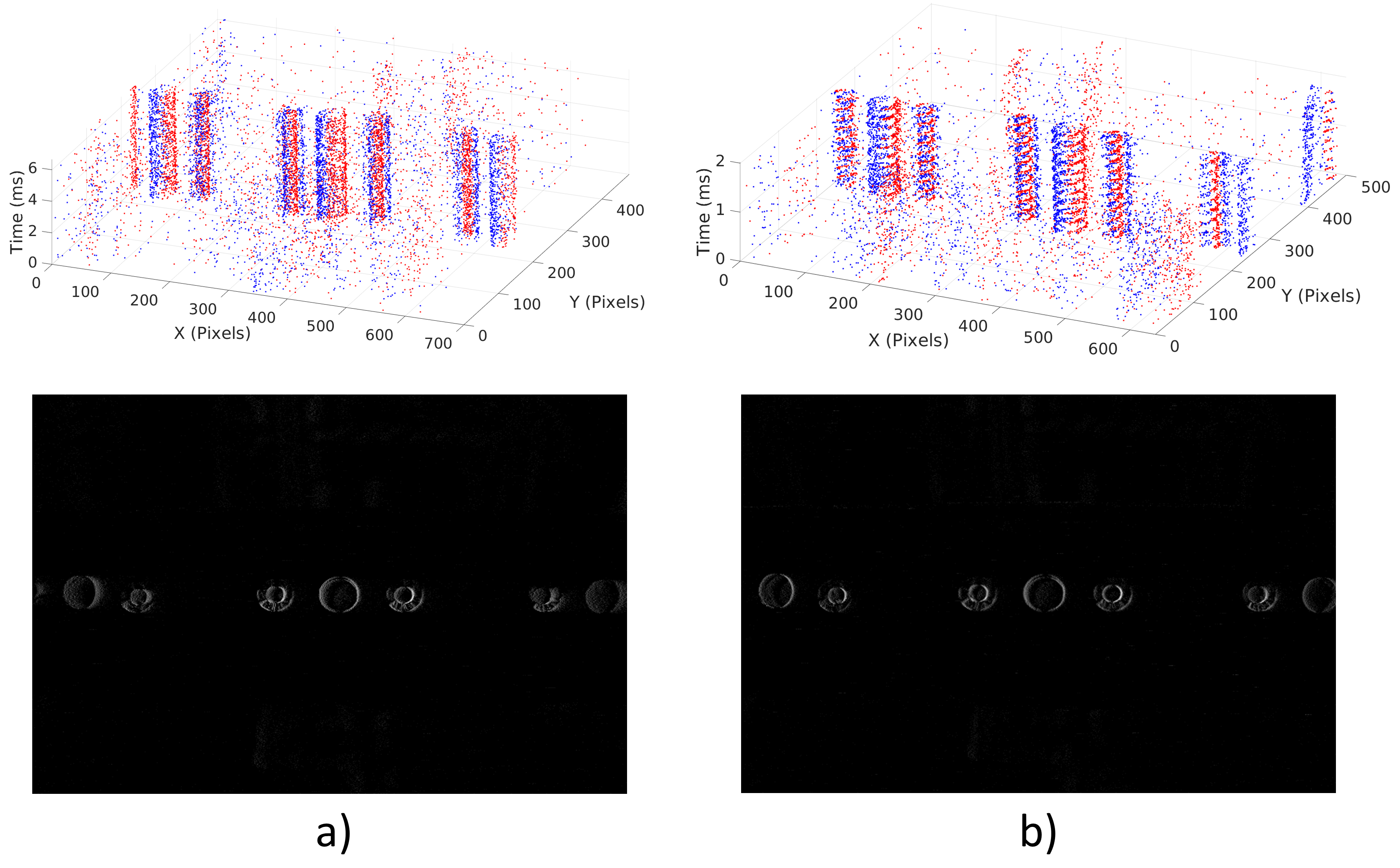
Figure 2: a) The raw event stream and the constructed $H_{i}$ at 0.05 m/s, and b) presents the raw event stream and $H_{i}$ at 0.5 m/s. Both IWEs are textured regardless of the NVS velocity.

$$\vec{\dot{U}}=\underbrace{\begin{bmatrix}\frac{-F}{Z}&0&u/Z&uv/F&-(F+u^{2}/F)&v\\ 0&\frac{-F}{Z}&v/Z&F+v^{2}/F&-uv/F&-u\end{bmatrix}}_{\mathbf{J}}\vec{V}_{N},$$ (11)

where $F$ is the focal length and $[u,v]$ are the pixel coordinates. We constrain the NVS motion during the sweep to 2D linear motion reducing the expression in (11) to $\dot{u}=\frac{-F}{Z}v_{x}$ and $\dot{v}=\frac{-F}{Z}v_{y}$. Having $\vec{\dot{U}}$ expressed in closed form, $H_{i}$ is simply constructed at each timestep $i$. It is worth mentioning that in our approach, $\mathbf{E}_{i}$ comprises of at least $N_{e}=10000$ events to create a textured $H_{i}$ regardless of its time step size. Figure 2 shows the raw event stream along with the obtained $H_{i}$ at speeds of 0.05 and 0.5 m/s. Notice that the quality of the IWEs is maintained regardless of the sensor speed.

After constructing $H_{i}$, an opening morphological transformation morph is applied to remove background noise, and the remaining activated pixels of warped events $e^{\prime}$ are what we call the surface of active events (SAE). To identify the normal countersinks set present in $H_{i}$, $e^{\prime}$ is fed to unsupervised mean-shift clustering algorithm mean_shift with a tunable bandwidth $\beta$ and a flat kernel $\mathcal{K}(e^{\prime})$ defined by

$$\mathcal{K}(e^{\prime})=\frac{1}{2}\begin{cases}1,&\text{if }-1\leq|G|\leq 1\\ 0,&\text{otherwise,}\end{cases}$$ (12)

and

$$G=|\frac{e^{\prime}-e_{k}}{\beta}|\text{ },\text{where }i=1,2,\cdots,N_{e}.$$ (13)

Given $\mathcal{K}(e^{\prime})$, $l_{1}\cup l_{2}\cup\cdots\cup l_{L}$ mutually exclusive clusters are obtained by optimizing the clustering parameters, as illustrated in mean_shift . Since multiple countersinks are observed at time step $i$, the normal countersinks to be inspected correspond to the cluster $\mathbf{L^{*}}$ closest to the principal point expressed by

$$\mathbf{L^{*}}=\operatorname*{arg\,min}_{L}||\vec{W}_{l}-\begin{bmatrix}u_{0}\\ v_{0}\end{bmatrix}||_{2},$$ (14)

where $\vec{W}_{l}$ are the centroids of the clustered activated events $e^{\prime}_{l}$. Figure 3 shows the mean-shift clustering performance on a pilot hole and two nut-plate installation holes.

Figure 3: Identified countersinks for nut-plate installation holes during the inspection using the mean-shift clustering principle. The left and right countersinks are highlighted in blue and green, respectively. The red points represent the pilot hole.

3.2 Depth Estimation of Countersink Holes

After identifying the $l^{*}$ countersinks, their inner and outer radii need to be evaluated for depth estimation. Nevertheless, conventional circle detectors such as the circle Hough transform (CHT) and edge drawing-circles (ED-Circles) edge_drawing ; ed_circles are not applicable as an edge image is obtained with the absence of the gradient. Therefore, we devise a nonlinear robust least squares problem, as described in Algorithm 1 to jointly cluster $e^{\prime}_{l}$ to either edge of the countersink and optimize the fitting parameters $\Gamma$, comprising of the circle inner $r$ and outer $R$ radii, and its image point center $h$ and $k$.

Given initial fitting parameters $\mathbf{\gamma}^{*}=[r,R,h,k]_{0}^{T}$, $e^{\prime}_{l}$ is first transformed to polar coordinates $\vec{x}_{r}=||\vec{x^{\prime}}_{l}-[h,k]_{0}^{T}||_{2}$, where $\vec{x^{\prime}}_{l}$ are the spatial stamps of $e^{\prime}_{l}$. Consequently, $\vec{x^{\prime}}_{l}$ is clustered with hard data association by

$$\vec{x}^{i}_{r}=\operatorname*{arg\,min}_{r^{*}}||\vec{x}_{r}-r||_{2}\\$$ (15)

where $\vec{x}^{i}_{r}$ are the activated events corresponding to the inner edge of the, while the rest of the events are otherwise. It is fundamentally important to highlight that the clustering in expression 15 is done at each optimization step. By jointly optimizing the clustering along with the fitting parameters, the expected likelihood of $e^{\prime}_{l}$ probability density function is maximized, ensuring robust data association.

Finally, the residual vector $\vec{\xi}$ is formulated with the euclidean distance between the clustered $\vec{x}_{r}$ in 15 and $\gamma^{*}$ by

$$\vec{\xi}=\begin{bmatrix}(\vec{X}^{i}-h_{0})^{2}+(\vec{Y}^{i}-k_{0})^{2}-r^{2}\\ (\vec{X}^{o}-h_{0})^{2}+(\vec{Y}^{o}-k_{0})^{2}-R^{2}\end{bmatrix},$$ (16)

where $\vec{X}^{i}$ and $\vec{Y}^{i}$ are the spatial stamps of $\vec{x}^{i}_{r}$, while $\vec{X}^{o}$ and $\vec{Y}^{o}$ are the spatial stamps of $\vec{x}^{o}_{r}$.

Utilizing ordinary least squares (OLS) to optimize $\Gamma$ can be affected by the presence of outliers. It is evident in Figures 2 and 3 that the countersink circular edge is accompanied by Gaussian noise. While utilizing weighted least squares with a normally distributed weighting vector can alleviate this restriction, reflections also appear on the inner walls of the holes, degrading the aforementioned approach’s performance. Instead of minimizing the sum of the squared residuals, a Huber loss function huber is utilized to penalize the impact of outliers. The Huber loss $\alpha(\vec{\xi})$ is formulated as

$$\alpha(\vec{\xi})=\begin{cases}\vec{\xi}^{2},&\text{if }|\vec{\xi}|\leq 1\\ 2\vec{\xi}-1,&\text{otherwise,}\end{cases}$$ (17)

and is fed to the Levenberg–Marquardt (LM) lm algorithm to optimize $\Gamma$ obtained as

$$\Gamma=\begin{bmatrix}r\\ R\\ h\\ k\\ \end{bmatrix}=\operatorname*{arg\,min}_{\Gamma^{*}}\sum_{l}\alpha(\vec{\xi}),$$ (18)

where the optimization is initialized with initial condition $\gamma^{*}$ parameterized by the mean of the inner $r_{0}$ and outer radii $R_{0}$, and the centroid of $\vec{x}_{l}$. Figure 4 shows the circle fitting using Huber loss and is compared to fitting using OLS on nut-plate installation holes. Notice that the fitting is robust against the noise and reflection outliers, unlike the linear loss of OLS.

Inputs : $e^{\prime}_{l}\in l^{*}$

Data: $Z$, $\phi$

Output : $\Gamma=[r,R,h,k],Z^{\prime}$

Initialize $\gamma^{*}=[r_{0},R_{0},h_{0},k_{0}]^{T}$

for $l=1$ to $l^{*}$ do

       while Not Converged do

             Transform $\vec{x}_{l}$ to $\vec{x}_{r}=||\vec{x^{\prime}}_{l}-[h,k]_{0}^{T}||_{2}$

             Cluster $\vec{x}_{r}$ to $\vec{x}_{r}^{i}$ and $\vec{x}_{r}^{o}$ , Equation 15

             Find $\vec{\xi}$ and $\alpha(\vec{\xi})$ , Equations 18 and 17

             Step $\Gamma$

       end while

      Find $r_{m}$ and $R_{m}$, Equation 19

       Inspect $Z^{\prime}$, Equation 20

end for

Algorithm 1 Depth Estimation of Countersink Holes

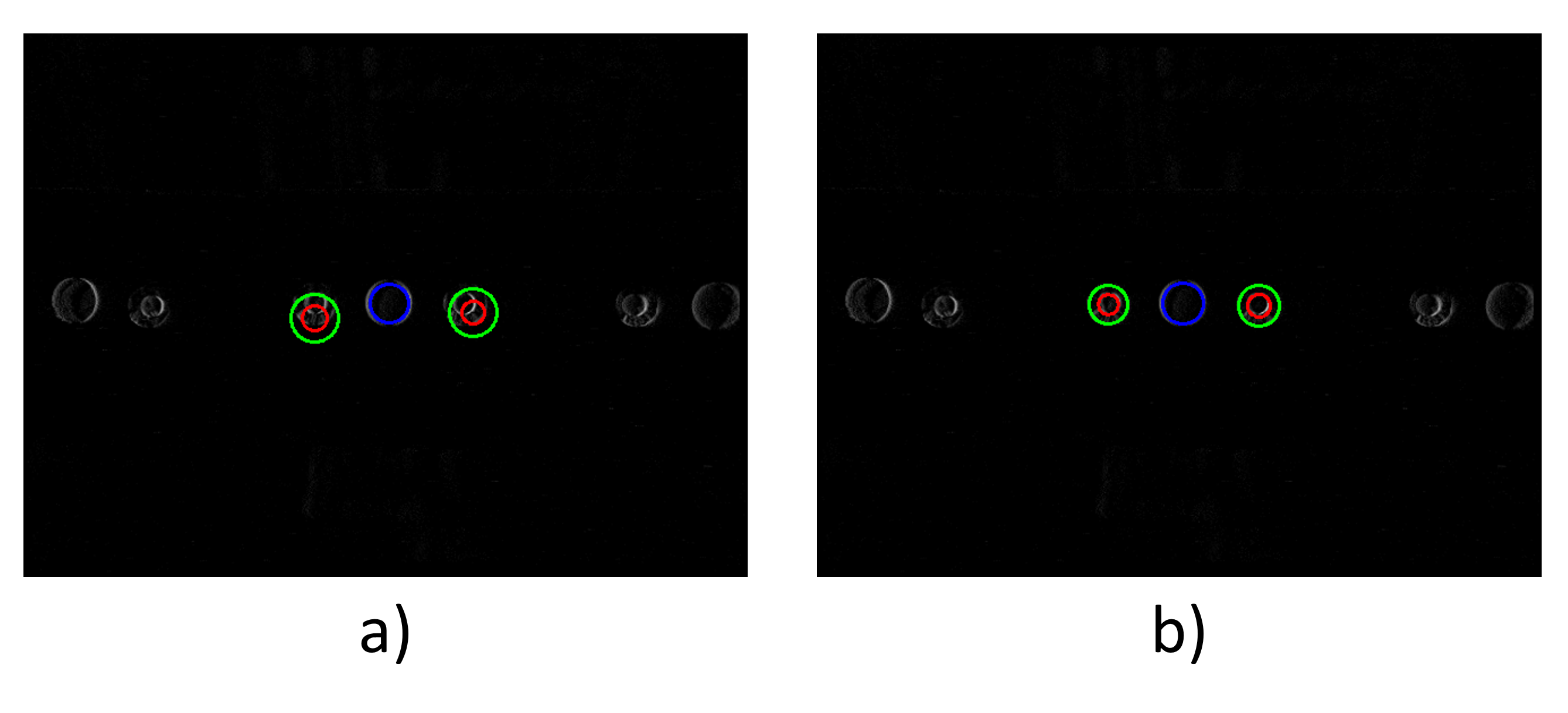
Figure 4: a) Circle fitting using ordinary least squares and b) robust fitting by Algorithm 1. The red and green circles represent the inner and outer edges of the. The blue circle is the pilot hole fitted using OLS.

Having the inner and outer radii, a known angle $\phi$, and $Z$, the depth $Z^{\prime}$ is estimated by simple trigonometry. Figure 5 presents front and isometric views of the s for a visual illustration of the trigonometric relation. First, the inner and outer radii are converted from pixels to mm by

$$\begin{bmatrix}r_{m}\\ R_{m}\end{bmatrix}=\begin{bmatrix}\frac{Z}{F}&0\\ 0&\frac{Z}{F}\end{bmatrix}\begin{bmatrix}r\\ R\end{bmatrix}$$ (19)

where $r_{m}$ and $R_{m}$ are the radii expressed in mm. Intuitively, $Z^{\prime}$ can be inferred from Figure 5 and is expressed by

$$Z^{\prime}=\frac{R_{m}-r_{m}}{\tan\frac{\phi}{2}}.$$ (20)

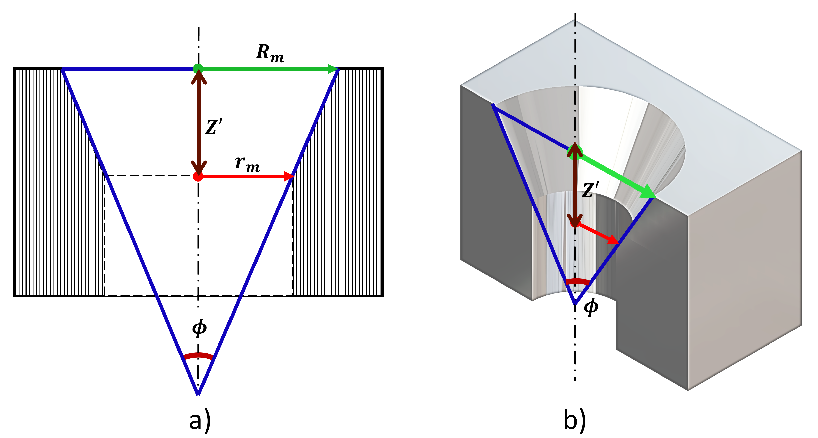
Figure 5: a) Front and b) isometric views of the. The depth $Z^{\prime}$ can be derived by trigonometry, given $r_{m}$, $R_{m}$, and $\phi$.

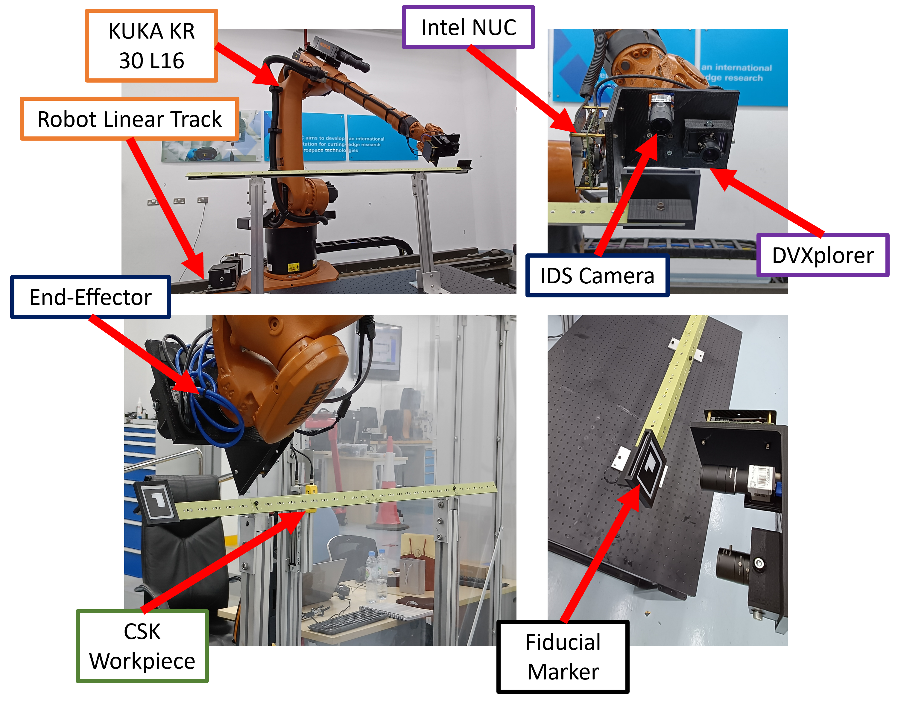
Figure 6: Experimental setup for validating the proposed inspection framework. A KUKA robotic manipulator is utilized for moving the neuromorphic camera to inspect a countersinks workpiece representing large industrial parts. A fiducial marker is installed on the workpiece for the normal alignment of the sensor with the workpiece.

4 Experimental Validation and Results

4.1 Experimental Setup

We have tested our framework in a variety of challenging scenarios. Fig. 6 shows the designed experimental setup to validate the proposed approach. A 7-DOF KUKA KR30 L16 with KL-1000-2 linear track was utilized to move the NVS during the inspection, and a workpiece resembling large indsutrial structures with inspection requirement. The robot end-effector comprises of IDS UI-5860CP ($1920\times 1080$) as the frame-based sensor for the normal alignment clarified in section 2.1, while the DVXplorer ($640\times 480$) as the NVS. Finally, Intel® NUC5i5RYH was also mounted on the end-effector for onboard processing, where both imaging sensors were interfaced with the robot operating system (ROS) using a USB 3.0 terminal. Four important aspects of the experimental protocol need to be taken into consideration. First, the NVS motion during the inspection ranged from 0.05 m/s to 0.5 m/s to justify the purpose of this paper. Second, the NVS moved in 2D linear motion as it sweeps the countersinks workpiece, as discussed in section 3.1. Third, we performed the proposed inspection method on three workpiece variants of different countersink sizes to show that the work of this paper is generalizable to different dimensions of countersink specimens, see Fig. 7. Finally, the standoff between the NVS and the workpiece during the sweep was $90mm$ to maintain high inspection precision. Videos of the experiments are available through the following link https://www.dropbox.com/s/pateqqwh4d605t3/final_video_new.mp4?dl=0.

The experimental validation of the proposed work revolves around three folds. In section 4.2, we compare the warping-Huber-based circle detection performance in terms of detection success rate and the IWEs image quality. We also compare the aforementioned detector to ED-Circles on frames from IDS camera and E2VID e2vid network for event-based image reconstruction. In section 4.3, we evaluate the precision and repeatability of the inspection by computing the standard deviation of the estimated depths on 10 runs at each NVS speed. Finally, section 4.4 benchmarks the work of this paper to state-of-the-art methods for inspection in terms of precision and inspection execution time.

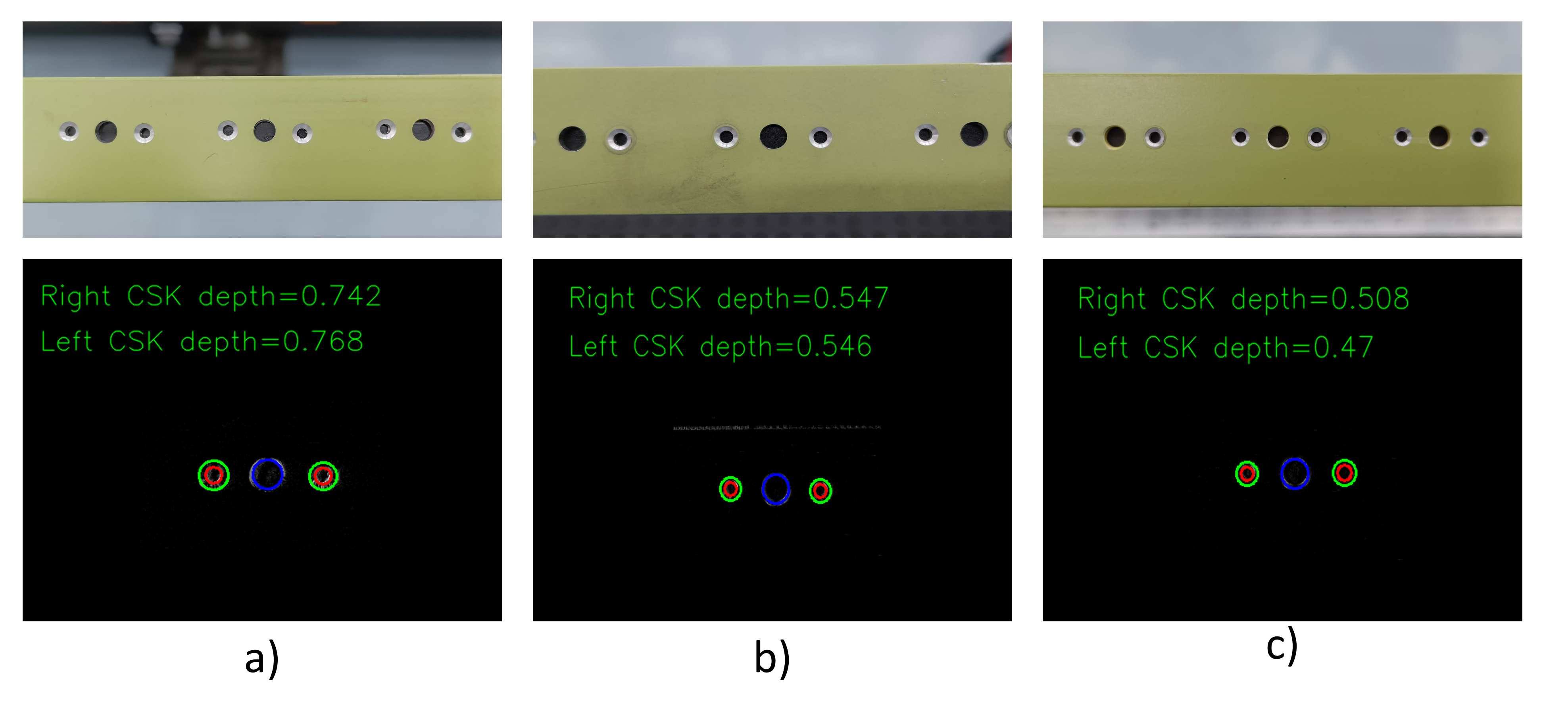
Figure 7: Inspected workpieces with countersinks of varying depth specifications along with the inspected specimens by our method. a)-c) are the workpiece IDs ordered in descending order with respect to the nominal countersink depths.

4.2 Countersink Detection Performance

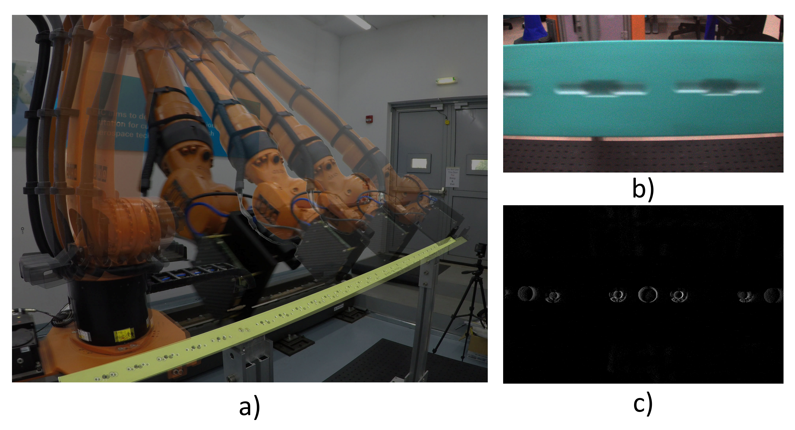
Figure 8: a) NVS motion trajectory during the inspection, b) and c) sharp IWEs and IDS frames suffering from motion blur. The reconstructed IWEs justify the purpose of the NVS for high-speed inspection.

	(a) Accumulated Event Frames $\Delta t=33ms$	(b) ED-Circles on IDS Frames	(c) ED-Circles on E2VID Reconstructed Images	(d) Proposed Detector
0.05 m/s NVS Speed
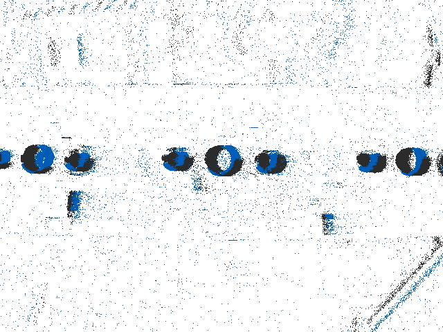
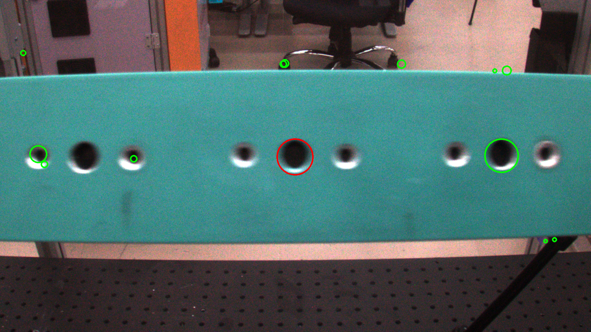
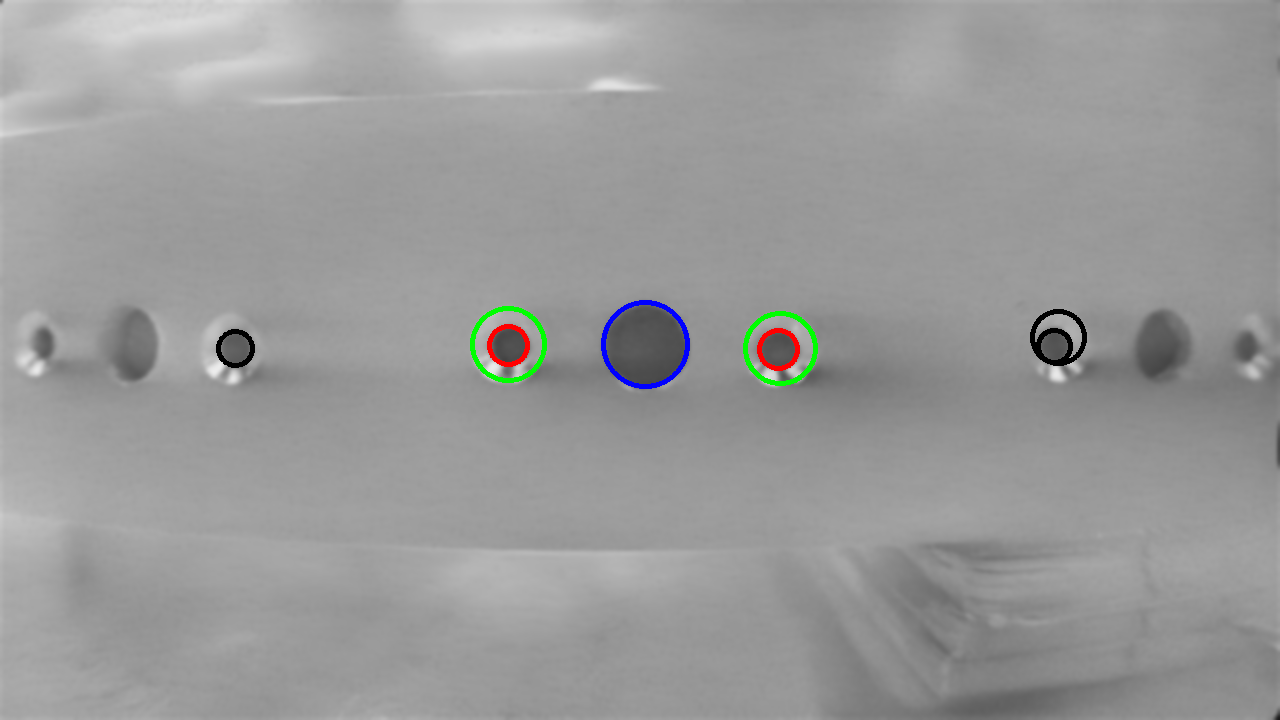
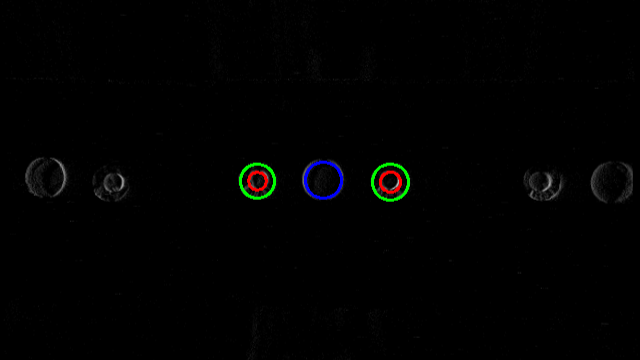
0.5 m/s NVS Speed

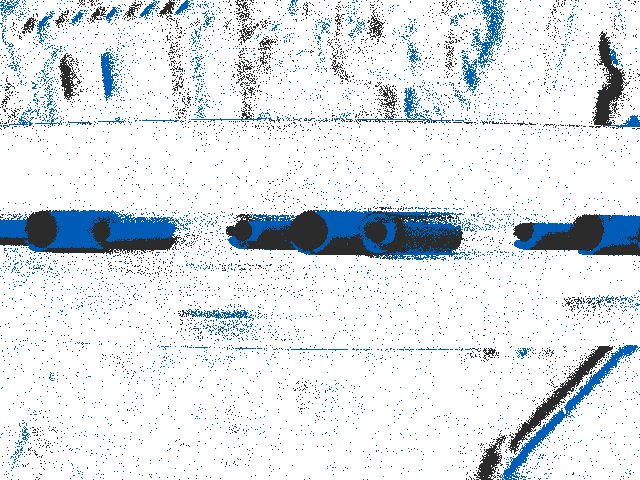
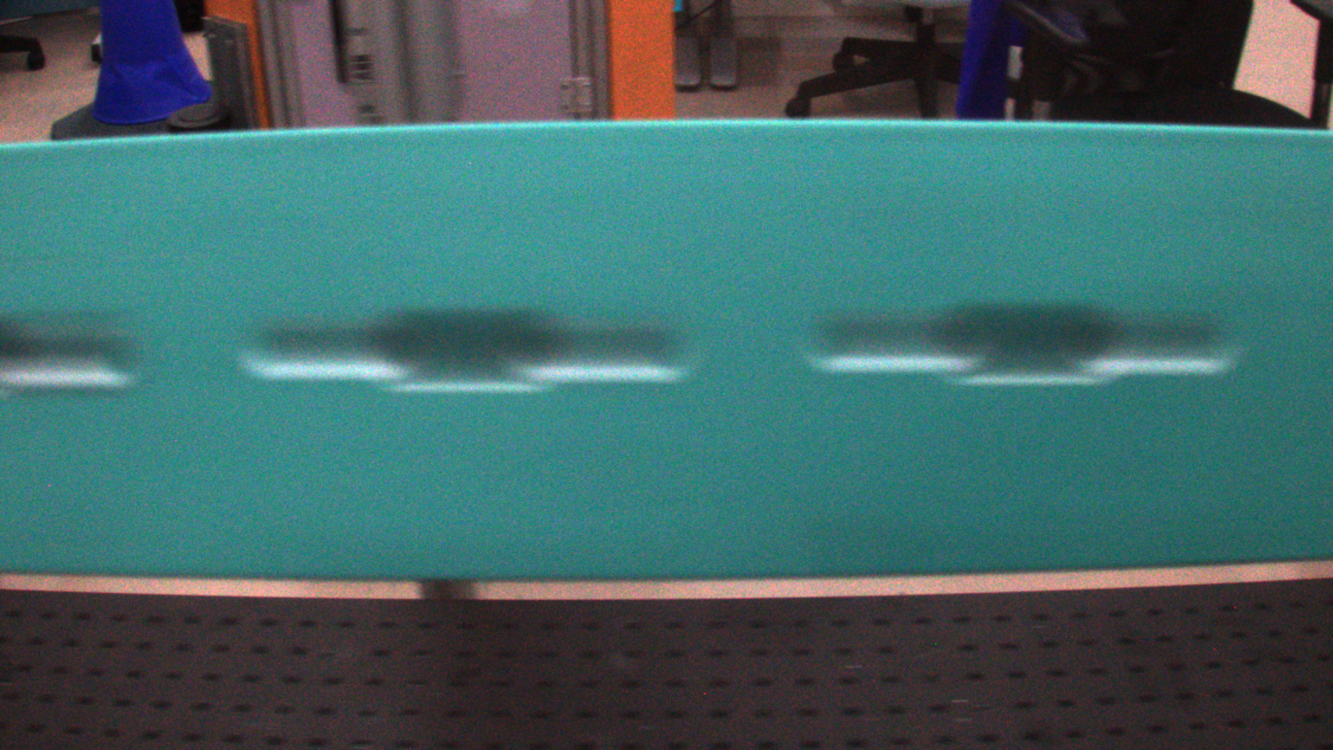
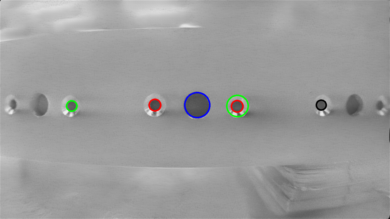
Figure 9: Qualitative comparison of the d) proposed detector with a) artificial event frames accumulated at $\Delta t=33ms$, b) conventional frames from the IDS camera, and c) E2VID reconstructed grayscale images. Notice that the features in the artificial event frames are perturbed by motion blur and noise, while features IDS images are degraded by motion blur even. On the other hand, E2VID provides textured image reconstruction of the scene, but ED-Circles fails due to reflections. Our detector, on the other hand, shows improved performance at high speeds with robustness against noise, reflection outliers, and motion blur.

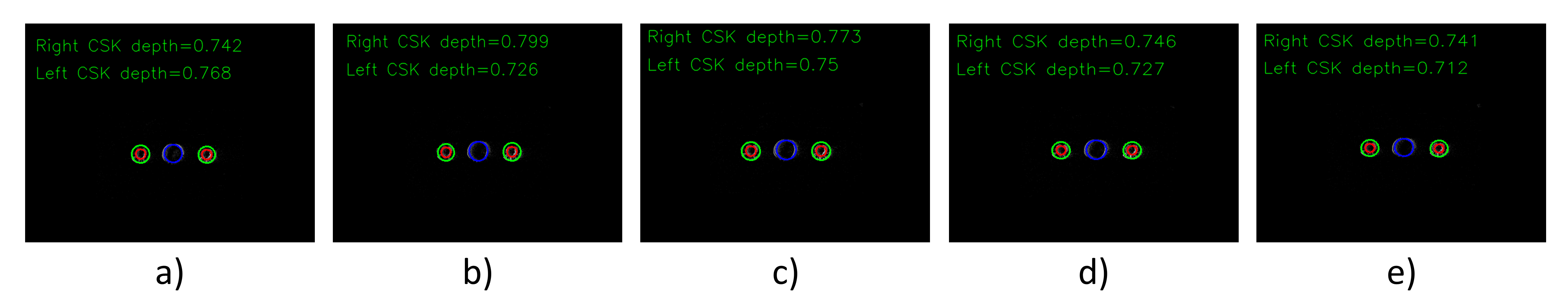
Figure 10: a)-e) Shows the precision of the proposed robust circle detection and depth estimation algorithms at 0.5 m/s. Notice the precise measurements even though the NVS resolution is relatively low.

The quality of the reconstructed IWEs directly impacts the detection performance. Figure 8 compares the obtained neuromorphic IWEs by warping against conventional images for a sweep speed of 0.5 m/s. If artificial event frames are formulated by simple accumulation at fixed time intervals, motion blur is witnessed, and the detection performance is highly influenced by sensor noise, see Figure 9. Given the improved quality of IWEs, the mean shift clustering algorithm for detection is evaluated based on its detection success rate, as a detection rate of 100% was obtained for speeds up to 0.5 m/s.

We also provide a qualitative comparison of the IWEs and the proposed circle detector in section 3.2 against ED-Circles applied on IDS conventional frames and reconstructed images from the E2VID e2vid network, illustrated in Figure 9. At 0.05 m/s, ED-Circles on IDS images fail to detect the circular edges of the countersinks due to motion blur, while detection was successful on E2VID network. This is because the network is characterized by its capability of reconstructing deblurred images of the scene. However, ED-Circles fail to detect the holes due to the inner wall reflections reducing the gradient of the circular edges at 0.5 m/s. In addition, E2VID requires a powerful GPU to run online, which is difficult to install on onboard processors. Contrary to the aforementioned approaches, the proposed detection pipeline runs on a low-end Intel® Core™ i5-5250U CPU, leverages the asynchronous nature of neuromorphic events, and demonstrates robustness against motion blur and outliers.

Table 1: Computation of standard deviation in mm for sample holes at a designated NVS speed for 10 trials. a)-c) represent the workpiece ID.

Hole ID	Trial Number										$\bm{\sigma_{d}}$
	1	2	3	4	5	6	7	8	9	10
1a	0.728	0.829	0.777	0.800	0.790	0.813	0.771	0.823	0.830	0.773	0.031
1b	0.557	0.574	0.570	0.544	0.511	0.526	0.545	0.532	0.584	0.534	0.025
1c	0.481	0.470	0.439	0.463	0.483	0.439	0.441	0.462	0.467	0.473	0.016

Table 2: Precision of the countersink inspection system in mm for 10 trials at each NVS speed for workpiece with ID ’A’, where a precision of 0.0275 mm is achieved.

Speed (m/s)	Hole ID
	1	2	3	4	5	6	7	8	9	10
0.05	0.021	0.020	0.028	0.022	0.031	0.029	0.035	0.017	0.011	0.029
0.1	0.016	0.023	0.011	0.023	0.034	0.035	0.033	0.036	0.032	0.035
0.2	0.022	0.018	0.016	0.025	0.028	0.031	0.026	0.025	0.029	0.028
0.3	0.023	0.016	0.021	0.029	0.033	0.026	0.021	0.033	0.032	0.029
0.5	0.031	0.031	0.030	0.033	0.027	0.032	0.025	0.019	0.033	0.026
$\sigma_{r}$	0.0209	0.022	0.0224	0.0267	0.0334	0.0307	0.0315	0.0271	0.0286	0.0296
									Aggregate	0.0275

Table 3: Precision of the countersink inspection system in mm for 10 trials at each NVS speed for workpiece with ID ’B’, where a precision of 0.0251 mm is achieved.

Speed (m/s)	Hole ID
	1	2	3	4	5	6	7	8	9	10
0.05	0.022	0.022	0.019	0.021	0.033	0.014	0.043	0.019	0.014	0.024
0.1	0.019	0.042	0.017	0.020	0.023	0.025	0.023	0.023	0.024	0.018
0.2	0.018	0.027	0.019	0.011	0.022	0.027	0.036	0.022	0.027	0.027
0.3	0.027	0.017	0.032	0.022	0.027	0.032	0.033	0.024	0.026	0.024
0.5	0.025	0.019	0.030	0.023	0.021	0.011	0.029	0.016	0.031	0.023
$\bm{\sigma_{r}}$	0.0261	0.0269	0.0242	0.0190	0.0256	0.0232	0.0335	0.0210	0.0251	0.0234
									Aggregate	0.0251

Table 4: Precision of the countersink inspection system in mm for 10 trials at each NVS speed for workpiece with ID ’C’, where a precision of 0.0240 mm is achieved.

Speed (m/s)	Hole ID
	1	2	3	4	5	6	7	8	9	10
0.05	0.017	0.024	0.033	0.024	0.024	0.027	0.021	0.020	0.034	0.019
0.1	0.026	0.018	0.021	0.019	0.012	0.029	0.018	0.019	0.016	0.021
0.2	0.023	0.022	0.016	0.013	0.017	0.030	0.016	0.027	0.026	0.027
0.3	0.013	0.011	0.027	0.011	0.019	0.023	0.034	0.029	0.027	0.027
0.5	0.016	0.012	0.019	0.021	0.020	0.021	0.032	0.037	0.028	0.029
$\bm{\sigma_{r}}$	0.0219	0.0182	0.0268	0.0183	0.0188	0.0262	0.0253	0.0272	0.0293	0.0249
									Aggregate	0.0240

4.3 Precision of Countersink Depth Estimation

While the proposed approach provides the required detection success rates, the precision of the depth estimation needs to be evaluated. The standard metric for evaluating the inspection is the standard deviation $\sigma_{d}$, where $\sigma_{d}$ was evaluated on each hole of each workpiece for 10 runs at distinct speeds of NVS. Table 1 shows the calculation $\sigma_{d}$ for a countersink sample from each workpiece at a speed of 0.5 m/s for 10 trials, and Figure 10 visualizes these estimations. The precision of the proposed inspection pipeline is directly correlated with the performance of the robust circle detection algorithm discussed in section 3.2. Notice that the radii of the fitted circles are consistent, where $\sigma_{d}$ = 0.031 mm was obtained. Tables 2, 3, 4 reports the precision of all $\sigma_{d}$ on each workpiece, where the proposed method provides an aggregate inspection precision of 0.025 mm.

Notice that the countersink inspection precision is higher for specimens with lower depths. This is because the motion compensation performance tends to be improved as the depth of the inner countersink walls is closer to the utilized depth for warping the events, as discussed in section 3.1. In all the cases however, the proposed inspection framework achieves a precision of 0.025 mm, abiding by the industrial requirements of various assembly lines. The reason behind the high precision of the proposed circle detector, even on a low-resolution sensor, is that it relies on an optimization approach fitting the best candidate circle to the observed hole edges. The high dependence of conventional circle detectors on the image gradient degrades their performance even on high-resolution cameras. Assuming that the conventional imaging sensor is static during the inspection and no motion blur is witnessed, the lighting conditions of the inspection setup have a major influence in controlling the precision of these circle detectors. In contrast, the high dynamic range of the NVS makes our method robust against illumination variations.

Table 5: Quantitative comparison of the proposed framework against state-of-the-art works for inspection using monocular vision. Even with a much lower resolution sensor, our method provides comparable results with the same order of magnitude against state-of-the-art approaches. Note that † indicates that the metric is unavailable.

Authors	Sensor Technology	Year	Sensor Resolution	Precision (mm)	Inspection Time (s)
R. Haldiman 3d_csk_measurement	DLP Projector	2015	†	0.03	†
Yu et al. yu2019vision	Conventional Camera	2019	2050 x 2448	0.02	42
Ours	NVS	2023	640 x 480	0.025	4.98

4.4 Benchmarks

To evaluate the impact of our event-driven approach, we compare the obtained results against state-of-the-art vision-based methods for inspection, which comprise of Haldiman’s 3d_csk_measurement inspection using Digital Light Processing (DLP) projector and Yu et al. work sa2018design . These works are compared quantitatively in terms of precision and qualitatively in terms of inspection speed, where the comparison is more elaborated in Table 5.

Our approach shows comparable results with the same orders of magnitude compared to previous works. The work of this paper outperforms Haldiman’ 3d_csk_measurement with the advantage of utilizing a neuromorphic sensor without the need for an active light projector. More importantly, the usage of laser projectors for depth estimation is currently unfavorable in industries for safety precautions, especially with the introduction of human-robot interaction in assembly lines. Yu et al. yu2019vision , on the other hand, outperforms our method by 0.0125 mm. Nevertheless, our method provides high-speed inspection and meets current industrial standards. Furthermore, the resolution of their utilized sensor is much higher than the DVXplorer by a factor of more than $1/16$. With the current advancements in neuromorphic sensor models, high-definition neuromorphic cameras easily circumvent this limitation and can provide improved precision.

In addition to high precision, our work provides the advantage of the swift execution time of the inspection task, with the capability of the NVS sweeping the workpiece at a high speed of 0.5 m/s. Table 6 reports the sweep time at different NVS speeds and illustrates that the 60 countersinks workpiece is scanned in nearly 3 seconds. Previous methods, in contrast, require the robot to pause on each countersink to perform the inspection before proceeding to the next hole. We quantify this by inspecting the holes using the IDS frames, and hole detection was carried out using ED-Circles and brute-force matching for outlier removal, in which these experiments mimic the works of Yu et al. yu2019vision . This is illustrated in Figure 11. During the inspection, the IDS camera paused on each hole for 0.5 seconds to carry on the inspection algorithm, and the motion between holes takes nearly 0.2 seconds. In total, the inspection task takes almost 42 seconds. One important aspect of our inspection pipeline is the computational time. Table 7 reports the total execution time for the proposed inspection pipeline algorithms. As 0.033 seconds are required to inspect each countersink, the total execution time of the neuromorphic vision-based inspection task is 4.98 seconds, reducing the inspection time by nearly a factor of 10. This also shows that the proposed work can be utilized to run online. It is worth mentioning that our algorithm was written in Python, and real-time capabilities can be achieved if written in C++.

Table 6: Sweep time at different NVS speeds for a 1.5 m countersinks workpiece.

Speed (m/s)	0.05	0.1	0.2	0.3	0.5
Sweep Time (s)	30	15	7.5	5	3

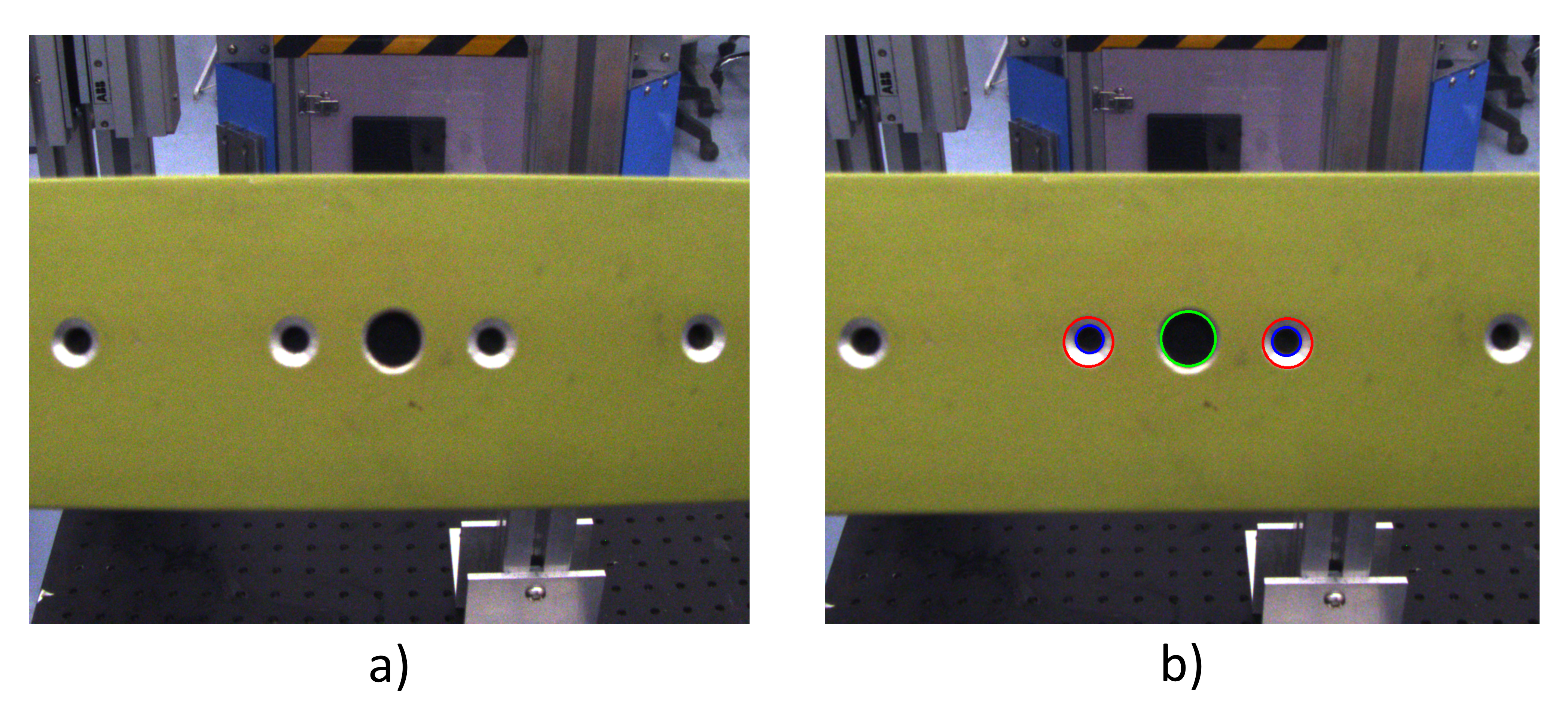
Figure 11: ED-Circles applied on a) IDS images. b) Reliable detection of countersinks requires the robot to pause at each hole due to high latency and motion blur.

Table 7: Execution times for the system blocks.

Algorithm	Execution Time (s)
Image of Warped Events Reconstruction	0.0084
Mean Shift Clustering	0.0178
Huber-Based Circle Fitting	0.007
Depth Estimation	0.000013
Total	0.0333

5 Conclusions and Future Work

In this paper, and for the first time, high-speed neuromorphic vision-based countersink inspection was proposed for automated assembly lines. The proposed approach leverages the neuromorphic vision sensor’s unprecedented asynchronous operation to create sharp, deblurred images through motion compensation. Due to the NVS unorthodox nature, a robust circle detection algorithm was devised to detect the countersinks in the IWEs. To prove the feasibility of neuromorphic vision for high-speed inspection, we have tested this paper’s work in various experiments for a low-resolution NVS reaching speeds up to 0.5 m/s. The high quality of the IWEs and the proposed circle detector played a major role in determining the precision of the proposed system. The experimental results show that over 60 countersinks can be inspected in less than 5 seconds while maintaining a precision of 0.025 mm. For future work, we aim to develop an event-based fiducial marker detection algorithm to utilize the NVS solely for the whole inspection procedure, starting from the initial alignment of the sensor with the inspected workpiece to its high-speed sweep. On the other hand, while the introduced motion compensation-circle detection frameworks were utilized for inspection, these algorithms will be further deployed for robotic positioning systems and visual servoing in automated manufacturing processes such as precision drilling, deburring, and various other robotic manufacturing opportunities.

Author Contribution

Mohammed Salah Conceptualization, Methodology, Software, Investigation, Data collection, Experimentation, Writing. Abdulla Ayyad Conceptualization, Methodology, Software, Investigation, Data collection, Experimentation, Writing. Mohammed Ramadan End-effector Design, Software, Writing. Yusra Abdulrahman Technical Advising, Writing. Dewald Swart Conceptualization, Software. Abdelqader Abusafieh Methodology, Technical Advising. Lakmal Seneviratne Supervision, Funding acquisition, Technical Advising. Yahya Zweiri Project management, Funding acquisition, Review and Editing.

Conflict of interest

The authors declare that they have no conflict of interest.

References

- [1] Ali Karim and Alexander Verl. Challenges and obstacles in robot-machining. In IEEE ISR 2013, pages 1–4. IEEE, 2013.
- [2] Deepesh Jayasekara, Nai Yeen Gavin Lai, Kok-Hoong Wong, Kulwant Pawar, and Yingdan Zhu. Level of automation (loa) in aerospace composite manufacturing: Present status and future directions towards industry 4.0. Journal of Manufacturing Systems, 62:44–61, 2022.
- [3] Robert U. Ayres and Jeffrey L. Funk. The role of machine sensing in cim. Robotics and Computer-Integrated Manufacturing, 5(1):53–71, 1989.
- [4] Te-Hsiu Sun, Fang-Cheng Tien, Fang-Chih Tien, and Ren-Jieh Kuo. Automated thermal fuse inspection using machine vision and artificial neural networks. Journal of Intelligent Manufacturing, 27, 03 2014.
- [5] Yuri DV Yasuda, Fabio AM Cappabianco, Luiz Eduardo G Martins, and Jorge AB Gripp. Aircraft visual inspection: A systematic literature review. Computers in Industry, 141:103695, 2022.
- [6] Kleber Roberto da Silva Santos, Wesley Rodrigues de Oliveira, Emília Villani, and Augusto Dttmann. 3d scanning method for robotized inspection of industrial sealed parts. Computers in Industry, 147:103850, 2023.
- [7] Lubna Shahid, Farrokh Janabi-Sharifi, and Patrick Keenan. A hybrid vision-based surface coverage measurement method for robotic inspection. Robotics and Computer-Integrated Manufacturing, 57:138–145, 2019.
- [8] Ssu-Han Chen and Der-Baau Perng. Automatic optical inspection system for ic molding surface. Journal of Intelligent Manufacturing, 27, 06 2014.
- [9] Tatyana Kruglova, Daher Sayfeddine, and Kovalenko Vitaliy. Robotic laser inspection of airplane wings using quadrotor. Procedia engineering, 129:245–251, 2015.
- [10] Jiming Sa, Feng Ye, Yue Shao, Yilun An, and Shaogang Wan. Design and realization of counterbore inspection system based on machine vision. In 2018 5th International Conference on Systems and Informatics (ICSAI), pages 87–92. IEEE, 2018.
- [11] R. Haldiman. 3d countersink measurement, 2015.
- [12] Nguyen Duy Minh Phan, Yann Quinsat, Sylvain Lavernhe, and Claire Lartigue. Path planning of a laser-scanner with the control of overlap for 3d part inspection. Procedia Cirp, 67:392–397, 2018.
- [13] Andrzej Burghardt, Krzysztof Kurc, Dariusz Szybicki, Magdalena Muszyńska, and Tomasz Szczęch. Robot-operated inspection of aircraft engine turbine rotor guide vane segment geometry. Technical Gazette, 24(2):345–348, 2017.
- [14] Habiba Zahir Imam, Hamdan Al-Musaibeli, Yufan Zheng, Pablo Martinez, and Rafiq Ahmad. Vision-based spatial damage localization method for autonomous robotic laser cladding repair processes. Robotics and Computer-Integrated Manufacturing, 80:102452, 2023.
- [15] Joshua Smith and Duncan Kochhar-Lindgren. Integrated hole and countersink inspection of aircraft components, 2013.
- [16] Zachary Luker and Erin Stansbury. In-process hole and fastener inspection using a high-accuracy laser sensor. SAE Technical Paper, 2(2020-01-0015), 2020.
- [17] Long Yu, Qingzhen Bi, Yulei Ji, Yunfei Fan, Nuodi Huang, and Yuhan Wang. Vision based in-process inspection for countersink in automated drilling and riveting. Precision Engineering, 58:35–46, 2019.
- [18] Walter Nsengiyumva, Shuncong Zhong, Jiewen Lin, Qiukun Zhang, Jianfeng Zhong, and Yuexin Huang. Advances, limitations and prospects of nondestructive testing and evaluation of thick composites and sandwich structures: A state-of-the-art review. Composite Structures, 256:112951, 2021.
- [19] James H Wang and Michael R Wang. Handheld non-contact evaluation of fastener flushness and countersink surface profiles using optical coherence tomography. Optics Communications, 371:206–212, 2016.
- [20] Yusra Alkendi, Rana Azzam, Abdulla Ayyad, Sajid Javed, Lakmal Seneviratne, and Yahya Zweiri. Neuromorphic camera denoising using graph neural network-driven transformers, 2021.
- [21] Christian Brandli, Raphael Berner, Minhao Yang, Shih-Chii Liu, and Tobi Delbruck. A 240 × 180 130 db 3 µs latency global shutter spatiotemporal vision sensor. IEEE Journal of Solid-State Circuits, 49(10):2333–2341, 2014.
- [22] Guillermo Gallego, Tobi Delbrück, Garrick Orchard, Chiara Bartolozzi, Brian Taba, Andrea Censi, Stefan Leutenegger, Andrew J. Davison, Jörg Conradt, Kostas Daniilidis, and Davide Scaramuzza. Event-based vision: A survey. IEEE Transactions on Pattern Analysis and Machine Intelligence, 44(1):154–180, 2022.
- [23] Mohammed Salah, Mohammed Chehadah, Muhammad Humais, Mohammed Wahbah, Abdulla Ayyad, Rana Azzam, Lakmal Seneviratne, and Yahya Zweiri. A neuromorphic vision-based measurement for robust relative localization in future space exploration missions. IEEE Transactions on Instrumentation and Measurement, pages 1–1, 2022.
- [24] Florian Mahlknecht, Daniel Gehrig, Jeremy Nash, Friedrich M. Rockenbauer, Benjamin Morrell, Jeff Delaune, and Davide Scaramuzza. Exploring event camera-based odometry for planetary robots, 2022.
- [25] Peter N. McMahon-Crabtree and David G. Monet. Commercial-off-the-shelf event-based cameras for space surveillance applications. Appl. Opt., 60(25):G144–G153, Sep 2021.
- [26] Abdulla Ayyad, Mohamad Halwani, Dewald Swart, Rajkumar Muthusamy, Fahad Almaskari, and Yahya Zweiri. Neuromorphic vision based control for the precise positioning of robotic drilling systems. Robotics and Computer-Integrated Manufacturing, 79:102419, 2023.
- [27] Bin Li, Hu Cao, Zhongnan Qu, Yingbai Hu, Zhenke Wang, and Zichen Liang. Event-based robotic grasping detection with neuromorphic vision sensor and event-grasping dataset. Frontiers in Neurorobotics, 14, 2020.
- [28] Xiaoqian Huang, Mohamad Halwani, Rajkumar Muthusamy, Abdulla Ayyad, Dewald Swart, Lakmal Seneviratne, Dongming Gan, and Yahya Zweiri. Real-time grasping strategies using event camera. Journal of Intelligent Manufacturing, 33, 02 2022.
- [29] Johan Bertrand, Arda Yiğit, and Sylvain Durand. Embedded event-based visual odometry. In 2020 6th International Conference on Event-Based Control, Communication, and Signal Processing (EBCCSP), pages 1–8, 2020.
- [30] Daqi Liu, Alvaro Parra, and Tat-Jun Chin. Spatiotemporal registration for event-based visual odometry, 2021.
- [31] Fariborz Baghaei Naeini, Aamna M. AlAli, Raghad Al-Husari, Amin Rigi, Mohammad K. Al-Sharman, Dimitrios Makris, and Yahya Zweiri. A novel dynamic-vision-based approach for tactile sensing applications. IEEE Transactions on Instrumentation and Measurement, 69(5):1881–1893, 2020.
- [32] Amin Rigi, Fariborz Baghaei Naeini, Dimitrios Makris, and Yahya Zweiri. A novel event-based incipient slip detection using dynamic active-pixel vision sensor (davis). Sensors, 18(2), 2018.
- [33] Oussama Abdul Hay, Mohamad Chehadeh, Abdulla Ayyad, Mohamad Wahbah, Muhammad Humais, and Y Zweiri. Unified identification and tuning approach using deep neural networks for visual servoing applications. arXiv preprint arXiv:2107.01581, 2021.
- [34] Abdulla Ayyad, Mohamad Halwani, Dewald Swart, Rajkumar Muthusamy, Fahad Almaskari, and Yahya Zweiri. Neuromorphic vision based control for the precise positioning of robotic drilling systems. Robotics and Computer-Integrated Manufacturing, 79:102419, 2023.
- [35] Francisco J. Romero-Ramirez, Rafael Muñoz-Salinas, and Rafael Medina-Carnicer. Speeded up detection of squared fiducial markers. Image and Vision Computing, 76:38–47, 2018.
- [36] Mohamad Halwani, Abdulla Ayyad, Laith AbuAssi, Yusra Abdulrahman, Fahad Almaskari, Hany Hassanin, Abdulqader Abusafieh, and Yahya Zweiri. A novel vision-based multi-functional sensor for normality and position measurements in precise robotic manufacturing. SSRN Electronic Journal, 01 2023.
- [37] Guillermo Gallego, Henri Rebecq, and Davide Scaramuzza. A unifying contrast maximization framework for event cameras, with applications to motion, depth, and optical flow estimation. Proceedings / CVPR, IEEE Computer Society Conference on Computer Vision and Pattern Recognition. IEEE Computer Society Conference on Computer Vision and Pattern Recognition, 06 2018.
- [38] Timo Stoffregen, Guillermo Gallego, Tom Drummond, Lindsay Kleeman, and Davide Scaramuzza. Event-based motion segmentation by motion compensation. In 2019 IEEE/CVF International Conference on Computer Vision (ICCV). IEEE, oct 2019.
- [39] Bruno Siciliano and Oussama Khatib. Springer Handbook of Robotics. Springer-Verlag, Berlin, Heidelberg, 2007.
- [40] K Sreedhar. Enhancement of images using morphological transformations. International Journal of Computer Science and Information Technology, 4(1):33–50, feb 2012.
- [41] D. Comaniciu and P. Meer. Mean shift: a robust approach toward feature space analysis. IEEE Transactions on Pattern Analysis and Machine Intelligence, 24(5):603–619, 2002.
- [42] Cihan Topal, Ozgur Ozsen, and Cuneyt Akinlar. Real-time edge segment detection with edge drawing algorithm. In 2011 7th International Symposium on Image and Signal Processing and Analysis (ISPA), pages 313–318, 2011.
- [43] Cuneyt Akinlar and Cihan Tonal. Edcircles: Real-time circle detection by edge drawing (ed). In 2012 IEEE International Conference on Acoustics, Speech and Signal Processing (ICASSP), pages 1309–1312, 2012.
- [44] Peter J. Huber. Robust estimation of a location parameter. The Annals of Mathematical Statistics, 35(1):73–101, 1964.
- [45] KENNETH LEVENBERG. A method for the solution of certain non-linear problems in least squares. Quarterly of Applied Mathematics, 2(2):164–168, 1944.
- [46] Henri Rebecq, René Ranftl, Vladlen Koltun, and Davide Scaramuzza. High speed and high dynamic range video with an event camera. IEEE Trans. Pattern Anal. Mach. Intell. (T-PAMI), 2019.