A comparison of Krylov methods
for Shifted Skew-Symmetric Systems

Abstract

It is well known that for general linear systems, only optimal Krylov methods with long recurrences exist. For special classes of linear systems it is possible to find optimal Krylov methods with short recurrences. In this paper we consider the important class of linear systems with a shifted skew-symmetric coefficient matrix. We present the MRS³ solver, a minimal residual method that solves these problems using short vector recurrences. We give an overview of existing Krylov solvers that can be used to solve these problems, and compare them with the MRS³ method, both theoretically and by numerical experiments. From this comparison we argue that the MRS³ solver is the fastest and most robust of these Krylov method for systems with a shifted skew-symmetric coefficient matrix.

Keywords: Lanczos, Krylov, Minimal Residual, Short Recurrences, Shifted Skew-Symmetric
AMS Subject Classification: 65F10

1 Introduction

In this paper we explore Krylov subspace methods that can solve systems of linear equations of the form

$$A\mathbf{x}=\mathbf{b},$$ (1)

where $A\in\mathbb{R}^{n\times n}$ is a shifted skew-symmetric matrix, i.e.,

$$A=\alpha I+S,~{}\alpha\in\mathbb{R},~{}S^{T}=-S.$$ (2)

Throughout this paper we will use $I$ for the identity matrix of appropriate size, $H$ for symmetric matrices, and $S$ for skew-symmetric matrices as above. Further we will use the abbreviation SSS for shifted skew-symmetric. Note that SSS matrices are normal, i.e., $AA^{T}=A^{T}A$.

Our research on this problem was previously available as a technical report [18]. Due to the increasing interest in shifted skew-symmetric problems, we decided to now formally publish the work.

Shifted skew-symmetric systems arise in many scientific and engineering applications, like computational fluid dynamics, linear programming and systems theory.

In computational fluid dynamics, SSS systems arise when dealing with Navier-Stokes equations with a large [10] or a small [11] Reynolds number (see also [2]).

Consider $B$ to be a large nonsingular matrix, which is a discrete version of an advection-diffusion problem. The Hermitian splitting can be used to decompose $B$ in its symmetric part $H$ and its skew-symmetric part $S$:

$$B=H+S,\textrm{ where }H=\frac{B+B^{T}}{2}\textrm{ and }S=\frac{B-B^{T}}{2}.$$

If the diffusion is important, i.e., if the Reynolds number is small, and if the symmetric part $H$ of $B$ is positive definite, $H^{-1}$ can be used as a preconditioner to solve a system $B\mathbf{x}=\mathbf{b}$. Note that to compute $\mathbf{v}=H^{-1}\mathbf{w}$ efficiently, multigrid can be used. The preconditioning can be done as follows:

$$H^{-\frac{1}{2}}BH^{-\frac{1}{2}}\mathbf{y}=H^{-\frac{1}{2}}\mathbf{b},\textrm{ where }\mathbf{x}=H^{-\frac{1}{2}}\mathbf{y}.$$ (3)

This equation can then be rewritten as

$$(I+H^{-\frac{1}{2}}SH^{-\frac{1}{2}})\mathbf{y}=H^{-\frac{1}{2}}\mathbf{b},$$

which is an SSS system (compare [11]).

On the other hand if advection is dominant, i.e., if the Reynolds number is large,

$$\left(I-(\alpha I+S)^{-1}(H-\alpha I)\right)(\alpha I+S)^{-1}$$

can be used as a preconditioner (see [10] eq. (1.7) and (3.1)). Applying this preconditioner to a vector $\mathbf{w}$ implies that SSS systems of the form $(\alpha I+S)\mathbf{v}=\mathbf{w}$ have to be solved.

For an application in linear programming consider interior point methods, a popular way of solving linear programming problems. When solving a linear program with such a method, using a self-dual embedding of the problem takes slightly more computational time per iteration but has several important advantages such as having a centered starting point and detecting infeasibility by convergence, as described in [24]. Therefore, most modern solvers use such an embedding.

Interior point methods are iterative schemes that search for an optimal solution from within the strictly feasible set. In each iteration a step $\Delta\mathbf{x}_{i}$ to add to the current solution is generated. To calculate this step, a large sparse system has to be solved, that is of the form

$$(D_{i}+S)\Delta\mathbf{x}_{i}=\mathbf{b}_{i},$$ (4)

where $S$ is a skew-symmetric matrix and $D_{i}$ is a diagonal matrix with strictly positive diagonal entries. Using the same preconditioning as in equation (3), we can rewrite system (4) as

$$(I+D_{i}^{-\frac{1}{2}}SD_{i}^{-\frac{1}{2}})\mathbf{y}_{i}=D_{i}^{-\frac{1}{2}}\mathbf{b}_{i},\textrm{ where }\mathbf{y}_{i}=D_{i}^{\frac{1}{2}}\Delta\mathbf{x}_{i}\,.$$ (5)

This again is an SSS system. Note that the preconditioning used is in fact diagonal scaling.

In systems theory, shifted skew-symmetric linear systems arise in the discretization of port-Hamiltonian problems [20].

In this paper, we aspire to give an overview of Krylov methods available to solve Shifted Skew-Symmetric systems, and we present MRS³, a Minimal Residual method for SSS systems, designed specifically for solving such systems. In Section 2 we review existing methods, and their application to SSS systems. The MRS³ algorithm is presented in Section 3. In Section 4 we do a theoretical comparison of the treated methods, followed in Section 5 by the results of our numerical experiments. Finally, in Section 6 we present our conclusions with respect to solvers for SSS systems.

2 Overview of existing methods

In this section we give an overview of some existing Krylov subspace methods, that can be used to solve shifted skew-symmetric systems. In iteration $j$, a Krylov subspace method approximates the solution with $\mathbf{x}_{j}=\mathbf{x}_{0}+\mathbf{s}_{j}$, where $\mathbf{s}_{j}\in\mathcal{K}_{j}(A,\mathbf{r}_{0})$. Here $\mathbf{x}_{0}$ is the initial solution, $A$ is the coefficient matrix of the system, $\mathbf{r}_{0}=\mathbf{b}-A\mathbf{x}_{0}$ is the initial residual, and $\mathcal{K}_{j}(A,\mathbf{r}_{0})$ is the Krylov subspace:

$$\mathcal{K}_{j}(A,\mathbf{r}_{0})=\textrm{span}\{\mathbf{r}_{0},A\mathbf{r}_{0},\ldots,A^{j-1}\mathbf{r}_{0}\}.$$

Since in every iteration the Krylov subspace is expanded, a new approximation within the larger subspace can be generated that is never worse than the previous one.

Two important properties of Krylov subspace methods are optimality and short recurrences. An algorithm has the optimality property if the generated approximation for the solution is, measured in some norm, the best within the current Krylov subspace. The short recurrences property is satisfied if the algorithm can generate the next approximation using only data from the last few iterations.

For general coefficient matrices the above properties cannot be attained simultaneously. However methods satisfying both properties do exist for matrices of the form

$$A=e^{i\theta}(\sigma I+T)\textrm{, where }\theta\in\mathbb{R},~{}\sigma\in\mathbb{C},~{}T^{H}=T.$$

These results are due to Voevodin [32] and Faber and Manteuffel [8], [9]. Taking $\theta=\pi/2$, $\sigma=-i\alpha$ with $\alpha\in\mathbb{R}$ and $T=-iS$ with $S^{T}=-S$, we get an SSS matrix as given in equation (2). This implies that a Krylov subspace method for SSS systems exists, that has both the optimality property and short recurrences.

2.1 General methods

An SSS system can be solved with any solver for general systems of linear equations. We will treat a few widely used methods, that nicely illustrate the findings of Voevodin and Faber and Manteuffel mentioned above.

GMRES [26] generates optimal approximations to the solution, but needs vectors from all the previous iterations to do so. For more details see the remarks about GMRES at the start of Section 4.

GCR [7], [30] also generates optimal approximations, and generally needs vectors from all previous iterations. However for SSS systems, the orthogonalization can be done with information from the last iteration only. Truncating the orthogonalization of GCR is commonly known as Truncated GCR, or Orthomin($k$) [31]. So, in other words, for SSS systems Orthomin(1) is the same as full GCR, as is shown in Theorem 2.2. However, there are examples where GCR breaks down, whereas GMRES does not. For details see Section 2.2 below.

Bi-CGSTAB [28] uses short recurrences but does not have the optimality property. Usually it converges fast but it is not very robust.

Finally, CGNR [23] solves the normal equations $A^{T}A\mathbf{x}=A^{T}\mathbf{b}$ with the CG method. This solver achieves both optimality and short recurrences, but in a different Krylov subspace, namely $\mathcal{K}_{j}(A^{T}A,A^{T}\mathbf{r}_{0})$. Since the condition number is squared when working with $A^{T}A$, convergence can be very slow for ill-conditioned systems. This method is used for solving SSS systems by Golub and Vanderstraeten in their treatment of the preconditioning of matrices with a large skew-symmetric part [10]. For a regularization technique using CGNR, designed specifically to deal with very ill-conditioned skew-symmetric systems, we refer to [3].

2.2 Truncated GCR

Below we present the GCR algorithm, truncated after one orthogonalization step, also known as Orthomin(1).

Algorithm 2.1 (Truncated GCR).

• Let $\mathbf{x}_{0}$ be given, $\mathbf{r}_{0}=\mathbf{b}-A\mathbf{x}_{0}$, $\mathbf{v}_{0}=\mathbf{0}$, $j=0$

• While not converged do

  • $j=j+1$

  • $\mathbf{s}_{j}=\mathbf{r}_{j-1}$ and $\mathbf{v}_{j}=A\mathbf{r}_{j-1}$

  • $\mu_{j}=\left(\mathbf{v}_{j-1},\mathbf{v}_{j}\right)$

  • $\mathbf{s}_{j}=\mathbf{s}_{j}-\mu_{j}\mathbf{s}_{j-1}$ and $\mathbf{v}_{j}=\mathbf{v}_{j}-\mu_{j}\mathbf{v}_{j-1}$

  • $\beta_{j}=\left|\left|\mathbf{v}_{j}\right|\right|_{2}$

  • $\mathbf{s}_{j}=\mathbf{s}_{j}/\beta_{j}$ and $\mathbf{v}_{j}=\mathbf{v}_{j}/\beta_{j}$

  • $\gamma_{j}=\left(\mathbf{r}_{j-1},\mathbf{v}_{j}\right)$

  • $\mathbf{x}_{j}=\mathbf{x}_{j-1}+\gamma_{j}\mathbf{s}_{j}$ and $\mathbf{r}_{j}=\mathbf{r}_{j-1}-\gamma_{j}\mathbf{v}_{j}$

• Endwhile

The full GCR algorithm is the same, except that the orthogonalization step reads

$$\mathbf{s}_{j}=\mathbf{s}_{j}-\sum_{i=1}^{j-1}\left(\mathbf{v}_{i},\mathbf{v}_{j}\right)\mathbf{s}_{i}\textrm{~{}~{}and~{}~{}}\mathbf{v}_{j}=\mathbf{v}_{j}-\sum_{i=1}^{j-1}\left(\mathbf{v}_{i},\mathbf{v}_{j}\right)\mathbf{v}_{i}.$$ (6)

Thus the value of $\mathbf{v}_{j}$ at the end of each iteration is $\mathbf{v}_{j}=\frac{1}{\beta_{j}}\left(A\mathbf{r}_{j-1}-\sum_{i=1}^{j-1}\left(\mathbf{v}_{i},A\mathbf{r}_{j-1}\right)\mathbf{v}_{i}\right)$, for full GCR. We will use $\beta_{j}\mathbf{v}_{j}$ to denote the value of $\mathbf{v}_{j}$ just before the normalization step.

First note that in full GCR $\mathbf{v}_{j}\perp\mathbf{v}_{1},\ldots,\mathbf{v}_{j-1}$ by construction, thus

$$\left(\mathbf{v}_{j},\mathbf{v}_{i}\right)=0,\textrm{ for all }i<j.$$ (7)

Further note that

$$\left(\mathbf{r}_{j},\mathbf{v}_{i}\right)=0,\textrm{ for all }i\leq j,$$ (8)

because we have $\left(\mathbf{r}_{j},\mathbf{v}_{j}\right)=\left(\mathbf{r}_{j-1}-\gamma_{j}\mathbf{v}_{j},\mathbf{v}_{j}\right)=\left(\mathbf{r}_{j-1},\mathbf{v}_{j}\right)-\gamma_{j}\left(\mathbf{v}_{j},\mathbf{v}_{j}\right)=\gamma_{j}-\gamma_{j}=0$, and for $i<j$ we find $\left(\mathbf{r}_{j},\mathbf{v}_{i}\right)=\left(\mathbf{r}_{i}-\sum_{k=i+1}^{j}\gamma_{k}\mathbf{v}_{k},\mathbf{v}_{i}\right)=\left(\mathbf{r}_{i},\mathbf{v}_{i}\right)-\sum_{k=i+1}^{j}\gamma_{k}\left(\mathbf{v}_{k},\mathbf{v}_{i}\right)=0.$

Below we will present a few properties of non-truncated GCR, that are often regarded common knowledge in the linear algebra community, but that we have not been able to find references to their explicit proofs for. For completeness we have therefore included proofs ourselves.

Lemma 2.1.

In GCR, if $\gamma_{j}=0$ for some $j$, the algorithm breaks down in iteration $j+1$.

Proof.

If $\gamma_{j}=0$ then $\mathbf{r}_{j}=\mathbf{r}_{j-1}$. Therefore we can write

$$\beta_{j+1}\mathbf{v}_{j+1}=A\mathbf{r}_{j}-\sum_{i=1}^{j}\left(\mathbf{v}_{i},A\mathbf{r}_{j}\right)\mathbf{v}_{i}\\ =A\mathbf{r}_{j-1}-\sum_{i=1}^{j-1}\left(\mathbf{v}_{i},A\mathbf{r}_{j-1}\right)\mathbf{v}_{i}-\left(\mathbf{v}_{j},A\mathbf{r}_{j-1}\right)\mathbf{v}_{j}.$$

The first two terms of the right hand side together are equal to $\beta_{j}\mathbf{v}_{j}$, whereas the last term we can rewrite using that $A\mathbf{r}_{j-1}=\beta_{j}\mathbf{v}_{j}+\sum_{i=1}^{j-1}\left(\mathbf{v}_{i},A\mathbf{r}_{j-1}\right)\mathbf{v}_{i}$, and the orthogonality relation (7):

$$\left(\mathbf{v}_{j},A\mathbf{r}_{j-1}\right)\mathbf{v}_{j}=\left(\mathbf{v}_{j},\beta_{j}\mathbf{v}_{j}+\sum_{i=1}^{j-1}\left(\mathbf{v}_{i},A\mathbf{r}_{j-1}\right)\mathbf{v}_{i}\right)\mathbf{v}_{j}=\beta_{j}\left(\mathbf{v}_{j},\mathbf{v}_{j}\right)\mathbf{v}_{j}=\beta_{j}\mathbf{v}_{j}.$$

Thus we find that $\beta_{j+1}\mathbf{v}_{j+1}=\beta_{j}\mathbf{v}_{j}-\beta_{j}\mathbf{v}_{j}=0$. Then the normalization factor $\beta_{j+1}=0$, and the algorithm breaks down on the calculation of $\mathbf{v}_{j+1}=\frac{\mathbf{0}}{0}$. ∎

Theorem 2.1.

When GCR is applied to a system with skew-symmetric coefficient matrix $S$, the algorithm breaks down in the second iteration.

Proof.

Using that $\mathbf{z}^{T}S\mathbf{z}=0$ for any vector $\mathbf{z}$, we find $\gamma_{1}=\left(\mathbf{r}_{0},\mathbf{v}_{1}\right)=\left(\mathbf{r}_{0},\frac{1}{\beta_{1}}S\mathbf{r}_{0}\right)=0$. Thus the statement follows readily from Lemma 2.1. ∎

As mentioned before, for SSS systems Algorithm 2.1 gives the same iterates as full GCR. The following theorem proves this fact, by showing that the coefficients of all those orthogonalization factors that are omitted in Algorithm 2.1, are equal to 0 for SSS systems.

Theorem 2.2.

When GCR is applied to a system with shifted skew-symmetric coefficient matrix $A=\alpha I+S$, then

$$\left(\mathbf{v}_{i},A\mathbf{r}_{j}\right)=0,\textrm{ for all~{}}i<j.$$

Proof.

Using that $A=\alpha I+S$ we can write

$$\left(\mathbf{v}_{i},A\mathbf{r}_{j}\right)=\alpha\left(\mathbf{v}_{i},\mathbf{r}_{j}\right)+\left(\mathbf{v}_{i},S\mathbf{r}_{j}\right)=-\alpha\left(\mathbf{v}_{i},\mathbf{r}_{j}\right)-\left(S\mathbf{v}_{i},\mathbf{r}_{j}\right)=-\left(A\mathbf{v}_{i},\mathbf{r}_{j}\right).$$ (9)

Note that in the second equality we used the fact that $\left(\mathbf{v}_{i},\mathbf{r}_{j}\right)=0$, see equation (8).

Next, rewriting $\mathbf{v}_{i}$ using the residual update expression $\mathbf{r}_{i}=\mathbf{r}_{i-1}-\gamma_{i}\mathbf{v}_{i}$, we have

$$\left(A\mathbf{v}_{i},\mathbf{r}_{j}\right)=\left(A\frac{1}{\gamma_{i}}\left(\mathbf{r}_{i-1}-\mathbf{r}_{i}\right),\mathbf{r}_{j}\right)=\frac{1}{\gamma_{i}}\left(A\mathbf{r}_{i-1},\mathbf{r}_{j}\right)-\frac{1}{\gamma_{i}}\left(A\mathbf{r}_{i},\mathbf{r}_{j}\right).$$ (10)

Note that we can assume $\gamma_{i}\neq 0$, as otherwise the algorithm would have broken down.

Finally, we will use that

$$\left(A\mathbf{r}_{i},\mathbf{r}_{j}\right)=0,\textrm{ for all }i<j,$$ (11)

which follows from the fact that using the orthogonalization formula (6) for $\mathbf{v}_{j}$, we can write $A\mathbf{r}_{i}$ as a linear combination of $\mathbf{v}_{1},\ldots,\mathbf{v}_{i+1}$, which are all orthogonal to $\mathbf{r}_{j}$ due to relation (8).

Combining equations (9), (10), and (11) it follows that $\left(\mathbf{v}_{i},A\mathbf{r}_{j}\right)=0$ for all $i<j$. ∎

2.3 Generalized Conjugate Gradient method

The Generalized Conjugate Gradient method, proposed by Concus and Golub [4] and Widlund [34], is an iterative Lanczos method for solving systems $A\mathbf{x}=\mathbf{b}$ where $A$ has a positive definite symmetric part $H$. The SSS matrix (2) satisfies this requirement if $\alpha>0$, and for $\alpha<0$ we can easily meet it by solving $-A\mathbf{x}=-\mathbf{b}$. Thus we can use this method to solve any SSS system with $\alpha\neq 0$.

Algorithm 2.2 (Generalized Conjugate Gradient).

• Let $\mathbf{x}_{-1}=\mathbf{x}_{0}=0\,,~{}j=0$

• While not converged do

  • Solve $H\mathbf{v}_{j}=\mathbf{b}-A\mathbf{x}_{j}$

  • $\rho_{j}=(H\mathbf{v}_{j},\mathbf{v}_{j})$

  • If $j=0$

    • $\omega_{j}=1$

  • Else

    • $\omega_{j}=(1+(\rho_{j}/\rho_{j-1})/\omega_{j-1})^{-1}$

  • Endif

  • $\mathbf{x}_{j+1}=\mathbf{x}_{j-1}+\omega_{j}(\mathbf{v}_{j}+\mathbf{x}_{j}-\mathbf{x}_{j-1})$

  • $j=j+1$

• Endwhile

The Generalized Conjugate Gradient method does not have the optimality property. However, it has been proved that the iterates are optimal in some affine subspace other than the Krylov subspace [6]. In practice this method is rarely used, as it has been superseded by the CGW method by the same authors. Therefore we will not go into any further details on the Generalized Conjugate Gradient method in this paper.

2.4 Concus, Golub, Widlund method

Related to the Generalized Conjugate Gradient method presented above, is the method by Concus, Golub and Widlund (CGW) described in Section 9.6 of [25]. This method also solves systems of linear equations with a coefficient matrix with positive definite symmetric part. But it does so using a two-term recursion, as opposed to the three-term recursion used by the Generalized Conjugate Gradient method.

Below we present the CGW algorithm. Therein $H$ is again the symmetric part of $A$. The algorithm is identical to the preconditioned CG method, except for the minus sign used in the calculation of $\beta_{j}$ (see [25], Section 9.2). The CGW method can be used to solve SSS systems (1), (2) with $\alpha\neq 0$. Note that in this case $H=\alpha I$, and we can eliminate $\mathbf{z}_{j}$ by substituting $\mathbf{z}_{j}=\frac{1}{\alpha}\mathbf{r}_{j}$, thus simplifying the algorithm.

Algorithm 2.3 (CGW).

• Let $\mathbf{x}_{0}$ be given, $\mathbf{r}_{0}=\mathbf{b}-A\mathbf{x}_{0}$, Solve $H\mathbf{z}_{0}=\mathbf{r}_{0}$, $\mathbf{p}_{0}=\mathbf{z}_{0}$, $j=0$

• While not converged do

  • $\alpha_{j}=(\mathbf{r}_{j},\mathbf{z}_{j})/(A\mathbf{p}_{j},\mathbf{z}_{j})$

  • $\mathbf{x}_{j+1}=\mathbf{x}_{j}+\alpha_{j}\mathbf{p}_{j}$

  • $\mathbf{r}_{j+1}=\mathbf{r}_{j}-\alpha_{j}A\mathbf{p}_{j}$

  • Solve $H\mathbf{z}_{j+1}=\mathbf{r}_{j+1}$

  • $\beta_{j}=-(\mathbf{z}_{j+1},\mathbf{r}_{j+1})/(\mathbf{z}_{j},\mathbf{r}_{j})$

  • $\mathbf{p}_{j+1}=\mathbf{z}_{j+1}+\beta_{j}\mathbf{p}_{j}$

  • $j=j+1$

• End while

The CGW algorithm uses short recurrences, but as it is a Galerkin method (see [15] p. 13) it does not have the optimality property.

2.5 Huang, Wathen, Li method

Huang, Wathen and Li [16] described a method to solve the SSS system (1), (2) with $\alpha=0$. We denote this method by HWL, after the names of the authors.

Algorithm 2.4 (HWL).

• Let $\mathbf{x}_{0}$ be given, $\mathbf{r}_{0}=\mathbf{b}-A\mathbf{x}_{0}$, $\mathbf{p}_{0}=A\mathbf{r}_{0}$, $j=0$

• While not converged do

  • $\alpha_{j}=(\mathbf{r}_{j},A\mathbf{p}_{j})/(A\mathbf{p}_{j},A\mathbf{p}_{j})$

  • $\mathbf{x}_{j+1}=\mathbf{x}_{j}+\alpha_{j}\mathbf{p}_{j}$

  • $\mathbf{r}_{j+1}=\mathbf{b}-A\mathbf{x}_{j+1}$

  • $\beta_{j}=(A^{2}\mathbf{p}_{j},A\mathbf{r}_{j+1})/(A\mathbf{p}_{j},A\mathbf{p}_{j})$

  • $\mathbf{p}_{j+1}=A\mathbf{r}_{j+1}+\beta_{j}\mathbf{p}_{j}$

  • $j=j+1$

• End while

In exact arithmetic the HWL algorithm actually generates the same approximations to the solution as the CGNR method, as proved in [18]. As we already treat the CGNR algorithm in this paper, we will not go into further detail on the HWL method.

3 MRS³ solver

In the previous section we described various existing methods that can be used to solve SSS systems (1), (2). Each of these methods has its own drawback. The general methods do not achieve both short recurrences and optimality, while the specialized methods do not work for all values of $\alpha$.

In this section we present a solver for SSS systems that satisfies both the short recurrences and the optimality property, and can be used for all values of $\alpha\in\mathbb{R}$. This Minimal Residual method for Shifted Skew-Symmetric systems, or MRS³, is a Krylov subspace method that is based on the Lanczos algorithm [21].

3.1 Shifted skew-symmetric Lanczos algorithm

For SSS matrices (2), the non-symmetric Lanczos algorithm can be reduced to Algorithm 3.1 below. For details see [18].

Algorithm 3.1 (Shifted skew-symmetric Lanczos algorithm).

• Let $\mathbf{q}_{0}=0\,,~{}j=0$
  Choose $\mathbf{p}_{1}$ with $\mathbf{p}_{1}\neq\mathbf{0}$ and let $\beta_{1}=||\mathbf{p}_{1}||_{2}$

• While $\beta_{j+1}>0$ do

  • $j=j+1$

  • $\mathbf{q}_{j}=-\mathbf{p}_{j}/\beta_{j}$

  • $\mathbf{p}_{j+1}=S\mathbf{q}_{j}-\beta_{j}\mathbf{q}_{j-1}$

  • $\beta_{j+1}=||\mathbf{p}_{j+1}||_{2}$

• End while

Besides the obvious fact that the computational work is greatly reduced with respect to the non-symmetric Lanczos algorithm, the SSS Lanczos algorithm also has the nice property that serious breakdown will (in exact arithmetic) not occur, as $\beta_{j}=||\mathbf{p}_{j+1}||_{2}=0\Leftrightarrow\mathbf{p}_{j+1}=0$.

Defining $Q=\left[\mathbf{q}_{1}\ldots\mathbf{q}_{j}\right]$ the following relation holds:

$$AQ_{j}=Q_{j+1}\tilde{T}_{j},$$ (12)

where the $(j\!+\!1)\!\times\!j$ extended Ritz matrix $\tilde{T}_{j}$ is defined as

$$\tilde{T}_{j}=\left[\begin{array}[]{ccccc}\alpha&\beta_{2}&0&\cdots&0\\ -\beta_{2}&\alpha&\beta_{3}&\ddots&\vdots\\ 0&-\beta_{3}&\ddots&\ddots&0\\ \vdots&\ddots&\ddots&\ddots&\beta_{j}\\ 0&\cdots&0&-\beta_{j}&\alpha\\ 0&\cdots&\cdots&0&-\beta_{j+1}\\ \end{array}\right].$$

Note that the same result can be obtained by applying the Arnoldi method [1] to SSS matrices. Like the Arnoldi algorithm reduces to the Lanczos method for symmetric matrices, it also reduces to the shifted skew-symmetric Lanczos algorithm for SSS matrices (see also [17]). This method was used by Jiang [19] to derive a method that is equivalent to the MRS³ algorithm derived here.

3.2 Solving shifted skew-symmetric systems

Krylov subspace methods can be categorized by the way the approximation $\mathbf{x}_{j}=\mathbf{x}_{0}+\mathbf{s}_{j}$ of the solution $\mathbf{x}$ is calculated. Minimal residual methods choose $\mathbf{s}_{j}$ such that the norm of the residual $\mathbf{r}_{j}$ is minimized. Orthogonal residual (or Galerkin) methods calculate $\mathbf{s}_{j}$ such that $Q^{T}_{j}\mathbf{r}_{j}=0$. We will follow the minimal residual path, because it satisfies the optimality property described in Section 2, whereas orthogonal residual methods generally do not.

We start the solver with an initial guess $\mathbf{x}_{0}$. Then in each iteration $j$ we will calculate $\mathbf{s}_{j}\in\mathcal{K}_{j}(A,\mathbf{r}_{0})$ such that $\left|\left|\mathbf{r}_{j}\right|\right|_{2}$ is minimized. The vectors generated by the above derived shifted skew-symmetric Lanczos algorithm 3.1 will be used to rewrite $||\mathbf{r}_{j}||_{2}$ to such a form that we can calculate $\mathbf{s}_{j}$ from it.

We start Algorithm 3.1 with $\mathbf{p}_{1}=\mathbf{r}_{0}=\mathbf{b}-A\mathbf{x}_{0}$. Then, since the columns of $Q_{j}$ form a basis for $\mathcal{K}_{j}(A,\mathbf{q}_{1})$ and

$$\mathbf{q}_{1}=-\frac{\mathbf{p}_{1}}{\left|\left|\mathbf{p}_{1}\right|\right|_{2}}=-\frac{\mathbf{r}_{0}}{\left|\left|\mathbf{r}_{0}\right|\right|_{2}},$$ (13)

the columns of $Q_{j}$ also form a basis for the Krylov subspace $\mathcal{K}_{j}(A,\mathbf{r}_{0})$. Therefore, for all $\mathbf{s}_{j}\in\mathcal{K}^{j}(A,\mathbf{r}_{0})$ there exists a $\boldsymbol{\xi}_{j}\in\mathbb{R}^{j}$ such that $\mathbf{s}_{j}=Q_{j}\boldsymbol{\xi}_{j}$, and we can write

$$\left|\left|\mathbf{r}_{j}\right|\right|_{2}=\left|\left|\mathbf{b}-A\mathbf{x}_{j}\right|\right|_{2}=\left|\left|\mathbf{b}-A\mathbf{x}_{0}-A\mathbf{s}_{j}\right|\right|_{2}=\left|\left|\mathbf{r}_{0}-AQ_{j}\boldsymbol{\xi}_{j}\right|\right|_{2}.$$

Now, using equations (12) and (13) we get

$$\left|\left|\mathbf{r}_{j}\right|\right|_{2}=\left|\left|\mathbf{r}_{0}-Q_{j+1}\tilde{T}_{j}\boldsymbol{\xi}_{j}\right|\right|_{2}=\left|\left|Q_{j+1}(-\left|\left|\mathbf{r}_{0}\right|\right|_{2}\mathbf{e}_{1}-\tilde{T}_{j}\boldsymbol{\xi}_{j})\right|\right|_{2}.$$

Since the matrix $Q_{j+1}$ is orthogonal, and the 2-norm is invariant with respect to orthogonal transformations, it follows that

$$\left|\left|\mathbf{r}_{j}\right|\right|_{2}=\left|\left|(\left|\left|\mathbf{r}_{0}\right|\right|_{2}\mathbf{e}_{1}+\tilde{T}_{j}\boldsymbol{\xi}_{j})\right|\right|_{2}.$$ (14)

A minimal residual is therefore obtained by choosing $\boldsymbol{\xi}_{j}=\boldsymbol{\hat{\xi}}_{j}$, where

$$\boldsymbol{\hat{\xi}}_{j}=\arg\min_{\boldsymbol{\xi}_{j}\in\mathbb{R}^{j}}\left|\left|(\left|\left|\mathbf{r}_{0}\right|\right|_{2}\mathbf{e}_{1}+\tilde{T}_{j}\boldsymbol{\xi}_{j})\right|\right|_{2},$$ (15)

i.e., $\boldsymbol{\hat{\xi}}_{j}$ is the least-squares solution of the linear system

$$\tilde{T}_{j}\boldsymbol{\xi}_{j}=-\left|\left|\mathbf{r}_{0}\right|\right|_{2}\mathbf{e}_{1}\,.$$ (16)

This least-squares solution can be found with the help of Givens rotations. A Givens rotation of a vector is the multiplication of that vector by a square orthogonal matrix of the form

$$G_{\mathbf{y}}\left(k,l\right)=\left[\begin{array}[]{ccccc}I&0&\cdots&\cdots&0\\ 0&c&\ddots&s&\vdots\\ \vdots&\ddots&I&\ddots&\vdots\\ \vdots&-s&\ddots&c&0\\ 0&\cdots&\cdots&0&I\end{array}\right]\begin{array}[]{l}\vspace{-.3cm}\\ \textrm{row $k$}\\ \vspace{.45cm}\\ \textrm{row $l$}\end{array}$$

where $I$ and $0$ denote identity and zero matrices of appropriate size respectively, and where

$$c=\frac{\mathbf{y}_{k}}{\sqrt{\mathbf{y}_{k}^{2}+\mathbf{y}_{l}^{2}}}\textrm{~{}~{}and~{}~{}}s=\frac{\mathbf{y}_{l}}{\sqrt{\mathbf{y}_{k}^{2}+\mathbf{y}_{l}^{2}}}.$$

The composition of this matrix is such that if $\mathbf{\tilde{y}}=G_{\mathbf{y}}\left(k,l\right)\mathbf{y}$, then $\mathbf{\tilde{y}}_{i}=\mathbf{y}_{i}$ for all $i\not\in\{k,l\}$, and that $\mathbf{\tilde{y}}_{l}=0$.

We define the following shorthand notation for the Givens rotations we are going to use:

$$G_{i}=G_{\boldsymbol{\tau}_{j}^{i}}\left(i,i+1\right),~{}~{}i=1,\ldots,j,$$

where the transformation vector $\boldsymbol{\tau}_{j}^{i}$ is given by $\boldsymbol{\tau}_{j}^{i}=G_{i-1}\cdots G_{1}\mathbf{t}_{j}^{i}$. Here $\mathbf{t}_{j}^{i}$ denotes column $i$ of the extended Ritz matrix $\tilde{T}_{j}$, and thus $\boldsymbol{\tau}_{j}^{i}$ is this column of the extended Ritz matrix after application of the rotations $1,\ldots,i-1$. Note that the rotation $G_{i}$ is the same for all $j$, except for its dimensions. With $G_{i}$ we mean the rotation matrix of appropriate size.

Using the above rotations, we define the transformed matrix

$$\tilde{U}_{j}=G_{j}\cdots G_{1}\tilde{T}_{j}.$$ (17)

Due to the structure of $\mathbf{t}_{j}^{i}$, and defining $G_{-1}=G_{0}=I$, the columns of $\tilde{U}_{j}$ are given by

$$\mathbf{\tilde{u}}_{j}^{i}=G_{i}\cdots G_{1}\mathbf{t}_{j}^{i}=G_{i}G_{i-1}G_{i-2}\mathbf{t}_{j}^{i}=G_{i}G_{i-1}G_{i-2}\left[\begin{array}[]{c}\mathbf{t}_{i}^{i}\\ \mathbf{0}_{j-i}\end{array}\right]=\left[\begin{array}[]{c}\mathbf{\tilde{u}}_{i}^{i}\\ \mathbf{0}_{j-i}\end{array}\right].$$ (18)

From an algorithmic point of view, this means that in iteration $j>1$ we can construct $\mathbf{\tilde{u}}_{j}^{i}$ for $i<j$ directly from $\mathbf{\tilde{u}}_{j-1}^{i}$, without having to apply Givens rotations. The only vector that has to be calculated using these rotations is $\mathbf{\tilde{u}}_{j}^{j}$, and this can be done using only the rotations $G_{j}$, $G_{j-1}$ and $G_{j-2}$.

Note that $\mathbf{\tilde{u}}_{i}^{i}$ has dimension $i+1$, and that $\mathbf{\tilde{u}}_{i}^{i}\left(i+1\right)=0$ due to the rotations. Thus we can implicitely define the matrix $U_{j}$, by

$$\tilde{U}_{j}=\left[\begin{array}[]{c}U_{j}\\ 0\cdots 0\end{array}\right].$$

Theorem 3.1.

The matrix $U_{j}$ is a $j\times j$ matrix with the following sparsity structure:

$$U_{j}=\left[\begin{array}[]{ccccc}*&0&*&&\\ &*&0&*&\\ &&*&0&*\\ &&&*&0\\ &&&&*\end{array}\right].$$

Proof.

Define

$$\begin{array}[]{lcl}Z_{1}&=&\alpha^{2}\,,\\ Z_{2}&=&Z_{1}+\beta_{2}^{2}\,,\\ Z_{3}&=&Z_{2}+\beta_{3}^{2}\,,\\ Z_{i}&=&\frac{Z_{1}Z_{3}\cdots Z_{i-1}}{Z_{2}Z_{4}\cdots Z_{i-2}}+\beta_{i}^{2}\,,~{}~{}i>3\,,~{}i\textrm{~{}even}\,,\\ Z_{i}&=&\frac{Z_{2}Z_{4}\cdots Z_{i-1}}{Z_{3}Z_{5}\cdots Z_{i-2}}+\beta_{i}^{2}\,,~{}~{}i>3\,,~{}i\textrm{~{}odd}\,.\\ \end{array}$$

Let, as in Section 3.2,

$$G_{j}^{i}=G_{\boldsymbol{\tau}_{j}^{i}}\left(i,i+1\right)~{},~{}~{}j\geq i$$

denote Givens rotation $i$ at iteration $j$, and let

$$\begin{array}[]{rcl}c_{i}&=&\frac{\boldsymbol{\tau}_{j}^{i}\left(i\right)}{\sqrt{\boldsymbol{\tau}_{j}^{i}\left(i\right)+\boldsymbol{\tau}_{j}^{i}\left(i+1\right)}}\\ s_{i}&=&\frac{\boldsymbol{\tau}_{j}^{i}\left(i+1\right)}{\sqrt{\boldsymbol{\tau}_{j}^{i}\left(i\right)+\boldsymbol{\tau}_{j}^{i}\left(i+1\right)}}\\ \end{array}$$

denote the coefficients of $G_{j}^{i}$. Note that for $j\geq i$ the values of $c_{i}$ and $s_{i}$ are indeed independent of $j$ due to the special structure of $\boldsymbol{\tau}_{j}^{i}$.

For $j=1$ we have $\boldsymbol{\tau}_{1}^{1}=\textrm{t}_{1}^{1}$ and find

$$c_{1}=\frac{\sqrt{Z_{1}}}{\sqrt{Z_{2}}}~{},~{}~{}s_{1}=\frac{-\beta_{2}}{\sqrt{Z_{2}}}\,,$$

$$\textbf{u}_{1}^{1}=G_{1}^{1}\boldsymbol{\tau}_{1}^{1}=G_{1}^{1}\textrm{t}_{1}^{1}=\left[\begin{array}[]{c}\alpha c_{1}-\beta_{2}s_{1}\\ -\alpha s_{1}-\beta_{2}c_{1}\par\end{array}\right]=\left[\begin{array}[]{c}\sqrt{Z_{2}}\\ 0\end{array}\right].$$

For $j=2$ we have

$$\boldsymbol{\tau}_{2}^{2}=G_{2}^{1}\textrm{t}_{2}^{2}=\left[\begin{array}[]{c}\beta_{2}c_{1}+\alpha s_{1}\\ -\beta_{2}s_{1}+\alpha c_{1}\\ -\beta_{3}\end{array}\right]=\left[\begin{array}[]{c}0\\ \sqrt{Z_{2}}\\ -\beta_{3}\end{array}\right].$$

Thus we find

$$c_{2}=\frac{\sqrt{Z_{2}}}{\sqrt{Z_{3}}}~{},~{}~{}s_{2}=\frac{-\beta_{3}}{\sqrt{Z_{3}}}\,,$$

$$\textbf{u}_{2}^{2}=G_{2}^{2}\boldsymbol{\tau}_{2}^{2}=\left[\begin{array}[]{c}0\\ \sqrt{Z_{2}}c_{2}-\beta_{3}s_{2}\\ -\sqrt{Z_{2}}s_{2}-\beta_{3}c_{2}\end{array}\right]=\left[\begin{array}[]{c}0\\ \sqrt{Z_{3}}\\ 0\end{array}\right].$$

Now assume that

$$\begin{array}[]{lcl}c_{i}&=&\sqrt{\frac{Z_{2}Z_{4}\cdots Z_{i}}{Z_{3}Z_{5}\cdots Z_{i+1}}}\,,~{}i\textrm{~{}even}\,,\\ c_{i}&=&\sqrt{\frac{Z_{1}Z_{3}\cdots Z_{i}}{Z_{2}Z_{4}\cdots Z_{i+1}}}\,,~{}i\textrm{~{}odd}\,,\\ s_{i}&=&\frac{-\beta_{i+1}}{\sqrt{Z_{i+1}}}\,.\end{array}$$ (19)

Obviously this is true for $i=1,2$. We will show by induction that it holds for all $i>0$.

For $j>2$ we have

$$\boldsymbol{\tau}_{j}^{j}=G_{j}^{j-1}G_{j}^{j-2}\textrm{t}_{j}^{j}=G_{j}^{j-1}\left[\begin{array}[]{c}\textbf{0}_{j-3}\\ \beta_{j}s_{j-2}\\ \beta_{j}c_{j-2}\\ \alpha\\ -\beta_{j+1}\par\end{array}\right]=\left[\begin{array}[]{c}\textbf{0}_{j-3}\\ \beta_{j}s_{j-2}\\ \beta_{j}c_{j-2}c_{j-1}+\alpha s_{j-1}\\ -\beta_{j}c_{j-2}s_{j-1}+\alpha c_{j-1}\\ -\beta_{j+1}\end{array}\right],$$

where $\textbf{0}_{i}$ denotes the null vector with dimension $i$.

Suppose that $j$ is even. Using (19) we then find

$$\begin{array}[]{lcl}\beta_{j}c_{j-2}c_{j-1}+\alpha s_{j-1}&=&\\ \beta_{j}\sqrt{\frac{Z_{2}Z_{4}\cdots Z_{j-2}}{Z_{3}Z_{5}\cdots Z_{j-1}}}\sqrt{\frac{Z_{1}Z_{3}\cdots Z_{j-1}}{Z_{2}Z_{4}\cdots Z_{j}}}+\alpha\frac{-\beta_{j}}{\sqrt{Z_{j}}}&=&\\ \beta_{j}\sqrt{\frac{Z_{1}}{Z_{j}}}+\alpha\frac{-\beta_{j}}{\sqrt{Z_{j}}}&=&0\,.\par\end{array}$$

Further we can write

$$\begin{array}[]{lcl}-\beta_{j}c_{j-2}s_{j-1}+\alpha c_{j-1}&=&\\ -\beta_{j}\sqrt{\frac{Z_{2}Z_{4}\cdots Z_{j-2}}{Z_{3}Z_{5}\cdots Z_{j-1}}}\frac{-\beta_{j}}{\sqrt{Z_{j}}}+\alpha\sqrt{\frac{Z_{1}Z_{3}\cdots Z_{j-1}}{Z_{2}Z_{4}\cdots Z_{j}}}&=&\\ \alpha\sqrt{\frac{Z_{1}Z_{3}\cdots Z_{j-1}}{Z_{2}Z_{4}\cdots Z_{j}}}+\frac{\beta_{j}^{2}}{\sqrt{Z_{j}}}\sqrt{\frac{Z_{2}Z_{4}\cdots Z_{j-2}}{Z_{3}Z_{5}\cdots Z_{j-1}}}&=&\\ \frac{Z_{1}}{\sqrt{Z_{j}}}\sqrt{\frac{Z_{3}\cdots Z_{j-1}}{Z_{2}Z_{4}\cdots Z_{j}-2}}+\frac{\beta_{j}^{2}}{\sqrt{Z_{j}}}\sqrt{\frac{Z_{2}Z_{4}\cdots Z_{j-2}}{Z_{3}Z_{5}\cdots Z_{j-1}}}&=&\\ \sqrt{\frac{Z_{2}Z_{4}\cdots Z_{j-2}}{Z_{3}Z_{5}\cdots Z_{j-1}}}\left(\frac{\frac{Z_{1}Z_{3}\cdots Z_{j-1}}{Z_{2}Z_{4}\cdots Z_{j}-2}}{\sqrt{Z_{j}}}+\frac{\beta_{j}^{2}}{\sqrt{Z_{j}}}\right)&=&\\ \sqrt{\frac{Z_{2}Z_{4}\cdots Z_{j-2}}{Z_{3}Z_{5}\cdots Z_{j-1}}}\sqrt{Z_{j}}&=&\sqrt{\frac{Z_{2}Z_{4}\cdots Z_{j}}{Z_{3}Z_{5}\cdots Z_{j-1}}}\,.\end{array}$$

Therefore, assuming (19) for $i=1\ldots{j-1}$, for even $j>2$ we have

$$\boldsymbol{\tau}_{j}^{j}=\left[\begin{array}[]{c}\textbf{0}_{j-3}\\ \frac{-\beta_{j-1}\beta_{j}}{Z_{j-1}}\\ 0\\ \sqrt{\frac{Z_{2}Z_{4}\cdots Z_{j}}{Z_{3}Z_{5}\cdots Z_{j-1}}}\\ -\beta_{j+1}\end{array}\right].$$

From this it easily follows that indeed for $j$, again assumption (19) holds, and that

$$\textbf{u}_{j}^{j}=G_{j}^{j}\boldsymbol{\tau}_{j}^{j}=\left[\begin{array}[]{c}\textbf{0}_{j-3}\\ \frac{-\beta_{j-1}\beta_{j}}{Z_{j-1}}\\ 0\\ \sqrt{\frac{Z_{2}Z_{4}\cdots Z_{j}}{Z_{3}Z_{5}\cdots Z_{j-1}}}c_{j}-\beta_{j+1}s_{j}\\ 0\end{array}\right]=\left[\begin{array}[]{c}\textbf{0}_{j-3}\\ \frac{-\beta_{j-1}\beta_{j}}{Z_{j-1}}\\ 0\\ \sqrt{Z_{j+1}}\\ 0\end{array}\right].$$

In the same way we can prove that for odd $j>2$ we have

$$\boldsymbol{\tau}_{j}^{j}=\left[\begin{array}[]{c}\textbf{0}_{j-3}\\ \frac{-\beta_{j-1}\beta_{j}}{Z_{j-1}}\\ 0\\ \sqrt{\frac{Z_{1}Z_{3}\cdots Z_{j}}{Z_{2}Z_{4}\cdots Z_{j-1}}}\\ -\beta_{j+1}\end{array}\right],$$

that thus assumption (19) holds for all $j>0$, and that for odd $j>2$ again

$$\textbf{u}_{j}^{j}=\left[\begin{array}[]{c}\textbf{0}_{j-3}\\ \frac{-\beta_{j-1}\beta_{j}}{Z_{j-1}}\\ 0\\ \sqrt{Z_{j+1}}\\ 0\end{array}\right].$$

∎

Note that the zeros on the first superdiagonal of $U_{j}$ are non-trivial, and will result in a 2-term recursion for the calculation of $\mathbf{s}_{j}$, instead of the expected 3-term recursion.

Now let us define the $\left(j+1\right)$-dimensional rotated vector

$$\mathbf{\tilde{v}}_{j}=-G_{j}\cdots G_{1}\left|\left|\mathbf{r}_{0}\right|\right|_{2}\mathbf{e}_{1}.$$ (20)

Note that, defining $\mathbf{\tilde{v}}_{0}=-\left|\left|\mathbf{r}_{0}\right|\right|_{2}$, we can write $\mathbf{\tilde{v}}_{j}=G_{j}\left[\mathbf{\tilde{v}}_{j-1}~{}~{}0\right]^{T},~{}j>0$. Further, writing $\mathbf{\tilde{v}}_{j}=\left[\mathbf{v}_{j}~{}~{}\varepsilon_{j}\right]^{T}$, we have

$$\mathbf{\tilde{v}}_{j}=G_{j}\left[\begin{array}[]{l}\mathbf{v}_{j-1}\\ \varepsilon_{j-1}\\ 0\end{array}\right]=\left[\begin{array}[]{l}\mathbf{v}_{j-1}\\ \mu_{j}\\ \varepsilon_{j}\end{array}\right]~{}~{}\textrm{and}~{}~{}\mathbf{v}_{j}=\left[\begin{array}[]{l}\mathbf{v}_{j-1}\\ \mu_{j}\end{array}\right].$$ (21)

Since a Givens rotation is an orthogonal transformation, using equation (14) and expressions (17) and (20), we can write

$$\left|\left|\mathbf{r}_{j}\right|\right|_{2}=\left|\left|\,(\tilde{T}_{j}\boldsymbol{\xi}_{j}+\left|\left|\mathbf{r}_{0}\right|\right|_{2}\mathbf{e}_{1})\,\right|\right|_{2}=\left|\left|\,\tilde{U}_{j}\boldsymbol{\xi}_{j}-\mathbf{\tilde{v}}_{j}\,\right|\right|_{2}.$$

Thus the solution $\boldsymbol{\hat{\xi}}_{j}$ of equation (15), is equal to the least-squares solution of the system

$$\tilde{U}_{j}\boldsymbol{\xi}_{j}=\mathbf{\tilde{v}}_{j}\Leftrightarrow\left[\begin{array}[]{c}U_{j}\\ 0\cdots 0\end{array}\right]\boldsymbol{\xi}_{j}=\left[\begin{array}[]{l}\mathbf{v}_{j}\\ \varepsilon_{j}\end{array}\right].$$

From this result it is trivial that $\boldsymbol{\hat{\xi}}_{j}$ is the solution of the system

$$U_{j}\boldsymbol{\xi}_{j}=\mathbf{v}_{j},$$ (22)

and that the residual error is given by

$$\left|\left|\mathbf{r}_{j}\right|\right|_{2}=\left|\varepsilon_{j}\right|.$$ (23)

To determine the minimal residual approximation $\mathbf{x}_{j}$ we now need to calculate $\mathbf{s}_{j}=Q_{j}\boldsymbol{\hat{\xi}}_{j}$. If we calculate $\boldsymbol{\hat{\xi}}_{j}$ as the solution of system (22), and then multiply by $Q_{j}$ directly, we would need to store the entire matrix $Q_{j}$ in memory. Thus the algorithm would use long recurrences. To overcome this problem we can use the technique that is also applied in the MINRES algorithm [22], as detailed below.

Define the matrix $W_{j}=Q_{j}U_{j}^{-1}$, then

$$W_{j}U_{j}=Q_{j},$$ (24)

and

$$\mathbf{s}_{j}=Q_{j}U_{j}^{-1}\mathbf{v}_{j}=W_{j}\mathbf{v}_{j}.$$ (25)

Further, introduce the notations $W_{j}=\left[\mathbf{w}_{j}^{1}\cdots\mathbf{w}_{j}^{j}\right]$ and $W_{j}^{i}=\left[\mathbf{w}_{j}^{1}\cdots\mathbf{w}_{j}^{i}\right]$.

For $j=1$ equation (24) has the unique solution $\mathbf{w}_{1}^{1}u_{1,1}=\mathbf{q}_{1}\Rightarrow\mathbf{w}_{1}^{1}=\frac{1}{u_{1,1}}\mathbf{q}_{1}$. Now assume that $j=i$ with $i>1$, and that we have a unique solution of equation (24) for $j=i-1$, then

$$\left[\,W_{i}^{i-1}~{}~{}\mathbf{w}_{i}^{i}\,\right]\left[\,\begin{array}[]{c}U_{i-1}\\ 0\cdots 0\end{array}~{}\mathbf{u}_{i}^{i}\,\right]=\left[\,Q_{i-1}~{}~{}\mathbf{q}_{i}\,\right],$$

which can be split in the equations

$$W_{i}^{i-1}U_{i-1} = Q_{i-1}$$ (26)

$$W_{i}\mathbf{u}_{i}^{i} = \mathbf{q}_{i}\,.$$ (27)

Equation (26) has the unique solution $W_{i}^{i-1}=W_{i-1}$, and due to the special structure of $\mathbf{u}_{i}^{i}$ equation (27) is easily solved. Thus, by induction, we find that we can unambiguously define $\mathbf{w}_{i}=\mathbf{w}_{j}^{i}$, and that equation (24) is uniquely solved, in a 2-term recurrence, by the matrix $W_{j}$ with columns

$$\mathbf{w}_{i}=\left\{\begin{array}[]{l}\displaystyle\frac{1}{u_{i,i}}\mathbf{q}_{i},~{}i\in\left\{1,2\right\}\\ \displaystyle\frac{1}{u_{i,i}}\left(\mathbf{q}_{i}-u_{i-2,i}\mathbf{w}_{i-2}\right),~{}i>2\end{array}\right.$$ (28)

The final step is to find the approximating solution $\mathbf{x}_{j}$. Using equations (21) and (25) we can write

$$\mathbf{s}_{j}=W_{j}\mathbf{v}_{j}=W_{j-1}\mathbf{v}_{j-1}+\mu_{j}\mathbf{w}_{j}=\mathbf{s}_{j-1}+\mu_{j}\mathbf{w}_{j}.$$

Thus the approximation of the solution in iteration $j$ is given by

$$\mathbf{x}_{j}=\mathbf{x}_{0}+\mathbf{s}_{j}=\mathbf{x}_{j-1}+\mu_{j}\mathbf{w}_{j}.$$ (29)

Combining all the above results, we now present the MRS³ solver Algorithm 3.2. To make the algorithm easier to read, we have used the simplified notations $\mathbf{u}_{j}$ for $\mathbf{\tilde{u}}_{j}$ and $\mathbf{v}_{j}$ for $\mathbf{\tilde{v}}_{j}$. Further note that $\mathbf{u}_{j}=\left[\,\mathbf{0}_{j-2}~{}~{}\beta_{j}~{}~{}\alpha~{}~{}-\beta_{j+1}\,\right]^{T}$ should be read such that $\mathbf{u}_{1}=\left[\,\alpha~{}~{}-\beta_{j+1}\,\right]^{T}$, and $\mathbf{u}_{2}=\left[\,\beta_{j}~{}~{}\alpha~{}~{}-\beta_{j+1}\,\right]^{T}$, and that we define $\mathbf{u}_{j}(k)=0$ for $k\leq 0$.

Algorithm 3.2 (MRS³).

• Choose $\mathbf{x}_{0}$ and set the residual error tolerance $\tau$
  Let $\mathbf{r}_{0}=\mathbf{b}-A\mathbf{x}_{0}$, $S=A-\alpha I$, $j=0$
  Let $\mathbf{q}_{0}=0$, $\mathbf{p}_{1}=\mathbf{r}_{0}$, $\varepsilon=\beta_{1}=\left|\left|\mathbf{p}_{1}\right|\right|_{2}$, $\mathbf{v}_{0}=\left[-\beta_{1}\right]$, $G_{-1}=G_{0}=I,\mathbf{w}_{-1}=\mathbf{w}_{-0}=\mathbf{0}$

• While $\varepsilon>\tau$ do

  • $j=j+1$

  • $\mathbf{q}_{j}=-\mathbf{p}_{j}/\beta_{j}$

  • $\mathbf{p}_{j+1}=S\mathbf{q}_{j}-\beta_{j}\mathbf{q}_{j-1}$

  • $\beta_{j+1}=\left|\left|\mathbf{p}_{j+1}\right|\right|_{2}$

  • $\mathbf{u}_{j}=\left[\,\mathbf{0}_{j-2}~{}~{}\beta_{j}~{}~{}\alpha~{}~{}-\beta_{j+1}\,\right]^{T}$

  • $G_{j}=GivensRotation(\mathbf{u}_{j},j,j+1)$

  • $\mathbf{u}_{j}=G_{j}G_{j-1}G_{j-2}\mathbf{u}_{j}$

  • $\mathbf{v}_{j}=\left[\,\mathbf{v}_{j-1}~{}~{}0\,\right]^{T}$

  • $\mathbf{v}_{j}=G_{j}\mathbf{v}_{j}$

  • $\mathbf{w}_{j}=(\mathbf{q}_{j}-\mathbf{u}_{j}(j-2)\mathbf{w}_{j-2})/\mathbf{u}_{j}(j)$

  • $\mathbf{x}_{j}=\mathbf{x}_{j-1}+\mathbf{v}_{j}(j)\mathbf{w}_{j}$

  • $\varepsilon=\mathbf{v}_{j}(j+1)$

• End while

4 Theoretical comparison

The GMRES algorithm is based on the Arnoldi method, combined with Givens rotations. As noted in Section 3.1, for SSS matrices the Arnoldi method reduces to the shifted skew-symmetric Lanczos algorithm. Thus it is clear that the first couple of algorithmic steps of MRS³, as described in the previous section, are equal to those of the GMRES algorithm with the orthogonalization truncated after one step, and using only the last three Givens rotations.

In the final step, GMRES calculates the matrix vector product $\mathbf{s}_{j}=Q_{j}\boldsymbol{\hat{\xi}}_{j}$ directly. As noted this constitutes a long recurrence algorithm, even for SSS systems. The MRS³ solver, instead uses a technique also applied in MINRES to calculate the same update to the approximate solution with short recurrences. In this light, it is clear that MRS³ can also be seen as a shifted skew-symmetric version of MINRES.

The GCR algorithm, and thus for SSS systems Orthomin(1), also minimizes the residual within the Krylov subspace $\mathcal{K}_{j}(A,\mathbf{r}_{0})$ in each step. Assuming that $A$ is non-singular and that GCR does not break down, this implies that in exact arithmetic it generates the same approximations to the solution as GMRES and MRS³. Thus we have

$$\mathbf{x}_{j}^{\textrm{{MRS${}^{3}$}}}=\mathbf{x}_{j}^{\textrm{GMRES}}=\mathbf{x}_{j}^{\textrm{GCR}}.$$

As MRS³ uses short recurrences, it is more efficient in finding these iterates than GMRES. GCR is also very efficient, but it breaks down for skew-symmetric systems, i.e., for $\alpha=0$. Also, we expect that for small $\alpha$ GCR will have problems, generating a direction $\beta_{j}\mathbf{v}_{j}$ with very small norm $\beta_{j}$. As a result, rounding errors will blow up when dividing the generated direction by its norm.

The relation between the residual of a minimal residual method MR, and that of a Galerkin method G, is known from (2.29) of [14]. If the minimal residual method does not stagnate, i.e., if

$$c=\frac{\left|\left|\mathbf{r}_{j}^{\textrm{MR}}\right|\right|_{2}}{\left|\left|\mathbf{r}_{j-1}^{\textrm{MR}}\right|\right|_{2}}<1,$$

then the norm of the residual satisfies the identity

$$\left|\left|\mathbf{r}_{j}^{\textrm{MR}}\right|\right|_{2}=\sqrt{1-c^{2}}\left|\left|\mathbf{r}_{j}^{\textrm{G}}\right|\right|_{2}.$$ (30)

It follows directly that, if the MRS³ method does not stagnate, the calculated residuals are always smaller than those of a Galerkin method like CGW, thus

$$\left|\left|\mathbf{r}_{j}^{\textrm{{MRS${}^{3}$}}}\right|\right|_{2}<\left|\left|\mathbf{r}_{j}^{\textrm{CGW}}\right|\right|_{2}.$$

Furthermore, relation (30) can be used to understand the so-called peak-plateau connection [5, 29, 33]. The peak-plateau connection is the phenomenon that a peak in the residual norm history of a Galerkin method is accompanied by a plateau, i.e., the norm nearly stagnating, in the residual norm history of a minimal residual method.

Bi-CGSTAB does not satisfy the optimality property, and will thus in general converge slower than the minimal residual methods described. On the other hand, general methods like Bi-CGSTAB, but also GMRES and CGNR, offer more preconditioning options than the algorithms specifically tailored for SSS systems.

CGNR can be expected to converge very fast as long as the problem is well-conditioned. The work by Greif and Varah [12] contains some interesting insights in the use of normal equations to solve SSS systems with $\alpha=0$, as well as work on preconditioners for solvers that are designed to deal with skew-symmetric systems. A possible alternative for, or addition to, preconditioning, is the regularization technique for CGNR, described in [3]. This technique can readily be combined with MRS³ or any other method, instead of CGNR.

Table 1 gives an overview of some important properties of the computational load, as well as some general properties of MRS³ and other algorithms treated in the previous chapters. The amount of computational work is measured for a single iteration $j$. Note that these numbers can vary with the exact implementation of the algorithm. Further note that with optimality we mean that the method satisfies the optimality property within the Krylov subspace $\mathcal{K}_{j}(A,\mathbf{r}_{0})$.

	matvec	vector	inner	vector
	products	updates	products	memory	$\alpha$	optimality
MRS3	1	3	1	5	all	yes
CGW	1	3	2	4	$\neq 0$	no
Trunc-GCR	1	4	4	5	$\neq 0$	yes
GMRES	1	$\frac{j+1}{2}$	$\frac{j+1}{2}$	$j+3$	all	yes
Bi-CGSTAB	2	3	3	7	all	no
CGNR	2	3	3	5	all	no

Table 1: Important properties of MRS³ and other solvers

5 Numerical results

In this section we compare the MRS³ method with the CGW, GCR, GMRES, Bi-CGSTAB and CGNR methods numerically, by solving some SSS systems $A\mathbf{x}=\mathbf{b}$ and analysing the residual norm history. Also, we will verify numerically the theoretical results from Section 4.

As mentioned in the introduction of this paper, SSS systems frequently occur in the solution of advection-diffusion problems. For our numerical experiments, we use matrices that correspond to a finite difference discretisation of the following partial differential equation:

$$\frac{\partial{u}}{\partial{x}}+\gamma\frac{\partial{u}}{\partial{y}}=f$$

with $(x,y)\in[0,1]\times[0,1]$ and appropriate boundary conditions. The number of gridpoints in $x$ and $y$ direction are denoted by $n_{1}$ , $n_{2}$ respectively.

The resulting matrices are of the form $A=\alpha I+S$, where $A\in\mathbb{R}^{n\times n}$, $n=n_{1}n_{2}$, $h_{1}=\frac{1}{n_{1}}$, $h_{2}=\frac{1}{n_{2}}$, and with the matrix $S$ a skew-symmetric block tridiagonal matrix, of which the $n_{1}\times n_{1}$ nonzero blocks are given by

$$S_{i,i} = \frac{1}{2h_{1}}\textrm{tridiag}\left(-1,0,1\right),\textrm{ for }i=1,\ldots,n_{2},$$

$$S_{i,i+1} = -S_{i+1,i}~{}=~{}\frac{1}{2h_{2}}\textrm{diag}\left(\gamma\right),\textrm{ for }i=1,\ldots,n_{2}-1.$$

For this discussion, we use $n_{1}=n_{2}=20$ and vary $\alpha$ and $\gamma$. For practical validation, experiments with much larger dimensions were done. These led to the same conclusions as presented below.

The starting approximation is chosen to be $\mathbf{x}_{0}=\mathbf{0}$, and the right-hand side vector $\mathbf{b}$ consists of random numbers, and is normalized such that $\left|\left|\mathbf{r}_{0}\right|\right|_{2}=\left|\left|\mathbf{b}\right|\right|_{2}=1$. Our special interest goes to ill-conditioned systems, i.e., systems with a coefficient matrix $A$ with very large condition number $\kappa$, and systems with small $\alpha$.

5.1 Numerical comparison of MRS³, GCR and CGNR

MRS³, GCR and CGNR are all short recurrence algorithms. In our tests all three methods showed comparable convergence for well-conditioned problems with large $\alpha$. However, Figure 1(a) shows that for an ill-conditioned system with small $\alpha$, both GCR and CGNR cannot keep up with the performance of MRS³. In Figure 1(b) the performance of CGNR is equal to that of MRS³. This demonstrates that, if the system is well-conditioned, CGNR can perform as well as MRS³ for small $\alpha$, while GCR does not converge to an accurate solution.

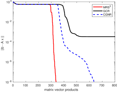
(a) $\alpha=10^{-6}$, $\gamma=1$, $\kappa=4\cdot 10^{7}$

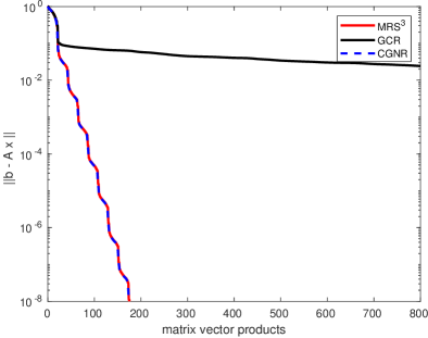
(b) $\alpha=10^{-5}$, $\gamma=100$, $\kappa=15$

Figure 1: Convergence of MRS³, GCR and CGNR

5.2 Numerical comparison of MRS³, GMRES(3) and Bi-CGSTAB

We compare MRS³ with the general Krylov methods GMRES and Bi-CGSTAB. In order to make the memory and work requirements comparable we use GMRES(3), which means that GMRES is restarted every 3 iterations. In our experiments we have also checked that full GMRES indeed leads to the same numerical results as MRS³.

As expected, our experiments show that GMRES(3) and Bi-CGSTAB do not perform very well for SSS systems compared to MRS³, see Figures 2(a) and 2(b). With respect to Bi-CGSTAB, we should note that for these problems BiCGStab2 [13] and Bi-CGSTAB($\ell$) [27] may be better alternatives.

(a) $\alpha=10$, $\gamma=1$, $\kappa=4$

(b) $\alpha=10^{-3}$, $\gamma=1$, $\kappa=4\cdot 10^{4}$

Figure 2: Convergence of MRS³, GMRES(3) and Bi-CGSTAB

5.3 Numerical comparison of MRS³ and CGW

For well-conditioned systems, numerical experiments confirm the theoretical prediction (30) of the CGW residual norm. For such systems CGW performs very well, even though if $\alpha$ is small the peaks in the CGW residual norm history become very large, as demonstrated in Figure 3(a). This is because for small $\alpha$, every other iteration minimal residual methods nearly stagnate, leading to a peak in the CGW residual norm in concurrence with the peak-plateau connection described in Section 4.

For less well-conditioned systems, in practice, CGW can no longer keep up with the theoretical residual norm. This leads to slower convergence, as shown in Figure 3(b), and eventually divergence, where MRS³ still performs well.

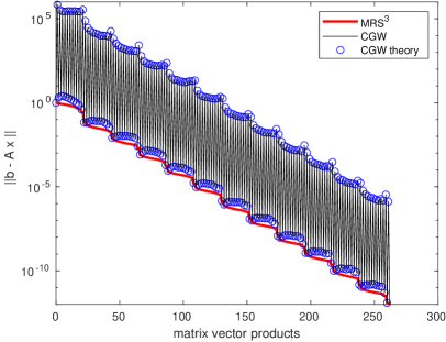
(a) $\alpha=10^{-3}$, $\gamma=100$, $\kappa=15$

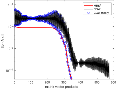
(b) $\alpha=10^{-3}$, $\gamma=1$, $\kappa=4\cdot 10^{3}$

Figure 3: Convergence of MRS³, and CGW

6 Conclusions

We started this paper by showing the importance of a fast solver for shifted skew-symmetric matrix systems (1), (2). Theory by Voevodin [32] and Faber and Manteuffel [8], [9] demonstrates that an algorithm that is optimal and uses short recurrences should exist, however there was no such algorithm available yet, that works for all values of $\alpha$. We have presented such an algorithm, the MRS³ solver.

By theory and numerical experiments, we have shown that the MRS³ method generally outperforms its alternatives. As a minimal residual method it converges faster and is more robust than Galerkin methods, like the CGW algorithm, that do not satisfy the optimality property. At the same time MRS³ also allows $\alpha=0$, where CGW does not.

Full GMRES converges as fast as MRS³ but is not a valid option due to its complexity, whereas restarted GMRES variants have good complexity but cannot maintain the fast convergence. For the specific problem of SSS systems Bi-CGSTAB seems to converge slowly, especially if the system is ill-conditioned, while the complexity is worse than that of MRS³ too.

Truncated GCR performs really well for large $\alpha$, and rivals the complexity of MRS³. However for small $\alpha$ and $\alpha=0$, the GCR algorithm breaks down. The performance of the CGNR method is comparable to that of MRS³ for many problems, but it breaks down for ill-conditioned system that MRS³ can still handle.

We conclude that the proposed MRS³ solver performs very well for the important class of shifted skew-symmetric matrix systems. The complexity of the algorithm is very good, it converges very fast, and it can be used for all values of $\alpha$. Especially for small $\alpha$, or $\alpha=0$, and for ill-conditioned systems, MRS³ performs a lot better than the existing alternatives.

References

• [1] W.E. Arnoldi. The principle of minimized iteration in the solution of the matrix eigenvalue problem. Quart. Appl. Math., 9:17–29, 1951.
• [2] Z. Bai, G.H. Golub, and M.K. Ng. Hermitian and skew-Hermitian splitting methods for non-Hermitian positive definite linear systems. SIAM J. Matrix Anal. Appl., 24:603–626, 2003.
• [3] J. Chen and Z. Shen. Regularized conjugate gradient method for skew-symmetric indefinite systems of linear equations and applications. Applied Mathematics and Computation, 187:1484–1494, 2007.
• [4] P. Concus and G.H. Golub. A generalized conjugate gradient method for nonsymmetric systems of linear equations. In R. Glowinski and J.L. Lions, editors, Lecture Notes in Economics and Mathematical Systems, volume 134, pages 50–56. Springer-Verlag, Berlin, 1976.
• [5] J.K. Cullum. Peaks, plateaus, numerical instabilities in a Galerkin minimal residual pair of methods for solving $Ax=b$. Appl. Numer. Math., 19:255–278, 1995.
• [6] S.C. Eisenstat. A note on the generalized conjugate gradient method. SIAM J. Numer. Anal., 20:358–361, 1983.
• [7] S.C. Eisenstat, H.C. Elman, and M.H. Schultz. Variational iterative methods for nonsymmetric systems of linear equations. SIAM J. Numer. Anal., 20(2):345–357, 1983.
• [8] V. Faber and T. Manteuffel. Necessary and sufficient conditions for the existence of a conjugate gradient method. SIAM J. Numer. Anal., 21:352–362, 1984.
• [9] V. Faber and T. Manteuffel. Orthogonal error methods. SIAM J. Numer. Anal., 24:170–187, 1987.
• [10] G.H. Golub and D. Vanderstraeten. On the preconditioning of matrices with skew-symmetric splittings. Numerical Algorithms, 25:223–239, 2000.
• [11] G.H. Golub and A.W. Wathen. An iteration for indefinite systems and its application to the Navier-Stokes equations. SIAM J. Sci. Comput., 19:530–539, 1998.
• [12] C. Greif and J.M. Varah. Iterative solution of skew-symmetric linear systems. SIAM J. Matrix Anal. Appl., 31(2):584–601, 2009.
• [13] M.H. Gutknecht. Variants of BICGSTAB for matrices with complex spectrum. SIAM J. Sci. Comput., 14(5):1020–1033, 1993.
• [14] M.H. Gutknecht and M. Rozložník. By how much can residual minimization accelerate the convergence of orthogonal residual methods? Numer. Algorithms, 27:189–213, 2001.
• [15] M.H. Gutknecht and M. Rozložník. A framework for generalized conjugate gradient methods—with special emphasis on contributions by Rüdiger Weiss. Appl. Numer. Math., 41:7–22, 2002.
• [16] Y. Huang, A.J. Wathen, and L. Li. An iterative method for skew-symmetric systems. Information, 2:147–153, 1999.
• [17] T. Huckle. The Arnoldi method for normal matrices. SIAM J. Matrix Anal. Appl., 15(2):479–489, 1994.
• [18] R. Idema and C. Vuik. A minimal residual method for shifted skew-symmetric systems. Report 07-09, Delft University of Technology, Delft Institute of Applied Mathematics, 2007.
• [19] E. Jiang. Algorithm for solving shifted skew-symmetric linear system. Front. Math. China, 2:227–242, 2007.
• [20] E. Jiang. Linear port-Hamiltonian descriptor systems. Mathematics of Control, Signals, and Systems, 30, 2018.
• [21] C. Lanczos. An iteration method for the solution of the eigenvalue problem of linear differential and integral operators. J. Res. Natl. Bur. Stand., 45:255–282, 1950.
• [22] C.C. Paige and M.A. Saunders. Solution of sparse indefinite systems of linear equations. SIAM J. Numer. Anal., 12:617–629, 1975.
• [23] C.C. Paige and M.A. Saunders. LSQR: An algorithm for sparse linear equations and sparse least squares. A.C.M. Trans. Math. Softw., 8:43–71, 1982.
• [24] C. Roos, T. Terlaky, and J.-Ph. Vial. Theory and Algorithms for Linear Optimization: An Interior Point Approach. John Wiley & Sons, New York, 1997.
• [25] Y. Saad. Iterative Methods for Sparse Linear Systems. SIAM, second edition, 2003.
• [26] Y. Saad and M.H. Schultz. GMRES: A generalized minimal residual algorithm for solving nonsymmetric linear systems. SIAM J. Sci. Stat. Comput., 7:856–869, 1986.
• [27] G.L.G. Sleijpen, H.A. van der Vorst, and D.R. Fokkema. ${\rm BiCGstab}(l)$ and other hybrid Bi-CG methods. Numer. Algorithms, 7:75–109, 1994.
• [28] H.A. van der Vorst. Bi-CGSTAB: a fast and smoothly converging variant of Bi-CG for solution of non-symmetric linear systems. SIAM J. Sci. Stat. Comput., 13:631–644, 1992.
• [29] H.A. van der Vorst and C. Vuik. The superlinear convergence behaviour of GMRES. J. Comp. Appl. Math., 48:327–341, 1993.
• [30] H.A. van der Vorst and C. Vuik. GMRESR: a family of nested GMRES methods. Num. Lin. Alg. Appl., 1:369–386, 1994.
• [31] P.K.W. Vinsome. Orthomin, an iterative method for solving sparse sets of of simultaneous linear equations. In Proc. Fourth Symposium on Reservoir Simulation, pages 149–159. Society of Petroleum Engineers of AIME, 1976.
• [32] V. V. Voevodin. The problem of non-self-adjoint generalization of the conjugate gradient method is closed. U.S.S.R. Comput. Math. and Math. Phys., 22:143–144, 1983.
• [33] H.F. Walker. Residual smoothing and peak/plateau behavior in Krylov subspace methods. Appl. Numer. Math., 19:279–286, 1995.
• [34] O. Widlund. A Lanczos method for a class of nonsymmetric systems of linear equations. SIAM J. Numer. Anal., 15:801–812, 1978.