Universality of global asymptotics of Jack-deformed random Young diagrams at varying temperatures

Abstract.

This paper establishes universal formulas describing the global asymptotics of two different models of discrete $\beta$-ensembles in high, low and fixed temperature regimes. Our results affirmatively answer a question posed by the second author and Śniady.

We first consider the Jack measures on Young diagrams of arbitrary size, which depend on the inverse temperature parameter $\beta>0$ and specialize to Schur measures when $\beta=2$. We introduce a class of Jack measures of Plancherel-type and prove a law of large numbers and central limit theorem in the aforementioned three regimes. In each regime, we provide explicit formulas for polynomial observables of the limit shape and the Gaussian fluctuations around the limit shape. These formulas have surprising positivity properties and are expressed in terms of weighted lattice paths. We also establish connections between these measures and the work of Kerov–Okounkov–Olshanski on Jack-positive specializations and show that this is a rich class of measures parametrized by the elements in the Thoma cone.

Second, we show that the formulas from limits of Plancherel-type Jack measures are universal: they also describe the limit shape and Gaussian fluctuations for the second model of random Young diagrams of a fixed size defined by Jack characters with the approximate factorization property studied by the second author and Śniady. Finally, we discuss the limit shape in the high/low-temperature regimes and show that, contrary to the continuous case of $\beta$-ensembles, there is a phase transition phenomenon in passing from the fixed temperature regime to the high/low temperature regimes. We note that the relation we find between the two different models of random Young diagrams appears to be new, even in the special case of $\beta=2$ that relates Schur measures to the character measures with the approximate factorization property studied by Biane and Śniady.

1. Introduction and main results

1.1. Jack-deformed random Young diagrams as discrete $\beta$-ensembles

The Gaussian Unitary Ensemble (GUE) is one of the most well-studied models of random matrices. The joint density of eigenvalues $x_{1}>\dots>x_{N}$ of the GUE is given by a formula of the form

$$\frac{1}{Z_{\beta,N,V}}\prod_{1\leq i<j\leq N}|x_{i}-x_{j}|^{\beta}\prod_{i=1}^{N}\exp(-V(x_{i})),$$

where $\beta=2,\,V(x)=\frac{x^{2}}{2}$, and $Z_{\beta,N,V}$ is the normalization constant. When we choose an arbitrary $\beta>0$ and $V(x)=\frac{x^{2}}{2}$, we obtain the joint density of eigenvalues of the model of random matrices known as the Gaussian $\beta$-Ensemble (G$\beta$E). For generic $V(x)$ and arbitrary $\beta>0$, this model is known in probability as a $\beta$-ensemble and in classical statistical mechanics as a one-dimensional log-gas system of $N$ particles in a potential $V$ at inverse temperature $\beta>0$ [For10].

While the asymptotic behavior as $N\to\infty$ of $\beta$-ensembles is well understood for a fixed $\beta>0$ (see for instance [BAG97, Joh98, DE02, VV09, RRV11]), the asymptotic analysis of $\beta$-ensembles in the high-temperature regime in which $N\rightarrow\infty$ and $\beta\rightarrow 0$ simultaneously with $N\beta\sim c$ for some constant $c$ has recently gained a lot of attention in the literature [ABG12, BGP15, DS15, NT18, AB19, Pak20, HL21, For22, BGCG22].

It is well understood by now that the remarkable asymptotic properties of GUE as $N\to\infty$ are reflected in the asymptotics of its discrete counterpart, given by the Plancherel measure on Young diagrams [VK77, LS77, BDJ99, BOO00, Oko00, IO02], see e.g. [BDS16] and references therein. This measure has a natural one-parameter deformation, introduced by Kerov [Ker00], and called the Jack–Plancherel measure. By definition, the Jack–Plancherel measure is the probability measure on the set $\mathbb{Y}_{d}$ of Young diagrams of a fixed size $d\in\mathbb{Z}_{\geq 0}$ that depends on the Jack deformation parameter $\alpha>0$ and is given by the formula

(1) $$\mathbb{P}^{(\alpha)}_{d}(\lambda):=\frac{d!\,\alpha^{d}}{\prod_{(i,j)\in\lambda}\big{(}\alpha(\lambda_{i}-j)+(\lambda_{j}^{\prime}-i)+1\big{)}\big{(}\alpha(\lambda_{i}-j)+(\lambda_{j}^{\prime}-i)+\alpha\big{)}}.$$

It was expected (see e.g. [Oko03]) that the Jack–Plancherel measure would provide a natural discrete analogue of the Gaussian $\beta$-Ensemble, analogous to the discrete counterpart of GUE provided by the Plancherel measure. The parameter $\alpha$ is related to the inverse temperature $\beta>0$ of log-gas systems with potential $V(x)=\frac{x^{2}}{2}$ by the relation $\alpha=2/\beta$. This prediction was confirmed in several ways, for instance, the second author and Féray proved in [DF16] the LLN and CLT for random Jack–Plancherel Young diagrams and conjectured that the edge scaling limit is given by the $\beta$-Tracy–Widom law; this conjecture was later proved by Guionnet and Huang [GH19].

In the last two decades, different models for discrete $\beta$-ensembles which are analogs of the continuous $\beta$-ensembles with a generic potential $V$, and which are far-reaching generalizations of the Jack–Plancherel measure, have been proposed by various authors. It turns out that all these models are significantly different, and the exact and asymptotic methods developed for their analyses are different as well.

The first models are the Jack measures on Young diagrams of arbitrary size; they are defined as the natural $\alpha$-deformations of Okounkov’s Schur measures [Oko01], and as distinguished specializations of the Macdonald measures of Borodin–Corwin [BC14]. The study of Jack measures was first suggested by Borodin and Olshanski in their paper  [BO05] on $1$-parameter deformations of the $z$-measures from the representation theory of the infinite symmetric group [BO17], and were first studied in general by the third author in [Mol23]. Jack measures are probability measures on the infinite set of all Young diagrams $\mathbb{Y}$ defined by two homomorphisms $\rho_{1},\rho_{2}:\operatorname{Sym}\to\mathbb{C}$ from the real algebra of symmetric functions $\operatorname{Sym}$ to the complex numbers. Denote the power-sum symmetric functions by $p_{1},p_{2},\dots$, and the Jack symmetric functions by $J^{{(\alpha)}}_{\lambda}$. Under the normalization and nonnegativity conditions

(2) $$\sum_{k\geq 1}\frac{\rho_{1}(p_{k})\overline{\rho_{2}(p_{k})}}{k}<\infty,\qquad\rho_{1}\left(J_{\lambda}^{(\alpha)}\right)\overline{\rho_{2}\left(J_{\lambda}^{(\alpha)}\right)}\geq 0,\quad\forall\,\lambda\in\mathbb{Y},$$

the Jack measure $M_{\rho_{1},\rho_{2}}^{(\alpha)}$ is defined by the formula

(3) $$M_{\rho_{1},\rho_{2}}^{(\alpha)}(\lambda):=\frac{\rho_{1}\left(J_{\lambda}^{(\alpha)}\right)\overline{\rho_{2}\left(J_{\lambda}^{(\alpha)}\right)}}{j^{(\alpha)}_{\lambda}}\exp\left(-\sum_{k=1}^{\infty}{\frac{\rho_{1}(p_{k})\overline{\rho_{2}(p_{k})}}{k\alpha}}\right),\quad\lambda\in\mathbb{Y}.$$

A second model, introduced by the second author and Śniady [DS19], defines probability measures on the finite set of Young diagrams $\mathbb{Y}_{d}$ of a fixed size $d$. These measures $\mathbb{P}^{(\alpha)}_{\chi_{d}}$ are defined by the decomposition of a general choice of reducible Jack character $\chi_{d}:\mathbb{Y}_{d}\to\mathbb{C}$ into a convex combination of irreducible Jack-characters $\chi^{(\alpha)}_{\lambda}$:

(4) $$\chi_{d}=\sum_{\lambda\in\mathbb{Y}_{d}}\mathbb{P}^{(\alpha)}_{\chi_{d}}(\lambda)\ \chi^{(\alpha)}_{\lambda}.$$

The irreducible Jack characters are defined as the normalized coefficients of the Jack polynomial $J_{\lambda}^{{(\alpha)}}$ expressed in the power-sum basis $p_{\mu}$, and they coincide with the normalized irreducible characters of the symmetric groups in the special case $\alpha=1$ (see Section 2 for more details). In particular, the case $\alpha=1$ recovers measures considered by Biane [Bia01] and Śniady [Śni06], which arise in the context of the asymptotic representation theory of the symmetric group and free probability theory.

The last model we will mention is the one introduced by Borodin, Gorin and Guionnet [BGG17], consist of the discrete $\beta$-ensembles, defined as certain probability measures on the infinite set $\mathbb{Y}^{(N)}$ of Young diagrams with a fixed number $N$ of rows. The key insight in [BGG17] is that one can modify the formula for the joint density of eigenvalues $x_{N}<\dots<x_{1}$ of continuous $\beta$-ensembles to produce a discrete version whose correlation functions satisfy a discrete analog of the loop equations. For $\beta=2$, these 1d models appear as marginals of several models from 2d statistical mechanics such as random tilings, stochastic systems of non–intersecting paths, and last passage percolation.

These discrete variants of $\beta$-ensembles have different origins and observe that they are even supported on slightly different spaces, namely $\mathbb{Y}$, $\mathbb{Y}_{d}$ and $\mathbb{Y}^{(N)}$. Remarkably, the asymptotic behaviors of large Young diagrams sampled from each of them admit clean analyses and descriptions. The third author proved a weak version of LLN and CLT for certain specialization of Jack measures in high, low, and fixed temperature regimes under certain regularity assumptions [Mol23], provided that pairs of specializations which satisfy the nonnegativity assumption in (2) exist. Verifying the latter statement is a priori a difficult problem, except for the special class of Jack measures $M_{\rho,\rho}$ with the same specializations $\rho_{1}=\rho_{2}=:\rho$, for which (2) is trivially satisfied. The third author used this fact to give an analytic description of the limit shape and Gaussian process in this case. Next, in the work of the second author and Śniady [DS19], the authors prove a LLN and CLT for large random Young diagrams sampled by the measures $\mathbb{P}^{(\alpha)}_{\chi_{d}}$, when $(\chi_{d})_{d\geq 1}$ is a sequence of Jack characters satisfying the approximate factorization property (see Section 2 for precise definitions). In the special case $\alpha=1$, it corresponds to the LLN for random representations of large symmetric groups studied by Biane [Bia01] and the CLT for those representations proved by Śniady [Śni06]. Finally, for the discrete $\beta$-ensembles of Borodin–Gorin–Guionnet [BGG17], the authors prove a LLN and CLT in the fixed temperature regime under certain regularity conditions on the potential $V$ via certain discrete loop equations.

Our understanding of the relations between all these models was limited to the simple fact that their intersection includes (not directly, though) the Jack–Plancherel measure in (1). The problem of finding an intrinsic relation between these models and their methods of analysis has been suggested to us on several occasions by experts in the field, and the second author proposed it already in his joint work with Śniady [DS19, Section 1.3]. In this paper, we take a step forward in this direction, by establishing a deep connection between the first two models mentioned previously (Jack measures and Jack character measures with the asymptotic factorization property). Specifically, we find a very large infinite-parameter family of measures, called the Plancherel-type Jack measures, and their depoissonized versions which fit into both settings. We prove that the global asymptotic behavior of these measures is governed by explicit formulas expressed in terms of simple and elegant combinatorial objects known as lattice paths. Furthermore, we show that this special family of measures is dense enough so that actually all Jack character measures with the AFP display the same universal global-scale behavior. The path to this surprising discovery was intricate, and we describe each step of our journey in detail, presenting a series of novel results along the way.

1.2. Main result for Jack measures

Our first main results describe the asymptotic behavior of certain Jack measures via explicit combinatorial formulas. Let $\alpha>0$, $\mathbf{v}=(v_{1},v_{2},\cdots)\in\mathbb{R}^{\infty}$, and $u>0$. We say that the Jack measure

(5) $$M^{(\alpha)}_{u;\mathbf{v}}(\lambda):=\exp\left(-\frac{u^{2}\cdot v_{1}}{\alpha}\right)\frac{J_{\lambda}^{(\alpha)}(u\cdot\mathbf{v})\cdot u^{|\lambda|}}{j^{(\alpha)}_{\lambda}},\quad\forall\,\lambda\in\mathbb{Y},$$

is of Plancherel-type and corresponds to the Jack measure $M_{\rho_{1},\rho_{2}}$ in (3) with the following choice of specializations: $\rho_{1}(p_{k})=u\cdot v_{k}$ and $\rho_{2}(p_{k})=u\cdot\delta_{1,{k}}$, for all ${k}\geq 1$. The nonnegativity assumption in (2) is no longer automatically satisfied, as it was for the special case of $M_{\rho,\rho}$ studied in [Mol23]. For our Plancherel-type Jack measures, and for a fixed $\alpha>0$, the nonnegativity assumption reduces to the classification of $\alpha$-Jack-positive specializations of $\operatorname{Sym}$. Such a classification was completed by Kerov, Okounkov and Olshanski in [KOO98], where they extended the celebrated Thoma’s classification of extremal characters of the infinite symmetric group (see [Tho64, KOO98, Mat19]). Based on their result, $M^{(\alpha)}_{u;\mathbf{v}}$ defines a probability measure on the set $\mathbb{Y}$ of partitions of arbitrary size whenever $u,\mathbf{v}$ are points parametrized by the points from the Thoma cone

$$\Omega=\{(a,b,c)\in\mathbb{R}^{\infty}\times\mathbb{R}^{\infty}\times\mathbb{R}\mid a=(a_{1},a_{2},\cdots),\quad b=(b_{1},b_{2},\cdots),\\ a_{1}\geq a_{2}\geq\cdots\geq 0,\quad b_{1}\geq b_{2}\geq\cdots\geq 0,\quad\sum_{i=1}^{\infty}{(a_{i}+b_{i})}\leq c\}$$

by setting $v_{1}=u^{-1}\cdot c$ and $v_{k}=u^{-1}\sum_{i=1}^{\infty}a_{i}^{k}+u^{-1}(-\alpha)^{1-k}\sum_{i=1}^{\infty}b_{i}^{k}$, for $k\geq 2$, and $u>0$ is arbitrary. This shows that the class of Plancherel-type Jack measures is a rich infinite-parameter family. Moreover, except for the Jack–Plancherel measure that belongs to both classes $M_{\rho,\rho}$ and $M^{(\alpha)}_{u;\mathbf{v}}$, these two classes are disjoint. Hence, next to the previously studied $M_{\rho,\rho}$, the Jack measures of Plancherel-type form the most natural class of Jack measures that can be studied.

We are interested in the behavior of $M^{(\alpha)}_{u;\mathbf{v}}$-distributed Young diagrams for a generic choice of the infinite family of parameters $\mathbf{v}=(v_{1},v_{2},\cdots)\in\mathbb{R}^{\infty}$ as the ratio $\frac{\alpha}{u^{2}}$ tends to zero. This asymptotic regime describes the typical behavior of a large $M^{(\alpha)}_{u;\mathbf{v}}$-distributed random Young diagram. We study the asymptotic behavior of $M^{(\alpha)}_{u;\mathbf{v}}$ in three different regimes: the fixed temperature regime when $\frac{\alpha-1}{u}\to 0$ (for instance when $\alpha>0$ is fixed and $u\to\infty$), the high temperature regime when $\frac{\alpha-1}{u}\to g>0$, and the low temperature regime when $\frac{\alpha-1}{u}\to g<0$. Therefore, in this subsection assume that $\alpha=\alpha(d)$, $u=u(d)$ are sequences of positive real numbers such that

(6) $$\lim_{d\to\infty}\frac{\alpha}{u^{2}}=0,\qquad\lim_{d\to\infty}\frac{\alpha-1}{u}=g\in\mathbb{R},\qquad M^{(\alpha)}_{u;\mathbf{v}}(\lambda)\geq 0,\quad\forall\,\lambda\in\mathbb{Y},\ \forall\,d\in\mathbb{Z}_{\geq 0}.$$

Note that in the case when $g\neq 0$ (the high and low temperature regimes), it is quite nontrivial to find sequences $\alpha,u$ that satisfy the conditions (6), with the nonnegativity of $M^{(\alpha)}_{u;\mathbf{v}}$ being especially troublesome. When $g=0$ and $\alpha>0$ is fixed, we noted that [KOO98] furnishes examples where $v_{k}$ depends on $\alpha$; however, this becomes an issue if $\alpha$ varies, because the parameters $v_{k}$ must remain constant. Nevertheless, we manage to find a large family of pairs $(g,\mathbf{v})\in(\mathbb{R}\setminus\{0\})\times\mathbb{R}^{\infty}$ for which these conditions are satisfied, see Definition 4.5 and Proposition 4.6. Our construction is based on a new classification theorem for totally Jack-positive specializations, see Theorem 4.4, i.e. specializations which take nonnegative values on all Jack symmetric functions $J^{(\alpha)}_{\lambda}$, for all $\alpha>0$.

In our first main limit theorem, we prove that the profile $\omega_{\Lambda_{(\alpha;u\cdot\sqrt{v_{1}})}}$ of a properly rescaled random Young diagram $\Lambda_{(\alpha;u)}$, obtained from a Young diagram $\lambda$ by replacing each box of size $1\times 1$ by a box of size $\frac{\alpha}{u\cdot\sqrt{v_{1}}}\times\frac{1}{u\cdot\sqrt{v_{1}}}$, concentrates around a deterministic shape, and this holds true in all three limit regimes. As a side comment we mention that we deduce this result from a general statement about the convergence of random functions (see Theorem 3.15) that might be helpful in a wide variety of similar contexts, and is of independent interest. Here is the abbreviated version of our first main result (see Theorem 3.7 for the detailed version).

Theorem 1.1.

Fix $g\in\mathbb{R}$ and $\mathbf{v}=(v_{1},v_{2},\cdots)\in\mathbb{R}^{\infty}$. Suppose that $\alpha,u\in\mathbb{R}_{>0}$ satisfy (6). Then there exists some deterministic function $\omega_{\Lambda_{g;\mathbf{v}}}\colon\mathbb{R}\to\mathbb{R}$ with the property that

(7) $$\lim_{d\rightarrow\infty}\omega_{\Lambda_{(\alpha;u\cdot\sqrt{v_{1}})}}=\omega_{\Lambda_{g;\mathbf{v}}}.$$

The limit in (7) means convergence with respect to the supremum norm in probability. Moreover, the limit shape $\omega_{\Lambda_{g;\mathbf{v}}}$ is described by explicit formulas for various observables that uniquely determine it (see (8) below for the moments of the associated transition measure, and (73) for the moments of the measure with the density $\frac{\omega_{\Lambda_{g;\mathbf{v}}}(x)-|x|}{2}$). These formulas are expressed in terms of a weighted enumeration of Łukasiewicz paths.

Informally, a Łukasiewicz path is a directed lattice path with steps $(1,k),\,k\in\mathbb{Z}_{\geq-1}$, starting at $(0,0)$ and finishing at $(\ell,0)$ that stays in the first quadrant. These objects are in bijection with non-crossing set partitions, a combinatorial model intrinsically related to free probability (see Remark 9 and the discussion in Section 1.3). Consider the following weighted generating series for the set $\mathbf{L}_{0}(\ell)$ of Łukasiewicz paths of length $\ell$:

(8) $$M_{\ell}:=v_{1}^{-\ell/2}\cdot\sum_{\Gamma\in\mathbf{L}_{0}(\ell)}{\prod_{i\geq 0}(ig)^{\text{number of horizontal steps at height $i$}}\cdot\prod_{j\geq 1}v_{j}^{\text{number of steps $(1,j)$}}}.$$

We prove that the $\ell$-th moment of the transition measure $\mu_{\Lambda_{g;\mathbf{v}}}$ associated with the limit shape $\omega_{\Lambda_{g;\mathbf{v}}}$ via the Markov–Krein correspondence is given by this series:

$$\int_{\mathbb{R}}{x^{\ell}\mu_{g;\mathbf{v}}(dx)}=M_{\ell},\quad\text{for all $\ell\geq 1$}.$$

Note that in the special case when $g=0$ (e.g. when $\alpha>0$ is fixed), $\mathbf{v}=(1,0,0\dots)$ and $\mathbf{v}=(1,c,c^{2},\dots)$, our formula (8) recovers the combinatorial formula for the moments of the semicircle distribution and the free Poisson distribution, respectively. These two special cases correspond to the LLN for the Jack–Plancherel measure ([LS77, VK77] for $\alpha=1$, [DF16] for general $\alpha>0$) and for the Schur-Weyl measure ([Bia01] for $\alpha=1$); the high and low temperature regimes give one-parameter deformations of these laws. In particular, note that when specialized to $\alpha=1,\,g=0$, we provide a new proof of Biane’s result, see Remark 9. Moreover, Plancherel-type Jack measures are distinguished mixtures of the measures on partitions of a fixed size already studied by Kerov, Okounkov and Olshanski [KOO98] in the context of harmonic functions on the Young graph with Jack multiplicities and a fixed $\alpha$. In light of our depoissonization analysis (see Section 1.3), our Theorem 1.1 describes the limit shape for all these measures. We want to point out here that this limit shape is described not only for an arbitrary, but fixed parameter $\alpha$ (which turns out to be the same as in the $\alpha=1$ case studied by Okounkov in [Oko00]), but it also covers the high and low temperature limits of the Kerov–Okounkov–Olshanski measures.

We conclude our analysis of Jack measures of Plancherel-type by proving the central limit theorem. We determine the (non-centered) Gaussian process describing fluctuations around the limit shape by giving explicit formulas for its mean shift and covariance matrix. For technical reasons, we require that the assumptions on the growth of $\alpha$ and $u$ in (6) are slightly enhanced and replaced by $\frac{\alpha}{u^{2}}=\frac{1}{d}+o\left(\frac{1}{d}\right),\frac{\alpha-1}{u}=g+\frac{g^{\prime}}{\sqrt{d}}+o\left(\frac{1}{\sqrt{d}}\right)$, as $d\to\infty$; see Remark 6. This is the abbreviated version (see Theorem 3.8 for the precise statement):

Theorem 1.2.

Fix $g,g^{\prime}\in\mathbb{R}$ and $\mathbf{v}=(v_{1},v_{2},\cdots)\in\mathbb{R}^{\infty}$. Suppose that the sequences of positive reals $\alpha,u$ satisfy the aforementioned enhanced version of (6). Then there exists a Gaussian process $\Delta_{g,g^{\prime};\mathbf{v}}$ such that the random functions $\Delta^{(\alpha)}_{u;\mathbf{v}}:=\frac{u}{\sqrt{\alpha}}\bigg{(}\frac{\omega_{\Lambda_{(\alpha;u\cdot\sqrt{v_{1}})}}-\omega_{\Lambda_{g;\mathbf{v}}}}{2}\bigg{)}$ converge to $\Delta_{g,g^{\prime};\mathbf{v}}$ in distribution for multidimensional polynomial test functions. This process is uniquely determined by (55) that describes its mean vector, and (56) that describes its covariance matrix.

To prove these results, we develop a combinatorial approach to Nazarov–Sklyanin operators, building on the work initiated in [Mol23]. For random partitions distributed according to the Plancherel-type Jack measures, and their transition measures, we can describe various important observables by elegant combinatorial models of Łukasiewicz ribbon paths that we introduce here (e.g. see Theorem 3.10). These combinatorial formulas allowed us to take limits in our regimes of interest and were the basis of our LLN and CLT. Finally, let us reiterate that we are able to construct, in Section 4, a very rich family of specializations with certain positivity properties that lead to valid sequences of measures for which Theorem 1.1 and Theorem 1.2 are applicable in the high and low temperature regimes. These sequences are parametrized by $g\in\mathbb{R}\setminus\{0\}$ and $c\geq a_{1}\geq a_{2}\geq\cdots\geq 0$ with $\sum_{i=1}^{\infty}{a_{i}}\leq c$ (see Theorem 4.4 and Proposition 4.6). These ideas turn out to be a key link between Plancherel-type Jack measures and Jack character measures with the AFP, thus allowing us to establish that the asymptotic behavior of both models is governed by universal formulas expressed in terms of Łukasiewicz ribbon paths.

1.3. Main result for measures with the approximate factorization property.

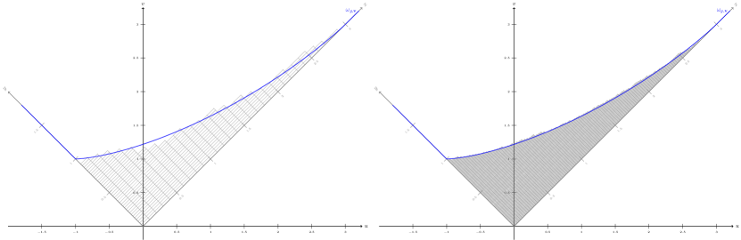
Figure 1. The profile $\omega_{\Lambda^{(\alpha)}_{d}}$ of the anisotropically-scaled Young diagrams of size $d=400$ and $d=6400$ sampled by the Jack–Schur–Weyl measure from Section 2.6.2 with parameters $\alpha=4,\,N=\sqrt{\alpha\cdot d}$, where each box is not of size $1\times 1$, but of size $\frac{2}{\sqrt{d}}\times\frac{1}{2\cdot\sqrt{d}}$. The blue curve is the limit shape $\omega_{\Lambda_{\infty}}$ in the fixed temperature regime (fixed $\alpha>0$), first discovered by Biane [Bia01].

Our second main result relates the previously studied Jack measures with the model introduced by the second author and Śniady in [DS19]. We recall that given a general reducible Jack character $\chi_{d}\colon\mathbb{Y}_{d}\to\mathbb{R}$, we can associate a probability measure on the set of Young diagrams $\mathbb{Y}_{d}$ of size $d$ by the formula (4). The Jack characters $\chi_{d}$ which are interesting from the probabilistic point of view are those which have the approximate factorization property (AFP). Roughly speaking, in the simplest case this property says that the character $\chi_{d}(\pi_{1}\cdot\pi_{2})$, evaluated on the disjoint product of partitions $\pi_{1},\pi_{2}$, behaves asymptotically the same as the product of characters $\chi_{d}(\pi_{1})\cdot\chi_{d}(\pi_{2})$, and similar formulas hold asymptotically for all higher order cumulants; see Section 2 for the precise definitions. The second author and Śniady proved in [DS19] the LLN and CLT for the Jack character measures with the AFP in all three previously discussed regimes (see Theorem 2.3 and Theorem 2.4).

The primary tool used in [DS19] is the rich algebraic structure of Jack characters. This approach, also known as the dual approach, stems from the successful viewpoint of Kerov and Olshanski [KO94], who observed that the set of characters of the symmetric groups, treated as functions on the set of Young diagrams representing the associated irreducible representation, is strictly related to the algebra of shifted symmetric functions. The generalization of this approach to the setting of Jack characters was proposed by Lassalle in [Las08, Las09], who formulated challenging conjectures on various positivity phenomena of Jack characters. Despite significant efforts [DFS14, DF16, Ś19, BD22b], these conjectures remain wide open prior to our work. Consequently, finding formulas for the moments of the limiting transition measure $\mu_{\Lambda_{\infty}}$ from Theorem 2.3 and for the covariance of the Gaussian process $\Delta_{\infty}$ from Theorem 2.4 turned out to be far beyond our reach. Our second main result solves this problem and we show that that the formulas for the moments and for the covariance described in the previous section are in fact universal for both models.

Theorem 1.3 (Abbreviated version of Theorems 5.1 and 5.2).

Assume that $\chi_{d}\colon\mathbb{Y}_{d}\to\mathbb{R}$ are reducible Jack characters such that the sequence $(\chi_{d})_{d\geq 1}$ fulfills the AFP (enhanced AFP, respectively) given by Definition 2.2. Let $\mu_{\Lambda_{\infty}}$ and $\Delta_{\infty}$ be the limiting transition measure and the limiting Gaussian process described by Theorem 2.3 and Theorem 2.4, respectively. Then the moments $M_{\ell}:=\int_{\mathbb{R}}{x^{\ell}\mu_{\Lambda_{\infty}}(dx)}$ are given by the polynomial formula (8), and the mean shift $\mathbb{E}[\langle\Delta_{\infty},\,x^{\ell-2}\rangle]$ and the covariance $\operatorname{Cov}\left(\langle\Delta_{\infty},x^{k-2}\rangle,\langle\Delta_{\infty},x^{l-2}\rangle\right)$ are given by the explicit polynomial formulas (90) and (91), respectively, that are obtained from the universal formulas (55) and (56) by incorporating the terms $v_{k}^{\prime},v_{(k|l)}\,$ from the second order asymptotics of the character $\chi_{d}$ (given by (19)).

Our method for proving Theorem 1.3 synthesizes tools described in the previous section with algebraic tools developed in [DF16, DS19]. We show that the Plancherel-type Jack measures described earlier are, in fact, a Poissonized version of a specific class of examples of measures with the AFP (see Section 2.6.3). This allows us to deduce Theorem 1.3 for this specific class. However, to understand the asymptotic behavior of arbitrary measures with the AFP, we need new ideas. We use the theory developed in [DF16, DS19] to prove that the class of examples from Section 2.6.3 is large enough to ensure that the polynomial formulas described in Theorem 1.3 are universal for the entire class of measures with the AFP.

1.4. Connections to Free Probability Theory and Algebraic Combinatorics

Before delving into direct applications of our formulas, it is worth mentioning some interesting ramifications of our work in related subjects.

Biane’s fundamental work [Bia98] established a connection between asymptotic representation theory of symmetric groups and free probability; we recover this fact because (8) implies that the $v_{k}$’s are the free cumulants of the limiting transition measure $\mu_{\Lambda_{g;\mathbf{v}}}$ when $g=0$, see Remark 9. For a general $g$, the formula (8) defines a novel notion of $g$-deformed free cumulants that we hope to investigate in future works. Other such deformations have appeared previously in the literature, e.g. see [BGCG22, MP22, Nic95]. Ours is more similar to the one in [BGCG22, MP22] because both have, conjecturally, the property that the natural notion of $g$-deformed free convolution is positivity preserving: if $\mu,\nu$ are probability measures, it is conjectured that there exists a probability measure $\mu\boxplus_{g}\nu$ whose $g$-cumulants are the sums of the $g$-cumulants of $\mu$ and $\nu$. This is related to the conjecture of Stanley [Sta89] on the positivity of the structure constants for Jack polynomials. Furthermore, a different positivity of the $g$-deformed free cumulant $v_{k}$ was proved by Śniady [Ś19]: there exists a polynomial $K_{k}(-g,R_{2},R_{3},\dots)$ in $g$ and the free cumulants $R_{2},R_{3},\dots$ with positive integer coefficients, such that $v_{k}=K_{k}(-g,R_{2},R_{3},\dots)$. This polynomial is the top-degree part of the so-called Kerov polynomials, whose positivity was conjectured by Lassalle [Las09] and is still wide open (see also [Fér09, DFŚ10, DF16]). Śniady found a combinatorial interpretation of polynomials $K_{k}$ in terms of graphs embedded into non-oriented surfaces such that the exponent of $g$ is computed by a recursive decomposition of these graphs. In practice, controlling this exponent is almost impossible, except for some special cases, see [DFS14, Doł17, CD22, BD22a]. Comparing to Śniady’s formula, our combinatorial interpretation involves drastically simpler combinatorial objects and, most importantly, the exponent of $g$ is an explicit statistic of the underlying path. Therefore we provide new combinatorial tools to attack Lassalle’s positivity conjectures [Las08, Las09] and they already turned out to be very successful — the second author in a joint work with Ben Dali [BDD23] used the results presented here to prove integrality of the coefficients in Kerov’s polynomials and to fully prove Lassalle’s conjecture from [Las08]. We believe that the tools developed in this paper will lead to ultimate understanding of the Kerov’s polynomials.

1.5. Further applications

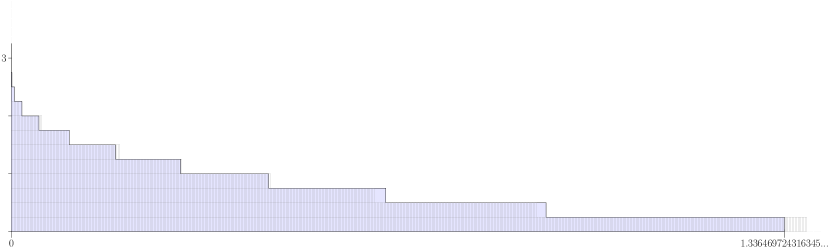
Figure 2. The limit shape $\Lambda_{g;(1,0,0,\cdots)}$ with $g\!=\!-\frac{1}{4}$ (low temperature regime), $\mathbf{v}\!=\!(1,0,0,\cdots)$ is shaded in light blue. Juxtaposed is the anisotropically scaled Young diagram of size $d=1600$ sampled by the Jack–Plancherel measure $\mathbb{P}^{(\alpha)}_{d}$ with $\alpha=\frac{4^{2}}{d}$, where each box (with gray-colored sides) is not of size $1\!\times\!1$, but of size $\frac{4}{d}\!\times\!\frac{1}{4}$. In this concrete example, computer calculations helped us determine that $\lim_{d\to\infty}\frac{\lambda_{1}}{-g\cdot d}=1.33646...$ in probability.

Theorem 1.1 implies that the limit shape $\omega_{\Lambda_{g;\mathbf{v}}}$ in the fixed temperature regime (i.e., when $g=0$) does not depend on the choice of $\alpha>0$, as long as it is fixed, and is the same as in the classical setting when $\alpha=1$. In this case, the limit shape is balanced, meaning that $\omega_{\Lambda_{g;\mathbf{v}}}(x)=|x|$ for $x$ large enough. However, in the high and low temperature regimes, i.e., when $g>0$ and $g<0$, respectively, the situation is different.

Drawing an analogy with recent studies on the high and low temperature regimes of log-gases (see Section 1.1), we apply our combinatorial formulas to study the limit shape $\omega_{\Lambda_{g;\mathbf{v}}}$ (or equivalently, the associated transition measure $\mu_{g;\mathbf{v}}$) in the high and low temperature regimes. We show that, unlike in the continuous counterpart of log-gases, there is a phase transition in our models when transitioning from the fixed temperature regime to the high and low temperature regimes. Specifically, we prove that for $g\neq 0$, the measure $\mu_{g;\mathbf{v}}$ is discrete on $\mathbb{R}$ with an infinite support bounded only on one side and with a unique accumulation point at $+\infty$ or $-\infty$, depending on the sign of $g$ (see Propositions 6.5 and 6.6, and compare Fig. 2 to Fig. 1).

Finally, we relate $\mu_{g;\mathbf{v}}$ to a specific unbounded Toeplitz-like matrix, and we use it to describe the edge asymptotics of the random partitions. By analogy with the celebrated works of Baik, Borodin, Deift, Johanson, Okounkov, Olshanski [BDJ99, BOO00, Oko00] on the relation between the asymptotics of the largest rows of Plancherel-sampled Young diagrams and the asymptotics of the largest eigenvalues of GUE, we study the special case when $\mathbf{v}=(1,0,0,\cdots)$, and prove the following theorem, which relates the asymptotics of the largest rows of Jack–Plancherel-sampled Young diagrams with the asymptotics of the largest eigenvalues of finite deterministic Jacobi matrices (here we only state the abbreviated version for low temperature, i.e. for $g<0$; see Theorem 6.12 for the more general statement and Fig. 2 to see the limit shape drawn with the help of this theorem).

Theorem 1.4.

Let $(\lambda^{(d)}\in\mathbb{Y}_{d})_{d\geq 1}$ be a sequence of random Young diagrams distributed by the Jack–Plancherel measures. In the regime $d,\alpha^{-1}\to\infty,\,\sqrt{\alpha d}\to-g^{-1}>0$, for any $i=1,2,\cdots$, we have

$$\frac{\lambda^{(d)}_{i}}{-g\cdot d}\longrightarrow\lim_{N\to\infty}l_{i}^{(g,N)}-(i-1)g\quad\text{in probability,}$$

where $l_{1}^{(g,N)}>\dots>l_{N}^{(g,N)}$ are the eigenvalues of the $N\times N$ Jacobi matrix $J^{N}_{g;\mathbf{v}}=[(J^{N}_{g;\mathbf{v}})_{i,j}]_{\,i,j=0}^{N-1}\,$ defined by $(J^{N}_{g;\mathbf{v}})_{i,j}:=ig\cdot\delta_{i,j}+\delta_{1,|j-i|}$.

1.6. Organization of the paper

In Section 2, we review the definition of Jack characters with the AFP, their associated probability measures, and we restate the LLN and CLT obtained in [DS19]. We also give a large family of examples relating this model to the Plancherel-type Jack measures. The latter model is introduced in Section 3, where we also prove our first main theorems: the LLN and CLT for the Plancherel-type Jack measures. Section 4 is devoted to study Jack-positive specializations in different regimes and relating our new family of measures with the Thoma cone. In Section 5, we prove our second main theorem: first we show that the conditional Plancherel-type Jack measure fits into the model of Jack-characters with the AFP, and second we study the algebraic structure of Jack characters in order to deduce formulas for the moments of the limiting measure and for the mean shift and covariance of the limiting Gaussian process. The last Section 6 is devoted to the study of the limit shape, as well as its transition measure, arising from the high and low temperature limits of random partitions.

2. First model of random Young diagrams: Jack characters and the asymptotic factorization property

In this section and the next, we review two different constructions of probability measures on the set of Young diagrams that depend on the Jack parameter, and that were introduced in [DS19, Mol23]. It turns out that these two a priori different models are intimately related (see e.g. Proposition 5.3), and this relation will be exploited later in Section 5. In this section, we review the construction from [DS19] that yields probability measures on the finite set $\mathbb{Y}_{d}$ of Young diagrams of a fixed size $d$, and is inspired by the relation between symmetric functions and the representation theory of symmetric groups; see [Bia01, Śni06]. We also review the LLN and CLT as the size $d$ of the partitions tends to infinity.

2.1. Asymptotics of the Jack parameter

In this paper, we employ the Jack parameter, classically denoted by $\alpha>0$. Later in this section, when we state our limit theorems, we will have instead a sequence $(\alpha(d))_{d\geq 1}$ of Jack parameters, i.e. of positive real numbers. To simplify our notation, a general term of this sequence will be denoted by $\alpha=\alpha(d)$. We will assume that

(9) $$\frac{\sqrt{\alpha}-\frac{1}{\sqrt{\alpha}}}{\sqrt{d}}=g+\frac{g^{\prime}}{\sqrt{d}}+o\left(d^{-\frac{1}{2}}\right),\ \text{ as }d\to\infty,$$

for some constants $g,g^{\prime}\in\mathbb{R}$.

The regime when $g>0$ and $\alpha,\,d$ are of the same order, i.e. $\alpha=\Theta(d)$ (resp. $g<0$ and $\alpha=\Theta(d^{-1})$) is called the high temperature regime (resp. low temperature regime). Likewise, the regime when $g=0$, $\,\alpha=\Theta(1)$ and $g^{\prime}=\sqrt{\alpha}-\frac{1}{\sqrt{\alpha}}$ is called the fixed temperature regime.

2.2. Conditional cumulants

Let $\mathbb{Y}_{d}$ denote the set of partitions (equivalently, Young diagrams) of $d\in\mathbb{Z}_{\geq 0}$, and let $\mathbb{Y}:=\bigsqcup_{d\geq 0}{\mathbb{Y}_{d}}$ be the set of all partitions. For any $\mu,\mu^{\prime}\in\mathbb{Y}$, we define their product $\mu\cdot\mu^{\prime}$ as their union, for example $(4,2,1)\cdot(5,3,1)=(5,4,3,2,1,1)$. In this way, the set of all partitions $\mathbb{Y}$ becomes a unital semigroup with the unit being the empty partition $\emptyset$. The corresponding semigroup algebra of formal linear combinations of partitions is denoted by $\mathbb{R}[\mathbb{Y}]$. Any function $\chi\colon\mathbb{Y}\to\mathbb{R}$ can be canonically extended to a linear map $\chi\colon\mathbb{R}[\mathbb{Y}]\to\mathbb{R}$, such that $\chi(1)=1$, which will be denoted by the same symbol.

For any partitions $\mu^{1},\dots,\mu^{n}\in\mathbb{Y}$, we define their conditional cumulant (or simply cumulant, for simplicity) with respect to the function $\chi\colon\mathbb{Y}\to\mathbb{R}$ as a coefficient in the expansion of the following formal power series in $t_{1},\dots,t_{n}$:

(10) $$\kappa^{\chi}_{n}(\mu^{1},\dots,\mu^{n}):=\left.\frac{\partial^{n}}{\partial t_{1}\cdots\partial t_{n}}\log\chi\left(e^{t_{1}\mu^{1}+\cdots+t_{n}\mu^{n}}\right)\right|_{t_{1}=\cdots=t_{n}=0}.$$

An important case for us will be when each partition consist of just one part $\mu^{i}=(k_{i})$; then we will use a simplified notation:

$$\kappa^{\chi}_{n}(k_{1},\dots,k_{n}):=\kappa^{\chi}_{n}\big{(}(k_{1}),\dots,(k_{n})\big{)}.$$

For example,

$$\kappa^{\chi}_{1}(k) =\chi(k),$$

$$\kappa^{\chi}_{2}(k,l) =\chi(k,l)-\chi(k)\chi(l).$$

2.3. Irreducible Jack characters

Let $\alpha>0$ be a positive real. Let $J^{(\alpha)}_{\lambda}$, $\lambda\in\mathbb{Y}$, denote the integral versions of Jack symmetric functions; see [Mac95, Ch. VI.10]. For any $d\in\mathbb{Z}_{\geq 0}$ and $\lambda\in\mathbb{Y}_{d}$, expand $J^{(\alpha)}_{\lambda}$ into power-sum symmetric functions:

(11) $$J^{(\alpha)}_{\lambda}=\sum_{\mu\in\mathbb{Y}_{d}}\theta^{(\alpha)}_{\mu}(\lambda)\ p_{\mu}.$$

For a partition $\mu$ with $m_{i}(\mu)$ parts equal to $i$, define the standard numerical factor

(12) $$z_{\mu}:=\prod_{i\geq 1}m_{i}(\mu)!\ i^{m_{i}(\mu)}.$$

We renormalize the coefficients $\theta^{(\alpha)}_{\mu}(\lambda)$ by setting

(13) $$\chi^{(\alpha)}_{\lambda}(\mu):=\alpha^{-\frac{\|\mu\|}{2}}\ \frac{z_{\mu}}{d!}\ \theta^{{(\alpha)}}_{\mu}(\lambda),$$

where

$$\|\mu\|:=|\mu|-\ell(\mu),\quad|\mu|:=\sum_{i\geq 0}\mu_{i},\quad\ell(\mu):=\sum_{i\geq 1}m_{i}(\mu),$$

and call them irreducible Jack characters. This terminology is justified by the fact that in the special case $\alpha=1$, the irreducible Jack character $\chi^{(\alpha=1)}_{\lambda}(\mu)$ coincides with the normalized character of the irreducible representation of the symmetric group $\mathfrak{S}_{d}$ that is associated to $\lambda$.

We regard each irreducible Jack character $\chi^{(\alpha)}_{\lambda}$, $\lambda\in\mathbb{Y}_{d}$, as a function $\mathbb{Y}_{d}\to\mathbb{R}$. It is known that $\theta^{(\alpha)}_{(1^{d})}(\lambda)=1$ (see [Mac95, (10.29)]), therefore

(14) $$\chi^{(\alpha)}_{\lambda}(1^{d})=1,\text{ for any }\lambda\in\mathbb{Y}_{d}.$$

2.4. Characters with the approximate factorization property and associated probability measures

A general function $\chi_{d}\colon\mathbb{Y}_{d}\to\mathbb{R}$ will be called a reducible Jack character (or simply Jack character, for short) if it is a convex combination of the irreducible Jack characters. In particular, this definition and (14) imply that $\chi_{d}(1^{d})=1$.

Definition 2.1 (First model of random Young diagrams).

Given a Jack character $\chi_{d}:\mathbb{Y}_{d}\to\mathbb{R}$, its associated probability measure $\mathbb{P}^{(\alpha)}_{\chi_{d}}$ on the set of Young diagrams $\mathbb{Y}_{d}$ is defined by the expansion:

(15) $$\chi_{d}=\sum_{\lambda\in\mathbb{Y}_{d}}\mathbb{P}^{(\alpha)}_{\chi_{d}}(\lambda)\ \chi^{(\alpha)}_{\lambda}.$$

Remark 1.

It was proved in [DF16] that $\{\chi^{(\alpha)}_{\lambda}(\cdot)\}_{\lambda\in\mathbb{Y}_{d}}$ is a linear basis of the space of functions $\mathbb{Y}_{d}\to\mathbb{R}$, so the decomposition (15) uniquely determines the values $\mathbb{P}^{(\alpha)}_{\chi_{d}}(\lambda)$.

Remark 2.

If $\chi_{d}:\mathbb{Y}_{d}\to\mathbb{C}$ is any function with $\chi_{d}(1^{d})=1$, then (15) defines a complex measure $\mathbb{P}^{(\alpha)}_{\chi_{d}}$ on $\mathbb{Y}_{d}$ with total mass $1$. If $\chi_{d}$ takes real values, then $\mathbb{P}^{(\alpha)}_{\chi_{d}}$ is a signed measure.

We need to extend the definition of cumulants (recall Eq. 10) to make sense of $\kappa^{\chi_{d}}_{n}(k_{1},\dots,k_{n})$ for Jack characters $\chi_{d}\colon\mathbb{Y}_{d}\to\mathbb{R}$. First, extend the domain of $\chi_{d}$ to the set

$$\mathbb{Y}_{\leq d}:=\bigsqcup_{0\leq k\leq d}\mathbb{Y}_{k}$$

of partitions of smaller numbers by adding an appropriate number of parts, each equal to $1$:

(16) $$\chi_{d}(\pi):=\chi_{d}(\pi,1^{d-|\pi|})\qquad\text{for }|\pi|\leq d.$$

In this way, the cumulant $\kappa^{\chi_{d}}_{n}(k_{1},\dots,k_{n})$ is well-defined if $d\geq k_{1}+\cdots+k_{n}$ is large enough. Note that $\chi_{d}(\emptyset)=1$.

Definition 2.2.

Assume that for each integer $d\geq 1$, we are given a function $\chi_{d}\colon\mathbb{Y}_{d}\to\mathbb{R}$.

We say that the sequence $(\chi_{d})_{d\geq 1}$ has the approximate factorization property (the AFP for short) [Śni06, DS19] if the following two conditions are satisfied:

(i) For each integer $n\geq 1$ and all integers $k_{1},\dots,k_{n}\geq 2$, the limit

(17) $$\lim_{d\to\infty}\kappa^{\chi_{d}}_{n}(k_{1},\dots,k_{n})\ d^{\frac{k_{1}+\cdots+k_{n}+n-2}{2}}$$

exists and is finite.

(ii) Additionally, in the cases $n=1,2$, the rate of convergence in (17) takes the following explicit form: for each $k,l\geq 2$, there exist some real constants $v_{k},v_{(k|l)}=v_{(l|k)}$ such that

(18) $$\kappa^{\chi_{d}}_{1}(k)\ d^{\frac{k-1}{2}} =\chi_{d}(k)\ d^{\frac{k-1}{2}}=v_{k}+o(1)\qquad \text{for }d\to\infty,$$

(19) $$\kappa^{\chi_{d}}_{2}(k,l)\ d^{\frac{k+l}{2}} =v_{(k|l)}+o(1)\qquad \text{for }d\to\infty,$$

and

(20) $$\sup_{k\geq 2}\frac{\sqrt[k]{|v_{k}|}}{k}<\infty.$$

Finally, we say that $(\chi_{d})_{d\geq 1}$ has the enhanced AFP if, in addition to (i) and (ii), the condition (18) is strengthened as follows: for each $k\geq 2$, there exist some real constants $v_{k}^{\prime}$ such that

(21) $$\kappa^{\chi_{d}}_{1}(k)\ d^{\frac{k-1}{2}}=\chi_{d}(k)\ d^{\frac{k-1}{2}}=v_{k}+v_{k}^{\prime}\,d^{-\frac{1}{2}}+o\left(d^{-\frac{1}{2}}\right)\qquad\text{for }d\to\infty.$$

Remark 3.

Our definitions of the AFP and enhanced AFP differ from those in [DS19]. We also point out that condition (20) might be relaxed in such a way that Theorems 2.3 and 2.4 remain satisfied; see [DS19, (1.13)] for an example of such a weaker condition in some cases.

2.5. The LLN and CLT for characters with the approximate factorization property

The main results of [DS19] are the Law of Large Numbers (LLN) and Central Limit Theorem (CLT) for large random Young diagrams. In order to state them, we need to work with rescaled Young diagrams. For two positive numbers $w,h\in\mathbb{R}_{>0}$ and a given Young diagram $\lambda$, we denote by $T_{w,h}\lambda$ the anisotropic diagram obtained from $\lambda$ by replacing each box of size $1\times 1$ by a box of size $w\times h$, see Fig. 3. We will be mostly interested in the following scaling:

(22) $$\Lambda_{(\alpha;u)}:=T_{\frac{\alpha}{u},\frac{1}{u}}\lambda,\ \ \ \ \ \ \Lambda^{(\alpha)}:=\Lambda_{(\alpha;\sqrt{\alpha\cdot|\lambda|})}=T_{\sqrt{\frac{\alpha}{|\lambda|}},\sqrt{\frac{1}{\alpha|\lambda|}}}\lambda.$$

In order to state asymptotic results, it is convenient to draw Young diagrams using the Russian convention, which is given by changing the usual Cartesian coordinates $(x,y)$ into a new coordinate system $(u,v)$ given by

$$u=x-y,\qquad v=x+y.$$

The boundary of an anisotropic Young diagram $T_{w,h}\lambda$ drawn in the Russian convention is the graph of a function $\omega_{T_{w,h}\lambda}\colon\mathbb{R}\to\mathbb{R}_{\geq 0}$, which will be called the profile of $T_{w,h}\lambda$, see Fig. 3.

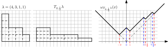
Figure 3. Young diagram $\lambda=(4,3,1,1)$ (left) and the anisotropic Young diagram $T_{2,\frac{1}{2}}\lambda$ (center) are in the French convention. The solid line in the rightmost picture is the profile $\omega_{T_{2,\frac{1}{2}}\lambda}$ of $T_{2,\frac{1}{2}}\lambda$, obtained by switching from the French to the Russian convention. The local minima $x_{1},x_{2},x_{3},x_{4}$ and maxima $y_{1},y_{2},y_{3}$ of the profile are indicated in red and blue, respectively.

Theorem 2.3 (Law of Large Numbers [DS19]).

Assume that $\chi_{d}\colon\mathbb{Y}_{d}\to\mathbb{R}$ are Jack characters such that $(\chi_{d})_{d\geq 1}$ fulfills the AFP. Let $\lambda_{d}$ be a random Young diagram with $d$ boxes distributed according to $\mathbb{P}^{(\alpha)}_{\chi_{d}}$, and let $\Lambda^{(\alpha)}_{d}$ be the associated rescaled diagram $\Lambda^{(\alpha)}$.

Then there exists some deterministic function $\omega_{\Lambda_{\infty}}\colon\mathbb{R}\to\mathbb{R}$ with the property that

(23) $$\lim_{d\to\infty}\omega_{\Lambda^{(\alpha)}_{d}}=\omega_{\Lambda_{\infty}},$$

where the convergence holds true with respect to the supremum norm, in probability.

Theorem 2.4 (Central Limit Theorem [DS19]).

Assume that $\chi_{d}\colon\mathbb{Y}_{d}\to\mathbb{R}$ are Jack characters such that $(\chi_{d})_{d\geq 1}$ fulfills the enhanced AFP. Consider the sequence of random functions

$${\Delta}^{(\alpha)}_{d}:=\sqrt{d}\cdot\frac{\omega_{\Lambda^{(\alpha)}_{d}}-\omega_{\Lambda_{\infty}}}{2}$$

and the observables

$$\langle\Delta^{(\alpha)}_{d},\,x^{\ell}\rangle:=\int_{\mathbb{R}}x^{\ell}\,\Delta^{(\alpha)}_{d}(x)dx,\quad\ell\in\mathbb{Z}_{\geq 1}.$$

Then the joint distribution of the random variables $\langle\Delta^{(\alpha)}_{d},\,x^{\ell}\rangle$, for $\ell=1,2,\cdots$, converges weakly to a (non-centered) Gaussian distribution.

In other terms, the sequence of random functions ${\Delta}^{(\alpha)}_{d}$ converges to some (non-centered) Gaussian random vector $\Delta_{\infty}$ valued in the space $(\mathbb{R}[x])^{\prime}$ of distributions, the dual space to polynomials, and the convergence holds in distribution as $d\to\infty$.

Informally, the LLN and CLT above describe the first and second order asymptotics of the profile $\omega_{\Lambda_{d}^{(\alpha)}}$ of a large random anisotropic partition:

$$\omega_{\Lambda_{d}^{(\alpha)}}=\omega_{\Lambda_{\infty}}+\frac{2}{\sqrt{d}}\cdot\Delta_{\infty}+o\left(\frac{1}{\sqrt{d}}\right)\!,\text{ as $d\to\infty$}.$$

2.6. Examples of characters with the AFP and the corresponding probability measures

2.6.1. Jack–Plancherel measure

Let

(24) $$\chi_{d}(\mu):=\begin{cases}1,&\text{if $\mu=(1^{d})$},\\ 0,&\text{otherwise},\end{cases}$$

be the normalized character of the regular representation of the symmetric group $\mathfrak{S}_{d}$. For $\alpha=1$, the associated probability measure $\mathbb{P}^{(\alpha=1)}_{\chi_{d}}$ is the celebrated Plancherel measure studied in [VK77, LS77, BDJ99, BOO00, Oko00, IO02]. For any $\alpha>0$, one can show (see [DS19]) that $\chi_{d}$ is a Jack character and the corresponding probability measure is the Jack–Plancherel measure with formula

$$\mathbb{P}^{{(\alpha)}}_{\chi_{d}}(\lambda)=\frac{\alpha^{d}\,d!}{j_{\lambda}^{(\alpha)}},$$

where

(25) $$j^{(\alpha)}_{\lambda}:=\prod_{(i,j)\in\lambda}\big{(}\alpha(\lambda_{i}-j)+(\lambda_{j}^{\prime}-i)+1\big{)}\big{(}\alpha(\lambda_{i}-j)+(\lambda_{j}^{\prime}-i)+\alpha\big{)},$$

and $\lambda^{\prime}=(\lambda^{\prime}_{1}\geq\lambda^{\prime}_{2}\geq\cdots)$ is the conjugate of the partition of $\lambda$, whose Young diagram (in French convention) is obtained from reflecting the Young diagram of $\lambda$ across the line $y=x$. The quantity $j^{(\alpha)}_{\lambda}$ originates from symmetric function theory, see e.g. Eq. 33 below.

Note that the cumulants associated to the Jack characters $\chi_{d}$ are given by

$$\kappa^{\chi_{d}}_{n}(k_{1},\dots,k_{n})=\begin{cases}1,&\text{when }n=1\text{ and }k_{1}=1,\\ 0,&\text{otherwise},\end{cases}$$

so the sequence $(\chi_{d})_{d\geq 1}$ has the enhanced AFP: indeed, all the constants in (19) and (21) vanish, i.e. $v_{k}=v_{k}^{\prime}=v_{(k|l)}=0$, for all $k,l\geq 2$. Hence, the theorems from Section 2.5, as well as our main theorems from Section 5, can be applied to this example, as long as the asymptotic condition (9) on $\alpha$ is satisfied. The regimes of high temperature ($g>0,\,\alpha=\Theta(d)$), low temperature ($g<0,\,\alpha=\Theta(d^{-1})$), and fixed temperature ($g=0,\,\alpha=\Theta(1)$) are all covered.

2.6.2. Jack–Schur–Weyl measure

Let $N\in\mathbb{R}$ be a real parameter and set

(26) $$\chi_{d}(\mu):=N^{-\|\mu\|},$$

For $N\in\mathbb{Z}_{\geq 1}$, this is the normalized $\mathfrak{S}_{d}$-character considered in Schur–Weyl’s construction, where $\mathfrak{S}_{d}$ acts naturally on $(\mathbb{C}^{N})^{\otimes d}=\mathbb{C}^{N}\otimes\cdots\otimes\mathbb{C}^{N}$. Using [Mac95, Ch. VI, (10.25)] for the value of the principal specialization of a Jack symmetric function, one finds:

(27) $$\mathbb{P}^{(\alpha)}_{\chi_{d}}(\lambda)=\frac{d!\,\sqrt{\alpha}^{\,d}}{N^{d}\cdot j^{(\alpha)}_{\lambda}}\cdot\prod_{(i,j)\in\lambda}\big{(}N\sqrt{\alpha}+(j-1)\alpha-(i-1)\big{)}.$$

For $\alpha=1$, the measure $\mathbb{P}^{(\alpha=1)}_{\chi_{d}}$ is the Schur–Weyl measure studied by Biane [Bia01], who proved the LLN for the corresponding large random Young diagrams and found an explicit formula for the limit shape. In addition, for any $\alpha>0$, the measure (27) becomes the Jack–Plancherel measure in the limit $N\to\infty$. Finally, the Jack–Schur–Weyl measure can be obtained as a limit of the $z$-measures $M^{(d)}_{z,z^{\prime},\theta}$ studied by Borodin and Olshanski, namely

$$\mathbb{P}^{(\alpha)}_{\chi_{d}}(\lambda)=\lim_{z^{\prime}\to\infty}M^{(d)}_{N\sqrt{\theta},z^{\prime},\theta}(\lambda),$$

holds with $\theta=\alpha^{-1}$ (see [BO05, Equation (1.1)]).

We remark that formula (27) defines a probability measure whenever $N\sqrt{\alpha}\in\mathbb{Z}_{\geq 1}\,$ or $\,-N/\sqrt{\alpha}\in\mathbb{Z}_{\geq 1}$; in these cases, each $\chi_{d}$ is a Jack character by definition. If $N\sqrt{\alpha}\in\mathbb{Z}_{\geq 1}$ (resp. $-N/\sqrt{\alpha}\in\mathbb{Z}_{\geq 1}$), then $\mathbb{P}^{{(\alpha)}}_{\chi_{d}}$ is supported on Young diagrams $\lambda\in\mathbb{Y}_{d}$ with $\ell(\lambda)\leq N\sqrt{\alpha}$ (resp. $\ell(\lambda^{\prime})\leq-N/\sqrt{\alpha}$).

The functions $\chi_{d}$ considered in this example are multiplicative, i.e. for $\mu^{1},\dots,\mu^{n}\in\mathbb{Y}_{\leq d}$ such that $\mu^{1}\cdots\mu^{n}\in\mathbb{Y}_{\leq d}$, one has $\chi_{d}(\mu^{1}\cdots\mu^{n})=\chi_{d}(\mu^{1})\cdots\chi_{d}(\mu^{n})$. Then all the cumulants $\kappa^{\chi_{d}}_{n}(k_{1},\dots,k_{n})$ of order $n\geq 2$ vanish, and in particular (19) is satisfied with all $v_{(k|l)}=0$; then $(\chi_{d})_{d\geq 1}$ has the enhanced AFP if (21) holds. As a result, all theorems from Section 2.5 and Section 5 can be applied if each $\chi_{d}$ is a Jack character, and if (9) and (21) are satisfied. We discuss all three possible regimes:

$\bullet$ High temperature: Let $g,c>0$, and $w,g^{\prime}\in\mathbb{R}$ be arbitrary parameters. Find sequences $\alpha=\alpha(d)>0,\ N=N(d)\in\frac{1}{\sqrt{\alpha}}\cdot\mathbb{Z}_{\geq 1}$ such that

$$N\sqrt{\alpha}=\frac{\sqrt{\alpha d}}{c}+w\sqrt{\alpha}+o(\sqrt{d}),\qquad\sqrt{\alpha}=g\sqrt{d}+g^{\prime}+o(1),\ \text{ as }d\to\infty.$$

This is possible by first choosing $\alpha$ satisfying the second condition, and then choosing a positive integer $N\sqrt{\alpha}$ satisfying the first condition; the latter amounts to choosing an integer in an interval of length $o(\sqrt{d})$, which is always feasible for large $d$. With these conditions on $\alpha,N$, the asymptotic relation (9) holds, and moreover

$$\chi_{d}(k)\ d^{\frac{k-1}{2}}=c^{k-1}-(k-1)wc^{k}\cdot d^{-\frac{1}{2}}+o(d^{-\frac{1}{2}}),$$

so (21) holds too, with $v_{k}=c^{k-1},\,v_{k}^{\prime}=-(k-1)wc^{k}$.

$\bullet$ Low temperature: Let $g,c<0$, and $w,g^{\prime}\in\mathbb{R}$ be arbitrary parameters. Find sequences $\alpha=\alpha(d)>0,\ N=N(d)\in-\sqrt{\alpha}\cdot\mathbb{Z}_{\geq 1}$ such that

$$-\frac{N}{\sqrt{\alpha}}=-\frac{\sqrt{d}}{c\sqrt{\alpha}}-\frac{w}{\sqrt{\alpha}}+o(\sqrt{d}),\qquad\frac{1}{\sqrt{\alpha}}=-g\sqrt{d}-g^{\prime}+o(1),\ \text{ as }d\to\infty.$$

With these asymptotics on $\alpha,N$, both (9) and (21) hold with $v_{k}=c^{k-1},\,v_{k}^{\prime}=-(k-1)wc^{k}$.

$\bullet$ Fixed temperature: In this regime, we would like $\alpha(d)=\alpha>0$ to be fixed. Set $g=0,\,g^{\prime}=\sqrt{\alpha}-\frac{1}{\sqrt{\alpha}}$, so that (9) holds. Let $c>0,\,w\in\mathbb{R}$ be arbitrary parameters.

The enhanced AFP property requires finding $N=N(d)\in\mathbb{R}$ such that either $N\sqrt{\alpha}\in\mathbb{Z}_{\geq 1},\ N\sqrt{\alpha}=\frac{\sqrt{\alpha d}}{c}+w\sqrt{\alpha}+o(1)$, or $-\frac{N}{\sqrt{\alpha}}\in\mathbb{Z}_{\geq 1},\ -\frac{N}{\sqrt{\alpha}}=-\frac{\sqrt{d}}{c\sqrt{\alpha}}-\frac{w}{\sqrt{\alpha}}+o(1)$. However, it is impossible to choose an integer in an interval of length $o(1)$. Nevertheless, we can pick $N,\alpha$ s.t. $N\sqrt{\alpha}\in\mathbb{Z}_{\geq 1},\ N\sqrt{\alpha}=\frac{\sqrt{\alpha d}}{c}+O(1)$, or $-\frac{N}{\sqrt{\alpha}}\in\mathbb{Z}_{\geq 1},\ -\frac{N}{\sqrt{\alpha}}=-\frac{\sqrt{d}}{c\sqrt{\alpha}}+O(1)$, which guarantees that the AFP condition is satisfied with $v_{k}=c^{k-1}$. The LLN from Theorem 5.1 only requires the AFP, so we can apply it to our example. The $c$–dependent limit shape was found by Biane [Bia01] in the special case $\alpha=1$; it coincides with the celebrated Vershik–Kerov/Logan–Shepp limit shape in the limit $c\to 0$.

Moreover, the proof of Theorem 5.2 shows that the weaker conditions imposed by the AFP guarantee that the cumulants of order $\geq 3$ vanish for the random variables $\langle\Delta^{(\alpha)}_{d},x^{m}\rangle$, and the limits $\lim_{d\to\infty}{\operatorname{Cov}(\langle\Delta^{(\alpha)}_{d},x^{k-2}\rangle,\,\langle\Delta^{(\alpha)}_{d},x^{l-2}\rangle)}$ exist and have explicit combinatorial formulas. The difference between the AFP and the enhanced AFP only affects the existence of the limit $\lim_{d\to\infty}{\mathbb{E}[\langle\Delta^{(\alpha)}_{d},x^{m}\rangle]}$, which is not guaranteed by the weaker assumption of the AFP. Note that the special case $\alpha=1$ discussed in [Śni06] omits this problem by proving the CLT for the centered observables (see [Śni06, Corollary 3.3]). Our case of a general fixed $\alpha>0$ covers this theorem, but we also prove a stronger result: our choice of $N,\alpha$, e.g. satisfying $N\sqrt{\alpha}\in\mathbb{Z}_{\geq 1},\ N\sqrt{\alpha}=\sqrt{\alpha d}/c+O(1)$, implies that we can restrict to a subsequence $(d_{k})_{k}$ such that $N(d_{k})\sqrt{\alpha(d_{k})}=\sqrt{\alpha(d_{k})d_{k}}/c+w\sqrt{\alpha(d_{k})}+o(1)$, for some fixed $w\in\mathbb{R}$. Then the convergence of the random function $\Delta^{(\alpha)}_{d}$ to the Gaussian process $\Delta_{\infty}$ stated in Theorem 5.2 still holds true but with the sequence $(\Delta^{(\alpha)}_{d})_{d\in\mathbb{Z}_{\geq 1}}$ replaced by $(\Delta^{(\alpha)}_{d_{k}})_{k\in\mathbb{Z}_{\geq 1}}$.

2.6.3. Conditional Plancherel-type Jack measure

Let $(v_{k})_{k\geq 2}$ be any sequence of reals satisfying (20), and for any integer $k\geq 2$, choose a sequence $(v^{(d)}_{k})_{d\geq 1}$ such that

(28) $$v^{(d)}_{k}\cdot d^{\frac{k-1}{2}}=v_{k}+o(d^{-\frac{1}{2}}),\text{ as }d\to\infty.$$

Then consider the following function on $\mathbb{Y}_{d}$:

$$\chi_{d}(\mu):=\prod_{{k}\geq 2}\left(v^{(d)}_{{k}}\right)^{m_{k}(\mu)}.$$

These functions are multiplicative; together with (28), we conclude that $(\chi_{d})_{d\geq 1}$ satisfies the enhanced AFP with $v_{k}^{\prime}=v_{(k|l)}=0$. We prove in Proposition 5.3 that the associated measure can be expressed as

$$\mathbb{P}^{(\alpha)}_{\chi_{d}}(\lambda)=\frac{\alpha^{d}\,d!}{u^{d}}\cdot\frac{J_{\lambda}^{(\alpha)}(u\cdot\mathbf{v}_{u,\alpha})}{j^{(\alpha)}_{\lambda}},$$

where $u>0$ is arbitrary, and $J_{\lambda}^{(\alpha)}(u\cdot\mathbf{v}_{u,\alpha})$ is defined as the image of $J_{\lambda}^{(\alpha)}$ under the specialization (unital algebra homomorphism) $\rho\colon\operatorname{Sym}\rightarrow\mathbb{C}$ from the $\mathbb{R}$-algebra of symmetric functions $\operatorname{Sym}$ that maps the power sums $p_{k}\,$ to $\,u\cdot(u/\sqrt{\alpha})^{k-1}\cdot v_{k}^{(d)}$.

In order to apply our main results, including those from Section 5, we must impose that $\alpha$ satisfies (9) and that each $\chi_{d}$ is a Jack character. One contribution of this paper is the classification of the totally Jack positive specializations in Theorem 4.4 that allows to find large families of examples of parameters $\alpha,\,v_{k}^{(d)}$ that fit into this setting. By Proposition 4.6 and Proposition 5.3, we are able to consider all three limit regimes as follows.

$\bullet$ High temperature: Consider any parameters $g>0$ and $a_{1}\geq a_{2}\geq\cdots\geq 0$ such that $\sum_{i=1}^{\infty}{a_{i}}\leq 1$. Set $\alpha=g^{2}d$, so that (9) holds with $g^{\prime}=0$. Also set

(29) $$v_{k}^{(d)}=\left(\frac{g\sqrt{d}}{\lceil gd\rceil}\right)^{k-1}\cdot\sum_{i=1}^{\infty}{a_{i}^{k}},\ \text{ for }k\geq 2.$$

Then $(\chi_{d})_{d\geq 1}$ are Jack characters with the enhanced AFP and $v_{k}=\!\sum_{i=1}^{\infty}{a_{i}^{k}}$.

$\bullet$ Low temperature: Consider any parameters $g<0$ and $a_{1}\geq a_{2}\geq\cdots\geq 0$ such that $\sum_{i=1}^{\infty}{a_{i}}\leq 1$. Set $\alpha=\frac{1}{(-g)\cdot\lceil-gd\rceil}$, so that (9) holds with $g^{\prime}=0$. Also set

(30) $$v_{k}^{(d)}=\left(\frac{-\sqrt{-g}}{\sqrt{\lceil-gd\rceil}}\right)^{k-1}\cdot\sum_{i=1}^{\infty}a_{i}^{k},\ \text{ for }k\geq 2.$$

Then $(\chi_{d})_{d\geq 1}$ are Jack characters with the enhanced AFP and $v_{k}=(-1)^{k-1}\sum_{i=1}^{\infty}{a_{i}^{k}}$.

$\bullet$ Fixed temperature: For this regime, $\alpha>0$ is fixed, so $g=0,\,g^{\prime}=\sqrt{\alpha}-\frac{1}{\sqrt{\alpha}}$. We prove in Proposition 5.3 that $\chi_{d}$ is a Jack character whenever $(\sqrt{\alpha},\sqrt{\alpha}\,v_{2}^{(d)},\sqrt{\alpha}\,v_{3}^{(d)},\dots)$ determines an $\alpha$-Jack-positive specialization, as in Definition 4.1. Then Theorem 4.2, due to Kerov–Okounkov–Olshanski [KOO98], characterizes the valid sequences $(v_{k}^{(d)})_{k}$. Take for instance any reals $a_{1}\geq a_{2}\geq\dots\geq 0$ and $b_{1}\geq b_{2}\geq\dots\geq 0$ such that $\sum_{i=1}^{\infty}(a_{i}+b_{i})\leq 1$, and a sequence of integers $n=n(d)$ such that $n\leq\sqrt{\alpha d}$ and $n=\sqrt{\alpha d}+O(1)$; then set:

$$v_{k}^{(d)}:=\frac{n}{\sqrt{\alpha}}\cdot\sum_{i=1}^{\infty}\left(\frac{a_{i}}{\sqrt{d}}\right)^{k}+\frac{n}{\sqrt{\alpha}}\cdot(-\alpha)^{1-k}\sum_{i=1}^{\infty}\left(\frac{b_{i}}{\sqrt{d}}\right)^{k},\ \text{ for }k\geq 2.$$

Then all results from Section 5 hold true, except for the existence of the limits $\lim_{d\to\infty}{\mathbb{E}[\langle\Delta^{(\alpha)}_{d},x^{m}\rangle]}$; for that, one must restrict to subsequences $(d_{k})_{k}$ with $n(d_{k})=\sqrt{\alpha(d_{k})d_{k}}+o(1)$, cf. Section 2.6.2 and Remark 5. The parameters $v_{k}$ are $v_{k}=\sum_{i=1}^{\infty}{a_{i}^{k}}+(-\alpha)^{1-k}\sum_{i=1}^{\infty}{b_{i}^{k}}$.

Remark 4.

We point out that the scaling of the random partitions in our LLN is different from that in [KOO98, Ver74]. Indeed, these other articles discuss a LLN in which the parameters $a_{1},a_{2},\cdots$ (resp. $b_{1},b_{2},\cdots$) appear as the rates of linear growth of rows (reps. columns) of the random partitions. In contrast, our random partitions $\lambda^{(d)}\in\mathbb{Y}_{d}$ are balanced in the sense that both the number of rows and columns are asymptotically proportional to $\sqrt{d}$.

Remark 5.

In general, whenever we replace the assumption of the enhanced AFP by the (weaker) AFP in Theorem 5.2, we have its weaker version which says that the family of centered random variables $x_{\ell}:=X_{\ell}-\mathbb{E}X_{\ell}$, where $X_{\ell}:=\langle\Delta^{(\alpha)}_{d},x^{\ell}\rangle$, converges jointly to a Gaussian distribution in the weak topology of probability measures. The special case $\alpha=1$ recovers the result of Śniady [Śni06]. Similarly, by replacing (21) in the definition of the enhanced AFP by a weaker condition $\chi_{d}(k)\ d^{\frac{k-1}{2}}=v_{k}+O(d^{-\frac{1}{2}})$ that we encountered in all our examples, then Theorem 5.2 holds true after restricting to a subsequence.

3. Second model of random Young diagrams: Jack measures

In this section, we review the construction from [Mol23] that yields probability measures on the infinite set $\mathbb{Y}:=\bigsqcup_{d\geq 0}\mathbb{Y}_{d}$ of all Young diagrams and it relies on the Cauchy identity for Jack symmetric functions; the result is a natural $1$-parameter generalization of Okounkov’s Schur measures [Oko01]. We also isolate a special family of Jack measures, called Plancherel-type Jack measures, that are closely related to the model of random Young diagrams discusssed in Section 2, and to the work of Kerov-Okounkov-Olshanski [KOO98]. We prove the LLN and CLT for this new family of measures.

3.1. Definitions and preliminaries

Recall the Cauchy identity for Jack symmetric functions [Mac95, Ch. VI.10]:

(31) $$1+\sum_{d=1}^{\infty}{t^{d}\sum_{\lambda\in\mathbb{Y}_{d}}{\frac{J_{\lambda}^{(\alpha)}(\mathbf{p})J_{\lambda}^{(\alpha)}(\mathbf{q})}{\|J_{\lambda}^{(\alpha)}\|^{2}}}}=1+\sum_{d=1}^{\infty}{t^{d}\sum_{\mu\in\mathbb{Y}_{d}}{\frac{p_{\mu}q_{\mu}}{\alpha^{\ell(\mu)}z_{\mu}}}}=\exp\bigg{(}\sum_{k\geq 1}\frac{t^{k}p_{k}q_{k}}{{k}\alpha}\bigg{)},$$

where $\mathbf{p}=(p_{1},p_{2},\dots)$ and $\mathbf{q}=(q_{1},q_{2},\dots)$ are two independent families of variables which play the role of power-sums. We employed the usual notations: $p_{\mu}:=\prod_{i\geq 1}{p_{\mu_{i}}}$, $J_{\lambda}(\mathbf{p}):=\sum_{\mu\in\mathbb{Y}_{d}}\theta^{(\alpha)}_{\mu}(\lambda)p_{\mu}$, and $q_{\mu},J_{\lambda}(\mathbf{q})$ are defined similarly.The norm $\|\cdot\|$ in the LHS of (31) is with respect to the $\alpha$-deformed Hall scalar product, defined on the $\mathbb{R}$-algebra of symmetric functions $\operatorname{Sym}$ by declaring the basis $\{p_{\mu}\}_{\mu\in\mathbb{Y}}$ to be orthogonal, and

(32) $$\|p_{\mu}\|^{2}=\alpha^{\ell(\mu)}z_{\mu},\quad\forall\,\mu\in\mathbb{Y}.$$

It is known that the Jack symmetric functions $J^{(\alpha)}_{\lambda}$ are orthogonal and have norms

(33) $$\|J^{(\alpha)}_{\lambda}\|^{2}=j^{(\alpha)}_{\lambda},$$

where $j^{(\alpha)}_{\lambda}$ is given in (25). Note that $j^{{(\alpha)}}_{\lambda}\in\mathbb{Z}_{\geq 0}[\alpha]$, in particular $j^{(\alpha)}_{\lambda}>0$, whenever $\alpha>0$.

Definition 3.1 (Second model of random Young diagrams: Jack measures).

Given a fixed $\alpha>0$, let $\rho_{1},~{}\rho_{2}:\operatorname{Sym}\to\mathbb{C}$ be any two unital $\mathbb{R}$-algebra homomorphisms such that

(34) $$\rho_{1}\left(J_{\lambda}^{(\alpha)}\right)\overline{\rho_{2}\left(J_{\lambda}^{(\alpha)}\right)} \geq 0,\text{ for all }\lambda\in\mathbb{Y},$$

(35) $$\sum_{k=1}^{\infty}{\frac{\rho_{1}(p_{k})\overline{\rho_{2}(p_{k})}}{k}} <\infty.$$

Then define the Jack measure $M^{(\alpha)}_{\rho_{1},\rho_{2}}$ as the probability measure on $\mathbb{Y}$ given by

(36) $$M_{\rho_{1},\rho_{2}}^{(\alpha)}(\lambda):=\frac{\rho_{1}\left(J_{\lambda}^{(\alpha)}\right)\overline{\rho_{2}\left(J_{\lambda}^{(\alpha)}\right)}}{j^{(\alpha)}_{\lambda}}\exp\left(-\sum_{k=1}^{\infty}{\frac{\rho_{1}(p_{k})\overline{\rho_{2}(p_{k})}}{k\alpha}}\right),\quad\lambda\in\mathbb{Y}.$$

The normalization $\,\sum_{\lambda\in\mathbb{Y}}{M^{(\alpha)}_{\rho_{1},\rho_{2}}(\lambda)}=1$ follows from (31), while the nonnegativity $M^{(\alpha)}_{\rho_{1},\rho_{2}}(\lambda)\geq 0$ is a direct consequence of the assumptions (34), (35).

3.2. Examples of Jack measures

3.2.1. Principal series Jack measures

The measure $M_{\rho_{1},\rho_{2}}^{(\alpha)}$ was studied by the third author in the special case when $\rho:=\rho_{1}=\rho_{2}$, see [Mol23]. Note that (34) is automatically satisfied when the specializations $\rho_{1},\rho_{2}$ are equal. The main results of [Mol23] are the LLN and CLT for $M_{\rho,\rho}^{(\alpha)}$ under certain technical assumptions on $\rho$ (which in particular guarantee (35)), namely $|\rho(p_{k})|\leq A\cdot r^{k}$, for all ${k}\geq{1}$, and some constants $A>0,\,r<1$.

3.2.2. Poissonized Jack–Plancherel measures

Let us look at the special case of Section 3.2.1 when $\rho(p_{k})=u\cdot\delta_{1,{k}}$, for some $u\in\mathbb{C}$, and $\delta_{1,k}$ is the Kronecker delta. This is the so-called Plancherel specialization. From the fact that the coefficient of $p_{1}^{|\lambda|}$ in the expansion of $J^{{(\alpha)}}_{\lambda}$ is $1$ (see [Mac95, Ch. VI, (10.29)]), one finds the explicit formula

$$M_{\rho,\rho}^{(\alpha)}(\lambda)=\exp\left(-\frac{|u|^{2}}{\alpha}\right)\frac{|u|^{2|\lambda|}}{j^{(\alpha)}_{\lambda}}.$$

Observe that $M_{\rho,\rho}^{(\alpha)}$ is the Poissonization of the Jack–Plancherel measures from Section 2.6.1 with the Poisson parameter equal to $\frac{|u|^{2}}{\alpha}$. In other words,

$$M_{\rho,\rho}^{{(\alpha)}}(\lambda)=\exp\left(-\frac{|u|^{2}}{\alpha}\right)\frac{|u|^{2d}}{\alpha^{d}d!}\cdot\mathbb{P}_{\chi_{d}}^{(\alpha)}(\lambda),\quad\forall\,\lambda\in\mathbb{Y}_{d},\ d\in\mathbb{Z}_{\geq 0},$$

where $\mathbb{P}_{\chi_{d}}^{{(\alpha)}}$ is the probability measure associated with the character $\chi_{d}$ from Section 2.6.1.

3.2.3. Poissonized Jack–Schur–Weyl measures

Consider a generalization of the previous example, when $\rho_{1}$ is the principal specialization $\rho_{1}(p_{k})=u\cdot c^{k-1}$, while $\rho_{2}$ is still the Plancherel specialization $\rho_{2}(p_{k})=u\cdot\delta_{1,k}$. This example is not an instance of Section 3.2.1, but it clearly satisfies (35). One can also check that (34) is satisfied whenever $u\in\mathbb{R},c\in\mathbb{R}^{*}$, and $u/c\in\mathbb{Z}_{\geq 1}$ or $-u/(c\alpha)\in\mathbb{Z}_{\geq 1}$. Indeed, by [Mac95, Ch. VI, (10.25)], one finds

$$M_{\rho_{1},\rho_{2}}^{(\alpha)}(\lambda)=\exp\left(-\frac{u^{2}}{\alpha}\right)\cdot\frac{(uc)^{|\lambda|}}{j_{\lambda}^{(\alpha)}}\cdot\prod_{(i,j)\in\lambda}{\left(\frac{u}{c}+\alpha(j-1)-(i-1)\right)}.$$

If $u/c\in\mathbb{Z}_{\geq 1}$ (resp. $-u/(c\alpha)\in\mathbb{Z}_{\geq 1}$), then $M_{\rho_{1},\rho_{2}}^{(\alpha)}$ is supported on partitions $\lambda$ with $\ell(\lambda)\leq u/c$ (resp. $\ell(\lambda^{\prime})\leq-u/(c\alpha)$). Moreover, $M_{\rho_{1},\rho_{2}}^{(\alpha)}$ is the Poissonization of the Jack–Schur–Weyl measures $\mathbb{P}_{\chi_{d}}^{{(\alpha)}}$ from Section 2.6.2 with $N=\frac{u}{c\sqrt{\alpha}}$ and Poisson parameter $\frac{u^{2}}{\alpha}$.

3.2.4. Plancherel-type Jack measures

The example from Section 3.2.3 is a special case of the following general framework that will be the main object of interest later in this section. Let $\mathbf{v}=(v_{1},v_{2},\cdots)\in\mathbb{R}^{\infty}$ and $u>0$. Define $M^{(\alpha)}_{u;\mathbf{v}}$ as the Jack measure $M_{\rho_{1},\rho_{2}}^{{(\alpha)}}$ with specializations $\rho_{1}(p_{k})=u\cdot v_{k}$ and $\rho_{2}(p_{k})=u\cdot\delta_{1,{k}}$. If we denote $u\cdot\mathbf{v}:=(u\cdot v_{1},u\cdot v_{2},\cdots)$ and $J_{\lambda}^{(\alpha)}(u\cdot\mathbf{v}):=\rho(J_{\lambda}^{(\alpha)})$, for the specialization $\rho(p_{k}):=u\cdot v_{k}$, then

$$M^{(\alpha)}_{u;\mathbf{v}}(\lambda)=\exp\left(-\frac{u^{2}\cdot v_{1}}{\alpha}\right)\frac{J_{\lambda}^{(\alpha)}(u\cdot\mathbf{v})\cdot u^{|\lambda|}}{j^{(\alpha)}_{\lambda}}.$$

This is a probability measure if and only if $J_{\lambda}^{(\alpha)}(u\cdot\mathbf{v})\geq 0$, for all $\lambda\in\mathbb{Y}$. We find in Section 4 some choices of $u,\mathbf{v}$ that imply this positivity assumption, see e.g. Proposition 4.6. We shall refer to $M^{(\alpha)}_{u;\mathbf{v}}$ as a Plancherel-type Jack measure. We prove in Proposition 5.3 that if $v_{1}=1$, the measure $M^{(\alpha)}_{u;\mathbf{v}}$ is the Poissonization of the measures $\mathbb{P}_{\chi_{d}}^{{(\alpha)}}$ from Section 2.6.3 with Poisson parameter $\frac{u^{2}}{\alpha}$.

3.3. Transition measure and observables of measures

Given any Young diagram $\lambda\in\mathbb{Y}$, we use Kerov’s idea [Ker93] to associate to $\lambda$ a probability measure $\mu_{\lambda}$ on $\mathbb{R}$, called the transition measure; it is characterized by the following identity for its Cauchy transform:

(37) $$G_{\mu_{\lambda}}(z)=\int_{\mathbb{R}}\frac{d\mu_{\lambda}(x)}{z-x}=\frac{1}{z+\ell(\lambda)}\prod_{i=1}^{\ell(\lambda)}\frac{z+i-\lambda_{i}}{z+i-1-\lambda_{i}}=\frac{\prod_{i=1}^{k}(z-y_{i})}{\prod_{i=1}^{k+1}(z-x_{i})},$$

where $x_{1},\dots,x_{k+1}$ ($y_{1},\dots,y_{k}$, respectively) are the local minima (maxima, respectively) of the profile $\omega_{\lambda}$, see Fig. 3. More generally, we can define the transition measure $\mu_{T_{w,h}\lambda}$ of any anisotropic diagram $T_{w,h}\lambda$ by the same equation (37). Note that the mean of any transition measure is $\int_{\mathbb{R}}{x\,d\mu_{T_{w,h}\lambda}(x)}=\sum_{i=1}^{k+1}{x_{i}}-\sum_{i=1}^{k}{y_{i}}=0$.

Below we will use various sequences of observables on the space of probability measures on $\mathbb{R}$ with finite moments of all orders. Besides the moments, we will use the Boolean cumulants, the free cumulants and the fundamental functionals of shape. If $\mu$ is a probability measure on $\mathbb{R}$ with finite moments of all orders, then let us denote its $\ell$-th moment by $M^{\mu}_{\ell}:=\int_{\mathbb{R}}{x^{\ell}\mu(dx)}$. The sequence of moments $(M^{\mu}_{\ell})_{\ell\geq 1}$ can also be described by expanding the Cauchy transform of $\mu$ in a neighborhood of infinity:

(38) $$G_{\mu}(z)=\int_{\mathbb{R}}\frac{d\mu(x)}{z-x}=\frac{1}{z}+\sum_{\ell\geq 1}M^{\mu}_{\ell}z^{-\ell-1}.$$

The associated sequences of Boolean cumulants $(B^{\mu}_{\ell})_{\ell\geq 1}$, free cumulants $(R^{\mu}_{\ell})_{\ell\geq 1}$, and fundamental functionals of shape $(S^{\mu}_{\ell})_{\ell\geq 1}$ can be defined by the following relations between their generating functions:

(39) $$B_{\mu}(z) :=\sum_{\ell\geq 1}B^{\mu}_{\ell}\,z^{-\ell+1}=z-\frac{1}{G_{\mu}(z)},$$

(40) $$K_{\mu}(z) :=\sum_{\ell\geq 1}R^{\mu}_{\ell}\,z^{\ell-1}=G^{-1}_{\mu}(z)-\frac{1}{z},$$

(41) $$S_{\mu}(z) :=\sum_{\ell\geq 1}S^{\mu}_{\ell}\,z^{-\ell}=\log\left(zG_{\mu}(z)\right),$$

where $G^{-1}_{\mu}(z)$ denotes the (formal) compositional inverse of $G_{\mu}$. Observe that the first elements in these sequences of observables are the same: $B^{\mu}_{1}=R^{\mu}_{1}=S^{\mu}_{1}=M^{\mu}_{1}$.

Proposition 3.2.

For any integer $\ell\geq 1$,

(42) $$M^{\mu}_{\ell} =\sum_{n\geq 1}\sum_{k_{1},\dots,k_{n}\geq 1\atop k_{1}+\cdots k_{n}=\ell}B^{\mu}_{k_{1}}\cdots B^{\mu}_{k_{n}},$$

(43) $$S^{\mu}_{\ell} =\sum_{n\geq 1}\frac{1}{n}\sum_{k_{1},\dots,k_{n}\geq 1\atop k_{1}+\cdots k_{n}=\ell}B^{\mu}_{k_{1}}\cdots B^{\mu}_{k_{n}}.$$

Proof.

In order to prove (42), we use (39):

$$M^{\mu}_{\ell}=[z^{-\ell-1}]G_{\mu}(z)=[z^{-\ell-1}]\frac{1}{z-B_{\mu}(z)}=[z^{-\ell}]\frac{1}{1-z^{-1}B_{\mu}(z)}=[z^{-\ell}]\sum_{n\geq 1}(z^{-1}B_{\mu}(z))^{n},$$

which equals the right hand side of (42). Similarly, to prove (43), we use (39) and (41) to get

$$S^{\mu}_{\ell}=[z^{-\ell}]\log\left(zG_{\mu}(z)\right)=[z^{-\ell}]\log\bigg{(}\frac{1}{1-z^{-1}B_{\mu}(z)}\bigg{)}=[z^{-\ell}]\sum_{n\geq 1}{\frac{1}{n}(z^{-1}B_{\mu}(z))^{n}},$$

which equals the right hand side of (43). ∎

The moments, Boolean cumulants, free cumulants and fundamental functionals of shape associated with the transition measure $\mu_{\lambda}$ will be denoted by $M_{\ell}(\lambda)$, $B_{\ell}(\lambda)$, $R_{\ell}(\lambda)$, $S_{\ell}(\lambda)$, respectively, and we think of them as functions on the set of Young diagrams. We will also use the analogous notations if the Young diagram $\lambda$ is replaced by an anisotropic diagram.

Finally, we remark that for all $X=M,B,R,S$, we have $X_{1}(T_{w,h}\lambda)=0$, for all anisotropic diagrams $T_{w,h}\lambda$, as well as the following scaling property $X_{\ell}(T_{cw,ch}\lambda)=c^{\ell}X_{\ell}(T_{w,h}\lambda)$, in particular:

(44) $$X_{\ell}(\Lambda_{(\alpha;u)})=u^{-\ell}X_{\ell}(\Lambda_{(\alpha;1)}).$$

3.4. The Markov–Krein correspondence

The relation between the profile $\omega_{\Lambda}$ and the transition measure $\mu_{\Lambda}$ of an anisotropic diagram $\Lambda$ is given by (37) and this can be restated in the following form, known as the Markov–Krein correspondence:

(45) $$\frac{1}{z}\exp\int_{\mathbb{R}}\frac{1}{x-z}\left(\frac{\omega_{\Lambda}(x)-|x|}{2}\right)^{\prime}dx=\int_{\mathbb{R}}\frac{d\mu_{\Lambda}(x)}{z-x}.$$

Applying (41) to the above equation, we obtain the following formula for the fundamental functional of shape:

(46) $$S_{n}(\Lambda)=-\int_{\mathbb{R}}x^{n-1}\left(\frac{\omega_{\Lambda}(x)-|x|}{2}\right)^{\prime}dx=(n-1)\int_{\mathbb{R}}x^{n-2}\left(\frac{\omega_{\Lambda}(x)-|x|}{2}\right)dx.$$

The Markov–Krein correspondence works in a much wider generality, and we briefly state it here in the most general framework that we are aware of.

We call generalized continuous Young diagram a continuous function $\omega\colon\mathbb{R}\to\mathbb{R}$ with Lipschitz constant $1$ and such that the following integrals converge:

(47) $$\int_{-\infty}^{0}\frac{1+\omega^{\prime}(x)}{1-x}dx<\infty;\ \ \ \ \int_{0}^{\infty}\frac{1-\omega^{\prime}(x)}{1+x}dx<\infty.$$

We denote by $\mathbb{Y}^{1}$ the set of equivalence classes of generalized continuous Young diagrams, where $\omega_{1}\sim\omega_{2}\iff\omega_{1}^{\prime}\equiv\omega_{2}^{\prime}$. The space of generalized continuous Young diagrams $\mathbb{Y}^{1}$ is a Polish space (separable and metrizable complete space) with the following topology: we say that $\omega_{n}\to\omega$ if the following integrals are uniformly bounded:

$$\sup_{n\in\mathbb{Z}_{\geq 0}}\left(\int_{-\infty}^{0}\frac{1+\omega_{n}^{\prime}(x)}{1-x}dx\right)<\infty;\ \ \ \ \sup_{n\in\mathbb{Z}_{\geq 0}}\left(\int_{0}^{\infty}\frac{1-\omega_{n}^{\prime}(x)}{1+x}dx\right)<\infty,$$

and there exist representatives $\omega_{n}(x)$ and $\omega(x)$ such that for any $N>0$ one has $\lim_{n\to\infty}\|\omega_{n}-\omega\|_{L^{\infty}([-N,N])}=0$.

We define two other Polish spaces (see [M1́7] for the details): $\mathscr{M}^{1}$ the space of probability measures on the real line $\mathbb{R}$ with the topology of weak convergence and $\mathscr{N}^{1}$ the space of holomorphic functions $h$ on the Poincáre half-space

$$\mathbb{H}:=\{z\in\mathbb{C}\colon\Im(z)>0\}$$

which take values with negative imaginary parts and such that $\lim_{y\to+\infty}\mathbf{i}yh(\mathbf{i}y)=1$ if $\mathbf{i}=\sqrt{-1}$ (the topology is given by the proper convergence i.e. $h_{n}\to h$ if $h_{n}$ converges uniformly to $h$ on all compact subsets of $\mathbb{H}$ and

$$\lim_{N\to\infty}\sup_{n\in\mathbb{Z}_{\geq 0}\atop y\geq N}|\mathbf{i}yh_{n}(\mathbf{i}y)-1|=0).$$

Then, the following Markov–Krein correspondence holds true.

Theorem 3.3.

[M1́7, Theorem 7.25] There is a sequence of homeomorphisms

$$\omega\in\mathbb{Y}^{1}\leftrightarrow G_{\omega}\in\mathscr{N}^{1}\leftrightarrow\mu_{\omega}\in\mathscr{M}^{1}$$

given by:

(48) $$G_{\omega}(z)=\int_{\mathbb{R}}\frac{d\mu_{\omega}(x)}{z-x}=\frac{1}{z}\exp\int_{\mathbb{R}}\frac{1}{x-z}\left(\frac{\omega(x)-|x|}{2}\right)^{\prime}dx.$$

Similarly as before, we will study the typical shape of the rescaled diagram $\Lambda_{(\alpha;u)}$ given by (22) when $\lambda$ is sampled from the Plancherel-type Jack measure $M^{(\alpha)}_{(u;\mathbf{v})}$, and the Poisson parameter tend to infinity. We prove that in various regimes such a typical shape $\Lambda_{(\mathbf{v},g)}$ exists, the fluctuations around this shape are Gaussian and we describe it via the Markov–Krein correspondence (we give an explicit combinatorial formula for the associated Cauchy transform $G_{\omega_{\Lambda_{(\mathbf{v},g)}}}(z)$ in terms of lattice paths).

3.5. Łukasiewicz paths and Łukasiewicz ribbon paths

An excursion $\Gamma$ of length $\ell$ is a sequence of points $\Gamma=(w_{0},\dots,w_{\ell})$ on $(\mathbb{Z}_{\geq 0})^{2}$ such that $w_{j}=(j,y_{j})$, with $y_{0}=y_{\ell}=0$, $y_{1},\dots,y_{\ell-1}\in\mathbb{Z}_{\geq 0}$, and it is uniquely encoded by the sequence of its steps $e_{j}:=w_{j}-w_{j-1}=(1,y_{j}-y_{j-1})$. Informally speaking, an excursion is a directed lattice path with steps of the form $(1,k),k\in\mathbb{Z}$, starting at $(0,0)$, finishing at $(\ell,0)$, and that stays in the first quadrant. A step $e=(1,0)$ is called a horizontal step, while steps $e=(1,k),\,k\in\mathbb{Z}_{>0}$ (resp. $k\in\mathbb{Z}_{<0}$), are called up steps (resp. down steps) of degree $k$, see Fig. 4 for examples.

For a given excursion $\Gamma=(w_{0},\dots,w_{\ell})$, the set of points $\mathbf{S}(\Gamma):=\{w_{1},w_{2},\dots,w_{\ell}\}$ (not counting the origin $w_{0}=(0,0)$) naturally decomposes into pairwise disjoint subsets consisting of those points which are preceded by a horizontal, down step or up step:

$$\mathbf{S}(\Gamma)=\mathbf{S}_{\tiny\rightarrow}(\Gamma)\cup\mathbf{S}_{\tiny\searrow}(\Gamma)\cup\mathbf{S}_{\tiny\nearrow}(\Gamma).$$

Denote by $\mathbf{S}_{n}(\Gamma)$, $n\in\mathbb{Z}\setminus\{0\}$, the set of points preceded by a step $(1,n)$, i.e. $\mathbf{S}_{n}(\Gamma)$ is the set of points preceded by an up step of degree $n$, if $n>0$, or by a down step of degree $-n$, if $n<0$. Also denote by $\mathbf{S}^{i}(\Gamma)$ the subset of points with second coordinate equal to $i$, i.e.

$$\mathbf{S}^{i}(\Gamma):=\{w_{j}=(j,y_{j})\in\mathbf{S}(\Gamma)\,\mid\,y_{j}=i\}.$$

We say that points $w_{j}\in\mathbf{S}^{i}(\Gamma)$ are at height $i$. The set $\mathbf{S}^{0}(\Gamma)$ will play an especially prominent role (e.g. see Theorem 3.8 below); note that the origin $w_{0}=(0,0)$ does not belong to $\mathbf{S}^{0}(\Gamma)$.

Define the sets $\mathbf{S}^{i}_{\tiny\rightarrow}(\Gamma),\mathbf{S}^{i}_{\tiny\searrow}(\Gamma),\mathbf{S}^{i}_{\tiny\nearrow}(\Gamma),\mathbf{S}^{i}_{n}(\Gamma)$, $n\in\mathbb{Z}\setminus\{0\}$, analogously.

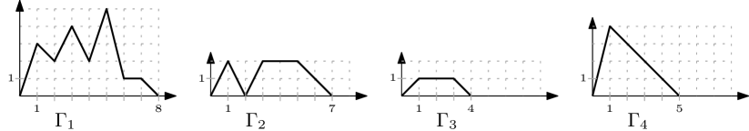
Figure 4. Four excursions $\Gamma_{1},\Gamma_{2},\Gamma_{3}$ and $\Gamma_{4}$. Note that $\Gamma_{3}$ and $\Gamma_{4}$ are Łukasiewicz paths, but $\Gamma_{1}$ and $\Gamma_{2}$ are not.

Summing up, we have the following natural decompositions into disjoint subsets:

$$\mathbf{S}(\Gamma)=\bigcup_{i=0}^{\infty}\,\Bigl{\{}\mathbf{S}^{i}_{\tiny\rightarrow}(\Gamma)\cup\mathbf{S}^{i}_{\tiny\searrow}(\Gamma)\cup\mathbf{S}^{i}_{\tiny\nearrow}(\Gamma)\Bigr{\}}=\bigcup_{i=0}^{\infty}\,\Bigl{\{}\mathbf{S}^{i}_{\tiny\rightarrow}(\Gamma)\cup\bigcup_{n=1}^{\infty}\bigl{(}\mathbf{S}^{i}_{-n}(\Gamma)\cup\mathbf{S}^{i}_{n}(\Gamma)\bigr{)}\Bigr{\}}.$$

For an ordered tuple $\vec{\Gamma}=(\Gamma_{1},\dots,\Gamma_{k})$ of $k$ excursions $\Gamma_{i}$, we will treat $\vec{\Gamma}$ itself as the excursion obtained by concatenating $\Gamma_{1},\dots,\Gamma_{k}$. We define $\mathbf{S}(\vec{\Gamma}),\mathbf{S}_{\tiny\rightarrow}^{i}(\vec{\Gamma}),\mathbf{S}_{n}^{i}(\vec{\Gamma})$, etc. in the same way as before, by treating $\vec{\Gamma}$ as the excursion obtained from the concatenation of $\Gamma_{1},\dots,\Gamma_{k}$. For example, if $\vec{\Gamma}=(w_{0},w_{1},\dots,w_{\ell})$, then $\mathbf{S}(\vec{\Gamma})=\{w_{1},\dots,w_{\ell}\}$. We say that $p=(w_{i},w_{j})$ is a pairing of degree $n>0$ if $w_{i}\in\mathbf{S}_{-n}(\vec{\Gamma}),w_{j}\in\mathbf{S}_{n}(\vec{\Gamma})$, and $w_{i}$ appears before $w_{j}$ in $\vec{\Gamma}$, i.e. $i<j$. See Fig. 4 and Fig. 5 for an example.

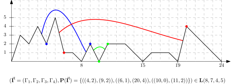
Figure 5. A ribbon path $\vec{\bm{\Gamma}}=(\Gamma_{1},\Gamma_{2},\Gamma_{3},\Gamma_{4})$ on $4$ sites of lengths $8,7,4,5$, which is also a Łukasiewicz ribbon path belonging to $\mathbf{L}(8,7,4,5)$. The three pairs of dots of different colors (red, green and blue) are examples of pairings, and the colored arcs join the pairs of preceding steps of the same degree. The degrees of the red, green and blue pairings are $4$, $2$ and $2$, respectively.

By definition, a ribbon path on $k$ sites of lengths $\ell_{1},\dots,\ell_{k}$ is a pair $\vec{\bm{\Gamma}}=(\vec{\Gamma},\,\mathbf{P}(\vec{\bm{\Gamma}}))$ consisting of an ordered tuple $\vec{\Gamma}$ of $k$ excursions $\Gamma_{1},\dots,\Gamma_{k}$ of lengths $\ell_{1},\dots,\ell_{k}$, respectively, and a set $\mathbf{P}(\vec{\bm{\Gamma}})$ of pairwise disjoint pairings $p_{1},\dots,p_{q}$ on $\vec{\Gamma}$. This notion was first introduced by the third author in [Mol23]. We denote by $\mathbf{P}_{n}(\vec{\bm{\Gamma}})\subset\mathbf{P}(\vec{\bm{\Gamma}})$ the subset of pairings of degree $n$. For any $n\in\mathbb{Z}\setminus\{0\}$, define $\mathbf{S}_{n}(\vec{\bm{\Gamma}}):=\mathbf{S}_{n}(\vec{\Gamma})\setminus\mathbf{P}_{|n|}(\vec{\bm{\Gamma}})$ as the set obtained by removing the points belonging to $\mathbf{P}_{|n|}(\vec{\bm{\Gamma}})$ from $\mathbf{S}_{n}(\vec{\Gamma})$; likewise, $\mathbf{S}_{n}^{i}(\vec{\bm{\Gamma}}):=\mathbf{S}_{n}^{i}(\vec{\Gamma})\setminus\mathbf{P}_{|n|}(\vec{\bm{\Gamma}})$. Finally, define $\mathbf{S}(\vec{\bm{\Gamma}}):=\mathbf{S}(\vec{\Gamma})$ and $\mathbf{S}_{\to}^{i}(\vec{\bm{\Gamma}}):=\mathbf{S}_{\to}^{i}(\vec{\Gamma})$. Then we have the following decomposition:

(49) $$\mathbf{S}(\vec{\bm{\Gamma}})=\bigcup_{n=1}^{\infty}\mathbf{P}_{n}(\vec{\bm{\Gamma}})\cup\bigcup_{i=0}^{\infty}\,\Bigl{\{}\mathbf{S}^{i}_{\tiny\rightarrow}(\vec{\bm{\Gamma}})\cup\bigcup_{n=1}^{\infty}\bigl{(}\mathbf{S}^{i}_{-n}(\vec{\bm{\Gamma}})\cup\mathbf{S}^{i}_{n}(\vec{\bm{\Gamma}})\bigr{)}\Bigr{\}}.$$

Example 1.

The decomposition (49) for the ribbon path $\vec{\bm{\Gamma}}$ from Fig. 5 is given by:

$$\mathbf{P}_{2}(\vec{\bm{\Gamma}}) =\bigl{\{}\bigl{(}(4,2),(9,2)\bigr{)},\bigl{(}(10,0),(11,2)\bigr{)}\bigr{\}},\quad\mathbf{P}_{4}(\vec{\bm{\Gamma}})=\bigl{\{}\bigl{(}(6,1),(20,4)\bigr{)}\bigr{\}},$$

$$\mathbf{S}^{0}_{-1}(\vec{\bm{\Gamma}}) =\{(8,0),(15,0),(19,0),(24,0)\},$$

$$\mathbf{S}^{1}_{\tiny\rightarrow}(\vec{\bm{\Gamma}}) =\{(7,1),(17,1),(18,1)\},\quad\mathbf{S}^{1}_{-1}(\vec{\bm{\Gamma}})=\{(14,1),(23,1)\},\quad\mathbf{S}^{1}_{1}(\vec{\bm{\Gamma}})=\{(16,1)\},$$

$$\mathbf{S}^{2}_{\tiny\rightarrow}(\vec{\bm{\Gamma}}) =\{(12,2),(13,2)\},\quad\mathbf{S}^{2}_{-1}(\vec{\bm{\Gamma}})=\{(2,2),(22,2)\},$$

$$\mathbf{S}^{3}_{-1}(\vec{\bm{\Gamma}}) =\{(21,3)\},\quad\mathbf{S}^{3}_{3}(\vec{\bm{\Gamma}})=\{(1,3)\},\quad\mathbf{S}^{4}_{2}(\vec{\bm{\Gamma}})=\{(3,4)\},\quad\mathbf{S}^{5}_{3}(\vec{\bm{\Gamma}})=\{(5,5)\},$$

and the remaining sets in the decomposition from Eq. 49 are empty.

Definition 3.4 (Łukasiewicz paths and Łukasiewicz ribbon paths).

(i) An excursion $\Gamma$ without horizontal steps at height $0$ and whose down steps all have degree $1$ is called a Łukasiewicz path. In symbols, if $\mathbf{S}^{0}_{\tiny\rightarrow}(\Gamma)=\mathbf{S}_{-n}(\Gamma)=\emptyset$, for all $n\geq 2$, then $\Gamma$ is a Łukasiewicz path. We denote $\mathbf{L}_{0}(\ell)$ the set of Łukasiewicz paths of length $\ell$.

(ii) A ribbon path $\vec{\bm{\Gamma}}$ without horizontal steps at height $0$ and whose non-paired down steps all have degree $1$ is called a Łukasiewicz ribbon path. In other words, if $\mathbf{S}^{0}_{\tiny\rightarrow}(\vec{\bm{\Gamma}})=\mathbf{S}_{-n}(\vec{\bm{\Gamma}})=\emptyset$, for all $n\geq 2$, then $\vec{\bm{\Gamma}}$ is a Łukasiewicz ribbon path. We denote $\mathbf{L}(\ell_{1},\dots,\ell_{k})$ the set of Łukasiewicz ribbon paths on $k$ sites of lengths $\ell_{1},\dots,\ell_{k}$.

Łukasiewicz paths are classical objects in combinatorics, see e.g. [FS09], but observe that, contrary to the literature, our definition does not allow horizontal steps at height $0$.

3.6. The LLN and CLT for Plancherel-type Jack measures

From Section 3.2.4, recall:

Definition 3.5.

Let $\alpha>0$, $u>0$, and $\mathbf{v}=(v_{1},v_{2},\cdots)\in\mathbb{R}^{\infty}$ be such that $J_{\lambda}^{(\alpha)}(u\cdot\mathbf{v})\geq 0$, for all $\lambda\in\mathbb{Y}$. Then the Plancherel-type Jack measure, denoted by $M^{(\alpha)}_{u;\mathbf{v}}$, is the probability measure on the set of all Young diagrams $\mathbb{Y}$ defined by

(50) $$M^{(\alpha)}_{u;\mathbf{v}}(\lambda):=\exp\left(-\frac{u^{2}\cdot v_{1}}{\alpha}\right)\frac{J_{\lambda}^{(\alpha)}(u\cdot\mathbf{v})\cdot u^{|\lambda|}}{j^{(\alpha)}_{\lambda}},\quad\forall\,\lambda\in\mathbb{Y}.$$

Recall that $j^{(\alpha)}_{\lambda}$ is the quantity from Eq. 25.

From now on, let us assume in this section that $(\alpha(d))_{d\geq 1}$, $(u(d))_{d\geq 1}$ are sequences of positive real numbers. Let $\alpha$ and $u$ denote the general $d$-dependent terms in the corresponding sequences: $\alpha=\alpha(d),\,u=u(d)$. We will impose the following assumption:

Assumption 3.6 (Assumptions on parameters $g,g^{\prime},\mathbf{v}$, and sequences $\alpha(d),\,u(d)$).

The sequences $(\alpha(d))_{d\geq 1}$, $(u(d))_{d\geq 1}$ of positive reals and the infinite tuple $\mathbf{v}=(v_{1},v_{2},\cdots)\in\mathbb{R}^{\infty}$, with $v_{1}>0$, are such that $M^{(\alpha)}_{u;\mathbf{v}}(\lambda)\geq 0$, for all $\lambda\in\mathbb{Y},\,d\in\mathbb{Z}_{\geq 1}$. Moreover, assume that there exist $g,g^{\prime}\in\mathbb{R}$ such that one of the following two asymptotic conditions holds:

(i) Weak version:

(51) $$\frac{\alpha}{u^{2}}=o(1),\quad\frac{\alpha-1}{u}=g+o(1),\quad\text{as }d\to\infty.$$

(ii) Refined version:

(52) $$\frac{\alpha}{u^{2}}=\frac{1}{d}+o\left(\frac{1}{d}\right),\quad\frac{\alpha-1}{u}=g+\frac{g^{\prime}}{\sqrt{d}}+o\left(\frac{1}{\sqrt{d}}\right),\quad\text{as }d\to\infty.$$

Remark 6.

The weak version of 3.6 is the minimal requirement needed for the LLN in Theorem 3.7 below, while the refined version is needed for the CLT in Theorem 3.8. These conditions should be compared to the AFP and enhanced AFP from Definition 2.2.

In the next section, we investigate the existence of fixed parameters $g,g^{\prime},\mathbf{v}$ and sequences $\alpha(d),\,u(d)$ satisfying the refined version of 3.6, see e.g. Proposition 4.6.

Our main theorems in this section study the limits of the rescaled random Young diagrams $\Lambda_{(\alpha;u\cdot\sqrt{v_{1}})}$ given by (22) sampled w.r.t. the Plancherel-type Jack measures, as $d\to\infty$. Note that the area of a rescaled box in $\Lambda_{(\alpha;u\cdot\sqrt{v_{1}})}$ equals $\,\frac{\alpha}{u^{2}v_{1}}$, whereas the difference between the box’s width and height is $\,\frac{\alpha-1}{u\sqrt{v_{1}}}$. Thus, 3.6 is geometrically motivated. The following LLN and CLT are detailed versions of Theorems 1.1 and 1.2 from the introduction.

Theorem 3.7 (Law of Large Numbers).

Fix $g\in\mathbb{R},\,\mathbf{v}=(v_{1},v_{2},\cdots)\in\mathbb{R}^{\infty}$, and suppose that the weak version of 3.6 is satisfied. Then there exists a deterministic function $\omega_{\Lambda_{g;\mathbf{v}}}\colon\mathbb{R}\to\mathbb{R}$ such that

(53) $$\lim_{d\to\infty}\omega_{\Lambda_{(\alpha;u\cdot\sqrt{v_{1}})}}=\omega_{\Lambda_{g;\mathbf{v}}},$$

with respect to the supremum norm, in probability. In other words, for each $\epsilon>0$,

$$\lim_{d\to\infty}M^{(\alpha)}_{u;\mathbf{v}}\big{(}\|\omega_{\Lambda_{(\alpha;u\cdot\sqrt{v_{1}})}}-\omega_{\Lambda_{g;\mathbf{v}}}\|_{\infty}>\epsilon\big{)}=0.$$

The associated transition measure (via the Markov–Krein correspondence) $\mu_{g;\mathbf{v}}:=\mu_{\Lambda_{g;\mathbf{v}}}$ is the unique probability measure on $\mathbb{R}$ with moments given by:

(54) $$\int_{\mathbb{R}}{x^{\ell}\mu_{g;\mathbf{v}}(dx)}=v_{1}^{-\frac{\ell}{2}}\cdot\sum_{\Gamma\in\mathbf{L}_{0}(\ell)}\,\prod_{i\geq 1}(i\cdot g)^{|\mathbf{S}_{\tiny\rightarrow}^{i}(\Gamma)|}\,v_{i}^{\,|\mathbf{S}_{i}(\Gamma)|},\quad\forall\,\ell\in\mathbb{Z}_{\geq 1}.$$

Theorem 3.8 (Central Limit Theorem).

Fix $g,g^{\prime}\in\mathbb{R},\,\mathbf{v}=(v_{1},v_{2},\cdots)\in\mathbb{R}^{\infty}$ with $v_{1}>0$, and suppose that the refined version of 3.6 is satisfied. Consider the sequence of random functions

$$\Delta^{(\alpha)}_{u;\mathbf{v}}:=\frac{u}{\sqrt{\alpha}}\bigg{(}\frac{\omega_{\Lambda_{(\alpha;u\cdot\sqrt{v_{1}})}}-\omega_{\Lambda_{g;\mathbf{v}}}}{2}\bigg{)}.$$

and the polynomial observables $\displaystyle\langle\Delta^{(\alpha)}_{u;\mathbf{v}},\,x^{\ell}\rangle:=\int_{\mathbb{R}}{x^{\ell}\,\Delta^{(\alpha)}_{u;\mathbf{v}}(x)dx}$, for $\ell\in\mathbb{Z}_{\geq 0}$. Then the joint distribution of the random variables $\langle\Delta^{(\alpha)}_{u;\mathbf{v}},\,x^{\ell}\rangle$, for $\ell\in\mathbb{Z}_{\geq 0}$, converges weakly, as $d\to\infty$, to a Gaussian distribution with mean vector and covariance matrix given by the following explicit polynomials in $g,g^{\prime},v_{1},v_{2},\dots$ with nonnegative coefficients:

(55) $$\lim_{d\to\infty}\mathbb{E}^{(\alpha)}_{u;\mathbf{v}}\!\left[\langle\Delta^{(\alpha)}_{u;\mathbf{v}},\,x^{\ell-2}\rangle\right]=\frac{v_{1}^{-\frac{\ell}{2}}}{(\ell-1)}\!\times\!\frac{g^{\prime}\cdot\partial}{\partial g}\!\left(\sum_{\Gamma\in\mathbf{L}_{0}(\ell)}{\frac{1}{|\mathbf{S}^{0}(\Gamma)|}\prod_{i\geq 1}(i\cdot g)^{|\mathbf{S}_{\tiny\rightarrow}^{i}(\vec{\bm{\Gamma}})|}\,v_{i}^{\,|\mathbf{S}_{i}(\vec{\bm{\Gamma}})|}}\right)\!,$$

(56) $$\lim_{d\to\infty}\operatorname{Cov}^{(\alpha)}_{u;\mathbf{v}}\left(\langle\Delta^{(\alpha)}_{u;\mathbf{v}},\,x^{k-2}\rangle,\langle\Delta^{(\alpha)}_{u;\mathbf{v}},\,x^{l-2}\rangle\right)=\\ =\frac{v_{1}^{-\frac{k+l}{2}}}{(k-1)(l-1)}\sum_{\vec{\bm{\Gamma}}=(\Gamma_{1},\Gamma_{2})\in\mathbf{L}^{\operatorname{conn}}(k,l)\atop|\mathbf{P}(\vec{\bm{\Gamma}})|=1}\frac{1}{|\mathbf{S}^{0}(\Gamma_{1})||\mathbf{S}^{0}(\Gamma_{2})|}\prod_{i\geq 1}(i\cdot g)^{|\mathbf{S}_{\tiny\rightarrow}^{i}(\vec{\bm{\Gamma}})|}\,i^{\,|\mathbf{P}_{i}(\vec{\bm{\Gamma}})|}\,v_{i}^{\,|\mathbf{S}_{i}(\vec{\bm{\Gamma}})|}.$$

These formulas are valid for all $\ell,k,l=2,3,\cdots$. In (56), the sum is over ribbon paths $\vec{\bm{\Gamma}}=(\Gamma_{1},\Gamma_{2})\in\mathbf{L}(k,l)$ with exactly one pairing between a vertex from $\mathbf{S}(\Gamma_{1})$ and a vertex from $\mathbf{S}(\Gamma_{2})$ (for the definition of more general versions of the set $\mathbf{L}^{\operatorname{conn}}(k,l)$, see Section 3.7.2).

Remark 7.

The third author studied in [Mol23] a process analogous to $\Delta^{(\alpha)}_{u;\mathbf{v}}$ for Jack measures $M^{(\alpha)}_{\rho_{1},\rho_{2}}$ with identical specializations $\rho_{1}=\rho_{2}$ and proved a CLT. His formula for the covariances of the Gaussian fluctuations are given via a ‘welding operator’ $\mathcal{K}$ applied to quantities determined by the LLN; for more general cases, he also gave certain formula involving signs, which is very different from ours, e.g. observe that Eq. 56 is a cancellation-free polynomial with nonnegative coefficients. Our arguments also work verbatim for Jack measures under the assumptions of Moll, and provide explicit formulas akin to (56) after replacing Łukasiewicz ribbon paths by all ribbon paths.

3.7. Proofs of Theorems 3.7 and 3.8

We use the following statistic on ribbon paths:

$$F_{a,b,\mathbf{v}}(\vec{\bm{\Gamma}}):=\prod_{i\geq 1}(i\cdot a)^{\!|\mathbf{S}^{i}_{\tiny\rightarrow}(\vec{\bm{\Gamma}})|}(i\cdot b)^{\!|\mathbf{P}_{i}(\vec{\bm{\Gamma}})|}\,v_{i}^{\,|\mathbf{S}_{i}(\vec{\bm{\Gamma}})|},\ \text{ for variables }a,b.$$

First we study the combinatorics of Nazarov–Sklyanin operators, which have been used before for random partitions in [Hua21, Mol23]; however, our setting and results are new.

3.7.1. Step 1 – Expressing observables via Nazarov–Sklyanin operators

Consider the infinite row vector $P=(P_{1,{k}})_{{k}\in\mathbb{Z}_{\geq 1}}$ and column vector $P^{\dagger}=(P^{\dagger}_{{k},1})_{{k}\in\mathbb{Z}_{\geq 1}}$, where $P_{1,{k}}:=p_{{k}}$, and $P^{\dagger}_{{k},1}:=\alpha\cdot k\cdot\frac{\partial}{\partial p_{k}}=:p_{-{k}}$, are regarded as operators on the algebra of symmetric functions $\operatorname{Sym}=\mathbb{R}[p_{1},p_{2},\cdots]$. Let $L=(L_{i,j})_{i,j\in\mathbb{Z}_{\geq 1}}$ be the infinite matrix defined by $L_{i,j}:=p_{j-i}+\delta_{i,j}\,i(\alpha-1)$, for all $i,j\in\mathbb{Z}_{\geq 1}$, with the convention that $p_{0}:=0$:

$$L=\begin{bmatrix}(\alpha-1)&p_{1}&p_{2}&\dots\\ p_{-1}&2(\alpha-1)&p_{1}&\ddots\\ p_{-2}&p_{-1}&3(\alpha-1)&\ddots\\ \vdots&\ddots&\ddots&\ddots\end{bmatrix}.$$

Theorem 3.9 (Nazarov–Sklyanin [NS13]).

For all $\ell\in\mathbb{Z}_{\geq 0}$ and all $\lambda\in\mathbb{Y}$:

$$PL^{\ell}P^{\dagger}J_{\lambda}(\mathbf{p})=B_{\ell+2}(\Lambda_{(\alpha;1)})\cdot J_{\lambda}(\mathbf{p}).$$

Proof.

Nazarov and Sklyanin proved [NS13, Theorem 2] that

$$\sum_{k\geq 0}z^{-k-1}PL^{k}P^{\dagger}J_{\lambda}(\mathbf{p})=\left(z-(z+\ell(\lambda))\prod_{i=1}^{\ell(\lambda)}\frac{z+i-1-\alpha\lambda_{i}}{z+i-\alpha\lambda_{i}}\right)J_{\lambda}(\mathbf{p}).$$

Comparing the RHS of the equation above with the identity (37) and using (39) we can rewrite this RHS as

$$\left(z-\frac{1}{G_{\mu_{T_{\alpha,1}\lambda}}(z)}\right)J_{\lambda}(\mathbf{p})=B_{\mu_{\Lambda_{(\alpha;1)}}}(z)J_{\lambda}(\mathbf{p}),$$

which finishes the proof. ∎

Theorem 3.10.

Fix arbitrary $\ell_{1},\dots,\ell_{n}\in\mathbb{Z}_{\geq 1}$. The following expectation of products of Boolean cumulants, with respect to the Plancherel-type Jack measure $M_{u;\mathbf{v}}^{(\alpha)}$, is given by:

(57) $$\mathbb{E}^{(\alpha)}_{u;\mathbf{v}}\left(B_{\ell_{1}}(\Lambda_{(\alpha;u)})\cdots B_{\ell_{n}}(\Lambda_{(\alpha;u)})\right)=\sum_{\vec{\bm{\Gamma}}\in\mathbf{L}(\ell_{1},\dots,\ell_{n})\atop|\mathbf{S}^{0}(\vec{\bm{\Gamma}})|=n}{F_{\,\frac{\alpha-1}{u},\,\frac{\alpha}{u^{2}},\,\mathbf{v}}(\vec{\bm{\Gamma}})}.$$

Proof.

First, observe that if some $\ell_{i}=1$, then $B_{\ell_{i}}(\Lambda_{(\alpha;u)})=0$, so the LHS of (57) vanishes. On the other hand, the set $\mathbf{L}(\ell_{1},\dots,1,\dots,\ell_{n})$ is empty, because the only excursion of length $1$ is $((0,0),(1,0))$, but Łukasiewicz ribbon paths are not allowed to have horizontal steps at height $0$. As a result, the RHS side of (57) also vanishes.

In the remainder of the proof, assume that $\ell_{1},\dots,\ell_{n}\geq 2$. Note that

$$\mathbb{E}^{(\alpha)}_{u;\mathbf{v}}\left(B_{\ell_{1}}(\Lambda_{(\alpha;u)})\cdots B_{\ell_{n}}(\Lambda_{(\alpha;u)})\right)=$$

$$=\exp\left(-\frac{u^{2}\cdot v_{1}}{\alpha}\right)\sum_{\lambda}\frac{\left(B_{\ell_{1}}(\Lambda_{(\alpha;u)})\cdots B_{\ell_{n}}(\Lambda_{(\alpha;u)})\right)\cdot J_{\lambda}^{(\alpha)}(u\cdot\mathbf{v})\cdot u^{|\lambda|}}{j^{(\alpha)}_{\lambda}}$$

$$=\exp\left(-\frac{u^{2}\cdot v_{1}}{\alpha}\right)u^{-\ell_{1}-\cdots-\ell_{n}}PL^{\ell_{1}-2}P^{\dagger}\cdots PL^{\ell_{n}-2}P^{\dagger}\sum_{\lambda}\frac{J_{\lambda}^{(\alpha)}(\mathbf{p})\cdot u^{|\lambda|}}{j^{(\alpha)}_{\lambda}}\bigg{|}_{\mathbf{p}=u\cdot\mathbf{v}}$$

$$=\exp\left(-\frac{u^{2}\cdot v_{1}}{\alpha}\right)u^{-\ell_{1}-\cdots-\ell_{n}}PL^{\ell_{1}-2}P^{\dagger}\cdots PL^{\ell_{n}-2}P^{\dagger}\exp\left(\frac{u\cdot p_{1}}{\alpha}\right)\bigg{|}_{\mathbf{p}=u\cdot\mathbf{v}},$$

where the first equality comes from the definition of the expectation and the definition (22) of $\Lambda_{(\alpha;u)}$, the second one comes from Theorem 3.9 and (44), and the last equality follows from the Cauchy identity (31). The final desired equality

(58) $$e^{-\frac{u^{2}\cdot v_{1}}{\alpha}}\cdot u^{-\ell_{1}-\cdots-\ell_{n}}\cdot PL^{\ell_{1}-2}P^{\dagger}\cdots PL^{\ell_{n}-2}P^{\dagger}\,\!\!\left(e^{\frac{u\cdot p_{1}}{\alpha}}\right)\!\bigg{|}_{\mathbf{p}=u\cdot\mathbf{v}}\!=\!\sum_{\vec{\bm{\Gamma}}\in\mathbf{L}(\ell_{1},\dots,\ell_{n}),\atop|\mathbf{S}^{0}(\vec{\bm{\Gamma}})|=n}{\!F_{\,\frac{\alpha-1}{u},\,\frac{\alpha}{u^{2}},\,\mathbf{v}}(\vec{\bm{\Gamma}})}$$

follows from the following combinatorial interpretation of each operator $PL^{\ell_{i}-2}P^{\dagger}$ in terms of excursions: for any integer $\ell\geq 2$, we have

$$PL^{\ell-2}P^{\dagger}=\sum_{\Gamma\colon\ell(\Gamma)=\ell,\atop|\mathbf{S}^{0}(\Gamma)|=1}{L(\Gamma)},$$

where the sum is over excursions $\Gamma=(w_{0}=(0,y_{0}),\dots,w_{\ell}=(\ell,y_{\ell}))$ of length $\ell$, and $L(\Gamma)$ is the operator $L(\Gamma):=L_{y_{0},y_{1}}L_{y_{1},y_{2}}\cdots L_{y_{\ell-1},y_{\ell}}$, and the condition $|\mathbf{S}^{0}(\Gamma)|=1$ indicates that the excursion touches the $x$-axis only at the beginning $w_{0}=(0,0)$ and the end $w_{\ell}=(\ell,0)$. The product of operators $PL^{\ell_{1}-2}P^{\dagger}\cdots PL^{\ell_{n}-2}P^{\dagger}$ in the LHS of (58) then leads by concatenation to ribbon paths $\vec{\bm{\Gamma}}$ of length $\ell_{1}+\cdots+\ell_{n}$ touching the $x$-axis at exactly $n$ prescribed positions. The exact expression $F_{\,\frac{\alpha-1}{u},\,\frac{\alpha}{u^{2}},\,\mathbf{v}}(\vec{\bm{\Gamma}})$ in the RHS of (58) is deduced from the following equalities:

$$e^{-\frac{u^{2}\cdot v_{1}}{\alpha}}\cdot\frac{\alpha i\partial}{\partial p_{i}}\!\left(e^{\frac{u\cdot p_{1}}{\alpha}}\right)\!\bigg{|}_{\mathbf{p}=u\cdot\mathbf{v}} =u\cdot\delta_{i,1},$$

$$e^{-\frac{u^{2}\cdot v_{1}}{\alpha}}\cdot p_{i}\!\left(e^{\frac{u\cdot p_{1}}{\alpha}}\right)\!\bigg{|}_{\mathbf{p}=u\cdot\mathbf{v}} =u\cdot v_{i},$$

$$e^{-\frac{u^{2}\cdot v_{1}}{\alpha}}\cdot\bigg{[}\frac{\alpha i\partial}{\partial p_{i}},p_{j}\bigg{]}\!\left(e^{\frac{u\cdot p_{1}}{\alpha}}\right)\!\bigg{|}_{\mathbf{p}=u\cdot\mathbf{v}} =\delta_{i,j}\cdot j\alpha.$$

In particular, the first equality shows that ribbon paths $\vec{\bm{\Gamma}}$ with non-paired down steps of degree $\geq 2$ give null contributions; this is why the resulting sum is only the set $\mathbf{L}(\ell_{1},\dots,\ell_{n})$ of Łukasiewicz ribbon paths. ∎

3.7.2. Step 2 – Formulas for cumulants of observables of Plancherel-type Jack measures

Let $X_{1},\dots,X_{n}$ be random variables on the same probability space. We recall that the classical (joint) cumulant $\kappa_{n}(X_{1},\dots,X_{n})$ is defined combinatorially the following moment-cumulant formula:

(59) $$\mathbb{E}(X_{1}\cdots X_{n}):=\sum_{\pi\in\mathcal{S}\mathcal{P}([1\,..\,n])}\prod_{B\in\pi}\kappa(X_{b}\colon b\in B),$$

where $[1\,..\,n]:=\{1,2,\dots,n\}$, and for any finite set $X$ we denote by $\mathcal{S}\mathcal{P}(X)$ the set of set-partitions of $X$, namely $\pi\in\mathcal{S}\mathcal{P}(X)$ means that $\pi$ is a set of disjoint subsets of $X$ (called the blocks of $X$) whose union is the whole set $X$.

Next, we give a slightly refined notion of connected ribbon paths, originally introduced in [Mol23]. Let $\vec{\bm{\Gamma}}=(\Gamma_{1},\dots,\Gamma_{n})$ be a ribbon path on $n$ sites and $\pi\in\mathcal{S}\mathcal{P}([1\,..\,n])$ be a set-partition. We define $G^{\pi}_{\vec{\bm{\Gamma}}}$ as the following simple graph: the vertex set is $\pi$ (so that vertices are indexed by the blocks of $\pi$) and an edge joins $B,B^{\prime}\in\pi$ if and only if there exists at least one pairing $p=(v,w)\in\mathbf{P}(\vec{\bm{\Gamma}})$ such that $v\in\mathbf{S}(\Gamma_{b}),w\in\mathbf{S}(\Gamma_{b^{\prime}})$, or $w\in\mathbf{S}(\Gamma_{b}),v\in\mathbf{S}(\Gamma_{b^{\prime}})$, for some $b\in B,\,b^{\prime}\in B^{\prime}$. We say that a ribbon path $\vec{\bm{\Gamma}}$ is $\pi$-connected if the associated graph $G^{\pi}_{\vec{\bm{\Gamma}}}$ is connected. If $\pi=\{\{1\},\dots,\{n\}\}$ and $\vec{\bm{\Gamma}}$ is $\pi$-connected, we simply say that $\vec{\bm{\Gamma}}$ is connected. See Fig. 6 for some examples.

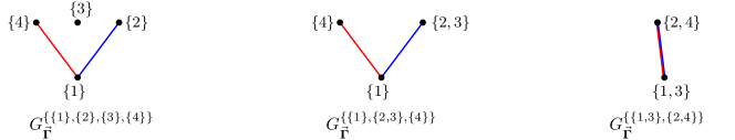
Figure 6. The first graph depicts $G^{\{\{1\},\{2\},\{3\},\{4\}\}}_{\vec{\bm{\Gamma}}}$ for the ribbon path $\vec{\bm{\Gamma}}$ from Fig. 5; observe that $\vec{\bm{\Gamma}}$ is not connected. The next two graphs $G^{\pi}_{\vec{\bm{\Gamma}}}$ correspond to other set-partitions $\pi\in\mathcal{S}\mathcal{P}([1\,..\,4])$; in both cases, $\vec{\bm{\Gamma}}$ is $\pi$-connected.

Recall that $\mathbf{L}(\ell_{1},\dots,\ell_{n})$ denotes the set of Łukasiewicz ribbon paths on $n$ sites of lengths $\ell_{1},\dots,\ell_{n}$. We denote by $\mathbf{L}^{\pi-\operatorname{conn}}(\ell_{1},\dots,\ell_{n})$ (resp. $\mathbf{L}^{\operatorname{conn}}(\ell_{1},\dots,\ell_{n})$) the subset of $\mathbf{L}(\ell_{1},\dots,\ell_{n})$ of those Łukasiewicz ribbon paths that are $\pi$-connected (resp. connected).

Proposition 3.11.

Fix arbitrary $\ell^{1}_{1},\dots,\ell^{1}_{k_{1}},\ell^{2}_{1},\dots,\ell^{2}_{k_{2}},\dots,\ell^{n}_{1},\dots,\ell^{n}_{k_{n}}\in\mathbb{Z}_{\geq 1}$. We have the following formula for a cumulant with respect to the Plancherel-type Jack measure $M^{(\alpha)}_{u;\mathbf{v}}$:

(60) $$\kappa^{(\alpha)}_{u;\mathbf{v}}\!\left(\!B_{\ell^{1}_{1}}(\Lambda_{(\alpha;u)})\cdots B_{\ell^{1}_{k_{1}}}\!\!(\Lambda_{(\alpha;u)}),\dots,B_{\ell^{n}_{1}}(\Lambda_{(\alpha;u)})\cdots B_{\ell^{n}_{k_{n}}}\!\!(\Lambda_{(\alpha;u)})\!\right)\!=\!\sum_{\vec{\bm{\Gamma}}}{F_{\frac{\alpha-1}{u},\frac{\alpha}{u^{2}},\mathbf{v}}(\vec{\bm{\Gamma}})}.$$

The sum above is over $\vec{\bm{\Gamma}}\in\mathbf{L}^{\pi-\operatorname{conn}}(\ell^{1}_{1},\dots,\ell^{1}_{k_{1}},\dots,\ell^{n}_{1},\dots,\ell^{n}_{k_{n}})$, with $|\mathbf{S}^{0}(\vec{\bm{\Gamma}})|=k_{1}+\cdots+k_{n}$, and where $\pi\in\mathcal{S}\mathcal{P}([1\,..\,k_{1}+\cdots+k_{n}])$ is the set-partition with $n$ blocks defined by $\pi:=\{[1\,..\,k_{1}],[k_{1}+1\,..\,k_{1}+k_{2}],\dots,[k_{1}+\cdots+k_{n-1}+1\,..\,k_{1}+\cdots+k_{n}]\}$, and we employed the usual notation $[a\,..\,b]:=\{a,a+1,\dots,b\}$, for any integers $a\leq b$.

Proof.

Fix the set-partition $\pi:=\{[1\,..\,k_{1}],[k_{1}+1\,..\,k_{1}+k_{2}],\dots,[k_{1}+\cdots+k_{n-1}+1\,..\,k_{1}+\cdots+k_{n}]\}$ of $[1\,..\,k_{1}+\cdots+k_{n}]$. Let $\vec{\bm{\Gamma}}\in\mathbf{L}(\ell^{1}_{1},\dots,\ell^{1}_{k_{1}},\dots,\ell^{n}_{1},\dots,\ell^{n}_{k_{n}})$ be any Łukasiewicz ribbon path. Then we can define $\sigma=\sigma(\vec{\bm{\Gamma}})\in\mathcal{S}\mathcal{P}(\pi)$ as the set-partition whose blocks are sets of vertices of the connected components of $G^{\,\pi}_{\vec{\bm{\Gamma}}}$. For each $B\in\sigma$, let $\vec{\bm{\Gamma}}_{B}$ be the concatenation of excursions $\Gamma_{b}$, $b\in\bigcup B$, with respect to the natural order. Since $\mathcal{S}\mathcal{P}(\pi)$ is isomorphic to $\mathcal{S}\mathcal{P}([1\,..\,n])$, we will denote by $\tilde{B}$ the image of a block $B\in\sigma$ by the natural map $[k_{1}+\cdots+k_{i-1}+1\,..\,k_{1}+\cdots+k_{i}]\to i$. By construction, it is evident that each $\vec{\bm{\Gamma}}_{B}$ is a well-defined, $\pi|_{B}$-connected Łukasiewicz ribbon path $\vec{\bm{\Gamma}}_{B}\in\mathbf{L}^{\pi|_{B}-\operatorname{conn}}(\ell^{b}_{1},\dots,\ell^{b}_{k_{b}}\colon b\in\tilde{B})$.

Conversely, let $\sigma\in\mathcal{S}\mathcal{P}(\pi)$ be arbitrary, and for any block $B\in\sigma$ assume that we have a $\pi|_{B}$-connected Łukasiewicz ribbon path $\vec{\bm{\Gamma}}_{B}\in\mathbf{L}^{\pi|_{B}-\operatorname{conn}}(\ell^{b}_{1},\dots,\ell^{b}_{k_{b}}\colon b\in\tilde{B})$. Then one can construct a (non-necessarily $\pi$-connected) Łukasiewicz ribbon path $\vec{\bm{\Gamma}}\in\mathbf{L}(\ell^{1}_{1},\dots,\ell^{1}_{k_{1}},\dots,\ell^{n}_{1},\dots,\ell^{n}_{k_{n}})$ as a concatenation of the excursions of lengths $\ell_{1}^{1},\dots,\ell_{k_{n}}^{n}$ that make up the $\vec{\bm{\Gamma}}_{B}$’s, and the set of pairings of $\vec{\bm{\Gamma}}$ is defined as the union of sets of pairings for $\vec{\bm{\Gamma}}_{B}$’s, for $B\in\sigma$.

Note that $F_{\,\frac{\alpha-1}{u},\,\frac{\alpha}{u^{2}},\,\mathbf{v}}(\vec{\bm{\Gamma}})=\prod_{B\in\sigma}{F_{\,\frac{\alpha-1}{u},\,\frac{\alpha}{u^{2}},\,\mathbf{v}}(\vec{\bm{\Gamma}}_{B})}$. Using Theorem 3.10, this gives:

(61) $$\mathbb{E}^{(\alpha)}_{u;\mathbf{v}}\left(B_{\ell^{1}_{1}}(\Lambda_{(\alpha;u)})\cdots B_{\ell^{1}_{k_{1}}}(\Lambda_{(\alpha;u)})\cdots B_{\ell^{n}_{1}}(\Lambda_{(\alpha;u)})\cdots B_{\ell^{n}_{k_{n}}}(\Lambda_{(\alpha;u)})\right)\\ =\sum_{\sigma\in\mathcal{S}\mathcal{P}(\pi)}\prod_{B\in\sigma}\sum_{\,\vec{\bm{\Gamma}}_{B}\in\mathbf{L}^{\pi|_{B}-\operatorname{conn}}(\ell^{b}_{1},\dots,\ell^{b}_{k_{b}}\colon b\in\tilde{B})\atop|\mathbf{S}^{0}(\vec{\bm{\Gamma}}_{B})|=\sum_{b\in\tilde{B}}k_{b}}{F_{\,\frac{\alpha-1}{u},\,\frac{\alpha}{u^{2}},\,\mathbf{v}}(\vec{\bm{\Gamma}}_{B})}.$$

Comparing this equation with (59) that defines cumulants, we conclude the proof. ∎

Corollary 3.12.

For arbitrary $\ell_{1},\dots,\ell_{n}\in\mathbb{Z}_{\geq 1}$, we have

(62) $$\kappa^{(\alpha)}_{u;\mathbf{v}}\left(S_{\ell_{1}}(\Lambda_{(\alpha;u)}),\dots,S_{\ell_{n}}(\Lambda_{(\alpha;u)})\right)=\sum_{\vec{\bm{\Gamma}}\in\mathbf{L}^{\operatorname{conn}}(\ell_{1},\dots,\ell_{n})\atop\vec{\bm{\Gamma}}=(\Gamma_{1},\dots,\Gamma_{n})}\,\prod_{j=1}^{n}\frac{1}{|\mathbf{S}^{0}(\Gamma_{j})|}\cdot F_{\,\frac{\alpha-1}{u},\,\frac{\alpha}{u^{2}},\,\mathbf{v}}(\vec{\bm{\Gamma}}).$$

Proof.

It follows immediately from Proposition 3.11 by using multilinearity of the cumulant $\kappa^{(\alpha)}_{u;\mathbf{v}}$ and (43). ∎

3.7.3. Step 3 – Concluding the proofs of Theorems 3.7 and 3.8

We start with the following:

Claim 3.13.

Any Łukasiewicz ribbon path $\vec{\bm{\Gamma}}\in\mathbf{L}(\ell_{1},\dots,\ell_{n})$ stays below height $\ell_{1}+\cdots+\ell_{n}$, i.e. $\mathbf{S}^{i}(\vec{\bm{\Gamma}})=\emptyset$, whenever $i\geq\ell_{1}+\cdots+\ell_{n}$. Moreover, $\mathbf{L}(\ell_{1},\dots,\ell_{n})$ is finite.

Proof.

The first statement easily follows from the fact that the non-paired down steps of any Łukasiewicz ribbon path have degree $1$, and we leave the details to the reader. The first statement implies that the set $\mathbf{L}(\ell_{1},\dots,\ell_{n})$ has cardinality upper bounded by $\big{(}2(\ell_{1}+\cdots+\ell_{n})+1\big{)}^{\ell_{1}+\cdots+\ell_{n}}$, and in particular is finite. ∎

End of proof of Theorem 3.7. For the LLN, i.e. Eq. 53, we first prove a general result that might be useful for studying the asymptotic behavior of random partitions in other contexts.

Let $\mathcal{M}_{<\infty}(\mathbb{R})$ be the set of positive finite measures on $\mathbb{R}$ that have finite moments of all orders. Recall that $M_{\ell}(\mu):=\int_{\mathbb{R}}{x^{\ell}d\mu(x)}$ denotes the $\ell$-th moment of the measure $\mu$.

Theorem 3.14 ([Bil95], Thm. 30.2).

Let $(\mu_{d})_{d\geq 1}\subset\mathcal{M}_{<\infty}(\mathbb{R})$ be any sequence and $\mu\in\mathcal{M}_{<\infty}(\mathbb{R})$ be a measure that is uniquely determined by its moments. Suppose that $\lim_{d\to\infty}M_{\ell}(\mu_{d})=M_{\ell}(\mu)$ for every $\ell\geq 0$, then $\mu_{d}$ converges to $\mu$ weakly.

Remark 8.

The above theorem is stated in [Bil95] for probability measures, but the proof in [Bil95] works for $\mathcal{M}_{<\infty}(\mathbb{R})$ in the same way.

Theorem 3.15.

Let $(f_{d})_{d\geq 1}$ be a sequence of random $C$-Lipschitz functions $f_{d}\colon\mathbb{R}\to\mathbb{R}_{\geq 0}$ such that $f_{d}(x)dx\in\mathcal{M}_{<\infty}(\mathbb{R})$. Suppose that

1. for every $\epsilon>0$, there exists $N>0$ such that $\lim_{d\to\infty}\mathbb{P}_{d}\left(\|f_{d}\|_{L^{\infty}(\mathbb{R}\setminus[-N,N])}>\epsilon\right)=0$,

2. there exists a measure $\mu\in\mathcal{M}_{<\infty}(\mathbb{R})$, uniquely determined by its moments, such that $f_{d}(x)dx$ converges to $\mu$ in moments, in probability, i.e. for every $\epsilon>0$ and $\ell\in\mathbb{Z}_{\geq 0}$, we have

   $$\lim_{d\to\infty}{\mathbb{P}_{d}\left(\left|\int_{\mathbb{R}}{x^{\ell}f_{d}(x)dx}-M_{\ell}(\mu)\right|>\epsilon\right)}=0.$$

Then, $(f_{d})_{d\geq 1}$ has a deterministic limit $f\colon\mathbb{R}\to\mathbb{R}_{\geq 0}$ in the supremum norm, in probability:

$$\forall\epsilon>0,\qquad\lim_{d\to\infty}\mathbb{P}_{d}\left(\|f_{d}-f\|_{\infty}>\epsilon\right)=0.$$

The function $f$ is $C$-Lipschitz, and is a probability density of the measure $\mu$.

Proof.

Step 1. Let $\epsilon>0,\,\psi\in C_{b}(\mathbb{R})$ be arbitrary. In this step, we show that (b) implies

(63) $$\lim_{d\to\infty}{\mathbb{P}_{d}\left(\left|\int_{\mathbb{R}}{\psi(x)f_{d}(x)dx}-\int_{\mathbb{R}}{\psi(x)d\mu(x)}\right|\leq\epsilon\right)}=1.$$

Consider the following metric $\pi$ on $\mathcal{M}_{<\infty}(\mathbb{R})$:

$$\pi(\nu_{1},\nu_{2}):=\sum_{i=0}^{\infty}\frac{\min\left(1,\,|M_{i}(\nu_{1})-M_{i}(\nu_{2})|\right)}{2^{i}}.$$

From the definition of $\pi$, it follows that for any $\epsilon>0$, there exist $\epsilon^{\prime}>0,\,k\in\mathbb{Z}_{\geq 1}$ such that:

$$\text{ if $\nu\in\mathcal{M}_{<\infty}(\mathbb{R})$ satisfies }\ |M_{1}(\nu)-M_{1}(\mu)|,\dots,|M_{k}(\nu)-M_{k}(\mu)|\leq\epsilon^{\prime}\Longrightarrow\pi(\nu,\mu)\leq\epsilon.$$

As a result, $\pi$ metrizes convergence in moments, so that the assumption (b) is equivalent to the following condition: for every $\epsilon>0$, we have

(64) $$\lim_{d\to\infty}{\mathbb{P}_{d}\left(\pi(f_{d}(x)dx,\mu)\leq\epsilon\right)}=1.$$

A classical theorem of Lev́y says that the weak convergence in $\mathcal{M}_{<\infty}(\mathbb{R})$ is metrizable (see [Var58] for a more general result); let $\tilde{\pi}$ denote the corresponding metric. In other terms, for any sequence of measures $(\nu_{n})_{n\geq 1}\subset\mathcal{M}_{<\infty}(\mathbb{R})$ one has $\nu_{n}\to\mu$ weakly, if and only if $\tilde{\pi}(\nu_{n},\mu)\to 0$, as $n\to\infty$. Consequently, (63) would be implied if for every $\epsilon^{\prime}>0$, we have

(65) $$\lim_{d\to\infty}{\mathbb{P}_{d}\left(\tilde{\pi}(f_{d}(x)dx,\mu)\leq\epsilon^{\prime}\right)}=1.$$

Note that Theorem 3.14 implies that for any $\epsilon^{\prime}>0$, there exists $\epsilon>0$ such that $\pi(\nu,\mu)\leq\epsilon\Longrightarrow\tilde{\pi}(\nu,\mu)\leq\epsilon^{\prime}$. Therefore $\mathbb{P}_{d}\left(\pi(f_{d}(x)dx,\mu)\leq\epsilon\right)\leq\mathbb{P}_{d}\left(\tilde{\pi}(f_{d}(x)dx,\mu)\leq\epsilon^{\prime}\right)$, and (64) implies the desired limit (65).

Step 2. Fix $x_{0}\in\mathbb{R}$ and let $\psi_{\epsilon}^{x_{0}}\in C_{c}(\mathbb{R})$ be a nonnegative function supported on $[x_{0}-\epsilon,x_{0}+\epsilon]$ with $\int_{\mathbb{R}}\psi_{\epsilon}^{x_{0}}(x)dx=1$ For any $C$-Lipschitz function $g$, one has

$$\left|g(x_{0})-\int_{\mathbb{R}}{\psi_{\epsilon}^{x_{0}}(x)g(x)dx}\right|\leq\!\int_{\mathbb{R}}{\psi_{\epsilon}^{x_{0}}(x)|g(x_{0})-g(x)|dx}\leq C\epsilon,$$

therefore

$$\left|g(x_{0})-\!\int_{\mathbb{R}}\psi_{\epsilon}^{x_{0}}(x)d\mu(x)\right|\leq C\epsilon+\left|\int_{\mathbb{R}}{\psi_{\epsilon}^{x_{0}}(x)g(x)dx}-\int_{\mathbb{R}}{\psi_{\epsilon}^{x_{0}}(x)d\mu(x)}\right|.$$

When we take $g=f_{d}$ we obtain

$$\mathbb{P}_{d}\!\left(\left|f_{d}(x_{0})\!-\!\int_{\mathbb{R}}\psi_{\epsilon}^{x_{0}}(x)d\mu(x)\right|\!\leq\!(C+1)\epsilon\!\right)\!\geq\!\mathbb{P}_{d}\!\left(\left|\int_{\mathbb{R}}\psi_{\epsilon}^{x_{0}}(x)f_{d}(x)dx\!-\!\int_{\mathbb{R}}\psi_{\epsilon}^{x_{0}}(x)d\mu(x)\right|\!\leq\!\epsilon\!\right)\!.$$

Step 1 shows that this RHS above converges to $1$, as $d\to\infty$. Consequently, for any $\epsilon>0$, we have: $\lim_{d\to\infty}\mathbb{P}_{d}\left(|f_{d}(x_{0})-\int_{\mathbb{R}}\psi_{\epsilon}^{x_{0}}(x)d\mu(x)|\leq(C+1)\epsilon\right)=1$. Passing to the limit $\epsilon\to 0$, we get that

$$\lim_{d\to\infty}f_{d}(x_{0})=f(x_{0}):=\lim_{\epsilon\to 0}\int_{\mathbb{R}}\psi_{\epsilon}^{x_{0}}(x)d\mu(x),$$

where the first equality holds in probability. Since $x_{0}$ was arbitrary, we have a pointwise convergence $f_{d}\to f$, in probability. This pointwise convergence can be extended to the uniform convergence on any closed interval, in probability, by a standard argument of covering a closed interval by finitely many small intervals, and the fact that that the supremum norm of $|f_{d}-f|$ on a small interval is small by the Lipschitz condition. Therefore for every $N,\epsilon>0$

$$\lim_{d\to\infty}\mathbb{P}_{d}\left(\|f_{d}-f\|_{L^{\infty}[-N,N]}>\epsilon\right)=0.$$

Finally, fix any $\epsilon>0$ and take $N>0$ as in condition (a) from the hypothesis; then

$$\mathbb{P}_{d}\left(\|f_{d}-f\|_{\infty}>\epsilon\right)\leq\mathbb{P}_{d}\left(\|f_{d}-f\|_{L^{\infty}[-N,N]}>\epsilon\right)+\mathbb{P}_{d}\left(\|f_{d}-f\|_{L^{\infty}(\mathbb{R}\setminus[-N,N])}>\epsilon\right)\to 0$$

as $d\to\infty$. Since the functions $f_{d}$ are $\geq 0$ and $C$-Lipschitz, $f$ has the same properties.

Step 3. It remains to show that $f$ is the density of $\mu$. As $\mu$ is uniquely determined by its moments, it suffices to verify $\int_{\mathbb{R}}{x^{\ell}f(x)dx}=M_{\ell}(\mu)$, for all $\ell\in\mathbb{Z}_{\geq 0}$. Fix $\ell\geq 0$ and $R>0$,

$$\left|\int_{|x|\geq R}{\!x^{\ell}f_{d}(x)dx}\right|\leq\int_{|x|\geq R}{\!|x|^{\ell}f_{d}(x)dx}\leq\int_{|x|\geq R}{\!\frac{|x|^{2\ell+2}}{R^{\ell+2}}f_{d}(x)dx}=\!\frac{1}{R^{\ell+2}}\!\int_{|x|\geq R}{\!x^{2\ell+2}f_{d}(x)dx}$$

$$\leq\frac{1}{R^{\ell+2}}\int_{\mathbb{R}}{x^{2\ell+2}f_{d}(x)dx}\leq\frac{1}{R^{\ell+2}}\left|\int_{\mathbb{R}}{x^{2\ell+2}f_{d}(x)dx}-M_{2\ell+2}(\mu)\right|+\frac{M_{2\ell+2}(\mu)}{R^{\ell+2}}.$$

This inequality and condition (b) show that for any $\epsilon>0$, there exists $R_{0}>0$ such that

(66) $$\lim_{d\to\infty}{\mathbb{P}_{d}\left(\left|\int_{|x|\geq R}{x^{\ell}f_{d}(x)dx}\right|<\epsilon\right)}=1,\quad\forall\,R>R_{0}.$$

Note that $\left|M_{\ell}(\mu)-\int_{|x|\leq R}{x^{\ell}f(x)dx}\right|$ is bounded from above by

$$\bigg{|}M_{\ell}(\mu)-M_{\ell}(f_{d}(x)dx)\bigg{|}+\left|\int_{|x|\geq R}{x^{\ell}f_{d}(x)dx}\right|+\left|\int_{-R}^{R}x^{\ell}(f_{d}(x)-f(x))dx\right|.$$

For any $\epsilon>0$, there exists $R_{0}>0$ such that for every $R>R_{0}$ the probability $\mathbb{P}_{d}$ that each of these terms is smaller than $\epsilon$ tends to $1$, as $d\to\infty$. Indeed, for the first term this is condition (b), for the second this is (66), and for the third one this is convergence of $f_{d}\to f$ uniformly on $[-R,R]$ in probability, proved in Step 2. Taking the limit as $R\to\infty$, it follows that the integral $\int_{\mathbb{R}}{x^{\ell}f(x)dx}$ converges and equals $M_{\ell}(\mu)$, as desired. ∎

We are going to prove Theorem 3.7 by applying Theorem 3.15 to the collection of functions

$$f_{(\alpha;u\cdot{\sqrt{v_{1}}})}(x):=\frac{\omega_{\Lambda_{(\alpha;u\cdot\sqrt{v_{1}})}}(x)-|x|}{2},\quad x\in\mathbb{R},$$

that are parametrized by an integer $d\geq 1$ (recall that $\alpha=\alpha(d),\,u=u(d)$). In our setting, $\lambda$ is an $M^{(\alpha)}_{u;\mathbf{v}}$-distributed random partition, and $\Lambda_{(\alpha;u\cdot\sqrt{v_{1}})}:=T_{\frac{\alpha}{u\cdot\sqrt{v_{1}}},\frac{1}{u\cdot\sqrt{v_{1}}}}\lambda$, therefore $(f_{(\alpha;u\cdot{\sqrt{v_{1}}})})_{d\geq 1}\colon\mathbb{R}\to\mathbb{R}_{\geq 0}$ is a collection of random $1$–Lipschitz compactly supported functions. Let us verify the two conditions required by Theorem 3.7.

Step 1: For every $\epsilon>0$, there exists $N>0$ such that

$$\lim_{d\to\infty}{M^{(\alpha)}_{u;\mathbf{v}}\left(\|f_{(\alpha;u\cdot{\sqrt{v_{1}}})}\|_{L^{\infty}(\mathbb{R}\setminus[-N,N])}>\epsilon\right)}=0.$$

Let $U=U(d):=\frac{u^{2}\cdot v_{1}}{\alpha}$. Note that if the point $(x_{0},y_{0})$ in the first quadrant belongs to the rescaled diagram $\Lambda_{(\alpha;u\cdot\sqrt{v_{1}})}$, then the whole rectangle $(0,0)$–$(x_{0},0)$–$(x_{0},y_{0})$–$(0,y_{0})$ is contained in $\Lambda_{(\alpha;u\cdot\sqrt{v_{1}})}$, therefore $x_{0}\cdot y_{0}\leq|\Lambda_{(\alpha;u\cdot\sqrt{v_{1}})}|=\frac{|\lambda|}{U}$. Applying this inequality to $x_{0}=(\omega_{\Lambda_{(\alpha;u\cdot\sqrt{v_{1}})}}(x)+|x|)/2\,$ and $y_{0}=(\omega_{\Lambda_{(\alpha;u\cdot\sqrt{v_{1}})}}(x)-|x|)/2$, we obtain

$$|x|\leq\omega_{\Lambda_{(\alpha;u\cdot\sqrt{v_{1}})}}(x)\leq\sqrt{x^{2}+4\cdot\frac{|\lambda|}{U}},$$

and consequently

(67) $$0\leq f_{(\alpha;u\cdot{\sqrt{v_{1}}})}(x)\leq\frac{\sqrt{x^{2}+4\cdot\frac{|\lambda|}{U}}-|x|}{2}\leq\frac{\sqrt{x^{2}+8e}-|x|}{2}=\frac{4e}{\sqrt{x^{2}+8e}+|x|},$$

whenever $|\lambda|\leq 2e\cdot U$. Note that for every $\epsilon>0$, there exists $N>0$ such that the RHS of (67) is smaller or equal to $\epsilon$, for all $|x|\geq N$. Therefore it is enough to prove that

(68) $$\lim_{d\to\infty}M^{(\alpha)}_{u;\mathbf{v}}\left(|\lambda|>2e\cdot U\right)=0.$$

By looking at the coefficient of $t^{i}$ in the Cauchy identity (31), we deduce that the measure $M^{(\alpha)}_{u;\mathbf{v}}$ gives $\mathbb{Y}_{i}$ a mass of $e^{-U}\cdot\frac{U^{i}}{i!}$, therefore for any $k\in\mathbb{Z}_{\geq 1}$, one has

$$M^{(\alpha)}_{u;\mathbf{v}}\left(|\lambda|>k\right)\leq\exp(-U)\sum_{i=k}^{\infty}\frac{U^{i}}{i!}\leq\frac{U^{k}}{k!}=O\left(\left(\frac{e\cdot U}{k}\right)^{\!k}\cdot k^{-\frac{1}{2}}\right)\!,\text{ as }k\to\infty,$$

where the last equality follows from the Stirling’s formula. Observe that our assumptions (51) imply that $U\to\infty$ as $d\to\infty$, therefore if we choose $k:=\lfloor 2e\cdot U\rfloor$, then also $k\to\infty$ as $d\to\infty$. We conclude that (68) holds true, and this finishes the proof of this step.

Step 2: There exists a probability measure $P_{\infty}\in\mathcal{M}_{<\infty}(\mathbb{R})$ such that $f_{(\alpha;u\cdot{\sqrt{v_{1}}})}(x)dx$ converges to $P_{\infty}$ in moments, in probability.

Consider the function $\mathbb{E}^{(\alpha)}_{u;\mathbf{v}}[f_{(\alpha;u\cdot{\sqrt{v_{1}}})}(x)]$, which for simplicity we denote $\mathbb{E}[f(x)]$. Eq. 46 shows that, for any $\ell\in\mathbb{Z}_{\geq 0}$, we have

(69) $$\int_{\mathbb{R}}{x^{\ell}\,\mathbb{E}[f(x)]dx}=\mathbb{E}\left[\!\int_{\mathbb{R}}{x^{\ell}f(x)dx}\right]\!=\!\frac{\mathbb{E}\left[S_{\ell+2}(\Lambda_{(\alpha;u\cdot\sqrt{v_{1}})})\right]}{\ell+1}.$$

When $\ell=0$, this shows $\int_{-\infty}^{\infty}{\mathbb{E}[f(x)]dx}=\mathbb{E}[S_{2}(\Lambda_{(\alpha;u\cdot\sqrt{v_{1}})})]=v_{1}^{-1}\cdot\mathbb{E}[S_{2}(\Lambda_{(\alpha;u)})]$ and this equals $1$, by Eq. 62. Therefore $\mathbb{E}[f(x)]$ is the density of a probability measure, to be denoted by $P_{d}$.

Since $\mathbf{L}^{\operatorname{conn}}(\ell)=\mathbf{L}(\ell)$ is finite and $S_{\ell}(\Lambda_{(\alpha;u\cdot\sqrt{v_{1}})})=v_{1}^{-\ell/2}\cdot S_{\ell}(\Lambda_{(\alpha;u)})$, then Eq. 62 shows that the following limits exist:

(70) $$\lim_{d\to\infty}\mathbb{E}^{(\alpha)}_{u;\mathbf{v}}\left[S_{\ell}(\Lambda_{(\alpha;u\cdot\sqrt{v_{1}})})\right]=v_{1}^{-\frac{\ell}{2}}\lim_{d\to\infty}\kappa^{(\alpha)}_{u;\mathbf{v}}\left(S_{\ell}(\Lambda_{(\alpha;u)})\right)\\ =v_{1}^{-\frac{\ell}{2}}\sum_{\Gamma\in\mathbf{L}_{0}(\ell)}\frac{1}{|\mathbf{S}^{0}(\Gamma)|}\prod_{i\geq 1}(i\cdot g)^{|\mathbf{S}^{i}_{\tiny\rightarrow}(\Gamma)|}\,v_{i}^{\,|\mathbf{S}_{i}(\Gamma)|},$$

for all $\ell\in\mathbb{Z}_{\geq 1}$. Note that since $\alpha/u^{2}\to 0$, then the only paths that survive from (62) are the ones with $|\mathbf{P}(\vec{\bm{\Gamma}})|=0$; this explains why after taking the limit as $d\to\infty$, the sum above is over $\Gamma\in\mathbf{L}_{0}(\ell)$ (with no pairings) and not over $\Gamma\in\mathbf{L}(\ell)$. Similarly, note that any Łukasiewicz ribbon path $\vec{\bm{\Gamma}}\in\mathbf{L}^{\operatorname{conn}}(\ell_{1},\ell_{2})$ must have at least $1$ pairing for the connectivity condition to hold, i.e. $|\mathbf{P}(\vec{\bm{\Gamma}})|=\sum_{i\geq 1}{|\mathbf{P}_{i}(\vec{\bm{\Gamma}})|}\geq 1$, therefore Eq. 62 also implies

(71) $$\lim_{d\to\infty}\text{Var}^{(\alpha)}_{u;\mathbf{v}}\left[S_{\ell}(\Lambda_{(\alpha;u\cdot\sqrt{v_{1}})})\right]=v_{1}^{-\ell}\lim_{d\to\infty}{\kappa^{(\alpha)}_{u;\mathbf{v}}\left(S_{\ell}(\Lambda_{(\alpha;u)}),S_{\ell}(\Lambda_{(\alpha;u)})\right)}=0.$$

From (70), (71), and Chebyshev’s inequality, we have that for any $\epsilon>0$ and any $\ell\in\mathbb{Z}_{\geq 1}$,

(72) $$\lim_{d\to\infty}{M^{(\alpha)}_{u;\mathbf{v}}\left(|S_{\ell}(\Lambda_{(\alpha;u\cdot\sqrt{v_{1}})})-s_{\ell}|\geq\epsilon\right)}=0,$$

where

(73) $$s_{\ell}:=v_{1}^{-\frac{\ell}{2}}\sum_{\Gamma\in\mathbf{L}_{0}(\ell)}\frac{1}{|\mathbf{S}^{0}(\Gamma)|}\prod_{i\geq 1}(i\cdot g)^{|\mathbf{S}^{i}_{\tiny\rightarrow}(\Gamma)|}\,v_{i}^{\,|\mathbf{S}_{i}(\Gamma)|}.$$

Next, observe that (69), (70) and (71) imply that the moments and variances of the measures $P_{d}$ are uniformly bounded. Thus $(P_{d})_{d\geq 1}$ is a tight sequence of probability measures, and thus it contains a subsequence $(P_{d_{k}})_{k\geq 1}$ that converges weakly to some probability measure $P_{\infty}$. The limit (70) shows further that the $\ell$-th moment of $P_{\infty}$ is $\frac{s_{\ell+2}}{\ell+1}$, for all $\ell\geq 0$. Finally (69) and (72) imply that for any $\epsilon>0$ and any $\ell\in\mathbb{Z}_{\geq 1}$, we have that

$$\lim_{d\to\infty}{M^{(\alpha)}_{u;\mathbf{v}}\left(\left|\int_{\mathbb{R}}{x^{\ell}f_{(\alpha;u\cdot\sqrt{v_{1}})}(x)dx}-\int_{\mathbb{R}}{x^{\ell}P_{\infty}(dx)}\right|\geq\epsilon\right)}=0.$$

In Section 6, we show that $P_{\infty}$ is uniquely determined by its moments (see Corollary 6.3), which finishes the proof.

Step 3: Conclusion of the argument.

Steps 1 and 2 prove that the two conditions in Theorem 3.15 are satisfied for the sequence $(f_{(\alpha;u\cdot{\sqrt{v_{1}}})})_{d\geq 1}$ and $\mu=P_{\infty}$. Consequently, there exists a deterministic function $f_{\Lambda_{g;\mathbf{v}}}:\mathbb{R}\to\mathbb{R}_{\geq 0}$, which is a probability density function of $P_{\infty}$, such that for every $\epsilon>0$:

$$\lim_{d\to\infty}M^{(\alpha)}_{u;\mathbf{v}}\left(\|f_{(\alpha;u\cdot{\sqrt{v_{1}}})}-f_{\Lambda_{g;\mathbf{v}}}\|_{\infty}>\epsilon\right)=0.$$

Consequently, setting $\omega_{\Lambda_{g;\mathbf{v}}}(x):=2f_{\Lambda_{g;\mathbf{v}}}(x)+|x|$, we conclude the convergence of $\omega_{\Lambda_{(\alpha;u\cdot{\sqrt{v_{1}}})}}$ to $\omega_{\Lambda_{g;\mathbf{v}}}$ in the supremum norm, in probability.

Finally, the fact that formula (54) gives the moments of the associated transition measure $\mu_{g;\mathbf{v}}$ follows from Markov–Krein correspondence (Theorem 3.3) and Proposition 3.2.

End of proof of Theorem 3.8. For the CLT, let us first prove the following limits:

(74) $$\lim_{d\to\infty}\ \kappa^{(\alpha)}_{u;\mathbf{v}}\left(\langle\Delta^{(\alpha)}_{u;\mathbf{v}},x^{k-2}\rangle,\langle\Delta^{(\alpha)}_{u;\mathbf{v}},x^{l-2}\rangle\right)=\frac{v_{1}^{-\frac{k+l}{2}}}{(k-1)(l-1)}\times$$

$$\times \sum_{\vec{\bm{\Gamma}}=(\Gamma_{1},\Gamma_{2})\in\mathbf{L}^{\operatorname{conn}}(k,l)\atop|\mathbf{P}(\vec{\bm{\Gamma}})|=1}\frac{1}{|\mathbf{S}^{0}(\Gamma_{1})||\mathbf{S}^{0}(\Gamma_{2})|}\prod_{i\geq 1}(i\cdot g)^{|\mathbf{S}_{\tiny\rightarrow}^{i}(\vec{\bm{\Gamma}})|}\,i^{\,|\mathbf{P}_{i}(\vec{\bm{\Gamma}})|}\,v_{i}^{\,|\mathbf{S}_{i}(\vec{\bm{\Gamma}})|},\quad\forall\,k,l\geq 2,$$

(75) $$\lim_{d\to\infty}\ \kappa^{(\alpha)}_{u;\mathbf{v}}\left(\langle\Delta^{(\alpha)}_{u;\mathbf{v}},x^{\ell_{1}-2}\rangle,\dots,\langle\Delta^{(\alpha)}_{u;\mathbf{v}},x^{\ell_{n}-2}\rangle\right)=0,\quad\forall\,n>2,\ \forall\,\ell_{1},\cdots,\ell_{n}\geq 2.$$

In order to compute

$$\lim_{d\to\infty}\kappa^{(\alpha)}_{u;\mathbf{v}}\left(\langle\Delta^{(\alpha)}_{u;\mathbf{v}},x^{\ell_{1}-2}\rangle,\dots,\langle\Delta^{(\alpha)}_{u;\mathbf{v}},x^{\ell_{n}-2}\rangle\right)$$

for $n\geq 2$, first use the fact that the cumulant $\kappa^{(\alpha)}_{u;\mathbf{v}}$ of order $n\geq 2$ is invariant by any translation of any argument by a scalar, so that using also (46) we have the following equalities

(76) $$\kappa^{(\alpha)}_{u;\mathbf{v}}\left(\langle\Delta^{(\alpha)}_{u;\mathbf{v}},x^{\ell_{1}-2}\rangle,\dots,\langle\Delta^{(\alpha)}_{u;\mathbf{v}},x^{\ell_{n}-2}\rangle\right)\\ =\left(\frac{u}{\sqrt{\alpha}}\right)^{\!n}\cdot\,\kappa^{(\alpha)}_{u;\mathbf{v}}\left(\langle f_{(\alpha;u\cdot\sqrt{v_{1}})},x^{\ell_{1}-2}\rangle,\dots,\langle f_{(\alpha;u\cdot\sqrt{v_{1}})},x^{\ell_{n}-2}\rangle\right)\\ =\left(\frac{u}{\sqrt{\alpha}}\right)^{\!n}\cdot\prod_{i=1}^{n}\frac{1}{(\ell_{i}-1)}\cdot\kappa^{(\alpha)}_{u;\mathbf{v}}\left(S_{\ell_{1}}(\Lambda_{(\alpha;u\cdot\sqrt{v_{1}})}),\dots,S_{\ell_{n}}(\Lambda_{(\alpha;u\cdot\sqrt{v_{1}})})\right).$$

Next, use the scaling property (44) that shows $S_{\ell}(\Lambda_{(\alpha;u\cdot\sqrt{v_{1}})})=v_{1}^{-\frac{\ell}{2}}\cdot S_{\ell}(\Lambda_{(\alpha;\sqrt{v_{1}})})$, and then (62) from Corollary 3.12. Note that the sum in the last equation is over connected Łukasiewicz ribbon paths $\vec{\bm{\Gamma}}\in\mathbf{L}^{\operatorname{conn}}(\ell_{1},\dots,\ell_{n})$ on $n$ sites, and each such $\vec{\bm{\Gamma}}$ must have at least $(n-1)$ pairings for it to be connected, i.e. $|\mathbf{P}(\vec{\bm{\Gamma}})|=\sum_{i\geq 1}{|\mathbf{P}_{i}(\vec{\bm{\Gamma}})|}\geq n-1$. As a result:

(77) $$\kappa^{(\alpha)}_{u;\mathbf{v}}\left(S_{\ell_{1}}(\Lambda_{(\alpha;u\cdot\sqrt{v_{1}})}),\dots,S_{\ell_{n}}(\Lambda_{(\alpha;u\cdot\sqrt{v_{1}})})\right)=\bigg{(}\frac{\alpha}{u^{2}}\bigg{)}^{\!n-1}\cdot v_{1}^{-\frac{\ell_{1}+\cdots+\ell_{n}}{2}}\times\\ \times\Bigg{(}\sum_{\vec{\bm{\Gamma}}\in\mathbf{L}^{\operatorname{conn}}(\ell_{1},\dots,\ell_{n}),\atop|\mathbf{P}(\vec{\bm{\Gamma}})|=n-1}\prod_{j=1}^{n}\frac{1}{|\mathbf{S}^{0}(\Gamma_{j})|}\prod_{i\geq 1}\bigg{(}i\cdot\frac{\alpha-1}{u}\bigg{)}^{\!|\mathbf{S}^{i}_{\tiny\rightarrow}(\vec{\bm{\Gamma}})|}i^{\,|\mathbf{P}_{i}(\vec{\bm{\Gamma}})|}\,v_{i}^{\,|\mathbf{S}_{i}(\vec{\bm{\Gamma}})|}+\frac{\alpha}{u^{2}}\cdot X_{n}\Bigg{)},$$

where $X_{n}$ is some polynomial in $\mathbb{Q}[\frac{\alpha}{u^{2}},\frac{\alpha-1}{u},v_{1},v_{2},\dots]$. By combining (76) and (77), we have an expression of the form

$$\kappa^{(\alpha)}_{u;\mathbf{v}}\left(\langle\Delta^{(\alpha)}_{u;\mathbf{v}},x^{\ell_{1}-2}\rangle,\dots,\langle\Delta^{(\alpha)}_{u;\mathbf{v}},x^{\ell_{n}-2}\rangle\right)=\bigg{(}\frac{\sqrt{\alpha}}{u}\bigg{)}^{\!n-2}\cdot\frac{v_{1}^{-\frac{\ell_{1}+\cdots+\ell_{n}}{2}}}{\prod_{i=1}^{n}{(\ell_{i}-1)}}\cdot\left(Y_{n}+\frac{\alpha}{u^{2}}\cdot X_{n}\right),$$

where $Y_{n}$ is the sum in the RHS of Eq. 77. Notice that $X_{n}$ and $Y_{n}$ have finite limits as $d\to\infty$: in fact, just replace $\frac{\alpha-1}{u}\mapsto g,\,\frac{\alpha}{u^{2}}\mapsto 0$ in their expressions. By taking the $d\to\infty$ limit of this equation, we obtain (74) and (75).

To conclude the theorem, we show that $\,\lim_{d\to\infty}{\kappa^{(\alpha)}_{u;\mathbf{v}}(\langle\Delta^{(\alpha)}_{u;\mathbf{v}},x^{\ell-2}\rangle)}$ is equal to the RHS of Eq. 55. Let us use the notations inside the proof of Theorem 3.7. By definition, $\Delta^{(\alpha)}_{u;\mathbf{v}}=\frac{u}{2\sqrt{\alpha}}(\omega_{\Lambda_{(\alpha;\,u\cdot\sqrt{v_{1}})}}-\omega_{\Lambda_{g;\mathbf{v}}})=\frac{u}{\sqrt{\alpha}}(f_{(\alpha;\,u\cdot\sqrt{v_{1}})}-f_{g;\mathbf{v}})$. Together with (46) and (44), we obtain

$$\kappa^{(\alpha)}_{u;\mathbf{v}}\left(\langle\Delta^{(\alpha)}_{u;\mathbf{v}},x^{\ell-2}\rangle\right) =\frac{u}{\sqrt{\alpha}}\cdot\left\{\kappa^{(\alpha)}_{u;\mathbf{v}}\left(\langle f_{(\alpha;u\cdot\sqrt{v_{1}})},x^{\ell-2}\rangle\right)-\langle f_{g;\mathbf{v}},x^{\ell-2}\rangle\right\}$$

(78) $$=\frac{u}{\sqrt{\alpha}}\cdot\left\{\frac{v_{1}^{-\ell/2}}{\ell-1}\cdot\mathbb{E}^{(\alpha)}_{u;\mathbf{v}}\left[S_{\ell}(\Lambda_{(\alpha;u)})\right]-\frac{s_{\ell}}{\ell-1}\right\}.$$

By (62) and (73), the expression inside brackets in (78) can be written as a sum of weighted ribbon paths in $\mathbf{L}(\ell)$. Let $U$ be the sum over those $\vec{\bm{\Gamma}}\in\mathbf{L}(\ell)$ with $|\mathbf{P}(\vec{\bm{\Gamma}})|\geq 1$, and $V$ the sum over those with $|\mathbf{P}(\vec{\bm{\Gamma}})|=0$. Note that $U=\frac{\alpha}{u^{2}}\cdot U^{\prime}$, for some $U^{\prime}\in\mathbb{Q}[\frac{\alpha-1}{u},\frac{\alpha}{u^{2}},v_{1}^{-1/2},\{v_{i}\}_{i\geq 1}]$. On the other hand, $V=\widetilde{V}(\frac{\alpha-1}{u})-\widetilde{V}(g)$, where $\widetilde{V}(g)$ is the polynomial expression for $\frac{s_{\ell}}{\ell-1}$, see (73), and therefore $V=\left(\frac{\alpha-1}{u}-g\right)\cdot V^{\prime}$, for some $V^{\prime}\in\mathbb{Q}[\frac{\alpha-1}{u},g,v_{1}^{-1/2},\{v_{i}\}_{i\geq 1}]$.

Then the expression in brackets equals $\frac{\alpha}{u^{2}}\cdot U^{\prime}+\left(\frac{\alpha-1}{u}-g\right)\cdot V^{\prime}$, and it follows that

(79) $$\kappa^{(\alpha)}_{u;\mathbf{v}}\left(\langle\Delta^{(\alpha)}_{u;\mathbf{v}},x^{\ell-2}\rangle\right)=\frac{\sqrt{\alpha}}{u}\cdot U^{\prime}+\frac{u}{\sqrt{\alpha}}\left(\frac{\alpha-1}{u}-g\right)\cdot V^{\prime}.$$

Both $U^{\prime}$ and $V^{\prime}$ have finite limits as $d\to\infty$ and moreover, by the refined version of 3.6, $\frac{\sqrt{\alpha}}{u}=\frac{1}{\sqrt{d}}(1+o(1)),\,\frac{u}{\sqrt{\alpha}}=\sqrt{d}(1+o(1)),\,\frac{\alpha-1}{u}-g=\frac{g^{\prime}}{\sqrt{d}}(1+o(1))$; they imply that $\,\lim_{d\to\infty}{\kappa^{(\alpha)}_{u;\mathbf{v}}(\langle\Delta^{(\alpha)}_{u;\mathbf{v}},x^{\ell-2}\rangle)}=g^{\prime}\cdot\lim_{d\to\infty}{V^{\prime}}$. But $\lim_{d\to\infty}{V^{\prime}}=\lim_{\frac{\alpha-1}{u}\to g}{(\widetilde{V}(\frac{\alpha-1}{u})-\widetilde{V}(g))(\frac{\alpha-1}{u}-g)^{-1}}=\frac{\partial}{\partial g}\widetilde{V}(g)$. Hence, we have finally obtained the RHS of Eq. 55, and have thus concluded the proof of the CLT.

4. Parameters for Plancherel-type Jack measures

In this section, we investigate possible choices of parameters $u>0,\,\mathbf{v}\in\mathbb{R}^{\infty}$, for which the Plancherel-type Jack measures $M^{(\alpha)}_{u;\mathbf{v}}$ from Definition 3.5 are well-defined probability measures, both for fixed $\alpha>0$, and for all $\alpha>0$. Moreover, we find large families of parameters for which 3.6 is satisfied.

4.1. Jack-positive specializations

A specialization of the $\mathbb{R}$-algebra of symmetric functions $\operatorname{Sym}$ is by definition a unital algebra homomorphism $\rho:\operatorname{Sym}\to\mathbb{R}$. Since $\operatorname{Sym}=\mathbb{R}[p_{1},p_{2},\cdots]$, then $\rho$ is uniquely determined by the values $\rho(p_{1}),\rho(p_{2}),\cdots$. If we set $v_{k}:=\rho(p_{k})$, for all $k\in\mathbb{Z}_{\geq 1}$, and $\mathbf{v}:=(v_{1},v_{2},\cdots)$, we say that $\mathbf{v}$ determines the specialization $\rho$. For any $f\in\operatorname{Sym}$, we denote its image under $\rho$ by either $\rho(f)$ or $f(\mathbf{v})$.

Definition 4.1.

The specialization $\rho:\operatorname{Sym}\to\mathbb{R}$ is an $\boldsymbol{\alpha}$-Jack-positive specialization if

$$\rho\left(J_{\lambda}^{(\alpha)}\right)\geq 0\quad\forall\,\lambda\in\mathbb{Y}.$$

Observe that the previous definition depends on the value of $\alpha>0$.

Theorem 4.2 (Kerov-Okounkov-Olshanski [KOO98]).

Assume that $\alpha>0$ is fixed. The set of $\alpha$-Jack-positive specializations $\rho:\operatorname{Sym}\to\mathbb{R}$ is in bijection with the Thoma cone

$$\Omega=\{(a,b,c)\in\mathbb{R}^{\infty}\times\mathbb{R}^{\infty}\times\mathbb{R}\mid a=(a_{1},a_{2},\cdots),\quad b=(b_{1},b_{2},\cdots),\\ a_{1}\geq a_{2}\geq\cdots\geq 0,\quad b_{1}\geq b_{2}\geq\cdots\geq 0,\quad\sum_{i=1}^{\infty}{(a_{i}+b_{i})}\leq c\}.$$

For any $\omega=(a,b,c)\in\Omega$, the corresponding $\alpha$-Jack-positive specialization $\rho_{\omega}\!:\operatorname{Sym}\to\mathbb{R}$ is defined by

$$\rho_{\omega}(p_{1})=c,\qquad\rho_{\omega}(p_{k})=\sum_{i=1}^{\infty}{a_{i}^{k}}+(-\alpha)^{1-k}\sum_{i=1}^{\infty}{b_{i}^{k}},\quad k=2,3,\cdots.$$

Example 2.

Given $u>0$, the Plancherel $u$-specialization $\tau_{u}:\operatorname{Sym}\to\mathbb{R}$ is defined by

$$\tau_{u}(p_{1})=u,\qquad\tau_{u}(p_{2})=\tau_{u}(p_{3})=\cdots=0.$$

This is the $\alpha$-Jack-positive specialization corresponding to $c=u$, and $a_{i}=b_{i}=0,\ \forall\,i\geq 1$, in Theorem 4.2.

Example 3.

For any infinite tuple $\mathbf{v}=(v_{1},v_{2},\cdots)\in\mathbb{R}^{\infty}$ and $u\in\mathbb{R}$, recall that $u\cdot\mathbf{v}:=(uv_{1},uv_{2},\cdots)$. We claim that if $\mathbf{v}=(v_{1},v_{2},\cdots)\in\mathbb{R}^{\infty}$ determines an $\alpha$-Jack-positive specialization and if $m\in\mathbb{Z}_{>0}$, then $m\cdot\mathbf{v}$ determines another $\alpha$-Jack-positive specialization. In fact, let $(a,b,c)\in\Omega$,  $a=(a_{1},a_{2},\cdots)$,  $b=(b_{1},b_{2},\cdots)$, be the triple corresponding to $\mathbf{v}$, as given by Theorem 4.2. Then $m\cdot\mathbf{v}$ corresponds to the triple $(a^{\otimes m},b^{\otimes m},m\cdot c)\in\Omega$, where

$$a^{\otimes m}:=(\underbrace{a_{1},\cdots,a_{1}}_{m\text{ times}},\underbrace{a_{2},\cdots,a_{2}}_{m\text{ times}},a_{3},\cdots),\quad b^{\otimes m}:=(\underbrace{b_{1},\cdots,b_{1}}_{m\text{ times}},\underbrace{b_{2},\cdots,b_{2}}_{m\text{ times}},b_{3},\cdots).$$

Example 4.

For any infinite tuple $\mathbf{v}=(v_{1},v_{2},\cdots)\in\mathbb{R}^{\infty}$, define

$$\pm\mathbf{v}:=(v_{1},-v_{2},v_{3},-v_{4},\cdots).$$

We claim that if $\pm\mathbf{v}$ determines a $(1/\alpha)$-Jack-positive specialization, and if $m\in\mathbb{Z}_{>0}$, then $(\alpha\cdot m)\cdot\mathbf{v}$ determines an $\alpha$-Jack-positive specialization. For this, recall the automorphism $\omega_{1/\alpha}$ of $\operatorname{Sym}$ defined by $\omega_{1/\alpha}(p_{r})=(-1)^{r-1}\alpha^{-1}p_{r}$, for all $r\in\mathbb{Z}_{\geq 1}$, see [Mac95, Ch. VI, (10.6)]. It satisfies, see [Mac95, Ch. VI, (10.24)],

$$\omega_{1/\alpha}(J^{(1/\alpha)}_{\mu})=\alpha^{-|\mu|}J^{(\alpha)}_{\mu^{\prime}}\quad\forall\,\mu\in\mathbb{Y},$$

where $\mu^{\prime}$ is the conjugate of the partition $\mu$. We show that $J_{\lambda}^{(\alpha)}((\alpha\cdot m)\cdot\mathbf{v})\geq 0$, for all $\lambda\in\mathbb{Y}$.

$$J_{\lambda}^{(\alpha)}((\alpha\cdot m)\cdot\mathbf{v}) =J_{\lambda}^{(\alpha)}(\alpha\cdot m\cdot v_{1},\,\alpha\cdot m\cdot v_{2},\,\alpha\cdot m\cdot v_{3},\,\alpha\cdot m\cdot v_{4},\cdots)$$

$$=\alpha^{|\lambda|}\cdot(\omega_{1/\alpha}J_{\lambda^{\prime}}^{(1/\alpha)})(\alpha\cdot m\cdot v_{1},\,\alpha\cdot m\cdot v_{2},\,\alpha\cdot m\cdot v_{3},\,\alpha\cdot m\cdot v_{4},\cdots)$$

$$=\alpha^{|\lambda|}\cdot J_{\lambda^{\prime}}^{(1/\alpha)}(m\cdot v_{1},\,-m\cdot v_{2},\,m\cdot v_{3},\,-m\cdot v_{4},\cdots)$$

$$=\alpha^{|\lambda|}\cdot J_{\lambda^{\prime}}^{(1/\alpha)}(m\cdot(\pm\mathbf{v})).$$

Since $\pm\mathbf{v}$ determines a $(1/\alpha)$-Jack positive specialization, and $m\in\mathbb{Z}_{\geq 1}$, then $m\cdot(\pm\mathbf{v})$ determines a $(1/\alpha)$-Jack positive specialization, by Example 3. Therefore $J_{\lambda}^{(\alpha)}((\alpha\cdot m)\cdot\mathbf{v})=\alpha^{|\lambda|}\cdot J_{\lambda^{\prime}}^{(1/\alpha)}(m\cdot(\pm\mathbf{v}))\geq 0$, as claimed.

4.2. Totally Jack-positive specializations

Definition 4.3.

The specialization $\rho:\operatorname{Sym}\to\mathbb{R}$ is a totally Jack-positive specialization if

$$\rho\left(J_{\lambda}^{(\alpha)}\right)\geq 0,\quad\forall\,\lambda\in\mathbb{Y},\ \forall\,\alpha>0.$$

Note that the condition is imposed for all $\alpha>0$.

Theorem 4.4 (Classification of totally Jack-positive specializations).

The specialization $\rho:\operatorname{Sym}\to\mathbb{R}$ is totally Jack-positive if and only if there exist $c\geq 0,\ a_{1}\geq a_{2}\geq\cdots\geq 0$, with $\sum_{i=1}^{\infty}{a_{i}}\leq c$, such that

$$\rho(p_{1})=c,\qquad\rho(p_{k})=\sum_{i=1}^{\infty}{a_{i}^{k}},\quad\forall\,k=2,3,\cdots.$$

Proof.

Let $\rho:\operatorname{Sym}\to\mathbb{R}$ be a specialization of $\operatorname{Sym}$.

Part 1. In this first part of the proof, assume that $\rho$ is a totally Jack-positive specialization, and let us prove the existence of $c,a_{1},a_{2},\cdots\in\mathbb{R}_{\geq 0}$, satisfying the conditions of the theorem.

Set $c:=\rho(p_{1})$. The Jack polynomial $J_{(1)}^{(\alpha)}$ associated to the partition $(1)$ is $p_{1}$. Since $\rho$ is totally Jack-positive, it follows that $c=\rho(J_{(1)}^{(\alpha)})\geq 0$. Theorem 4.2 shows that for any $\alpha>0$, there exist reals $a_{1;\,\alpha}\geq a_{2;\,\alpha}\geq\cdots\geq 0,\ b_{1;\,\alpha}\geq b_{2;\,\alpha}\geq\cdots\geq 0$, with

(80) $$c\geq\sum_{i=1}^{\infty}{(a_{i;\,\alpha}+b_{i;\,\alpha})},$$

such that

(81) $$\rho(p_{k})=\sum_{i=1}^{\infty}{(a_{i;\,\alpha})^{k}}+(-\alpha)^{1-k}\sum_{i=1}^{\infty}{(b_{i;\,\alpha})^{k}},\quad\forall\,k\geq 2.$$

By virtue of inequality (80), both sequences $\{a_{i;\,\alpha}\}_{i=1}^{\infty}$ and $\{b_{i;\,\alpha}\}_{i=1}^{\infty}$ are uniformly bounded over all $\alpha>0$. In particular, $\{a_{1;\,\alpha}\mid\alpha>0\}$ is bounded, therefore there exists a sequence $\{\alpha_{n}\}_{n\in\mathbb{Z}_{\geq 1}}$ of positive reals such that $\lim_{n\to\infty}{\alpha_{n}}=\infty$ and the limit $\lim_{n\to\infty}{a_{1;\,\alpha_{n}}}$ exists; set $a_{1}:=\lim_{n\to\infty}{a_{1;\,\alpha_{n}}}$. Likewise, there exists a subset $S_{1}\subseteq\mathbb{Z}_{\geq 1}$ such that $\{a_{2;\,\alpha_{n}}\}_{n\in S_{1}}$ has a limit as $n\to\infty$; set $a_{2}:=\lim_{\begin{subarray}{c}n\in S_{1}\\ n\to\infty\end{subarray}}{a_{2;\,\alpha_{n}}}$. Proceeding by induction, we can find subsets $\cdots\subseteq S_{2}\subseteq S_{1}\subseteq S_{0}:=\mathbb{Z}_{\geq 1}$ and real numbers $a_{1},a_{2},\cdots$ such that

$$a_{j}=\lim_{\begin{subarray}{c}n\in S_{j-1}\\ n\to\infty\end{subarray}}{a_{j;\,\alpha_{n}}},\ \forall j\in\mathbb{Z}_{\geq 1}.$$

Next, choose a subsequence $\{\alpha_{n_{\ell}}\}_{\ell\geq 1}\subseteq\{\alpha_{n}\}_{n\geq 1}$ such that $n_{\ell}\in S_{\ell}$, for all $\ell\geq 1$. For such a subsequence, we have

(82) $$\lim_{\ell\to\infty}{\alpha_{n_{\ell}}}=\infty,\qquad\lim_{\ell\to\infty}{a_{j;\,\alpha_{n_{\ell}}}}=a_{j},\ \forall j\in\mathbb{Z}_{\geq 1}.$$

Fix an arbitrary integer $k\geq 2$. As each $\{b_{i;\,\alpha_{n_{\ell}}}\}_{i\geq 1}$ is a sequence of nonnegative reals whose sum is bounded above by $c$, we have

$$0\leq\sum_{i=1}^{\infty}{(b_{i;\,\alpha_{n_{\ell}}})^{k}}\leq\left(\sum_{i=1}^{\infty}{b_{i;\,\alpha_{n_{\ell}}}}\right)^{k}\leq c^{k},\quad\forall\,\ell\geq 1.$$

Consequently, by (82),

(83) $$\lim_{\ell\to\infty}{(-\alpha_{n_{\ell}})^{1-k}\sum_{i=1}^{\infty}{(b_{i;\,\alpha_{n_{\ell}}})^{k}}}=0.$$

The previous reasoning also shows $0\leq\sum_{i=1}^{\infty}{(a_{i;\,\alpha_{n_{\ell}}})^{k}}\leq c^{k}$, for all $\ell\geq 1$. Then we can apply the dominated convergence theorem; due to (82), we have

(84) $$\lim_{\ell\to\infty}{\sum_{i=1}^{\infty}{(a_{i;\,\alpha_{n_{\ell}}})^{k}}}=\sum_{i=1}^{\infty}{a_{i}^{k}}.$$

By combining the relations (81), (83) and (84), we conclude

$$\rho(p_{k})=\sum_{i=1}^{\infty}{a_{i}^{k}},\quad\forall\,k\geq 2.$$

Finally, since $a_{1;\,\alpha_{n_{\ell}}}\geq a_{2;\,\alpha_{n_{\ell}}}\geq\cdots\geq 0$, it follows by (82) that $a_{1}\geq a_{2}\geq\cdots\geq 0$. Likewise, $c\geq\sum_{i\geq 1}{a_{i;\,\alpha_{n_{\ell}}}}$ implies $c\geq\sum_{i\geq 1}{a_{i}}$. This ends the proof of the “only if" direction.

Part 2. In this second part, we prove the “if" direction of the theorem. Assume that $\rho(p_{1})=c$, and $\rho(p_{k})=\sum_{i=1}^{\infty}{a_{i}^{k}},\ k\geq 2$, for some parameters $c\geq 0,\ a_{1}\geq a_{2}\geq\cdots\geq 0$, with $\sum_{i=1}^{\infty}{a_{i}}\leq c$. Then for any $\alpha>0$, we claim that $\rho$ is an $\alpha$-Jack-positive specialization. Indeed, this is an immediate consequence of Theorem 4.2 (the parameters $b_{1},b_{2},\cdots$ are all equal to zero). Hence $\rho$ is a totally Jack-positive specialization. ∎

Definition 4.5.

A pair $(g,\mathbf{v})\in\mathbb{R}\times\mathbb{R}^{\infty}$ is called an admissible pair if one of the following two conditions is satisfied:

• $g>0$, and $\mathbf{v}=(v_{j})_{j\geq 1}$ determines a totally Jack-positive specialization.

• $g<0$, and $\pm\mathbf{v}=\left((-1)^{j-1}v_{j}\right)_{j\geq 1}$ determines a totally Jack-positive specialization.

Proposition 4.6.

Let $(g,\mathbf{v})$ be an admissible pair. Then there exist sequences $(\alpha(d))_{d\geq 1}$, $(u(d))_{d\geq 1}$ of positive real numbers such that the refined version of 3.6 is satisfied with $g^{\prime}=0$; explicitly:

1. If $g>0$, then we can choose $\alpha(d)=g^{2}d$,  $u(d)=\lceil gd\rceil$.

2. If $g<0$, then we can choose $\alpha(d)=\frac{1}{(-g)\cdot\lceil-gd\rceil}$,  $u(d)=-\frac{1}{g}$.

Proof.

In both cases, we first observe that the conditions in (52) with $g^{\prime}=0$ are readily verified. It remains to verify that $M^{(\alpha(d))}_{u(d);\,\mathbf{v}}(\lambda)\geq 0$, for all $\lambda\in\mathbb{Y},\,d\in\mathbb{Z}_{\geq 1}$. By Definition 3.5 of Plancherel-type Jack measures, the inequality to verify is equivalent to:

(85) $$J^{(\alpha(d))}_{\lambda}(u(d)\cdot\mathbf{v})\geq 0,\quad\forall\,\lambda\in\mathbb{Y},\ \forall\,d\in\mathbb{Z}_{\geq 1}.$$

Let us begin with case (1). Since $\mathbf{v}$ is totally Jack-positive and $u(d)=\lceil gd\rceil\in\mathbb{Z}_{\geq 1}$, then $u(d)\cdot\mathbf{v}$ is also totally Jack-positive, by virtue of Example 3, and hence (85) follows.

In case (2), since $\pm\mathbf{v}$ is totally Jack-positive and $\lceil-gd\rceil\in\mathbb{Z}_{\geq 1}$, then $(\alpha(d)\lceil-gd\rceil)\cdot\mathbf{v}$ is $\alpha(d)$-Jack-positive, by virtue of Example 4. Notice that $\alpha(d)\lceil-gd\rceil=-\frac{1}{g}=u(d)$, so the claim just verified is that $u(d)\cdot\mathbf{v}$ is $\alpha(d)$-Jack-positive, which proves (85). ∎

As a consequence of this proposition, note that Theorems 3.7 and 3.8 can be applied to show limit theorems for the measures $M^{(\alpha(d))}_{u(d);\,\mathbf{v}}$. In particular, for any admissible pair $(g,\mathbf{v})$, there exists a probability measure $\mu_{g;\mathbf{v}}$ with moments given by (54). This proposition also played a role in the construction of the most general examples from Sections 2.6 and 3.2.

5. Universal formulas for the global asymptotics of Jack-deformed random Young diagrams

Recall that Theorem 2.3 states that random Young diagrams sampled w.r.t. a family of characters $\chi_{d}$ with the AFP concentrate around a limit shape $\omega_{\Lambda_{\infty}}$. In this section, we prove a universality result: the formula (54) for the moments of the transition measure $\mu_{g;\mathbf{v}}$ arising from the special Plancherel-type Jack measures also computes the moments of the transition measure $\mu_{\Lambda_{\infty}}$ associated to a general limit shape $\omega_{\Lambda_{\infty}}$ (and such moments uniquely determine the limit shape). Further, we prove that the combinatorics of Łukasiewicz ribbon paths from Section 3 yields universal formulas for the covariances of Gaussian fluctuations around $\omega_{\Lambda_{\infty}}$.

Theorem 5.1 (Universality of the transition measure of the limit shape).

Assume that the sequence $\alpha=\alpha(d)$ satisfies (9), for some $g,g^{\prime}\in\mathbb{R}$. Further, assume that $\chi_{d}\colon\mathbb{Y}_{d}\to\mathbb{R}$ are Jack characters such that the sequence $(\chi_{d})_{d\geq 1}$ fulfills the AFP and let $v_{2},v_{3},\dots$ be the associated parameters given by Definition 2.2. Let $\omega_{\Lambda_{\infty}}$ be the corresponding limit shape given by Theorem 2.3. Then $\omega_{\Lambda_{\infty}}$ is exactly equal to $\omega_{\Lambda_{g;\mathbf{v}}}$, the limit shape for Plancherel-type Jack measures obtained in Theorem 3.7. Equivalently, the transition measure $\mu_{\Lambda_{\infty}}$ associated to $\omega_{\Lambda_{\infty}}$ is equal to $\mu_{g;\mathbf{v}}$, and therefore it is uniquely determined by its moments

(86) $$\int_{\mathbb{R}}{x^{\ell}\mu_{\Lambda_{\infty}}(dx)}=\sum_{\Gamma\in\mathbf{L}_{0}(\ell)}\prod_{i\geq 1}{(i\cdot g)^{|\mathbf{S}_{\tiny\rightarrow}^{i}(\Gamma)|}\,v_{i}^{\,|\mathbf{S}_{i}(\Gamma)|}},\quad\forall\,\ell\in\mathbb{Z}_{\geq 1},$$

where we set $v_{1}:=1$.

Remark 9.

In the special case of fixed $\alpha=1$, our formula (86) is equivalent to a result of Biane [Bia98, Bia01] that connects asymptotic representation theory of symmetric groups and free probability. He proved that the asymptotic behavior of characters with the AFP evaluated on long cycles is given by free cumulants of the limiting transition measure $\mu_{\Lambda_{\infty}}$:

(87) $$R_{1}^{\mu_{\Lambda_{\infty}}}=0,\ \ R_{i+1}^{\mu_{\Lambda_{\infty}}}=v_{i},\ \ \ i\geq 1.$$

If $\alpha=1$ is fixed, then we are in the fixed temperature regime and $g=0$. If we set $v_{0}:=0$, our formula (86) can be rewritten as

(88) $$M_{\ell}^{\mu_{\Lambda_{\infty}}}=\sum_{\Gamma\in\mathbf{L}_{0}(\ell)}\prod_{i\geq 0}v_{i}^{\,|\mathbf{S}_{i}(\Gamma)|}.$$

On the other hand, there is a well known relation between the free cumulants and moments of a probability measure, see e.g. [NS06, Lecture 11]. It expresses the moment $M_{\ell}^{\mu_{\Lambda_{\infty}}}$ as a polynomial on the free cumulants $R_{j}^{\mu_{\Lambda_{\infty}}}$, in terms of the non-crossing set-partitions of $[1\,..\,\ell]$. By using the classical bijection between non-crossing set-partitions of $[1\,..\,\ell]$ and Łukasiewicz paths of length $\ell$ (see [NS06, Lecture 9]), the resulting relations are

(89) $$M_{\ell}^{\mu_{\Lambda_{\infty}}}=\sum_{\Gamma\in\mathbf{L}_{0}(\ell)}\prod_{i\geq 0}\left(R_{i+1}^{\mu_{\Lambda_{\infty}}}\right)^{\!|\mathbf{S}_{i}(\Gamma)|}.$$

By comparing the equations (88) and (89), for all $\ell\in\mathbb{Z}_{\geq 1}$, we give a new proof of Biane’s result (87).

Remark 10.

In Section 4 we showed that the Jack measures of Plancherel-type are parametrized by $\Omega$, and Section 2.6.3 shows that one can construct the associated Jack characters with the AFP with the same sequence $\mathbf{v}$. It is natural to ask if the parameters $\mathbf{v}$ must be the same in both models. The answer is no — there are Jack characters with the AFP whose limit shape will not appear as the limit shape of Jack measures of the Plancherel-type. The easiest example is given by the following construction described by Śniady in [Śni06]. Let $\alpha=1$, and $\lambda_{d}$ be a sequence of Young diagrams of size $d$ whose shapes tend to a fixed limit $\lambda$ (i.e. $\omega_{\Lambda^{(\alpha=1)}}\to\omega_{\lambda}$). Then $\chi_{\lambda^{d}}$ is a sequence of characters with the AFP and $\Lambda_{\infty}=\lambda$. Now, one can choose $\lambda$ to be any shape whose moments are not given by the Jack-positive specialization, for instance $\lambda$ can be a square of size $1$. We will discuss more examples of Jack characters with the AFP in the forthcoming work.

In this section, we shall use the notions from Section 3.5. Additionally, it will be useful to define the partition $\mu(\vec{\bm{\Gamma}})$ that encodes the number of up steps of each degree in a given Łukasiewicz ribbon path $\vec{\bm{\Gamma}}$ (recall that the paired up steps are not counted):

$$\mu(\vec{\bm{\Gamma}}):=(1^{|\mathbf{S}_{1}(\vec{\bm{\Gamma}})|},2^{|\mathbf{S}_{2}(\vec{\bm{\Gamma}})|},3^{|\mathbf{S}_{3}(\vec{\bm{\Gamma}})|},\dots).$$

Moreover, for any partition $\mu$, we use the standard notation $v_{\mu}:=\prod_{i\geq 1}{v_{\mu_{i}}}$. In particular,

$$v_{\mu(\vec{\bm{\Gamma}})}:=\prod_{j\geq 1}v_{j}^{|\mathbf{S}_{j}(\vec{\bm{\Gamma}})|}.$$

We need some extra notations for the next theorem. If $\Gamma=(w_{0},w_{1},\dots,w_{\ell})$, $\,w_{i}=(i,y_{i})$, is a Łukasiewicz path, denote $\mathbf{S}_{\neq 0}(\Gamma):=\mathbf{S}(\Gamma)\setminus\mathbf{S}_{0}(\Gamma)$ the set of vertices $w_{i},\,i\geq 1$, that are not preceded by a horizontal step. Further, if $s=w_{j}\in\mathbf{S}_{\neq 0}(\Gamma)$, let $\deg(s)\in\{-1,0,1,2,\dots\}$ be the difference $y_{j}-y_{j-1}$, i.e. if the step preceding $s$ is an up step, then $\deg(s)$ is the degree of that up step, and if the step preceding $s$ is a down step, then $\deg(s)=-1$.

Theorem 5.2 (Universality of the Gaussian fluctuations around the limit shape).

Assume that $\alpha=\alpha(d)$ satisfies (9), for some $g,g^{\prime}\in\mathbb{R}$, also assume that $(\chi_{d})_{d\geq 1}$ fulfills the enhanced AFP, and let $(v_{k},v_{k}^{\prime})_{k\geq 2},\,(v_{(k|l)})_{k,l\geq 2}$ be the associated parameters given by Definition 2.2.

Recall that Theorem 2.4 shows that the random functions $\Delta^{(\alpha)}_{d}=\frac{\sqrt{d}}{2}\cdot(\omega_{\Lambda^{(\alpha)}_{d}}-\omega_{\Lambda_{\infty}})$ converge to a Gaussian process $\Delta_{\infty}$, in the sense that $\langle\Delta^{(\alpha)}_{d},x^{m}\rangle$ converge weakly to $\langle\Delta_{\infty},x^{m}\rangle$, as $d\to\infty$. Then the means and covariances of polynomial observables of $\Delta_{\infty}$ have explicit combinatorial formulas, given by the following polynomials in $g,g^{\prime},\,(v_{k},v_{k}^{\prime})_{k},\,(v_{(k|l)})_{k,l}\,$:

(90) $$\mathbb{E}[\langle\Delta_{\infty},\,x^{\ell-2}\rangle]=\frac{1}{\ell-1}\!\left(g^{\prime}\frac{\partial}{\partial g}+\sum_{i\geq 2}{v_{i}^{\prime}\frac{\partial}{\partial v_{i}}}\right)\!\sum_{\Gamma\in\mathbf{L}_{0}(\ell)}{\frac{1}{|\mathbf{S}^{0}(\Gamma)|}\prod_{i\geq 1}(i\cdot g)^{|\mathbf{S}_{\tiny\rightarrow}^{i}(\vec{\bm{\Gamma}})|}\,v_{i}^{\,|\mathbf{S}_{i}(\vec{\bm{\Gamma}})|}},$$

(91) $$\operatorname{Cov}\left(\langle\Delta_{\infty},\,x^{k-2}\rangle,\langle\Delta_{\infty},\,x^{l-2}\rangle\right)=\frac{1}{(k-1)(l-1)}\times\\ \times\left(\sum_{\vec{\bm{\Gamma}}=(\Gamma_{1},\Gamma_{2})\in\mathbf{L}^{\operatorname{conn}}(k,l)\atop|\mathbf{P}(\vec{\bm{\Gamma}})|=1}\frac{v_{\mu(\vec{\bm{\Gamma}})}}{|\mathbf{S}^{0}(\Gamma_{1})|\cdot|\mathbf{S}^{0}(\Gamma_{2})|}\cdot\prod_{i\geq 1}(i\cdot g)^{|\mathbf{S}^{i}_{\tiny\rightarrow}(\vec{\bm{\Gamma}})|}\,i^{\,|\mathbf{P}_{i}(\vec{\bm{\Gamma}})|}\,+\right.\\ \left.+\sum_{\vec{\bm{\Gamma}}=(\Gamma_{1},\Gamma_{2})\in\mathbf{L}(k,l)\atop|\mathbf{P}(\vec{\bm{\Gamma}})|=0}\sum_{s_{1}\in\mathbf{S}_{\neq 0}(\Gamma_{1})\atop s_{2}\in\mathbf{S}_{\neq 0}(\Gamma_{2})}v_{(\deg(s_{1})|\deg(s_{2}))}\cdot\frac{v_{\mu(\vec{\bm{\Gamma}})\setminus\{\deg(s_{1}),\deg(s_{2})\}}}{|\mathbf{S}^{0}(\Gamma_{1})|\cdot|\mathbf{S}^{0}(\Gamma_{2})|}\prod_{i\geq 1}(i\cdot g)^{|\mathbf{S}^{i}_{\tiny\rightarrow}(\vec{\bm{\Gamma}})|}\right),$$

where $v_{1}:=1$. Both are valid for all $\ell,k,l\geq 2$. For (91), we additionally used the following conventions: $\,v_{(-1|-1)}:=-1$, and $\,v_{(-1|j)}=v_{(j|-1)}=v_{(1|j)}=v_{(j|1)}:=0$, for all $j\geq 1$.

Remark 11.

Let us make some clarifications about the last summation in the RHS of (91). Since $v_{(-1|j)}=v_{(j|-1)}=v_{(1|j)}=v_{(j|1)}:=0$, for all $j\geq 1$, the inner sum is over pairs $(s_{1},s_{2})$ with $\deg(s_{1}),\,\deg(s_{2})\geq 2$, or pairs with $\deg(s_{1})=\deg(s_{2})=-1$. In the former case, $v_{(\deg(s_{1})|\deg(s_{2}))}$ is obtained from Eq. 19 of Definition 2.2, and the partition $\mu(\vec{\bm{\Gamma}})\setminus\{\deg(s_{1}),\deg(s_{2})\}$ has exactly two parts less than $\mu(\vec{\bm{\Gamma}})$. On the other hand, if $\deg(s_{1})=\deg(s_{2})=-1$, then $v_{(\deg(s_{1})|\deg(s_{2}))}\cdot v_{\mu(\vec{\bm{\Gamma}})\setminus\{\deg(s_{1}),\deg(s_{2})\}}=v_{(-1|-1)}\cdot v_{\mu(\vec{\bm{\Gamma}})}=-v_{\mu(\vec{\bm{\Gamma}})}$.

Remark 12.

Similarly as Theorem 5.1 recovers Biane’s result from (87) in the special case of a fixed $\alpha=1$, Theorem 5.2 recovers Śniady’s result from [Śni06] (see also Remark 5). In particular, the special case of our formula for the covariance (91) at $\alpha=1$ extends the formula for the case of the Plancherel measure found in [IO02] to the general setting of random Young diagrams studied by Śniady in [Śni06]. Our formula does not appear in [Śni06], where instead the formulae for the covariance of free cumulants and characters was given [Śni06, Eq. (3.6)]; (91) can be used to recover these formulae.

The proofs consist of two steps. In the first step, we show that the random Young diagrams sampled by the specific Jack characters constructed in Section 2.6.3 are the “depoissonized” versions of the random Young diagrams sampled with respect to the Plancherel-type Jack measures, and prove that they both have the same asymptotic behavior. The theme of depoissonization has been explored many times in the literature, e.g. see [Joh98, BOO00]. In the second step, we show that the observables of interest in our model are polynomials in the variables $v_{k},\,v_{(k|l)}$; this will finish the proof after combining it with the observation that if two polynomials agree on a large enough set, then the polynomials must coincide.

5.1. Depoissonization of Plancherel-type Jack measures

Proposition 5.3.

Let $\alpha>0,\,d\in\mathbb{Z}_{>0}$ be fixed. Take any sequence $\mathbf{v}=(1,v_{2},v_{3},\dots)\in\mathbb{R}^{\infty}$, and let $\chi_{d}:\mathbb{Y}_{d}\to\mathbb{R}$ be the function defined by $\chi_{d}(\mu):=v_{\mu}$, for all $\mu\in\mathbb{Y}_{d}$. Let $\mathbb{P}^{{(\alpha)}}_{\chi_{d}}$ be the (signed) measure on $\mathbb{Y}_{d}$ associated to $\chi_{d}$, according to Definition 2.1. Recall also that for any $u>0$, Definition 3.5 gives $M^{(\alpha)}_{u;\mathbf{v}}$ as a (signed) measure on $\mathbb{Y}$.

The measure $\mathbb{P}^{(\alpha)}_{\chi_{d}}(\cdot)$ coincides with the measure $M^{(\alpha)}_{u;\mathbf{v}_{u,\alpha}}(\cdot\,|\,\lambda\in\mathbb{Y}_{d})$, conditioned on the size of $\lambda\in\mathbb{Y}_{d}$, where $u>0$ is arbitrary, and

$$\mathbf{v}_{u,\alpha}:=\left(\left(\frac{u}{\sqrt{\alpha}}\right)^{0}\!,\,v_{2}\cdot\left(\frac{u}{\sqrt{\alpha}}\right)^{1}\!,\,v_{3}\cdot\left(\frac{u}{\sqrt{\alpha}}\right)^{2},\dots\right).$$

In particular, this is a probability measure if the infinite tuple $(\sqrt{\alpha},\,\sqrt{\alpha}\cdot v_{2},\,\sqrt{\alpha}\cdot v_{3},\dots)$ determines an $\alpha$-Jack-positive specialization.

Proof.

Using definition (13) of the irreducible Jack character $\chi^{(\alpha)}_{\lambda}$, the fact that the power sums $\{p_{\mu}\}_{\mu\in\mathbb{Y}}$ form an orthogonal basis of $\operatorname{Sym}$ with respect to the $\alpha$-deformed Hall scalar product, and formula (32) for the norms of the power sums, we have

$$\chi^{(\alpha)}_{\lambda}(\mu)=\alpha^{-(d-\ell(\mu))/2}\cdot\frac{z_{\mu}}{d!}\cdot\frac{\langle p_{\mu},J_{\lambda}^{(\alpha)}\rangle}{\langle p_{\mu},p_{\mu}\rangle}=\frac{\alpha^{-(d+\ell(\mu))/2}}{d!}\cdot\langle p_{\mu},J^{(\alpha)}_{\lambda}\rangle,$$

for all $\lambda,\mu\in\mathbb{Y}_{d}$. Then use this equation and the fact that the Jack symmetric functions $J^{(\alpha)}_{\lambda}$ form an orthogonal basis with norms given by (33) in order to obtain

(92) $$p_{\mu}=\sum_{\lambda\in\mathbb{Y}_{d}}{\frac{\langle p_{\mu},J^{(\alpha)}_{\lambda}\rangle}{\langle J^{(\alpha)}_{\lambda},J^{(\alpha)}_{\lambda}\rangle}\,J^{(\alpha)}_{\lambda}}=\sum_{\lambda\in\mathbb{Y}_{d}}{\frac{\langle p_{\mu},J^{(\alpha)}_{\lambda}\rangle}{j^{(\alpha)}_{\lambda}}\,J^{(\alpha)}_{\lambda}}=\alpha^{(d+\ell(\mu))/2}\cdot d!\cdot\sum_{\lambda\in\mathbb{Y}_{d}}{\frac{\chi^{(\alpha)}_{\lambda}(\mu)}{j^{(\alpha)}_{\lambda}}\,J^{(\alpha)}_{\lambda}}.$$

Let $\rho:\operatorname{Sym}\to\mathbb{R}$ be the specialization determined by the infinite tuple $u\cdot\mathbf{v}_{u,\alpha}$, i.e.

$$\rho(p_{k}):=u\cdot(\mathbf{v}_{u,\alpha})_{k}=u\cdot v_{k}\cdot\left(\frac{u}{\sqrt{\alpha}}\right)^{k-1}=v_{k}\cdot u^{k}\cdot\alpha^{(1-k)/2},\quad\forall\,k\in\mathbb{Z}_{\geq 1},$$

where we are setting $v_{1}:=1$. Then $\rho(p_{\mu})=v_{\mu}\cdot u^{d}\cdot\alpha^{(\ell(\mu)-d)/2}$ and, by our usual notation, $\rho(J^{(\alpha)}_{\lambda})=J^{(\alpha)}_{\lambda}(u\cdot\mathbf{v}_{u,\alpha})$. Then applying $\rho$ to both sides of Eq. 92, using the assumption that $\chi_{d}(\mu)=v_{\mu}$, and rearranging terms we obtain

(93) $$\chi_{d}(\mu)=\frac{\alpha^{d}d!}{u^{d}}\sum_{\lambda\in\mathbb{Y}_{d}}\frac{J_{\lambda}^{(\alpha)}(u\cdot\mathbf{v}_{u,\alpha})}{j^{(\alpha)}_{\lambda}}\cdot\chi^{(\alpha)}_{\lambda}(\mu).$$

As discussed in Section 3.2.4, the measure $M^{(\alpha)}_{u;\mathbf{v}_{u,\alpha}}$ assigns $\mathbb{Y}_{d}\,$ a mass of $\,\exp\left(-\frac{u^{2}}{\alpha}\right)\cdot\frac{u^{2d}}{\alpha^{d}d!}$. Hence, the Plancherel-type Jack measure, conditioned on the size of $\lambda\in\mathbb{Y}_{d}$, is given by:

$$M^{(\alpha)}_{u;\mathbf{v}_{u,\alpha}}(\lambda\,|\,\lambda\in\mathbb{Y}_{d})=\frac{\alpha^{d}d!}{u^{2d}}\cdot\frac{J_{\lambda}^{(\alpha)}(u\cdot\mathbf{v}_{u,\alpha})\cdot u^{d}}{j^{(\alpha)}_{\lambda}}.$$

Plugging back into (93) gives

(94) $$\chi_{d}(\mu)=\sum_{\lambda\in\mathbb{Y}_{d}}M^{(\alpha)}_{u;\mathbf{v}_{u,\alpha}}(\lambda\,|\,\lambda\in\mathbb{Y}_{d})\ \chi^{(\alpha)}_{\lambda}(\mu).$$

This last equation is precisely the definition of the measure $\mathbb{P}^{(\alpha)}_{\chi_{d}}$ (compare Definition 2.1 and (94)), therefore we conclude the desired equality of measures: $\mathbb{P}^{(\alpha)}_{\chi_{d}}(\cdot)=M^{(\alpha)}_{u;\mathbf{v}_{u,\alpha}}(\cdot\,|\,\lambda\in\mathbb{Y}_{d})$.

Finally, if $(\sqrt{\alpha},\sqrt{\alpha}\cdot v_{2},\sqrt{\alpha}\cdot v_{3},\dots)$ determines an $\alpha$-Jack-positive specialization, then so does $u\cdot\mathbf{v}_{u,\alpha}$, since they both belong to the same ray of the Thoma cone (see Theorem 4.2). Then Definition 3.5 shows that $M^{(\alpha)}_{u;\mathbf{v}_{u,\alpha}}$ is a probability (not just a signed) measure, so the same is true for the conditional version $M^{(\alpha)}_{u;\mathbf{v}_{u,\alpha}}(\cdot\,|\,\lambda\in\mathbb{Y}_{d})$. The proof is then finished. ∎

Let $g\in\mathbb{R}\setminus\{0\}$ and $\mathbf{v}=(v_{1},v_{2},\cdots)\in\mathbb{R}^{\infty}$ be such that $(g,\mathbf{v})$ is an admissible pair, in the sense of Definition 4.5, with $v_{1}=1$. Motivated by Section 2.6.3, consider the following functions $\chi_{d;g,\mathbf{v}}\colon\mathbb{Y}_{d}\to\mathbb{R}$:

(95) $$\chi_{d;g,\mathbf{v}}(\mu):=\begin{cases}\left(\frac{g^{2}d}{\lceil gd\rceil^{2}}\right)^{\!\frac{\|\mu\|}{2}}\cdot v_{\mu},&\text{ if }g>0,\\ \left(\frac{-g}{\lceil-gd\rceil}\right)^{\!\frac{\|\mu\|}{2}}\cdot v_{\mu},&\text{ if }g<0.\end{cases}$$

Theorem 5.4.

Let $(g,\mathbf{v})$ be an admissible pair with $v_{1}=1$, and let $(\chi_{d;g,\mathbf{v}}\colon\mathbb{Y}_{d}\to\mathbb{R})_{d\geq 1}$ be the sequence of functions given by (95). Then $\chi_{d;g,\mathbf{v}}$ is a Jack character when $\alpha$ is equal to

(96) $$\alpha=\begin{cases}g^{2}d,&\text{ if }g>0,\\ \frac{1}{(-g)\cdot\lceil-gd\rceil},&\text{ if }g<0.\end{cases}$$

This sequence $\alpha=\alpha(d)$ satisfies condition (9) with $g^{\prime}=0$. Moreover, the sequence $(\chi_{d;g,\mathbf{v}})_{d\geq 1}$ satisfies the enhanced AFP with $v_{2},v_{3},\cdots$ being the associated paramaters in Eq. 18 from Definition 2.2., while the other parameters are $v_{k}^{\prime}=v_{(k|l)}=0$, for all $k,l\geq 2$.

Let $\omega_{\Lambda_{\infty}}$ be the limit shape given by Theorem 2.3, and let $\omega_{\Lambda_{g;\mathbf{v}}}$ be the limit shape given by Theorem 3.7 (for Plancherel-type Jack measures). Then

$$\omega_{\Lambda_{\infty}}=\omega_{\Lambda_{g;\mathbf{v}}}.$$

Furthermore, the Gaussian process $\Delta_{\infty}$, given by Theorem 2.4 is determined by the explicit combinatorial formulas. $\mathbb{E}[\langle\Delta_{\infty},\,x^{k-2}\rangle]$, for all $k\geq 2$, is equal to the RHS of Eq. 55 where we set $v_{1}=1$. As for the covariances, we have the following formula, valid for all $k,l\geq 2$:

$$\operatorname{Cov}\left(\langle\Delta_{\infty},\,x^{k-2}\rangle,\langle\Delta_{\infty},\,x^{l-2}\rangle\right)=\\ \frac{1}{(k-1)(l-1)}\Bigg{(}\sum_{\vec{\bm{\Gamma}}=(\Gamma_{1},\Gamma_{2})\in\mathbf{L}^{\operatorname{conn}}(k,l)\atop|\mathbf{P}(\vec{\bm{\Gamma}})|=1}\frac{v_{\mu(\vec{\bm{\Gamma}})}}{|\mathbf{S}^{0}(\Gamma_{1})|\cdot|\mathbf{S}^{0}(\Gamma_{2})|}\prod_{i\geq 1}(i\cdot g)^{|\mathbf{S}^{i}_{\tiny\rightarrow}(\vec{\bm{\Gamma}})|}\,i^{\,|\mathbf{P}_{i}(\vec{\bm{\Gamma}})|}\\ -\sum_{\vec{\bm{\Gamma}}=(\Gamma_{1},\Gamma_{2})\in\mathbf{L}(k,l)\atop|\mathbf{P}(\vec{\bm{\Gamma}})|=0}\frac{|\mathbf{S}_{-1}(\Gamma_{1})|\cdot|\mathbf{S}_{-1}(\Gamma_{2})|\cdot v_{\mu(\vec{\bm{\Gamma}})}}{|\mathbf{S}^{0}(\Gamma_{1})|\cdot|\mathbf{S}^{0}(\Gamma_{2})|}\prod_{i\geq 1}(i\cdot g)^{|\mathbf{S}^{i}_{\tiny\rightarrow}(\vec{\bm{\Gamma}})|}\Bigg{)}.$$

Proof.

It is evident that the sequence $(\alpha(d))_{d\geq 1}$ satisfies the assumption (9). Let us verify that $\chi_{d;g,\mathbf{v}}$ is a Jack character. Define

$$u(d):=\begin{cases}\lceil gd\rceil,&\text{ if }g>0,\\ -\frac{1}{g},&\text{ if }g<0.\end{cases}$$

As usual, denote $\alpha:=\alpha(d),\,u:=u(d)$. Proposition 4.6 shows that $M^{(\alpha)}_{u;\mathbf{v}}$ is a probability measure. On the other hand, if we set $v^{(d)}_{k}:=(\sqrt{\alpha}/u)^{k-1}\cdot v_{k}$, then the function $\chi_{d;g,\mathbf{v}}$ can be expressed as $\chi_{d;g,\mathbf{v}}(\mu)=v^{(d)}_{\mu}$. Then Proposition 5.3 implies that the measure $\mathbb{P}^{(\alpha)}_{\chi_{d;g,\mathbf{v}}}(\cdot)$ associated to $\chi_{d;g,\mathbf{v}}$ is equal to the conditional probability measure $M^{(\alpha)}_{u;\mathbf{v}}(\cdot\,|\,\lambda\in\mathbb{Y}_{d})$; therefore $\mathbb{P}^{(\alpha)}_{\chi_{d;g,\mathbf{v}}}$ is also a probability measure, and consequently $\chi_{d;g,\mathbf{v}}$ is a Jack character.

To check that $(\chi_{d;g,\mathbf{v}})_{d\geq 1}$ satisfies the enhanced AFP, note that each $\chi_{d;g,\mathbf{v}}$ is multiplicative, meaning that $\chi_{d;g,\mathbf{v}}(\mu^{1}\cdots\mu^{k})=\chi_{d;g,\mathbf{v}}(\mu^{1})\cdots\chi_{d;g,\mathbf{v}}(\mu^{k})$. Therefore all cumulants $\kappa_{n}^{\chi_{d;g,\mathbf{v}}}(k_{1},\dots,k_{n})$ with $n\geq 2$ vanish, in particular, (19) holds with $v_{(k|l)}=0$. Moreover, $\kappa_{1}^{\chi_{d;g,\mathbf{v}}}(k)\cdot d^{\frac{k-1}{2}}=v_{k}^{(d)}(v_{1}^{(d)})^{d-k}\cdot d^{\frac{k-1}{2}}=(\sqrt{\alpha d}/u)^{k-1}\cdot v_{k}\Rightarrow\kappa_{1}^{\chi_{d;g,\mathbf{v}}}(k)\cdot d^{\frac{k-1}{2}}=v_{k}+o(d^{-1/2})$, for all $k\geq 2$, because $\sqrt{\alpha d}/u=1+o(d^{-1/2})$ for our choices of $\alpha,\,u$. Then (21) is satisfied with $v_{k}^{\prime}=0$.

Denote the expectation w.r.t. the conditional probability measure $M^{(\alpha)}_{u;\mathbf{v}}(\cdot\,|\,\lambda\in\mathbb{Y}_{d})$ by $\mathbb{E}^{\alpha;d}_{u;\mathbf{v}}$. We can compute $\mathbb{E}^{\alpha,d}_{u;\mathbf{v}}\left(B_{\ell_{1}}(\Lambda_{(\alpha;u)})\cdots B_{\ell_{n}}(\Lambda_{(\alpha;u)})\right)$ in the same way we computed $\mathbb{E}^{(\alpha)}_{u;\mathbf{v}}\left(B_{\ell_{1}}(\Lambda_{(\alpha;u)})\cdots B_{\ell_{n}}(\Lambda_{(\alpha;u)})\right)$ in the proof of Theorem 3.10, except that $\exp\!\left(-\frac{u^{2}}{\alpha}\right)$ and $\exp\!\left(\frac{u\cdot q_{1}}{\alpha}\right)$ should be replaced by $d!\!\cdot\!\left(\frac{\alpha}{u^{2}}\right)^{d}$ and $\left(\frac{u}{\alpha}\right)^{d}\!\cdot\!\frac{q_{1}^{d}}{d!}$, respectively. This gives

(97) $$\mathbb{E}^{\alpha;d}_{u;\mathbf{v}}\left(B_{\ell_{1}}(\Lambda_{(\alpha;u)})\cdots B_{\ell_{n}}(\Lambda_{(\alpha;u)})\right)=\\ \sum_{\vec{\bm{\Gamma}}\in\mathbf{L}(\ell_{1},\dots,\ell_{n})\atop|\mathbf{S}^{0}(\vec{\bm{\Gamma}})|=n}d_{\overline{|\mathbf{S}_{-1}(\vec{\bm{\Gamma}})|}}\cdot\bigg{(}\frac{\alpha}{u^{2}}\bigg{)}^{\!|\mathbf{S}_{-1}(\vec{\bm{\Gamma}})|}\cdot{\prod_{i\geq 1}\bigg{(}i\cdot\frac{\alpha-1}{u}\bigg{)}^{\!|\mathbf{S}^{i}_{\tiny\rightarrow}(\vec{\bm{\Gamma}})|}\bigg{(}\frac{i\alpha}{u^{2}}\bigg{)}^{\!|\mathbf{P}_{i}(\vec{\bm{\Gamma}})|}\,v_{i}^{\,|\mathbf{S}_{i}(\vec{\bm{\Gamma}})|}},$$

where $d_{\overline{k}}:=d(d-1)\cdots(d-k+1)$ is the falling factorial. Since $d_{\overline{|\mathbf{S}_{-1}(\vec{\bm{\Gamma}})|}}=d^{|\mathbf{S}_{-1}(\vec{\bm{\Gamma}})|}(1+O(d^{-1}))$, $\,\frac{\alpha-1}{u}=g(1+O(d^{-1}))$, and $\,\frac{\alpha}{u^{2}}=d^{-1}(1+O(d^{-1}))$, then the asymptotics of (97) is

(98) $$\mathbb{E}^{\alpha;d}_{u;\mathbf{v}}\left(B_{\ell_{1}}(\Lambda_{(\alpha;u)})\cdots B_{\ell_{n}}(\Lambda_{(\alpha;u)})\right)=B^{\mu_{g;\mathbf{v}}}_{\ell_{1}}\cdots B_{\ell_{n}}^{\mu_{g;\mathbf{v}}}(1+O(d^{-1})).$$

Recall that $\Lambda^{{(\alpha)}}=T_{\sqrt{\alpha/d},\,1/\sqrt{\alpha d}}{\,\lambda}\,$ and $\,\Lambda_{(\alpha;u)}=T_{\alpha/u,\,1/u}{\,\lambda}$, for any $\lambda\in\mathbb{Y}_{d}$. Then $\Lambda^{{(\alpha)}}=T_{u/\sqrt{\alpha d},\,u/\sqrt{\alpha d}}{\,\Lambda_{(\alpha;u)}}$, so that the scaling property (44) implies

$$B_{\ell}(\Lambda^{{(\alpha)}})=\left(\frac{u}{\sqrt{\alpha d}}\right)^{\!\ell}\cdot B_{\ell}(\Lambda_{(\alpha;u)}),\ \text{ for all }\ell\in\mathbb{Z}_{\geq 1}.$$

Since $\frac{u}{\sqrt{\alpha d}}=1+O(d^{-1})$ in our case, Eq. 98 shows

$$\lim_{d\to\infty}\mathbb{E}^{\alpha;d}_{u;\mathbf{v}}\left(B_{\ell_{1}}(\Lambda^{{(\alpha)}})\cdots B_{\ell_{n}}(\Lambda^{{(\alpha)}})\right)=B_{\ell_{1}}^{\mu_{g;\mathbf{v}}}\cdots B_{\ell_{n}}^{\mu_{g;\mathbf{v}}}.$$

By Proposition 3.2, it follows that for any $\ell\in\mathbb{Z}_{\geq 1}$, we have

(99) $$\lim_{d\to\infty}\mathbb{E}^{\alpha;d}_{u;\mathbf{v}}\left(M_{\ell}(\Lambda^{{(\alpha)}})\right)=M_{\ell}^{\mu_{g;\mathbf{v}}}.$$

Recall that the transition measure $\mu_{\Lambda^{{(\alpha)}}}$ of $\Lambda^{{(\alpha)}}$ has moments $M_{\ell}(\Lambda^{{(\alpha)}})$. Since $\mu_{\Lambda^{{(\alpha)}}}$ is a random measure, we can define the average $\mathbb{E}^{\alpha;d}_{u;\mathbf{v}}[\mu_{\Lambda^{(\alpha)}}]$, or simply $\mathbb{E}[\mu_{\Lambda^{(\alpha)}}]$; this is a deterministic probability measure with moments $\mathbb{E}^{\alpha;d}_{u;\mathbf{v}}\left(M_{\ell}(\Lambda^{{(\alpha)}})\right)$. The limits (99) then show the convergence $\mathbb{E}[\mu_{\Lambda^{(\alpha)}}]\to\mu_{g;\mathbf{v}}$ in the sense of moments. But since $\mu_{g;\mathbf{v}}$ is uniquely determined by its moments, as shown in Proposition 6.1, then the convergence $\mathbb{E}[\mu_{\Lambda^{(\alpha)}}]\to\mu_{g;\mathbf{v}}$ holds weakly, by virtue of Theorem 3.14.

On the other hand, Theorem 2.3 proves that the profiles $\omega_{\Lambda^{(\alpha)}}$ converge to the limit shape $\omega_{\Lambda_{\infty}}$ uniformly, in probability. Because of the homeomorphism given by the Markov-Krein correspondence, namely Theorem 3.3, the previous convergence implies $\mu_{\Lambda^{(\alpha)}}\to\mu_{\Lambda_{\infty}}$ weakly, in probability. This implies the weak convergence $\mathbb{E}[\mu_{\Lambda^{(\alpha)}}]\to\mu_{\Lambda_{\infty}}$. But we already knew that $\mathbb{E}[\mu_{\Lambda^{(\alpha)}}]\to\mu_{g;\mathbf{v}}$ weakly, therefore $\mu_{\Lambda_{\infty}}=\mu_{g;\mathbf{v}}$. By the Markov-Krein correspondence, we conclude $\omega_{\Lambda_{\infty}}=\omega_{\Lambda_{g;\mathbf{v}}}$, as desired.

Next compute $\operatorname{Cov}(\langle\Delta_{\infty},x^{k-2}\rangle,\langle\Delta_{\infty},x^{l-2}\rangle)=\lim_{d\to\infty}{\operatorname{Cov}^{(\alpha)}_{\chi_{d;g,\mathbf{v}}}(\langle\Delta^{(\alpha)}_{d},x^{k-2}\rangle,\langle\Delta^{(\alpha)}_{d},x^{l-2}\rangle)}$. We follow the same ideas as in Theorem 3.8, but now use (97) instead of the formula from Theorem 3.10. The result will differ slightly because of the asymptotic identity: $d_{\overline{k+l}}-d_{\overline{k}}\cdot d_{\overline{l}}=-k\cdot l\cdot d^{k+l-1}+O(d^{k+l+2})$. This implies that the limiting covariance will be the same as the one found in Theorem 3.8, but corrected by the term which comes from the limit

$$\lim_{d\to\infty}\frac{d_{\overline{|\mathbf{S}_{-1}(\vec{\bm{\Gamma}})|}}\,-\,d_{\overline{|\mathbf{S}_{-1}(\Gamma_{1})|}}\cdot d_{\overline{|\mathbf{S}_{-1}(\Gamma_{2})|}}}{d^{|\mathbf{S}_{-1}(\vec{\bm{\Gamma}})|}}=-|\mathbf{S}_{-1}(\Gamma_{1})||\mathbf{S}_{-1}(\Gamma_{2})|$$

that accompanies the Łukasiewicz ribbon paths $\vec{\bm{\Gamma}}$ without pairings, i.e. with $\mathbf{P}(\vec{\bm{\Gamma}})=\emptyset$:

$$(k-1)(l-1)\cdot\lim_{d\to\infty}\!\operatorname{Cov}^{(\alpha)}_{\chi_{d;g,\mathbf{v}}}\!\left(\langle\Delta^{(\alpha)}_{d},x^{k-2}\rangle,\langle\Delta^{(\alpha)}_{d},x^{l-2}\rangle\right)=\lim_{d\to\infty}{\!d\cdot\operatorname{Cov}^{(\alpha)}_{\chi_{d;g,\mathbf{v}}}\!\left(S_{k}(\Lambda^{(\alpha)}_{d}),S_{l}(\Lambda^{(\alpha)}_{d})\right)}\\ =\lim_{d\to\infty}d\cdot\left(\frac{u}{\sqrt{\alpha\cdot d}}\right)^{\!\!k+l}\!\!\cdot\bigg{(}\mathbb{E}^{\alpha;d}_{u;\mathbf{v}}\left(S_{k}(\Lambda_{(\alpha;u)})S_{l}(\Lambda_{(\alpha;u)})\right)-\mathbb{E}^{\alpha;d}_{u;\mathbf{v}}\left(S_{k}(\Lambda_{(\alpha;u)})\right)\cdot\mathbb{E}^{\alpha;d}_{u;\mathbf{v}}\left(S_{l}(\Lambda_{(\alpha;u)})\right)\!\bigg{)}\\ =\sum_{\vec{\bm{\Gamma}}=(\Gamma_{1},\Gamma_{2})\in\mathbf{L}^{\operatorname{conn}}(k,l)\atop|\mathbf{P}(\vec{\bm{\Gamma}})|=1}\frac{v_{\mu(\vec{\bm{\Gamma}})}}{|\mathbf{S}^{0}(\Gamma_{1})|\cdot|\mathbf{S}^{0}(\Gamma_{2})|}\,\prod_{i\geq 1}(i\cdot g)^{|\mathbf{S}^{i}_{\tiny\rightarrow}(\vec{\bm{\Gamma}})|}\,i^{\,|\mathbf{P}_{i}(\vec{\bm{\Gamma}})|}\\ -\sum_{\vec{\bm{\Gamma}}=(\Gamma_{1},\Gamma_{2})\in\mathbf{L}(k,l)\atop|\mathbf{P}(\vec{\bm{\Gamma}})|=0}\frac{|\mathbf{S}_{-1}(\Gamma_{1})|\cdot|\mathbf{S}_{-1}(\Gamma_{2})|\cdot v_{\mu(\vec{\bm{\Gamma}})}}{|\mathbf{S}^{0}(\Gamma_{1})|\cdot|\mathbf{S}^{0}(\Gamma_{2})|}\,\prod_{i\geq 1}(i\cdot g)^{|\mathbf{S}^{i}_{\tiny\rightarrow}(\vec{\bm{\Gamma}})|}.$$

The calculation of $\mathbb{E}[\langle\Delta_{\infty},\,x^{k-2}\rangle]=\lim_{d\to\infty}{\mathbb{E}^{(\alpha)}_{\chi_{d;g,\mathbf{v}}}[\langle\Delta^{(\alpha)}_{d},x^{k-2}\rangle]}$ follows the same ideas as in Theorem 3.8, and in this case one obtains exactly the RHS of Eq. 55, but with $v_{1}=1$. ∎

5.2. The algebra of $\alpha$-polynomial functions and universality of formulas

5.2.1. The algebra $\mathscr{P}$ of $\alpha$-polynomial functions

We will use the following notations:

$$\gamma:=-\sqrt{\alpha}+\frac{1}{\sqrt{\alpha}},$$

$$X^{(\alpha)}_{\ell}(\lambda):=X_{\ell}(T_{\sqrt{\alpha},\frac{1}{\sqrt{\alpha}}}\lambda),\quad\forall\,X=M,B,R,S,\ \ \forall\,\lambda\in\mathbb{Y},\ \ \forall\,\ell\in\mathbb{Z}_{\geq 1}.$$

We will treat each $X^{(\alpha)}_{\ell}$ as a real-valued function on $\mathbb{Y}$. Note that $X^{(\alpha)}_{1}\equiv 0$ is identically zero, for all $X=M,B,R,S$. The following polynomial algebra is called the algebra of $\alpha$-polynomial functions:

$$\mathscr{P}:=\mathbb{Q}[\gamma,R^{{(\alpha)}}_{2},R^{{(\alpha)}}_{3},\dots].$$

Any element $x\in\mathscr{P}$ will be called an $\alpha$-polynomial function (or just a polynomial function, for short), and it will be regarded as a function on $\mathbb{Y}$. The product in $\mathscr{P}$ is given by (pointwise) multiplication of functions; if $x,y\in\mathscr{P}$, their product is denoted $x\times y$, or simply $xy$.

Using (38)–(41), it is not difficult to see that

$$\mathscr{P}=\mathbb{Q}[\gamma,M^{{(\alpha)}}_{2},M^{{(\alpha)}}_{3},\dots]=\mathbb{Q}[\gamma,B^{{(\alpha)}}_{2},B^{{(\alpha)}}_{3},\dots]=\mathbb{Q}[\gamma,S^{{(\alpha)}}_{2},S^{{(\alpha)}}_{3},\dots].$$

In particular, if we let $X^{(\alpha)}_{\mu}:=\prod_{i\geq 1}{X^{(\alpha)}_{\mu_{i}}}$, for all $X=M,R,B,S$ and $\mu\in\mathbb{Y}$, then we can write $\mathscr{P}=\bigoplus_{\ell\in\mathbb{Z}_{\geq 0}}{V_{\ell}}=\bigoplus_{\ell\in\mathbb{Z}_{\geq 0}}{\tilde{V}_{\ell}}$, where $V_{\ell},\,\tilde{V}_{\ell}$ are the following subspaces:

(100) $$V_{\ell}:=\operatorname{Span}_{\mathbb{Q}}\{\gamma^{k}\cdot X^{(\alpha)}_{\mu}\colon|\mu|=\ell,k\in\mathbb{Z}_{\geq 0}\},\quad\tilde{V}_{\ell}:=\operatorname{Span}_{\mathbb{Q}}\{\gamma^{k}\cdot X^{(\alpha)}_{\mu}\colon k+|\mu|=\ell\}.$$

Note that because of Proposition 3.2, the definitions (100) of $V_{\ell},\,\tilde{V}_{\ell}$ are the same regardless of whether we use $M,R,B$ or $S$ for $X$. We say that a nonzero $x\in V_{\ell}$ is homogenous of degree $\deg_{1}(x)=\ell$, and a nonzero $x\in\tilde{V}_{\ell}$ is homogenous of degree $\deg_{2}(x)=\ell$.

It will be important for us that $\mathscr{P}$ is linearly generated (over $\mathbb{Q}[\gamma]$) by the following so-called normalized Jack characters.

Definition 5.5.

Let $\alpha>0$ and $\mu\in\mathbb{Y}$ be given. For any $\lambda\in\mathbb{Y}$, the value of the normalized Jack character $\operatorname{Ch}_{\mu}^{(\alpha)}(\lambda)$ is given by:

(101) $$\operatorname{Ch}_{\mu}^{(\alpha)}(\lambda):=\begin{cases}|\lambda|_{\overline{|\mu|}}\cdot\chi^{(\alpha)}_{\lambda}(\mu),&\text{if }|\lambda|\geq|\mu|,\\ 0,&\text{if }|\lambda|<|\mu|,\end{cases}$$

where $\chi^{(\alpha)}_{\lambda}(\mu)$ is the irreducible Jack character (13). For the empty partition $\mu=\emptyset$, the corresponding normalized Jack character is the constant function $\operatorname{Ch}_{\emptyset}^{(\alpha)}\equiv 1$, by convention.

Theorem 5.6 ([DF16]).

We have:

$$\mathscr{P}=\operatorname{Span}_{\mathbb{Q}} \{\gamma^{k}\operatorname{Ch}^{(\alpha)}_{\mu}\mid k\in\mathbb{Z}_{\geq 0},\,\mu\in\mathbb{Y}\},$$

$$\deg_{1}\left(\operatorname{Ch}_{\mu}^{(\alpha)}-\prod_{i=1}^{\ell(\mu)}R^{{(\alpha)}}_{\mu_{i}+1}\right) <|\mu|+\ell(\mu),$$

$$\operatorname{Ch}_{\mu}^{(\alpha)} \in\bigoplus^{\lfloor\frac{\mu+\ell(\mu)}{2}\rfloor}_{i=0}\tilde{V}_{|\mu|+\ell(\mu)-2i}.$$

Note that Theorem 5.6 implies that $\mathscr{P}=\mathbb{Q}[\gamma,\operatorname{Ch}^{{(\alpha)}}_{(1)},\operatorname{Ch}^{{(\alpha)}}_{(2)},\dots].$ We define also a different algebra structure on the set $\mathscr{P}$, defined on its basis by

$$\gamma^{k}\operatorname{Ch}^{{(\alpha)}}_{\mu}\bullet\gamma^{l}\operatorname{Ch}^{{(\alpha)}}_{\nu}:=\gamma^{k+l}\operatorname{Ch}^{{(\alpha)}}_{\mu\cdot\nu},$$

and extended by linearity. Here, $\mu\cdot\nu$ is the product of two partitions $\mu,\nu\in\mathbb{Y}$, as defined in Section 2.2. We denote this algebra by $\mathscr{P}^{\bullet}$.

Let $\chi_{d}:\mathbb{Y}_{d}\to\mathbb{R}$ be a Jack character with associated probability measure $\mathbb{P}^{{(\alpha)}}_{\chi_{d}}$ given by Definition 2.1; we denote the expectation w.r.t. this measure by $\mathbb{E}^{(\alpha)}_{\chi_{d}}$. Each polynomial function $x\in\mathscr{P}$ can be restricted to the subset $\mathbb{Y}_{d}\subset\mathbb{Y}$ of Young diagrams of size $d$, therefore $x$ can be treated as a random variable on $\mathbb{Y}_{d}$, so it makes sense to compute the expectation $\mathbb{E}^{(\alpha)}_{\chi_{d}}(x)$. In particular, from the definition of the normalized Jack character, one has

(102) $$\mathbb{E}^{(\alpha)}_{\chi_{d}}(\operatorname{Ch}^{{(\alpha)}}_{\mu})=d_{\overline{|\mu|}}\cdot\chi_{d}(\mu),\ \text{ for all }\mu\in\mathbb{Y}.$$

More generally, for any polynomial functions $x_{1},\dots,x_{n}\in\mathscr{P}$, we can define the cumulants $\kappa^{\chi,\times}_{n}(x_{1},\dots,x_{n})$ and $\kappa^{\chi,\bullet}_{n}(x_{1},\dots,x_{n})$ by the same equation (10) used previously, but replacing $\chi$ by $\mathbb{E}^{(\alpha)}_{\chi}$, and the product of partitions by the products $\times$ and $\bullet$, respectively:

$$\kappa^{\chi,\times}_{n}(x_{1},\dots,x_{n}) :=\left.\frac{\partial^{n}}{\partial t_{1}\cdots\partial t_{n}}\log\mathbb{E}^{(\alpha)}_{\chi}\left(\exp_{\times}(t_{1}x_{1}+\cdots+t_{n}x_{n})\right)\right|_{t_{1}=\cdots=t_{n}=0},$$

$$\kappa^{\chi,\bullet}_{n}(x_{1},\dots,x_{n}) :=\left.\frac{\partial^{n}}{\partial t_{1}\cdots\partial t_{n}}\log\mathbb{E}^{(\alpha)}_{\chi}\left(\exp_{\bullet}(t_{1}x_{1}+\cdots+t_{n}x_{n})\right)\right|_{t_{1}=\cdots=t_{n}=0},$$

where

$$\exp_{\times}(x):=\sum_{n\geq 0}\frac{\overbrace{x\times x\cdots\times x}^{n\text{ times}}}{n!},\qquad\exp_{\bullet}(x):=\sum_{n\geq 0}\frac{\overbrace{x\bullet x\bullet\cdots\bullet x}^{n\text{ times}}}{n!}.$$

The following equivalent characterization of the AFP will be important.

Theorem 5.7 (Theorem 2.3 from [DS19]).

Let $(\chi_{d}:\mathbb{Y}_{d}\to\mathbb{R})_{d\geq 1}$ be any sequence of Jack characters. The following conditions are equivalent:

1. for each integer $n\geq 1$, and all integers $k_{1},\dots,k_{n}\geq 2$, the limit

   $$\lim_{d\to\infty}\kappa^{\chi_{d}}_{n}(k_{1},\dots,k_{n})\ d^{\frac{k_{1}+\cdots+k_{n}+n-2}{2}}$$

   exists and is finite;

2. for each integer $n\geq 1$, and all $x_{1},\dots,x_{n}\in\mathscr{P}$, the limit

   $$\lim_{d\to\infty}\kappa^{\chi_{d},\times}_{n}(x_{1},\dots,x_{n})\ d^{-\frac{\deg_{2}(x_{1})+\cdots+\deg_{2}(x_{n})-2(n-1)}{2}}$$

   exists and is finite;

3. for each integer $n\geq 1$, and all $x_{1},\dots,x_{n}\in\mathscr{P}^{\bullet}$, the limit

   $$\lim_{d\to\infty}\kappa^{\chi_{d},\bullet}_{n}(x_{1},\dots,x_{n})\ d^{-\frac{\deg_{2}(x_{1})+\cdots+\deg_{2}(x_{n})-2(n-1)}{2}}$$

   exists and is finite.

Lemma 5.8.

Let $\alpha=\alpha(d)$ be a sequence of positive reals such that (9) is satisfied, for some $g\in\mathbb{R}$. Also, let $\chi_{d}\colon\mathbb{Y}_{d}\to\mathbb{R}$ be Jack characters such that the sequence $(\chi_{d})_{d\geq 1}$ fulfills the AFP (enhanced AFP, respectively) and let $v_{2},v_{3},\dots,$ (and $v_{2}^{\prime},v_{3}^{\prime},\dots$ ,respectively) be the associated parameters given by Definition 2.2. Suppose that $x\in\tilde{V}_{\ell}\oplus\bigoplus_{i\leq\ell-2}\tilde{V}_{i}$. Then the following conditions hold true.

• There exists a homogenous polynomial $P_{x}\in\mathbb{Q}[x_{1},\dots,x_{\ell}]$ of degree $\ell$, where $\deg(x_{i}):=i$, such that

  $$\mathbb{E}^{(\alpha)}_{\chi_{d}}(x)=P_{x}(g,v_{1},\dots,v_{\ell-1})\bigg{|}_{v_{1}=1}\cdot d^{\frac{\ell}{2}} +o(d^{\frac{\ell}{2}}),\text{ if }(\chi_{d})_{d\geq 1}\,\text{ fulfills the AFP, }$$

  $$\mathbb{E}^{(\alpha)}_{\chi_{d}}(x)=P_{x}(g,v_{1},\dots,v_{\ell-1})\bigg{|}_{v_{1}=1}\cdot d^{\frac{\ell}{2}} +\left(g^{\prime}\frac{\partial}{\partial g}+\sum_{i\geq 2}{v_{i}^{\prime}\frac{\partial}{\partial v_{i}}}\right)P_{x}(g,v_{1},\dots,v_{\ell-1})\bigg{|}_{v_{1}=1}\cdot d^{\frac{\ell-1}{2}}$$

  $$+o(d^{\frac{\ell-1}{2}}),\text{ if }(\chi_{d})_{d\geq 1}\,\text{ fulfills the enhanced AFP. }$$

• Expand $P_{x}$ in monomials:

  (103) $$P_{x}=\sum_{m_{1},\dots,m_{\ell}\in\mathbb{Z}_{\geq 0},\atop m_{1}+2m_{2}+\cdots+\ell m_{\ell}=\ell}a_{m_{1},\dots,m_{\ell}}\,x_{1}^{m_{1}}\cdots x_{\ell}^{m_{\ell}}.$$

  Then

  $$x-\!\!\sum_{m_{1},\dots,m_{\ell}\in\mathbb{Z}_{\geq 0}\atop m_{1}+2m_{2}+\cdots+\ell m_{\ell}=\ell}a_{m_{1},\dots,m_{\ell}}\cdot(-\gamma)^{m_{1}}\cdot\operatorname{Ch}^{(\alpha)}_{(1^{m_{2}},\dots,(\ell-1)^{m_{\ell}})}\in\bigoplus_{i\leq\ell-2}\tilde{V}_{i}.$$

Proof.

Step 1. For any $\mu\in\mathbb{Y}$, we claim that

(104) $$\mathbb{E}^{(\alpha)}_{\chi_{d}}(\operatorname{Ch}^{(\alpha)}_{\mu})-\prod_{i=1}^{\ell(\mu)}{\mathbb{E}^{(\alpha)}_{\chi_{d}}(\operatorname{Ch}^{(\alpha)}_{(\mu_{i})})}=O\left(d^{\frac{|\mu|+\ell(\mu)-2}{2}}\right).$$

Let $r:=\ell(\mu)$. The moment-cumulant formula (59) implies that the “$\bullet$-moment” $\mathbb{E}^{(\alpha)}_{\chi_{d}}(\operatorname{Ch}^{(\alpha)}_{\mu})=\mathbb{E}^{(\alpha)}_{\chi_{d}}(\operatorname{Ch}^{(\alpha)}_{(\mu_{1})}\bullet\cdots\bullet\operatorname{Ch}^{(\alpha)}_{(\mu_{r})})$ is given by the formula

$$\mathbb{E}^{(\alpha)}_{\chi_{d}}(\operatorname{Ch}^{(\alpha)}_{\mu})=\sum_{\pi\in\mathcal{S}\mathcal{P}([1\,..\,r])}{\prod_{B\in\pi}\kappa^{\chi_{d},\bullet}_{|B|}\left(\left\{\operatorname{Ch}^{(\alpha)}_{(\mu_{i})}:i\in B\right\}\right)},$$

where the sum is over set-partitions of $[1\,..\,r]$. The term associated to $\pi=\{\{1\},\cdots,\{r\}\}$ is $\prod_{i=1}^{r}{\kappa_{1}^{\chi_{d},\bullet}(\operatorname{Ch}^{(\alpha)}_{(\mu_{i})})}=\prod_{i=1}^{r}{\mathbb{E}^{(\alpha)}_{\chi_{d}}(\operatorname{Ch}^{(\alpha)}_{(\mu_{i})})}$. Then our claim (104) will be proved if we verify that

(105) $$\prod_{B\in\pi}{\kappa^{\chi_{d},\bullet}_{|B|}\left(\left\{\operatorname{Ch}^{(\alpha)}_{(\mu_{i})}:i\in B\right\}\right)}=O\left(d^{\frac{|\mu|+\ell(\mu)-2}{2}}\right),$$

for all $\pi\in\mathcal{S}\mathcal{P}([r])$, $\pi\neq\{\{1\},\cdots,\{r\}\}$. Theorem 5.6 shows that $\deg_{2}(\operatorname{Ch}^{(\alpha)}_{(\mu_{i})})=\mu_{i}+1$, therefore Theorem 5.7 implies that $\kappa^{\chi_{d},\bullet}_{|B|}\left(\{\operatorname{Ch}^{(\alpha)}_{(\mu_{i})}:i\in B\}\right)\cdot d^{-\frac{\sum_{i\in B}{(\mu_{i}+1)}-2(|B|-1)}{2}}=O(1)$, as $d\to\infty$. The reader can check that this estimate proves the desired (105).

Step 2. Set $v_{1}:=1$. For any $\mu=(1^{p_{1}},2^{p_{2}},\cdots)\in\mathbb{Y}$, we claim

$$\mathbb{E}^{(\alpha)}_{\chi_{d}}(\operatorname{Ch}^{(\alpha)}_{\mu})= \,(v_{1}^{p_{1}}\cdot v_{2}^{p_{2}}\cdots)\cdot d^{\frac{|\mu|+\ell(\mu)}{2}}+o(d^{\frac{|\mu|+\ell(\mu)}{2}}),\text{ if }(\chi_{d})_{d\geq 1}\,\text{ fulfills the AFP, }$$

(106) $$\mathbb{E}^{(\alpha)}_{\chi_{d}}(\operatorname{Ch}^{(\alpha)}_{\mu})= \,(v_{1}^{p_{1}}\cdot v_{2}^{p_{2}}\cdots)\cdot d^{\frac{|\mu|+\ell(\mu)}{2}}+\left(\sum_{i\geq 2}{v_{i}^{\prime}\frac{\partial}{\partial v_{i}}}\right)(v_{1}^{p_{1}}\cdot v_{2}^{p_{2}}\cdots)\cdot d^{\frac{|\mu|+\ell(\mu)-1}{2}}$$

$$+o(d^{\frac{|\mu|+\ell(\mu)-1}{2}}),\text{ if }(\chi_{d})_{d\geq 1}\,\text{ fulfills the enhanced AFP.}$$

We prove (106) only when $\chi_{d}$ fulfills the enhanced AFP, since the case of AFP is a simplified version of this proof.

From (102) and the enhanced AFP, we have that for any integer $k\geq 2$:

$$\mathbb{E}^{(\alpha)}_{\chi_{d}}(\operatorname{Ch}^{(\alpha)}_{(k)})=d_{\overline{k}}\cdot\chi_{d}(k)=\chi_{d}(k)\cdot d^{\frac{k-1}{2}}\cdot(d^{\frac{k+1}{2}}+O(d^{\frac{k-1}{2}}))=v_{k}\cdot d^{\frac{k+1}{2}}+(v^{\prime}_{k}+o(1))\cdot d^{\frac{k}{2}}.$$

For $k=1$, we have $\mathbb{E}^{(\alpha)}_{\chi_{d}}(\operatorname{Ch}^{(\alpha)}_{(1)})\cdot d^{-1}=\chi_{d}(1)=1=v_{1}$. Consequently,

$$\prod_{i=1}^{\ell(\mu)}\!\left(\mathbb{E}^{(\alpha)}_{\chi_{d}}(\operatorname{Ch}^{(\alpha)}_{(\mu_{i})})\right)=\prod_{i=1}^{\ell(\mu)}\!\left(v_{\mu_{i}}\cdot d^{\frac{\mu_{i}+1}{2}}+(v^{\prime}_{\mu_{i}}+o(1))\cdot d^{\frac{\mu_{i}}{2}}\right)$$

(107) $$=(v_{1}^{p_{1}}\cdot v_{2}^{p_{2}}\cdots)\cdot d^{\frac{|\mu|+\ell(\mu)}{2}}+\left(\sum_{i\geq 2}{v_{i}^{\prime}\frac{\partial}{\partial v_{i}}}\right)\!(v_{1}^{p_{1}}\cdot v_{2}^{p_{2}}\cdots)\cdot d^{\frac{|\mu|+\ell(\mu)-1}{2}}+o(d^{\frac{|\mu|+\ell(\mu)-1}{2}}).$$

The desired (106) then follows from (107) and the conclusion (104) from Step 1.

Step 3. Set $v_{1}:=1$. For any $p\in\mathbb{Z}_{\geq 0}$ and $\mu=(1^{p_{1}},2^{p_{2}},\cdots)\in\mathbb{Y}$, we claim that

$$\mathbb{E}^{(\alpha)}_{\chi_{d}}((-\gamma)^{p}\cdot\operatorname{Ch}^{(\alpha)}_{\mu}) =g^{p}(v_{1}^{p_{1}}\cdot v_{2}^{p_{2}}\cdots)\!\cdot\!d^{\frac{p+|\mu|+\ell(\mu)}{2}}\!+o(d^{\frac{p+|\mu|+\ell(\mu)}{2}}),\text{ if }(\chi_{d})_{d\geq 1}\text{ fulfills AFP },$$

$$\mathbb{E}^{(\alpha)}_{\chi_{d}}((-\gamma)^{p}\cdot\operatorname{Ch}^{(\alpha)}_{\mu}) =g^{p}(v_{1}^{p_{1}}\cdot v_{2}^{p_{2}}\cdots)\!\cdot\!d^{\frac{p+|\mu|+\ell(\mu)}{2}}\!+\left(g^{\prime}\frac{\partial}{\partial g}+\sum_{i\geq 2}{v_{i}^{\prime}\frac{\partial}{\partial v_{i}}}\right)g^{p}(v_{1}^{p_{1}}\cdot v_{2}^{p_{2}}\cdots)$$

(108) $$\cdot d^{\frac{p+|\mu|+\ell(\mu)-1}{2}} +o(d^{\frac{p+|\mu|+\ell(\mu)-1}{2}}),\text{ if }(\chi_{d})_{d\geq 1}\text{ fulfills enhanced AFP. }$$

As before, we focus on the case of enhanced AFP. Then this follows from (106) in Step 2, and the fact that $\frac{-\gamma}{\sqrt{d}}=\frac{\sqrt{\alpha}-\frac{1}{\sqrt{\alpha}}}{\sqrt{d}}=g+g^{\prime}\cdot d^{-\frac{1}{2}}+o(d^{-\frac{1}{2}})$, as $d\to\infty$.

Step 4. Recall that $\{\gamma^{p}\operatorname{Ch}^{(\alpha)}_{\mu}\mid p\in\mathbb{Z}_{\geq 0},\,\mu\in\mathbb{Y}\}$ is a $\mathbb{Q}$-basis of $\mathscr{P}$. Since $x\in\tilde{V}_{\ell}\oplus\bigoplus_{i\leq\ell-2}\tilde{V}_{i}$, then Theorem 5.6 implies that there exist $a_{m_{1},\dots,m_{\ell}}\in\mathbb{Q}$ such that

$$x-\sum_{m_{1}+2m_{2}+\cdots+\ell m_{\ell}=\ell}a_{m_{1},\dots,m_{\ell}}\cdot(-\gamma)^{m_{1}}\cdot\operatorname{Ch}^{(\alpha)}_{(1^{m_{2}},\dots,(\ell-1)^{m_{\ell}})}\in\bigoplus_{i\leq\ell-2}\tilde{V}_{i}.$$

Note that $\deg_{2}((-\gamma)^{p}\cdot\operatorname{Ch}^{(\alpha)}_{\mu})=p+|\mu|+\ell(\mu)$, therefore (108) implies that for any $y\in\bigoplus_{i\leq\ell-2}\tilde{V}_{i}$ one has $\mathbb{E}^{(\alpha)}_{\chi_{d}}(y)=o(d^{\frac{\ell-1}{2}})$, and moreover:

$$\mathbb{E}^{(\alpha)}_{\chi_{d}}(x)=P_{x}(g,v_{1},\dots,v_{\ell-1})\cdot d^{\frac{\ell}{2}} +o(d^{\frac{\ell}{2}}),\text{ if }(\chi_{d})_{d\geq 1}\,\text{ fulfills the AFP,}$$

$$\mathbb{E}^{(\alpha)}_{\chi_{d}}(x)=P_{x}(g,v_{1},\dots,v_{\ell-1})\cdot d^{\frac{\ell}{2}} +\left(g^{\prime}\frac{\partial}{\partial g}+\sum_{i\geq 2}{v_{i}^{\prime}\frac{\partial}{\partial v_{i}}}\right)P_{x}(g,v_{1},\dots,v_{\ell-1})\cdot d^{\frac{\ell-1}{2}}$$

$$+o(d^{\frac{\ell-1}{2}}),\text{ if }(\chi_{d})_{d\geq 1}\,\text{ fulfills the enhanced AFP,}$$

where $P_{x}$ is defined by (103). This finishes the proof. ∎

Corollary 5.9.

Let $\alpha=\alpha(d)$ be a sequence of positive reals such that (9) is satisfied, for some $g\in\mathbb{R}$. Also, let $\chi_{d}\colon\mathbb{Y}_{d}\to\mathbb{R}$ be Jack characters such that the sequence $(\chi_{d})_{d\geq 1}$ fulfills the AFP and let $v_{2},v_{3},\dots$ be the associated parameters given by Definition 2.2. Let $\omega_{\Lambda_{\infty}}$ be the corresponding limit shape given by Theorem 2.3, and let $\mu_{\Lambda_{\infty}}$ be its transition measure.

Then the moment $\int_{\mathbb{R}}{x^{\ell}\mu_{\Lambda_{\infty}}(dx)}$ is a polynomial in $g,v_{2},\dots,v_{\ell-1}$.

Proof.

Let $\mu_{\Lambda^{(\alpha)}_{d}}$ be the transition measure of $\Lambda^{(\alpha)}_{d}=T_{\sqrt{\frac{\alpha}{d}},\,\sqrt{\frac{1}{\alpha d}}}\lambda$. If $\lambda$ is $\mathbb{P}_{\chi_{d}}$-distributed, then $\mu_{\Lambda^{(\alpha)}_{d}}$ is a random probability measure, but the expectation $\mathbb{E}_{\chi_{d}}[\mu_{\Lambda^{(\alpha)}_{d}}]$ is a deterministic probability measure with moments $\mathbb{E}_{\chi_{d}}[M_{\ell}(\Lambda^{(\alpha)}_{d})]$. We shall need two facts:

$\bullet$ The convergence $\mathbb{E}_{\chi_{d}}[\mu_{\Lambda^{(\alpha)}_{d}}]\to\mu_{\Lambda_{\infty}}$ holds in the sense of moments, as $d\to\infty$.

In the proof of Theorem 5.4, we argued that $\mathbb{E}_{\chi_{d}}[\mu_{\Lambda^{(\alpha)}_{d}}]\to\mu_{\Lambda_{\infty}}$ weakly. In general, weak convergence does not imply convergence of moments. However, this is true if the sequences of moments $\{\mathbb{E}_{\chi_{d}}[M_{\ell}(\Lambda^{(\alpha)}_{d})]\}_{d}$ are uniformly bounded (since this would imply uniform integrability). In [DS19, (5.5)], it is shown that the all limits of the form $\lim_{d\to\infty}{\mathbb{E}_{\chi_{d}}[S_{k_{1}}(\Lambda^{(\alpha)}_{d})\cdots S_{k_{n}}(\Lambda^{(\alpha)}_{d})]}$ exist and are finite. Then by Proposition 3.2, all limits $\lim_{d\to\infty}{\mathbb{E}_{\chi_{d}}[M_{\ell}(\Lambda^{(\alpha)}_{d})]}$ also exist and are finite; this implies the desired boundedness.

$\bullet$ $M_{\ell}(\Lambda^{(\alpha)}_{d})=M_{\ell}(T_{\sqrt{\frac{\alpha}{d}},\,\sqrt{\frac{1}{\alpha d}}}\lambda)=d^{-\frac{\ell}{2}}\cdot M_{\ell}(T_{\sqrt{\alpha},\,\frac{1}{\sqrt{\alpha}}}\lambda)=d^{-\frac{\ell}{2}}\cdot M^{(\alpha)}_{\ell}(\lambda)$.

This is a result of the scaling property (44).

Putting these facts together gives:

$$\int_{\mathbb{R}}{x^{\ell}\mu_{\Lambda_{\infty}}(dx)}=\lim_{d\to\infty}{\mathbb{E}^{(\alpha)}_{\chi_{d}}\left[M_{\ell}(\Lambda^{(\alpha)}_{d})\right]}=\lim_{d\to\infty}{d^{-\frac{\ell}{2}}\cdot\mathbb{E}^{(\alpha)}_{\chi_{d}}\left[M^{(\alpha)}_{\ell}\right]},$$

for any $\ell\in\mathbb{Z}_{\geq 1}$. The proof is then finished by Lemma 5.8 applied to $x=M^{(\alpha)}_{\ell}$. ∎

Lemma 5.10.

Let $\ell\in\mathbb{Z}_{\geq 1}$, and $P,Q\in\mathbb{R}[x_{1},\dots,x_{\ell}]$ be polynomials such that

(109) $$P(u_{1},\dots,u_{\ell})=Q(u_{1},\dots,u_{\ell}),$$

for all $(u_{1},\dots,u_{\ell})$ belonging to an open subset $U\subseteq\mathbb{R}^{n}$. Then $P=Q$.

In particular, if (109) holds whenever $u_{1}=g,\,u_{k}=\left(a_{1}^{k}+\dots+a_{\ell-1}^{k}\right),\ k=2,\dots,\ell$, for all $a_{1}>\dots>a_{\ell-1}>0$, $\sum_{i=1}^{\ell-1}a_{i}<1$, and $g\in W$, for some open set $W\subset\mathbb{R}$, then $P=Q$.

Proof.

The first statement claims that if the $\ell$-variate polynomial $P-Q$ vanishes on an open subset of $\mathbb{R}^{\ell}$, then it must be the zero polynomial: this is a well-known fact. For the second statement, note that the map $\mathbb{R}^{\ell}\to\mathbb{R}^{\ell}$ given by

(110) $$(g,a_{1},a_{2},\dots,a_{\ell-1})\mapsto\left(g,\sum_{i=1}^{\ell-1}{a_{i}^{2}},\ \sum_{i=1}^{\ell-1}{a_{i}^{3}},\cdots,\ \sum_{i=1}^{\ell-1}{a_{i}^{\ell}}\right),$$

has nonzero Jacobian whenever $\ell^{-1}>a_{1}>\dots>a_{\ell-1}>0$. Then the open subset $V\subseteq\mathbb{R}^{\ell}$ given by these points $(g,a_{1},\dots,a_{\ell-1})$ is mapped into an open subset $U\subseteq\mathbb{R}^{\ell}$ by the map (110). As a result, the first statement can be applied and implies that $P=Q$. ∎

Proof of Theorem 5.1.

For $\ell=1$, both sides of (86) are equal to $0$. Assume in the remaining that $\ell\geq 2$. Notice that the RHS of (86) is a polynomial $Q(g,v_{2},\dots,v_{\ell-1})$, while Corollary 5.9 says that the LHS of (86) is also a polynomial $P(g,v_{2},\dots,v_{\ell-1})$, and both $P,\,Q$ have rational coefficients. The goal is to prove that $P=Q$.

Theorem 5.4 implies that for any admissible pair $(g,\mathbf{v})$ with $v_{1}=1$, there exists a sequence of characters $(\chi_{d;g,\mathbf{v}})_{d\geq 1}$ such that the corresponding limit shape $\omega_{\Lambda_{\infty}}$ (guaranteed by Theorem 2.3) is equal to the limit shape $\omega_{\Lambda_{g;\mathbf{v}}}$ arising from limits of Plancherel-type Jack measures. Then for such pairs $(g,\mathbf{v})$, the transition measures $\mu_{\Lambda_{\infty}},\,\mu_{g;\mathbf{v}}$ are also the same, hence their moments are equal, which proves that $P(g,v_{2},\cdots,v_{\ell-1})=Q(g,v_{2},\cdots,v_{\ell-1})$ in this case (the fact that the moments of $\mu_{g;\mathbf{v}}$ are given by the RHS of (86) is shown in Theorem 3.7). Further, Definition 4.5 and Theorem 4.4 show that if $g>0,\,v_{1}=1,\,v_{k}=\sum_{i=1}^{\ell-1}{a_{i}^{k}},\ \forall\,k\geq 2$, for some real numbers $a_{1}>\dots>a_{\ell-1}>0$, $\sum_{i=1}^{\ell-1}a_{i}<1$, then $(g,\mathbf{v})$ is an admissible pair with $v_{1}=1$. But then Lemma 5.10 implies the desired equality of polynomials $P=Q$, finishing the proof. ∎

The following corollary will be important for proving Theorem 5.2.

Corollary 5.11.

The following formulas hold true:

$$M^{(\alpha)}_{\ell} =\sum_{\Gamma\in\mathbf{L}_{0}(\ell)}\prod_{i\geq 1}(-i\gamma)^{|\mathbf{S}_{\tiny\rightarrow}^{i}(\Gamma)|}\cdot\operatorname{Ch}^{(\alpha)}_{\mu(\Gamma)}\,+\,\text{ terms of $\deg_{2}$ at most $(\ell-2)$},$$

$$S^{(\alpha)}_{\ell} =\sum_{\Gamma\in\mathbf{L}_{0}(\ell)}\frac{1}{|\mathbf{S}^{0}(\Gamma)|}\prod_{i\geq 1}(-i\gamma)^{|\mathbf{S}_{\tiny\rightarrow}^{i}(\Gamma)|}\cdot\operatorname{Ch}^{(\alpha)}_{\mu(\Gamma)}\,+\,\text{ terms of $\deg_{2}$ at most $(\ell-2)$}.$$

Proof.

The first identity follows from Theorem 5.1, Theorem 5.6 and Lemma 5.8. The second follows from the relation between moments, Boolean cumulants, and the fundamental functional of shape given by Proposition 3.2, and Theorem 5.6 and Lemma 5.8 again. ∎

5.2.2. Central Limit Theorem

Before proving Theorem 5.2, we need the following technical lemma. For any partition $\mu$, and $1\leq i\leq\ell(\mu)$, we denote the partition $\mu\setminus\{\mu_{i}\}$ by $\mu^{-}_{i}$.

Lemma 5.12.

For any integers $k,l\geq 0$, and partitions $\mu,\nu$, we have

(111) $$\lim_{d\to\infty}d^{-\frac{|\mu|+|\nu|+\ell(\mu)+\ell(\nu)+k+l-2}{2}}\kappa^{\chi_{d},\bullet}_{2}(\gamma^{k}\operatorname{Ch}^{{(\alpha)}}_{\mu},\gamma^{l}\operatorname{Ch}^{{(\alpha)}}_{\nu})=(-g)^{k+l}\sum_{i=1}^{\ell(\mu)}\sum_{j=1}^{\ell(\nu)}{v_{(\mu_{i}|\nu_{j})}v_{\mu^{-}_{i}}v_{\nu^{-}_{j}}}.$$

Proof.

From (102), one has

$$d^{-\frac{|\mu|+|\nu|+\ell(\mu)+\ell(\nu)+k+l-2}{2}}\kappa^{\chi_{d},\bullet}_{2}(\gamma^{k}\operatorname{Ch}_{\mu},\gamma^{l}\operatorname{Ch}_{\nu})\\ =(-g)^{k+l}d^{\frac{|\mu|+|\nu|-\ell(\mu)-\ell(\nu)+2}{2}}\kappa^{\chi_{d}}_{2}(\mu,\nu)\cdot\left(1+O(d^{-1})\right),$$

so that (111) is equivalent to the following limit

$$\lim_{d\to\infty}d^{\frac{|\mu|+|\nu|-\ell(\mu)-\ell(\nu)+2}{2}}{\kappa^{\chi_{d}}_{2}(\mu,\nu)}=\sum_{i=1}^{\ell(\mu)}\sum_{j=1}^{\ell(\nu)}v_{(\mu_{i}|\nu_{j})}v_{\mu^{-}_{i}}v_{\nu^{-}_{j}}.$$

The moment-cumulant formula (59) implies that

(112) $$\chi_{d}(\mu\cdot\nu)=\!\!\sum_{\pi\in\mathcal{S}\mathcal{P}(\mu\cdot\nu)}\prod_{B\in\pi}\kappa_{|B|}^{\chi_{d}}(B)=\!\!\!\sum_{\begin{subarray}{c}\pi\in\mathcal{S}\mathcal{P}(\mu\cdot\nu)\\ |\pi|\geq\ell(\mu)+\ell(\nu)-1\end{subarray}}\!\prod_{B\in\pi}{\kappa_{|B|}^{\chi_{d}}(B)}+o\left(d^{-\frac{|\mu|+|\nu|-\ell(\mu)-\ell(\nu)+2}{2}}\right)$$

by the assumption (17). We slightly abused the notation: here, $\mathcal{S}\mathcal{P}(\mu\cdot\nu)$ is the set of set-partitions of $\{\mu_{1},\dots,\mu_{\ell(\mu)},\nu_{1},\dots,\nu_{\ell(\nu)}\}$, therefore the quantities $\kappa_{|B|}^{\chi_{d}}(B)$ are cumulants of the form $\kappa_{n}^{\chi_{d}}(k_{1},\cdots,k_{n})$, where each $k_{i}$ is equal to some $\mu_{j}$ or some $\nu_{j}$. Similarly,

(113) $$\chi_{d}(\mu)\cdot\chi_{d}(\nu)=\sum_{\begin{subarray}{c}\pi^{\prime}\in\mathcal{S}\mathcal{P}(\mu)\\ \pi^{\prime\prime}\in\mathcal{S}\mathcal{P}(\nu)\end{subarray}}\prod_{\begin{subarray}{c}B^{\prime}\in\pi\\ \,B^{\prime\prime}\in\pi^{\prime}\end{subarray}}\kappa_{|B^{\prime}|}^{\chi_{d}}(B^{\prime})\kappa_{|B^{\prime\prime}|}^{\chi_{d}}(B^{\prime\prime})\\ =\!\!\!\sum_{\begin{subarray}{c}\pi^{\prime}\in\mathcal{S}\mathcal{P}(\mu),\ \pi^{\prime\prime}\in\mathcal{S}\mathcal{P}(\nu)\\ |\pi^{\prime}|+|\pi^{\prime\prime}|\geq\ell(\mu)+\ell(\nu)-1\ \ \end{subarray}}\!\!\prod_{\begin{subarray}{c}B^{\prime}\in\pi^{\prime}\\ \,B^{\prime\prime}\in\pi^{\prime\prime}\end{subarray}}\!\!\kappa_{|B^{\prime}|}^{\chi_{d}}(B^{\prime})\kappa_{|B^{\prime\prime}|}^{\chi_{d}}(B^{\prime\prime})+o\left(d^{-\frac{|\mu|+|\nu|-\ell(\mu)-\ell(\nu)+2}{2}}\right).$$

Note that there is a unique set-partition $\pi\in\mathcal{S}\mathcal{P}(\mu\cdot\nu)$ with $|\pi|=\ell(\mu)+\ell(\nu)$, namely $\pi=\{\{\mu_{1}\},\cdots,\{\nu_{\ell(\nu)}\}\}$, and there are unique set-partitions $\pi^{\prime}\in\mathcal{S}\mathcal{P}(\mu)$ and $\pi^{\prime\prime}\in\mathcal{S}\mathcal{P}(\nu)$ with $|\pi^{\prime}|+|\pi^{\prime\prime}|=\ell(\mu)+\ell(\nu)$, namely $\pi^{\prime}=\{\{\mu_{1}\},\cdots,\{\mu_{\ell(\mu)}\}\}$ and $\pi^{\prime\prime}=\{\{\nu_{1}\},\cdots,\{\nu_{\ell(\nu)}\}\}$. The corresponding terms in (112) and (113) are equal. Pairs of set-partitions $(\pi^{\prime},\pi^{\prime\prime})\in\mathcal{S}\mathcal{P}(\mu)\times\mathcal{S}\mathcal{P}(\nu)$ with $|\pi^{\prime}|+|\pi^{\prime\prime}|=\ell(\mu)+\ell(\nu)-1$ are bijectively mapped (by $(\pi^{\prime},\pi^{\prime\prime})\mapsto\pi^{\prime}\cup\pi^{\prime\prime}$) to set-partitions $\pi\in\mathcal{S}\mathcal{P}(\mu\cdot\nu)$ with $|\pi|=\ell(\mu)+\ell(\nu)-1$ such that the unique block of $\pi$ of size $2$ contains only parts of $\mu$ or only parts of $\nu$. Consequently, taking the difference of the RHSs of the above equations gives

$$\lim_{d\to\infty}d^{\frac{|\mu|+|\nu|-\ell(\mu)-\ell(\nu)+2}{2}}\kappa^{\chi_{d}}_{2}(\mu,\nu)=$$

$$\lim_{d\to\infty}d^{\frac{|\mu|+|\nu|-\ell(\mu)-\ell(\nu)+2}{2}}\sum_{i=1}^{\ell(\mu)}\sum_{j=1}^{\ell(\nu)}\kappa_{2}^{\chi_{d}}(\mu_{i},\nu_{j})\prod_{\begin{subarray}{c}m=1\\ m\neq i\end{subarray}}^{\ell(\mu)}{\!\chi_{d}(\mu_{m})}\prod_{\begin{subarray}{c}n=1\\ n\neq j\end{subarray}}^{\ell(\nu)}{\!\chi_{d}(\nu_{n})}=\sum_{i=1}^{\ell(\mu)}\sum_{j=1}^{\ell(\nu)}v_{(\mu_{i}|\nu_{j})}v_{\mu^{-}_{i}}v_{\nu^{-}_{j}}$$

by the assumptions (18) and (19). This finishes the proof. ∎

Proof of Theorem 5.2.

Let $x,y\in\mathscr{P}$ and denote $\kappa^{\times}_{\bullet}(x,y):=x\times y-x\bullet y$. First observe that

$$(\ell-1)\cdot\langle\Delta^{(\alpha)}_{d},x^{\ell-2}\rangle\!=\!d^{\frac{1}{2}}\cdot\left(S_{\ell}(\Lambda_{d}^{(\alpha)})\!-\!S_{\ell}(\Lambda_{\infty})\right)\!=\!d^{-\frac{\ell-1}{2}}\left(S_{\ell}^{(\alpha)}(\lambda)\!-\!\lim_{d^{\prime}\to\infty}\left(\frac{d}{d^{\prime}}\right)^{\frac{\ell}{2}}\mathbb{E}^{(\alpha)}_{\chi_{d^{\prime}}}\!\left[S_{\ell}^{(\alpha)}\right]\right).$$

As a result,

(114) $$(\ell-1)\cdot\mathbb{E}^{(\alpha)}_{\chi_{d}}[\langle\Delta^{(\alpha)}_{d},\,x^{\ell-2}\rangle]=d^{-\frac{\ell-1}{2}}\left(\mathbb{E}^{(\alpha)}_{\chi_{d}}\!\left[S_{\ell}^{(\alpha)}\right]-\lim_{d^{\prime}\to\infty}\left(\frac{d}{d^{\prime}}\right)^{\frac{\ell}{2}}\mathbb{E}^{(\alpha)}_{\chi_{d^{\prime}}}\!\left[S_{\ell}^{(\alpha)}\right]\right),\\ (k-1)(l-1)\cdot\operatorname{Cov}^{(\alpha)}_{\chi_{d}}\left(\langle\Delta^{(\alpha)}_{d},x^{k-2}\rangle,\langle\Delta^{(\alpha)}_{d},x^{l-2}\rangle\right)=d^{-\frac{k+l-2}{2}}\kappa^{\chi_{d},\times}_{2}(S_{k}^{(\alpha)},S_{l}^{(\alpha)})\\ =d^{-\frac{k+l-2}{2}}\bigg{(}\mathbb{E}^{(\alpha)}_{\chi_{d}}\kappa^{\times}_{\bullet}(S_{k}^{(\alpha)},S_{l}^{(\alpha)})+\kappa^{\chi_{d},\bullet}_{2}(S_{k}^{(\alpha)},S_{l}^{(\alpha)})\bigg{)},$$

and we want to take the limit of these expressions as $d\to\infty$. Corollary 5.11 together with Lemma 5.8 imply that

$$\mathbb{E}^{(\alpha)}_{\chi_{d}}\!\left[S_{\ell}^{(\alpha)}\right]-\lim_{d^{\prime}\to\infty}\left(\frac{d}{d^{\prime}}\right)^{\frac{\ell}{2}}\mathbb{E}^{(\alpha)}_{\chi_{d^{\prime}}}\!\left[S_{\ell}^{(\alpha)}\right]\\ =d^{\frac{\ell-1}{2}}\cdot\!\left(g^{\prime}\frac{\partial}{\partial g}+\sum_{i\geq 2}{v_{i}^{\prime}\frac{\partial}{\partial v_{i}}}\right)\!\sum_{\Gamma\in\mathbf{L}_{0}(\ell)}{\frac{1}{|\mathbf{S}^{0}(\Gamma)|}\prod_{i\geq 1}(i\cdot g)^{|\mathbf{S}_{\tiny\rightarrow}^{i}(\vec{\bm{\Gamma}})|}\,v_{i}^{\,|\mathbf{S}_{i}(\vec{\bm{\Gamma}})|}}+o(d^{\frac{\ell-1}{2}}),$$

and by taking the limit $d\to\infty$ in (114) we get the desired formula for $\mathbb{E}[\langle\Delta_{\infty},\,x^{\ell-2}\rangle]$.

In order to compute $\lim_{d\to\infty}d^{-\frac{k+l-2}{2}}\kappa_{2}^{\chi_{d},\bullet}{(S_{k}^{(\alpha)},S_{l}^{(\alpha)})}$ we express $S_{k}^{(\alpha)},\,S_{l}^{(\alpha)}$ as linear combinations of the normalized Jack characters, by Corollary 5.11, and then apply (111). The result is:

(115) $$\lim_{d\to\infty}d^{-\frac{k+l-2}{2}}\kappa^{\chi_{d},\bullet}_{2}(S_{k}^{(\alpha)},S_{l}^{(\alpha)})=\\ =\sum_{\vec{\bm{\Gamma}}=(\Gamma_{1},\Gamma_{2})\in\mathbf{L}(k,l)\atop|\mathbf{P}(\vec{\bm{\Gamma}})|=0}\sum_{s_{1}\in\mathbf{S}_{\tiny\nearrow}(\Gamma_{1})\atop s_{2}\in\mathbf{S}_{\tiny\nearrow}(\Gamma_{2})}v_{(\deg(s_{1})|\deg(s_{2}))}\cdot\frac{v_{\mu(\vec{\bm{\Gamma}})\setminus\{\deg(s_{1}),\,\deg(s_{2})\}}}{|\mathbf{S}^{0}(\Gamma_{1})|\cdot|\mathbf{S}^{0}(\Gamma_{2})|}\prod_{i\geq 1}(i\cdot g)^{|\mathbf{S}^{i}_{\tiny\rightarrow}(\vec{\bm{\Gamma}})|}.$$

Since item (A) from Theorem 5.7 holds by assumption then (B) and (C) also hold. In particular, both $\lim_{d\to\infty}{d^{-\frac{k+l-2}{2}}\kappa_{2}^{\chi_{d},\times}(S_{k}^{(\alpha)},S_{l}^{(\alpha)})},\,\lim_{d\to\infty}{d^{-\frac{k+l-2}{2}}\kappa_{2}^{\chi_{d},\bullet}(S_{k}^{(\alpha)},S_{l}^{(\alpha)})}$ are finite, and so is their difference $\lim_{d\to\infty}{d^{-\frac{k+l-2}{2}}\cdot\mathbb{E}^{(\alpha)}_{\chi_{d}}\kappa_{\bullet}^{\times}(S_{k}^{(\alpha)},S_{l}^{(\alpha)})}$. Then Lemma 5.8 implies that $\deg_{2}\kappa^{\times}_{\bullet}(S_{k}^{(\alpha)},S_{l}^{(\alpha)})=k+l-2$, and there exists a polynomial $P(x_{1},\dots,x_{k+l-2})$ such that

(116) $$\lim_{d\to\infty}d^{-\frac{k+l-2}{2}}\cdot\mathbb{E}^{(\alpha)}_{\chi_{d}}\kappa^{\times}_{\bullet}(S_{k}^{(\alpha)},S_{l}^{(\alpha)})=P(g,v_{2},\dots,v_{k+l-2}).$$

The equations (114), (115), (116) imply that the LHS of (91) is equal to the sum of the RHS’s of (115) and (116), in particular it is a polynomial in the variables $g,\,(v_{i})_{i},\,(v_{(i|j)})_{i,j}$ that will be completely determined if we find $P(g,v_{2},\dots,v_{k+l-2})$. In order to find this polynomial, we employ Theorem 5.4, which treats the case of the sequence of Jack characters $(\chi_{d;g,\mathbf{v}})_{d\geq 1}$ in (95), where $(g,\mathbf{v})$ is an admissible pair with $v_{1}=1$. For these characters, the cumulants of order $n\geq 2$ vanish, so $v_{(i|j)}=0$, for all $i,j$, and therefore the RHS of (115) vanishes in this case. As a result, whenever $(g,\mathbf{v})$ is an admissible pair with $v_{1}=1$, it follows that

(117) $$P(g,v_{2},\dots,v_{k+l-2})=\sum_{\vec{\bm{\Gamma}}=(\Gamma_{1},\Gamma_{2})\in\mathbf{L}^{\operatorname{conn}}(k,l)\atop|\mathbf{P}(\vec{\bm{\Gamma}})|=1}\frac{v_{\mu(\vec{\bm{\Gamma}})}}{|\mathbf{S}^{0}(\Gamma_{1})|\cdot|\mathbf{S}^{0}(\Gamma_{2})|}\prod_{i\geq 1}(i\cdot g)^{|\mathbf{S}^{i}_{\tiny\rightarrow}(\vec{\bm{\Gamma}})|}\,i^{\,|\mathbf{P}_{i}(\vec{\bm{\Gamma}})|}\\ -\sum_{\vec{\bm{\Gamma}}=(\Gamma_{1},\Gamma_{2})\in\mathbf{L}(k,l)\atop|\mathbf{P}(\vec{\bm{\Gamma}})|=0}\frac{|\mathbf{S}_{-1}(\Gamma_{1})|\cdot|\mathbf{S}_{-1}(\Gamma_{2})|\cdot v_{\mu(\vec{\bm{\Gamma}})}}{|\mathbf{S}^{0}(\Gamma_{1})|\cdot|\mathbf{S}^{0}(\Gamma_{2})|}\prod_{i\geq 1}(i\cdot g)^{|\mathbf{S}^{i}_{\tiny\rightarrow}(\vec{\bm{\Gamma}})|}.$$

Let $g>0$ and $a_{1}>\dots>a_{k+l-3}>0$ be any real numbers with $\sum_{i=1}^{k+l-3}a_{i}<1$. By Theorem 4.4, the pair $(g,\mathbf{v})$ with $v_{1}:=1$ and $v_{m}:=\sum_{i=1}^{k+l-3}a_{i}^{m}$, $\,m\geq 2$, is an admissible pair. Then for such parameters $g,\,(v_{i})_{i}$, the equality (117) holds. Finally, Lemma 5.10 implies that this equality actually holds always. This means that the LHS of (91) is equal to the sum of the RHS’s of (115) and (117), and this sum can be expressed as the RHS of (91), see Remark 11. The proof is now finished. ∎

6. Properties of the limit shape in high and low temperature regimes

Theorem 5.1 implies that in the fixed temperature regime (i.e. when $g=0$) the limit shape $\omega_{g;\mathbf{v}}$ does not depend on the choice of the value of $\alpha>0$, in particular, it is the same as in the classical setting when $\alpha=1$. In this section, we study the limit shape $\omega_{g;\mathbf{v}}$ (equivalently, the associated transition measure $\mu_{g;\mathbf{v}}$) which arises in the high and low temperature regimes, i.e. when $g>0$ and $g<0$, respectively.

6.1. Uniqueness and duality between measures $\mu_{g;\mathbf{v}}$ with $g>0$ and $g<0$

Proposition 6.1 (The measure $\mu_{g;\mathbf{v}}$ is determined by its moments).

Let $g,v_{2},v_{3},\cdots\in\mathbb{R}$ be parameters for which there exist sequences of positive reals $\alpha(d)>0$ and Jack characters $\chi_{d}\colon\mathbb{Y}_{d}\to\mathbb{R}$ such that (9) and the conditions from Definition 2.2 are satisfied. Then, if we set $v_{1}:=1$, there exists a unique probability measure $\mu_{g;\mathbf{v}}$ with moments

(118) $$\int_{\mathbb{R}}{x^{\ell}\mu_{g;\mathbf{v}}(dx)}=\sum_{\Gamma\in\mathbf{L}_{0}(\ell)}\prod_{i\geq 1}(i\cdot g)^{|\mathbf{S}_{\tiny\rightarrow}^{i}(\Gamma)|}\,v_{i}^{\,|\mathbf{S}_{i}(\Gamma)|},\quad\forall\,\ell\in\mathbb{Z}_{\geq 1}.$$

The probability measure in this proposition is the transition measure of the limit shape of certain ensembles of large random partitions, see Theorem 5.1. Note that, because of Theorem 5.4, if $(g,\mathbf{v})$ is an admissible pair (in the sense of Definition 4.5) with $v_{1}=1$, then the conditions of the proposition are satisfied.

Lemma 6.2.

Let $\Gamma\in\mathbf{L}_{0}(\ell)$. Then the following properties hold true.

1. If $\mathbf{S}^{i}(\Gamma)\neq\emptyset$, then $i\leq\ell$,

2. $\sum_{j\geq 1}{j|\mathbf{S}_{j}(\Gamma)|}=|\mathbf{S}_{\searrow}(\Gamma)|\leq\ell,$

3. $|\mathbf{L}_{0}(\ell)|\leq 4^{\ell}$, for all large enough $\ell$.

Proof.

Since $\mathbf{L}_{0}(\ell)\subset\mathbf{L}(\ell)$, property (1) is a special case of 3.13.

Note that for any $j\in\mathbb{Z}$, the quantity $j|\mathbf{S}_{j}(\Gamma)|$ can be interpreted as $\sum_{w_{i}:=(i,y_{i})\in\mathbf{S}_{j}(\Gamma)}(y_{i}-y_{i-1})$. Since any Łukasiewicz path has only down steps of degree $1$ and $y_{\ell}=y_{0}=0$, one has

$$\sum_{j\geq 1}{j|\mathbf{S}_{j}(\Gamma)|}-|\mathbf{S}_{\searrow}(\Gamma)|=\sum_{i=1}^{\ell}(y_{i}-y_{i-1})=y_{\ell}-y_{0}=0,$$

which proves property (2).

Finally, Łukasiewicz paths of length $\ell$ (with the classical convention that we allow horizontal steps at height $0$) are in bijection with non-crossing partitions of $[1\,..\,\ell]$, whose number is famously given by the Catalan number $C_{\ell}=\frac{1}{\ell+1}{2\ell\choose\ell}\sim\frac{4^{\ell}}{\ell^{3/2}\sqrt{\pi}}$, as $\ell\to\infty$. This proves (3). ∎

Proof of Proposition 6.1.

The existence follows from Theorem 2.3 and Theorem 5.1. For the uniqueness, we will check Carleman’s condition. In other words, let $M_{\ell}$ be the $\ell$-th moment of $\mu_{g;\mathbf{v}}$ given by the RHS of (118); we verify that the sum $\sum_{k\geq 1}{(M_{2k})^{-1/(2k)}}$ diverges.

Let us find an upper bound for $M_{2k}$. Take any $\Gamma\in\mathbf{L}_{0}(2k)$ and upper bound the absolute values of the summand in the RHS of (118) that corresponds to $\Gamma$. From Lemma 6.2 (1),

$$\prod_{i\geq 1}{|i\cdot g|^{|\mathbf{S}_{\tiny\rightarrow}^{i}(\Gamma)|}}=\prod_{i=1}^{2k}{|i\cdot g|^{|\mathbf{S}_{\tiny\rightarrow}^{i}(\Gamma)|}}\leq\prod_{i=1}^{2k}{(2k|g|)^{|\mathbf{S}_{\tiny\rightarrow}^{i}(\Gamma)|}}=(2k|g|)^{|\mathbf{S}_{\tiny\rightarrow}(\Gamma)|}.$$

On the other hand, our assumption (20) implies that there exists a constant $C>0$ such that $|v_{i}|\leq(i\cdot C)^{i}$, for all $i\geq 1$. Then from Lemma 6.2 (2),

$$\prod_{i\geq 1}{|v_{i}|^{\,|\mathbf{S}_{i}(\Gamma)|}}\leq\prod_{i\geq 1}{(i\cdot C)^{i|\mathbf{S}_{i}(\Gamma)|}}\leq(2kC)^{\,\sum_{i\geq 1}{i|\mathbf{S}_{i}(\Gamma)|}}=(2kC)^{\,|\mathbf{S}_{\searrow}(\Gamma)|}.$$

Since $|\mathbf{S}_{\tiny\rightarrow}(\Gamma)|+|\mathbf{S}_{\searrow}(\Gamma)|\leq|\mathbf{S}(\Gamma)|=2k$, these inequalities imply that

$$0\leq\left|\prod_{i\geq 1}{(i\cdot g)^{|\mathbf{S}_{\tiny\rightarrow}^{i}(\Gamma)|}\,v_{i}^{\,|\mathbf{S}_{i}(\Gamma)|}}\right|\leq(Dk)^{2k},$$

for some constant $D>0$ that is independent of $k$ and of the Łukasiewicz path $\Gamma\in\mathbf{L}_{0}(2k)$. Then by Lemma 6.2 (3), the $(2k)$-th moment of $\mu_{g;\mathbf{v}}$ is bounded as follows (for large $k$):

$$0\leq M_{2k}\leq(Dk)^{2k}\cdot|\mathbf{L}_{0}(2k)|\leq(Dk)^{2k}\cdot 4^{2k}.$$

The previous inequality shows that for large $k$, we have $(M_{2k})^{-1/(2k)}\geq\frac{1}{4Dk}$. Since $\sum_{k=1}^{\infty}{\frac{1}{k}}$ diverges, so does the sum $\sum_{k=1}^{\infty}{(M_{2k})^{-1/(2k)}}$. This proves Carleman’s condition and completes the proof. ∎

Let us complete here one of the steps in the proof of Theorem 3.7 that was left out in Section 3.7.3. There we proved the existence of a probability measure $P_{\infty}$ with moments

(119) $$\int_{\mathbb{R}}{x^{\ell}P_{\infty}(dx)}=\frac{v_{1}^{-\frac{\ell+2}{2}}}{\ell+1}\sum_{\Gamma\in\mathbf{L}_{0}(\ell+2)}{\frac{1}{|\mathbf{S}^{0}(\Gamma)|}\prod_{i\geq 1}(i\cdot g)^{|\mathbf{S}^{i}_{\tiny\rightarrow}(\Gamma)|}\,v_{i}^{\,|\mathbf{S}_{i}(\Gamma)|}},\quad\forall\,\ell\in\mathbb{Z}_{\geq 0}.$$

As a reminder, $P_{\infty}$ was relevant to us because we proved that it has density $\frac{\omega_{\Lambda_{g;\mathbf{v}}}(x)-|x|}{2}$, where $\omega_{\Lambda_{g;\mathbf{v}}}$ is the limit shape of random Young diagrams obtained in Theorem 3.7.

Corollary 6.3.

Let $g,v_{1},v_{2},\cdots\in\mathbb{R}$ be parameters for which there exist sequences of positive reals $\alpha(d),\,u(d)>0$ such that the weak version of 3.6 is satisfied. We showed in Section 3.7 that there exists a probability measure $P_{\infty}$ with moments given by (119). Then the probability measure $P_{\infty}$ is uniquely determined by its moments.

Proof.

Theorem 4.2 implies that for each $d$, there exist sequences $a_{1}(d)\geq a_{2}(d)\geq\cdots\geq 0$, $b_{1}(d)\geq b_{2}(d)\geq\cdots\geq 0$ such that $u(d)\cdot v_{1}\geq\sum_{i=1}^{\infty}(a_{i}(d)+b_{i}(d))$ and $u(d)\cdot v_{k}=\sum_{i=1}^{\infty}a_{i}(d)^{k}+(-\alpha(d))^{1-k}\sum_{i=1}^{\infty}b_{i}(d)^{k}$, for all $k\geq 2$. One can easily check that this implies that the sequence $(v_{k})_{k\geq 1}$ satisfies the assumption (20) from Definition 2.2. This allows us to use the same estimates from the proof of Proposition 6.1 to prove Carleman’s condition.

For all $\ell\in\mathbb{Z}_{\geq 1}$, let $|m_{\ell}|:=\sum_{\Gamma\in\mathbf{L}_{0}(\ell)}\left|\prod_{i\geq 1}(i\cdot g)^{|\mathbf{S}^{i}_{\tiny\rightarrow}(\Gamma)|}\,v_{i}^{\,|\mathbf{S}_{i}(\Gamma)|}\right|$, and let $M_{\ell}^{\infty}$ be the $\ell$-th moment of $P_{\infty}$. Since $|\mathbf{S}^{0}(\Gamma)|\geq 1$, then $|M_{\ell}^{\infty}|\leq|v_{1}|^{-\frac{\ell+2}{2}}\cdot|m_{\ell+2}|$, and in particular,

$$(M_{2k}^{\infty})^{-1/(2k)}\geq C_{1}\cdot\left(|m_{2k+2}|^{-1/(2k+2)}\right)^{(k+1)/k},$$

for some constant $C_{1}>0$ and all $k\in\mathbb{Z}_{\geq 1}$. In the proof of Proposition 6.1, it was shown that $(m_{2k+2})^{-1/(2k+2)}\geq\frac{C_{2}}{k}$, for some constant $C_{2}>0$ and all $k\in\mathbb{Z}_{\geq 1}$. Putting these two inequalities together gives the existence of some constant $C>0$ such that $(M_{2k}^{\infty})^{-1/(2k)}\geq\frac{C}{k}$, for all $k\in\mathbb{Z}_{\geq 1}$. Since $\sum_{k=1}^{\infty}{\frac{1}{k}}$ diverges, so does $\sum_{k=1}^{\infty}{(M_{2k}^{\infty})^{-1/(2k)}}$. This proves Carleman’s condition and finishes the proof. ∎

For the remainder of this section, assume that $(g,\mathbf{v})$ is an admissible pair with $v_{1}=1$, and $\mu_{g;\mathbf{v}}$ is the probability measure determined by Theorem 5.1 or by Proposition 6.1.

For the next proposition, recall that we use the notation $\pm\mathbf{v}:=(v_{1},-v_{2},v_{3},-v_{4},\dots)$. Note that if $(g,\mathbf{v})$ is an admissible pair, then so is $(-g,\pm\mathbf{v})$. In particular, this means that both probability measures $\mu_{g;\mathbf{v}}$ and $\mu_{-g;\,\pm\mathbf{v}}$ exist and are uniquely determined by their moments.

Proposition 6.4 (Duality between $\mu_{g;\mathbf{v}}$ and $\mu_{-g;\,\pm\mathbf{v}}$).

The pushforward of $\mu_{g;\mathbf{v}}$ under the map $x\mapsto-x$ is equal to $\mu_{-g;\,\pm\mathbf{v}}$.

Proof.

Assume first that $g>0$. Let $N(x):=-x$ be the negation map, and let $N_{*}(\mu_{g;\mathbf{v}})$ be the pushforward of $\mu_{g;\mathbf{v}}$. The moments of $N_{*}(\mu_{g;\mathbf{v}})$ are equal to

(120) $$\int_{\mathbb{R}}{x^{\ell}N_{*}(\mu_{g;\mathbf{v}})(dx)}=(-1)^{\ell}\cdot\int_{\mathbb{R}}{x^{\ell}\mu_{g;\mathbf{v}}(dx)}.$$

Next we find the moments of $\mu_{-g;\pm\mathbf{v}}$. By (118), we have

$$\int_{\mathbb{R}}{x^{\ell}\mu_{\,-g;\pm\mathbf{v}}(dx)}=\sum_{\Gamma\in\mathbf{L}_{0}(\ell)}\prod_{i\geq 1}(-i\cdot g)^{|\mathbf{S}_{\tiny\rightarrow}^{i}(\Gamma)|}\left((-1)^{i-1}v_{i}\right)^{\!|\mathbf{S}_{i}(\Gamma)|}$$

(121) $$=\sum_{\Gamma\in\mathbf{L}_{0}(\ell)}(-1)^{|\mathbf{S}_{\tiny\rightarrow}(\Gamma)|+\sum_{i\geq 1}(i-1)|\mathbf{S}_{i}(\Gamma)|}\cdot\prod_{i\geq 1}(i\cdot g)^{|\mathbf{S}_{\tiny\rightarrow}^{i}(\Gamma)|}\,v_{i}^{\,|\mathbf{S}_{i}(\Gamma)|}.$$

For all $\Gamma\in\mathbf{L}_{0}(\ell)$, Lemma 6.2 (2) implies that $|\mathbf{S}_{\tiny\rightarrow}(\Gamma)|+\sum_{i\geq 1}(i-1)|\mathbf{S}_{i}(\Gamma)|=|\mathbf{S}_{\tiny\rightarrow}(\Gamma)|+|\mathbf{S}_{\searrow}(\Gamma)|-|\mathbf{S}_{\nearrow}(\Gamma)|=(|\mathbf{S}_{\tiny\rightarrow}(\Gamma)|+|\mathbf{S}_{\searrow}(\Gamma)|+|\mathbf{S}_{\nearrow}(\Gamma)|)-2|\mathbf{S}_{\nearrow}(\Gamma)|=\ell-2|\mathbf{S}_{\nearrow}(\Gamma)|$, and so $(-1)^{|\mathbf{S}_{\tiny\rightarrow}(\Gamma)|+\sum_{i\geq 1}(i-1)|\mathbf{S}_{i}(\Gamma)|}=(-1)^{\ell-2|\mathbf{S}_{\nearrow}(\Gamma)|}=(-1)^{\ell}$. Therefore

(122) $$\int_{\mathbb{R}}{x^{\ell}\mu_{-g;\pm\mathbf{v}}(dx)}=(-1)^{\ell}\cdot\!\!\sum_{\Gamma\in\mathbf{L}_{0}(\ell)}\prod_{i\geq 1}(i\cdot g)^{|\mathbf{S}_{\tiny\rightarrow}^{i}(\Gamma)|}\,v_{i}^{\,|\mathbf{S}_{i}(\Gamma)|}=(-1)^{\ell}\cdot\int_{\mathbb{R}}{x^{\ell}\mu_{g;\mathbf{v}}(dx)}.$$

The relations (120) and (122) show that the probability measures $N_{*}(\mu_{g;\mathbf{v}})$ and $\mu_{-g;\pm\mathbf{v}}$ have the same moments. But Lemma 6.1 shows that there exists a unique probability measure with these moments; it follows that $N_{*}(\mu_{g;\mathbf{v}})=\mu_{-g;\pm\mathbf{v}}$, as desired.

The case $g<0$ follows from the case $g>0$ and the fact that $N\circ N$ is the identity map. ∎

6.2. The support of $\mu_{g;\mathbf{v}}$ is discrete and countably infinite

We are interested in $\operatorname{supp}(\mu_{g;\mathbf{v}})$ because it completely determines the limit shape. Indeed, when $g\neq 0$, Theorem 6.6 implies that the limit profile $\omega_{\Lambda_{g;\mathbf{v}}}$ only has slopes $\pm 1$ and $\operatorname{supp}(\mu_{g;\mathbf{v}})$ is the set of its local minima (which completely determines $\omega_{\Lambda_{g;\mathbf{v}}}$) because of the Markov-Krein correspondence.

Proposition 6.5.

The support of $\mu_{g;\mathbf{v}}$ is discrete. Moreover, if $g>0$, then $\operatorname{supp}(\mu_{g;\mathbf{v}})\subseteq[-\frac{1}{g},\,+\infty)$, whereas if $g<0$, then $\operatorname{supp}(\mu_{g;\mathbf{v}})\subseteq(-\infty,\,-\frac{1}{g}]$.

Proof.

Due to Proposition 6.4, it suffices to consider the case when $g>0$ and $\mathbf{v}=(v_{j})_{j\geq 1}$ determines a totally Jack-positive specialization.

Theorem 5.4 implies that $\mu_{g;\mathbf{v}}$ is a weak limit of random measures $\mu_{\Lambda^{(\alpha)}}$, where $\Lambda^{(\alpha)}$ are random rescaled Young diagrams sampled according to some appropriate sequence of Jack characters. Recall that, by definition (22), we have $\Lambda^{(\alpha)}=T_{\sqrt{\frac{\alpha}{d}},\,\sqrt{\frac{1}{\alpha d}}}\,\lambda$. But in our special case, the parameters $\alpha,\,d,\,g$ are related by (96), so $\Lambda^{(\alpha)}=T_{g,\,\frac{1}{gd}}(\lambda)$. This means that $\Lambda^{{(\alpha)}}$ is obtained from a Young diagram $\lambda$ of size $d$ by replacing each box of size $1\times 1$ by a box of size $g\times\frac{1}{gd}$. Next, recall that the transition measure $\mu_{\Lambda^{(\alpha)}}$ is supported on the discrete set of local minima $\{x_{1}<\cdots<x_{k+1}\}$ of the profile $\omega_{\Lambda^{(\alpha)}}$, as described in Section 3.3. In particular, $x_{1}$ is $-\frac{1}{gd}$ times the number of rows of $\Lambda^{(\alpha)}$, consequently $x_{1}\geq-\frac{1}{gd}\cdot d=-\frac{1}{g}$. Moreover, $x_{i+1}-x_{i}$ is at least the width of a box of $\Lambda^{(\alpha)}$, namely $g$. In short:

• $\operatorname{supp}(\mu_{\Lambda^{{(\alpha)}}})\subset[-\frac{1}{g},+\infty)$, since the height of $\Lambda^{{(\alpha)}}$ is bounded by $\frac{\#\text{rows in $\Lambda^{(\alpha)}$}}{gd}\leq\frac{1}{g}$.

• $\operatorname{supp}(\mu_{\Lambda^{{(\alpha)}}})$ is finite and every pair of points belonging to it are at distance $\geq g$.

Since this is true for all $\Lambda^{(\alpha)}$, then these properties hold true when passing to the limit, and the proof is concluded. ∎

Theorem 6.6.

The support of $\mu_{g;\mathbf{v}}$ is countably infinite. Moreover, if $\pm g>0$, then the unique accumulation point of $\mu_{g;\mathbf{v}}$ is $\pm\infty$.

Proof.

By virtue of Proposition 6.4, it suffices to consider the case when $g>0$ and $\mathbf{v}=(v_{j})_{j\geq 1}$ determines a totally Jack-positive specialization. By Proposition 6.5, the measure $\mu_{g;\mathbf{v}}$ is discrete and has at most one accumulation point, namely $+\infty$. If we proved that $\mu_{g;\mathbf{v}}$ does not have compact support, the theorem would follow. Thus, for the sake of contradiction, assume that the support of $\mu_{g;\mathbf{v}}$ is compact, and therefore finite. Then the Cauchy transform $G_{\mu_{g;\mathbf{v}}}(z)=\int_{\mathbb{R}}{\frac{\mu_{g;\mathbf{v}}(dx)}{z-x}}$ is a rational function of $z$. The moments $M_{\ell}=\int_{\mathbb{R}}{x^{\ell}\mu_{g;\mathbf{v}}(dx)}$ of $\mu_{g;\mathbf{v}}$ are given by (118), and the expansion of $G_{\mu_{g;\mathbf{v}}}(z)$ near $z=\infty$ is

$$G_{\mu_{g;\mathbf{v}}}(z)=\frac{1}{z}+\frac{M_{1}}{z^{2}}+\frac{M_{2}}{z^{3}}+\cdots.$$

The function $H_{\mu_{g;\mathbf{v}}}(z):=G_{\mu_{g;\mathbf{v}}}(1/z)$ is analytic near $z=0$ and has an expansion

$$H_{\mu_{g;\mathbf{v}}}(z)=z+M_{1}z^{2}+M_{2}z^{3}+\cdots,$$

valid whenever $|z|<2\epsilon$, for some $\epsilon>0$. Let $C:=\sup_{|z|\leq\epsilon}|H_{\mu_{g;\mathbf{v}}}(z)|<\infty$. As a consequence of Cauchy’s integral formula for derivatives, we have

(123) $$|M_{\ell-1}|\leq\epsilon^{-\ell}\sup_{|z|=\epsilon}|H_{\mu_{g;\mathbf{v}}}(z)|=C\epsilon^{-\ell},\ \text{ for all }\ell\in\mathbb{Z}_{\geq 1}.$$

On the other hand, for any $k\in\mathbb{Z}_{\geq 1}$, consider the following Łukasiewicz path $\Gamma_{0}\in\mathbf{L}_{0}(3k)$:

• $w_{0}=(0,0),\,w_{1}=(1,1),\cdots,w_{k}=(k,k)$ ($k$ up steps of degree $1$).

• $w_{k+1}=(k+1,k),\,w_{k+2}=(k+2,k),\cdots,w_{2k}=(2k,k)$ ($k$ horizontal steps).

• $w_{2k+1}=(2k+1,k-1),\,w_{2k+2}=(2k+2,k-2),\cdots,w_{3k}=(3k,0)$ ($k$ down steps).

The term corresponding to $\Gamma_{0}$ in the sum (118) is equal to $(kg)^{k}\cdot v_{1}^{k}=(kg)^{k}$. Since $\mathbf{v}$ determines a totally Jack-positive specialization, Theorem 4.4 implies that $v_{i}\geq 0$, for all $i$, therefore all terms in the sum (118) are nonnegative and so $M_{3k}\geq(kg)^{k}$. But according to (123), there exist constants $C^{\prime},\epsilon>0$ such that $M_{3k}\leq C^{\prime}\epsilon^{-3k}$. As a result, $C^{\prime}\geq(kg\cdot\epsilon^{3})^{k}$, for all $k\in\mathbb{Z}_{\geq 1}$, which is impossible. Hence, $\mu_{g;\mathbf{v}}$ does not have compact support. ∎

We can now derive precise information about the edge asymptotics (longest rows or columns) of random partitions from $\operatorname{supp}(\mu_{g;\mathbf{v}})$. Denote $\max\operatorname{supp}(\mu):=\sup\{x\mid x\in\operatorname{supp}(\mu)\},\,\min\operatorname{supp}(\mu):=\inf\{x\mid x\in\operatorname{supp}(\mu)\}$, for any measure $\mu$ on $\mathbb{R}$.

Proposition 6.7.

Let $(\chi_{d})_{d\geq 1}$ be Jack characters that fulfill the AFP, let $\mathbb{P}^{{(\alpha)}}_{\chi_{d}}$ be the corresponding probability measures and let $\lambda^{(d)}\in\mathbb{Y}_{d}\,$ be $\mathbb{P}^{{(\alpha)}}_{\chi_{d}}$-distributed random partitions.

If $g<0$, then in the regime $\alpha\to 0,\,d\to\infty,\,\sqrt{\alpha d}\to-g^{-1}$, we have $\frac{\lambda^{(d)}_{1}}{-g\cdot d}\to\max\operatorname{supp}(\mu_{g;\mathbf{v}})$ in probability, where $\mu_{g;\mathbf{v}}$ is the transition measure of the limit shape $\omega_{g;\mathbf{v}}$ given by Theorem 2.3. Likewise, if $g>0$, then in the regime $\alpha,d\to\infty,\,\sqrt{\alpha}/\sqrt{d}\to g$, we have $\frac{(\lambda^{(d)})^{\prime}_{1}}{-g\cdot d}\to\min\operatorname{supp}(\mu_{g;\mathbf{v}})$ in probability.

Proof.

Assume that $g<0$ and set $M:=\max\operatorname{supp}(\mu_{g;\mathbf{v}})$. By definition, $\Lambda_{d}^{(\alpha)}$ has boxes of size $\frac{\sqrt{\alpha}}{\sqrt{d}}\times\frac{1}{\sqrt{\alpha d}}$ and its profile satisfies $\omega_{\Lambda_{d}^{(\alpha)}}(x)=|x|$, for all $x\geq\lambda^{(d)}_{1}\cdot\frac{\sqrt{\alpha}}{\sqrt{d}}$. Theorem 6.6 and the Markov-Krein correspondence show that $\omega_{\Lambda_{\infty}}(x)=|x|$, for all $x\geq M$. Since $\omega_{\Lambda_{d}^{(\alpha)}},\,\omega_{\Lambda_{\infty}}$ have only slopes $\pm 1$, then $|\omega_{\Lambda_{d}^{(\alpha)}}(M)-\omega_{\Lambda_{\infty}}(M)|\geq 2\cdot\min\{\frac{1}{\sqrt{\alpha d}},\,|\lambda^{(d)}_{1}\cdot\frac{\sqrt{\alpha}}{\sqrt{d}}-M|\}$ if $\lambda^{(d)}_{1}\cdot\frac{\sqrt{\alpha}}{\sqrt{d}}\geq M$. Similarly, if $\lambda^{(d)}_{1}\cdot\frac{\sqrt{\alpha}}{\sqrt{d}}\leq M$, then $|\omega_{\Lambda_{d}^{(\alpha)}}(\lambda^{(d)}_{1}\cdot\frac{\sqrt{\alpha}}{\sqrt{d}})-\omega_{\Lambda_{\infty}}(\lambda^{(d)}_{1}\cdot\frac{\sqrt{\alpha}}{\sqrt{d}})|\geq 2\cdot\min\{-g,\,|\lambda^{(d)}_{1}\cdot\frac{\sqrt{\alpha}}{\sqrt{d}}-M|\}$. In the low temperature regime, $\frac{1}{\sqrt{\alpha d}}\sim-g$. Take any $-g>\epsilon>0$, and assume that $\epsilon\geq\|\omega_{\Lambda_{d}^{(\alpha)}}-\omega_{\Lambda_{\infty}}\|_{\infty}$. The previous inequalities imply $\epsilon\geq 2\cdot|\lambda^{(d)}_{1}\cdot\frac{\sqrt{\alpha}}{\sqrt{d}}-M|\sim 2\cdot|\frac{\lambda^{(d)}_{1}}{-g\cdot d}-M|$. Hence, $\mathbb{P}^{(\alpha)}_{\chi_{d}}(\|\omega_{\Lambda_{d}^{(\alpha)}}-\omega_{\Lambda_{\infty}}\|_{\infty}\leq\epsilon)\leq\mathbb{P}^{(\alpha)}_{\chi_{d}}(|\frac{\lambda^{(d)}_{1}}{-g\cdot d}-M|\leq\epsilon/4)$ for large $d$. Theorem 2.3 shows $\lim_{d\to\infty}\mathbb{P}^{(\alpha)}_{\chi_{d}}(\|\omega_{\Lambda_{d}^{(\alpha)}}-\omega_{\Lambda_{\infty}}\|_{\infty}\leq\epsilon)=1$, therefore $\lim_{d\to\infty}{\mathbb{P}^{(\alpha)}_{\chi_{d}}(|\frac{\lambda^{(d)}_{1}}{-g\cdot d}-M|\leq\epsilon/4)}=1$, as desired. The case $g>0$ is analogous. ∎

In the next section, we consider the special case when $\mathbb{P}^{{(\alpha)}}_{\chi_{d}}$ are Jack–Plancherel measures and we find not only the limits in probability of the longest row/column of the random partition in terms of $\operatorname{supp}(\mu_{g;\mathbf{v}})$, but the limits of any finite number of longest rows/columns.

6.3. Connection between the limit shapes and Toeplitz-like matrices

Consider the $\mathbb{Z}_{\geq 0}\times\mathbb{Z}_{\geq 0}$ matrix $J_{g;\mathbf{v}}$ defined by $(J_{g;\mathbf{v}})_{i,j}:=ig\cdot\delta_{i,j}+v_{j-i}$, for all $i,j\in\mathbb{Z}_{\geq 0}$, where $v_{-1}:=1$ and $v_{0}=v_{-l}:=0$, for all $l\geq 2$. Also consider the special case when $v_{1}=1,\,v_{i}=0$, for all $i\geq 2$, to be denoted by $J^{\text{Planc}}_{g}:=J_{g;(1,0,0,\cdots)}$, i.e.

$$J_{g;\mathbf{v}}:=\begin{bmatrix}0&v_{1}&v_{2}&v_{3}&\cdots\\ 1&g&v_{1}&v_{2}&\ddots\\ 0&1&2g&v_{1}&\ddots\\ 0&0&1&3g&\ddots\\ \vdots&\ddots&\ddots&\ddots&\ddots\end{bmatrix},\qquad J^{\text{Planc}}_{g}:=\begin{bmatrix}0&1&0&0&\cdots\\ 1&g&1&0&\ddots\\ 0&1&2g&1&\ddots\\ 0&0&1&3g&\ddots\\ \vdots&\ddots&\ddots&\ddots&\ddots\end{bmatrix}.$$

Proposition 6.8.

The $(0,0)$-entries of the moments of $J_{g;\mathbf{v}}$ are equal to the moments of the measure $\mu_{g;\mathbf{v}}$:

(124) $$(J_{g;\mathbf{v}})^{\ell}_{0,0}=\int_{\mathbb{R}}{x^{\ell}d\mu_{g;\mathbf{v}}(x)},\ \text{ for all }\ell\in\mathbb{Z}_{\geq 0}.$$

Proof.

Denote $J:=J_{g;\mathbf{v}}$ and take any $\ell\in\mathbb{Z}_{\geq 0}$. Then

$$(J^{\ell})_{0,0}=\sum_{i_{1},\dots,i_{\ell-1}\in\mathbb{Z}_{\geq 0}}J_{0,i_{1}}J_{i_{1},i_{2}}\cdots J_{i_{\ell-1},0}.$$

The sum is over sequences $(i_{1},\dots,i_{\ell-1})\in(\mathbb{Z}_{\geq 0})^{\ell-1}$ with $i_{k+1}-i_{k}\geq-1$, for all $k$, since otherwise the term vanishes. To any such sequence $(i_{1},\dots,i_{\ell-1})$, associate the excursion $\Gamma=(w_{0},w_{1},\cdots,w_{\ell})$, defined by $w_{k}=(k,y_{k}),\,y_{0}=y_{\ell}=0$, and $y_{k}=i_{k}$, for $1\leq k\leq\ell-1$. The condition $i_{k+1}-i_{k}\geq-1$ implies that $\Gamma$ is a Łukasiewicz path of length $\ell$. Moreover, the term $J_{0,i_{1}}J_{i_{1},i_{2}}\cdots J_{i_{\ell-1},0}$ contains a factor $v_{i}$ for every up step of degree $i$, and a factor $i\cdot g$ for every horizontal step at height $i$, so the term equals $\prod_{i\geq 1}{(i\cdot g)^{|\mathbf{S}_{\tiny\rightarrow}^{i}(\Gamma)|}\,v_{i}^{\,|\mathbf{S}_{i}(\Gamma)|}}$. Hence, $(J^{\ell})_{0,0}$ is the sum in the RHS of (118), which also equals the $\ell$-th moment of $\mu_{g;\mathbf{v}}$. ∎

In the special case $\mathbf{v}=(1,0,0,\cdots)$, the resulting $J^{\text{Planc}}_{g}$ is a Jacobi matrix, i.e. a real symmetric, tridiagonal matrix whose off-diagonal entries are positive. The (unique) probability measure $\mu_{g}^{\text{Planch}}:=\mu_{g;(1,0,0,\cdots)}$ satisfying (124) is said to be the spectral measure of $J^{\text{Planc}}_{g}$. Note also that the moment formula (118) simplifies because the terms coming from Łukasiewicz paths with up steps of degree $\geq 2$ vanish. Let $\mathbf{M}_{0}(\ell)\subseteq\mathbf{L}_{0}(\ell)$ be the subset of Łukasiewicz paths whose up steps (and down steps) all have degree $1$: this is the set of Motzkin paths of length $\ell$, see Fig. 7.

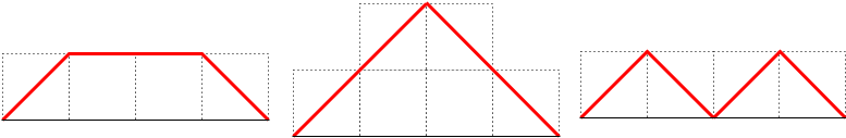
Figure 7. All three Motzkin paths in $\mathbf{M}_{0}(4)$.

If $g=0$, then $J^{\text{Planc}}_{g=0}$ is a Toeplitz matrix with spectral measure $\mu_{g=0}^{\text{Planch}}$ being the semicircle distribution. When $g\neq 0$, our Propositions 6.1, 6.8 and Theorem 6.6 imply the following.

Corollary 6.9.

If $\pm g>0$, the spectral measure $\mu_{g}^{\text{Planch}}$ of $J^{\text{Planc}}_{g}$ has discrete countable support $\operatorname{supp}(\mu^{\text{Planc}}_{g})$ with unique accumulation point $\pm\infty$. Moreover, $\mu_{g}^{\text{Planch}}$ is the unique probability measure with moments:

$$\int_{\mathbb{R}}{x^{\ell}\mu^{\text{Planc}}_{g}(dx)}=\sum_{\Gamma\in\mathbf{M}_{0}(\ell)}\prod_{i\geq 1}(i\cdot g)^{|\mathbf{S}_{\tiny\rightarrow}^{i}(\Gamma)|},\quad\forall\,\ell\in\mathbb{Z}_{\geq 1}.$$

Let $J_{g}^{\text{Planch},N}$ be the $N\times N$ truncation of $J_{g}^{\text{Planch}}$. By general theory of finite Jacobi matrices, $J_{g}^{\text{Planch},N}$ has $N$ distinct real eigenvalues $l_{1}^{(g,N)}>\cdots>l_{N}^{(g,N)}$ and there exists a unique probability measure $\mu_{g}^{\text{Planch},N}$ such that $(J_{g}^{\text{Planch},N})^{\ell}_{0,0}=\langle\mu_{g}^{\text{Planch},N},\,x^{\ell}\rangle$, for all $\ell\geq 0$. This turns out to be an atomic measure with point-masses at the eigenvalues $l_{i}^{(g,N)}$ and is called the spectral measure of $J_{g}^{\text{Planch},N}$.

Proposition 6.10.

The measures $\mu_{g}^{\text{Planch},N}$ converge weakly and in the sense of moments to $\mu_{g}^{\text{Planch}}$, as $N\to\infty$.

Proof.

For any $\ell\in\mathbb{Z}_{\geq 0}$, we have $(J_{g}^{\text{Planch}})^{\ell}_{0,0}=(J_{g}^{\text{Planch},N})^{\ell}_{0,0}$, for all large $N$. Therefore, by definition, $\mu_{g}^{\text{Planch},N}\to\mu_{g}^{\text{Planch}}$ in the sense of moments. Proposition 6.1 shows that $\mu_{g}^{\text{Planch}}$ is uniquely determined by its moments, then Theorem 3.14 implies the weak convergence. ∎

There is another point of view for the eigenvalues $l_{i}^{(g,N)}$. The orthogonal polynomials $\{H_{n}^{(g)}(x)\}_{n\geq 0}$ w.r.t. $\mu_{g}^{\text{Planch}}$ are defined by (i) $\int_{\mathbb{R}}{H_{n}^{(g)}(x)H_{m}^{(g)}(x)\mu_{g}^{\text{Planch}}(dx)}=\delta_{n,m}$, and (ii) $\deg(H_{n}^{(g)})=n$. Then it is well-known, see e.g. [Dei99, Secs. 2, 3], that the roots of the orthogonal polynomial $H_{N}^{(g)}(x)$ are real, distinct, equal to $l_{i}^{(g,N)},\,i=1,2,\cdots,N$, and the roots of $H_{N}^{(g)}(x)$ and $H_{N+1}^{(g)}(x)$ interlace.

Proposition 6.11.

$\bullet$ Assume that $g<0$. Let $l_{1}^{(g,\infty)}>l_{2}^{(g,\infty)}>\dots$ be the points of $\operatorname{supp}(\mu_{g}^{\text{Planch}})$. Then $\lim_{N\to\infty}{l_{i}^{(g,N)}}=l_{i}^{(g,\infty)}$ for each $i\in\mathbb{Z}_{\geq 1}$.

$\bullet$ Assume that $g>0$. Let $l_{1}^{(g,\infty)}<l_{2}^{(g,\infty)}<\dots$ be the points of $\operatorname{supp}(\mu_{g}^{\text{Planch}})$. Then $\lim_{N\to\infty}{l_{N+1-i}^{(g,N)}}=l_{i}^{(g,\infty)}$ for each $i\in\mathbb{Z}_{\geq 1}$.

Proof.

Fix $g<0$. We claim that for all $N,i\geq 1$, we have $\big{|}\!\operatorname{supp}(\mu_{g}^{\text{Planch},N})\cap(l_{i+1}^{(g,\infty)},l_{i}^{(g,\infty)}]\big{|}\leq 1$. Indeed, suppose that there exists $N-1\geq j\geq 1$ such that $l_{i+1}^{(g,\infty)}<l_{j+1}^{(g,N)}<l_{j}^{(g,N)}\leq l_{i}^{(g,\infty)}$. Let $H^{(g)}_{N;j}(x):=\frac{H^{(g)}_{N}(x)}{(x-l_{j}^{(g,N)})(x-l_{j+1}^{(g,N)})}$. Note that $H^{(g)}_{N;j}(x)$ is a polynomial of degree $N-2$, so that the orthogonality condition implies that $\int_{\mathbb{R}}{H_{N}^{(g)}(x)H_{N;j}^{(g)}(x)\mu_{g}^{\text{Planch}}(dx)}=0$. On the other hand, $H_{N}^{(g)}(x)H_{N;j}^{(g)}(x)=\frac{(H_{N}^{(g)}(x))^{2}}{(x-l_{j}^{(g,N)})(x-l_{j+1}^{(g,N)})}$, and for each $x\in\operatorname{supp}(\mu_{g}^{\text{Planch}})$ one has $(H_{N}^{(g)}(x))^{2}\geq 0$ and $(x-l_{j}^{(g,N)})(x-l_{j+1}^{(g,N)})\geq 0$. Since $\operatorname{supp}(\mu_{g}^{\text{Planch}})$ is infinite and discrete we conclude that $\int_{\mathbb{R}}{H_{N}^{(g)}(x)H_{N;j}^{(g)}(x)\mu_{g}^{\text{Planch}}(dx)}>0$, which gives a contradiction and proves our claim. Using a similar argument, we also have $\operatorname{supp}(\mu_{g}^{\text{Planch},N})\cap(l_{1}^{(g,\infty)},\infty)=\emptyset$.

The claim implies that for all $N\geq i\geq 1$, one has $l_{i}^{(g,N)}\leq l_{i}^{(g,\infty)}$. Since the roots of $H_{N}$ and $H_{N+1}$ interlace then for each $i\geq 1$, the sequence $(l_{i}^{(g,N)})_{N\geq 1}$ is increasing and bounded. Hence there exists a limit $\lim_{N\to\infty}l_{i}^{(g,N)}\leq l_{i}^{(g,\infty)}$. Finally, Proposition 6.10 shows that $\mu_{g}^{\text{Planch},N}$ converge weakly to $\mu_{g}^{\text{Planch}}$, as $N\to\infty$, therefore $\lim_{N\to\infty}l_{i}^{(g,N)}$ is necessarily equal to $l_{i}^{(g,\infty)}$ for each $i\geq 1$.

The case $g>0$ is analogous. ∎

Now we prove the main theorem of this section, which together with Proposition 6.11 says that the points in $\operatorname{supp}(\mu_{g}^{\text{Planch}})$, which are also the local minima of the limit profile $\omega_{g}^{\text{Planch}}=\omega_{\Lambda_{g;\,(1,0,0,\cdots)}}$, can be interpreted in two ways:

(1) as deterministic limits of the largest or smallest eigenvalues of the finite Jacobi matrices $J_{g}^{\text{Planch},N}$, and

(2) (up to certain deterministic shift) as limits in probability of the longest rows or columns of random Jack–Plancherel-distributed random partitions $\lambda^{(d)}\in\mathbb{Y}_{d}$, as $d\to\infty$.

Theorem 6.12.

Let $(\lambda^{(d)}\in\mathbb{Y}_{d})_{d\geq 1}$ be a sequence of random Young diagrams distributed by the Jack–Plancherel measures, as defined in (1) or Section 2.6.1.

$\bullet$ Assume that $g<0$. In the regime $\alpha\to 0,\,d\to\infty,\,\sqrt{\alpha d}\to-g^{-1}$, for any $i=1,2,\cdots$, we have $\,\frac{\lambda^{(d)}_{i}}{-g\cdot d}\to\lim_{N\to\infty}l_{i}^{(g,N)}-(i-1)g\,$ in probability.

$\bullet$ Assume that $g>0$. In the regime $\alpha,d\to\infty,\,\sqrt{\alpha}/\sqrt{d}\to g$, for any $i=1,2,\cdots$, we have $\,\frac{(\lambda^{(d)})^{\prime}_{i}}{-g\cdot d}\to\lim_{N\to\infty}l_{N+1-i}^{(g,N)}-(i-1)g\,$ in probability.

Proof.

Consider only $g<0$, since the case $g>0$ is analogous. We first claim that whenever $\omega_{\Lambda_{\infty}}$ has a local minimum in $z_{0}$, then it has a local maximum in $z_{0}+g$. Markov–Krein correspondence implies that the local maxima of $\omega_{\Lambda_{\infty}}$ correspond to zeroes of the Cauchy transform $G_{\mu_{g}^{\text{Planch}}}(z)$, and the local minima of $\omega_{\Lambda_{\infty}}$ correspond to poles of $G_{\mu_{g}^{\text{Planch}}}(z)$. Therefore we need to prove that if $z_{0}$ is a pole of $G_{\mu_{g}^{\text{Planch}}}(z)$, then $z_{0}+g$ is its zero. We prove the following functional equation, which immediately implies this claim:

(125) $$z\cdot G_{\mu_{g}^{\text{Planch}}}(z)-1=G_{\mu_{g}^{\text{Planch}}}(z)G_{\mu_{g}^{\text{Planch}}}(z-g).$$

By virtue of (38), both sides of (125) can be treated as formal power series in $z^{-1}$, and it is enough to prove that their coefficients are the same. Corollary 6.9 implies that both sides of (125) are $O(z^{-2})$, and for $\ell\geq 2$ the coefficient of $z^{-\ell}$ of the LHS is equal to

$$M^{\text{Planch}}_{\ell}(g):=\sum_{\Gamma\in\mathbf{M}_{0}(\ell)}\prod_{i\geq 1}(i\cdot g)^{|\mathbf{S}_{\tiny\rightarrow}^{i}(\Gamma)|}.$$

Every Motzkin path $\Gamma$ can be uniquely decomposed as the concatenation of two Motzkin paths $\Gamma=((0,0),\Gamma_{1},(k,0),\Gamma_{2})$,with $0<k\leq\ell$ and $|\mathbf{S}^{0}\big{(}((0,0),\Gamma_{1},(k,0))\big{)}|=1$. This gives

$$M^{\text{Planch}}_{0}(g)=1,\ \ M^{\text{Planch}}_{1}(g)=0,\ \ M^{\text{Planch}}_{\ell}(g)=\sum_{\ell_{1}+\ell_{2}=\ell-2}\widetilde{M}^{\text{Planch}}_{\ell_{1}}(g)\cdot M^{\text{Planch}}_{\ell_{2}}(g),\ \forall\,\ell\geq 2,$$

where $\widetilde{M}^{\text{Planch}}_{\ell}(g):=\sum_{\Gamma\in\mathbf{M}_{0}(\ell)}\prod_{i\geq 1}((i+1)\cdot g)^{|\mathbf{S}_{\tiny\rightarrow}^{i}(\Gamma)|}$. We can interpret the factor

$$\prod_{i\geq 1}((i+1)\cdot g)^{|\mathbf{S}_{\tiny\rightarrow}^{i}(\Gamma)|}=\sum_{j_{1},j_{2},\dots\in\mathbb{Z}_{\geq 0}}\,\prod_{i\geq 1}\binom{|\mathbf{S}^{i}_{\tiny\rightarrow}(\Gamma)|}{j_{i}}(i\cdot g)^{|\mathbf{S}_{\tiny\rightarrow}^{i}(\Gamma)|-j_{i}}\cdot g^{j_{i}}$$

as a sum over all subsets $S\subseteq\mathbf{S}_{\tiny\rightarrow}(\Gamma)$ of horizontal steps of $\Gamma$ and associating a standard weight $\prod_{i\geq 1}(i\cdot g)^{|\mathbf{S}_{\tiny\rightarrow}^{i}(\widetilde{\Gamma})|}$ multiplied by $g^{|S|}$ to a Motzkin path $\widetilde{\Gamma}$ obtained from $\Gamma$ by removing the horizontal steps from the chosen $S$. This interpretation allows to rewrite $\widetilde{M}^{\text{Planch}}_{\ell}(g)$:

$$\widetilde{M}^{\text{Planch}}_{\ell}(g)=\sum_{k=0}^{\ell}\binom{\ell}{k}g^{k}\cdot M^{\text{Planch}}_{\ell-k}(g)=\sum_{k=0}^{\infty}\binom{-\ell+k-1}{k}(-g)^{k}\cdot M^{\text{Planch}}_{\ell-k}(g),$$

which gives

$$M^{\text{Planch}}_{\ell}(g) =\sum_{\ell_{1},\ell_{2},k\in\mathbb{Z}_{\geq 0}\colon\atop\ell_{1}+\ell_{2}+k=\ell-2}{\!\binom{-\ell_{1}-1}{k}(-g)^{k}\cdot M^{\text{Planch}}_{\ell_{1}}(g)M^{\text{Planch}}_{\ell_{2}}(g)}$$

$$=[z^{-\ell}]G_{\mu_{g}^{\text{Planch}}}(z)G_{\mu_{g}^{\text{Planch}}}(z-g).$$

This proves the desired (125), and therefore we conclude the desired statement: if $\omega_{\Lambda_{\infty}}$ has a local minimum at $z_{0}$, then it has a local maximum at $z_{0}+g$. In particular

$$\omega_{\Lambda_{\infty}}(x)=\begin{cases}x&\text{ if }x>l_{1}^{(g,\infty)},\\ 2\,l_{i}^{(g,\infty)}-2(i-1)g-x&\text{ if }x\in[l_{i}^{(g,\infty)}+g,l_{i}^{(g,\infty)}]\text{ for some }i\geq 1,\\ x-2ig&\text{ if }x\in[l_{i+1}^{(g,\infty)},l_{i}^{(g,\infty)}+g]\text{ for some }i\geq 1.\end{cases}$$

Take any $-g>\epsilon>0$, and assume that $\epsilon\geq\|\omega_{\Lambda_{d}^{(\alpha)}}-\omega_{\Lambda_{\infty}}\|_{\infty}$. Using the same arguments as in the proof of Proposition 6.7, one can show that there exists a constant $c$ (independent of $d$) s.t. $c\epsilon\geq|(\lambda^{(d)}_{i}\cdot\frac{\sqrt{\alpha}}{\sqrt{d}}+\frac{(i-1)}{\sqrt{\alpha d}})-(l_{i}^{(g,\infty)}-2(i-1)g)|\sim|\frac{\lambda^{(d)}_{i}}{-g\cdot d}-(l_{i}^{(g,\infty)}-(i-1)g)|$. Hence, $\mathbb{P}^{(\alpha)}_{\chi_{d}}(\|\omega_{\Lambda_{d}^{(\alpha)}}-\omega_{\Lambda_{\infty}}\|_{\infty}\leq\epsilon)\leq\mathbb{P}^{(\alpha)}_{\chi_{d}}(|\frac{\lambda^{(d)}_{i}}{-g\cdot d}-(l_{i}^{(g,\infty)}-(i-1)g)|\leq c\epsilon)$ for large $d$. Theorem 2.3 shows $\lim_{d\to\infty}\mathbb{P}^{(\alpha)}_{\chi_{d}}(\|\omega_{\Lambda_{d}^{(\alpha)}}-\omega_{\Lambda_{\infty}}\|_{\infty}\leq\epsilon)=1$, therefore $\lim_{d\to\infty}{\mathbb{P}^{(\alpha)}_{\chi_{d}}(|\frac{\lambda^{(d)}_{i}}{-g\cdot d}-(l_{i}^{(g,\infty)}-(i-1)g)|\leq c\epsilon)}=1$, as desired. ∎

References

- [AB19] Gernot Akemann and Sung-Soo Byun, The high temperature crossover for general 2D Coulomb gases, J. Stat. Phys. 175 (2019), no. 6, 1043–1065. MR 3962973
- [ABG12] Romain Allez, Jean-Philippe Bouchaud, and Alice Guionnet, Invariant beta ensembles and the gauss-wigner crossover, Phys. Rev. Lett. 109 (2012), 094102.
- [BAG97] G. Ben Arous and A. Guionnet, Large deviations for Wigner’s law and Voiculescu’s non-commutative entropy, Probab. Theory Related Fields 108 (1997), no. 4, 517–542. MR 1465640
- [BC14] A. Borodin and I. Corwin, Macdonald processes, Probab. Theory Related Fields 158 (2014), no. 1-2, 225–400.
- [BD22a] Houcine Ben Dali, Generating series of non-oriented constellations and marginal sums in the Matching-Jack conjecture, Algebr. Comb. 5 (2022), no. 6, 1299–1336.
- [BD22b] by same author, Integrality in the Matching-Jack conjecture and the Farahat-Higman algebra, Preprint arXiv:2203.14879, 2022.
- [BDD23] Houcine Ben Dali and Maciej Dołęga, Positive formula for Jack polynomials, Jack characters and proof of Lassalle’s conjecture, Preprint arXiv:22305.07966, 2023.
- [BDJ99] J. Baik, P. Deift, and K. Johansson, On the distribution of the length of the longest increasing subsequence of random permutations, J. Amer. Math. Soc. 12 (1999), no. 4, 1119–1178. MR 2000e:05006
- [BDS16] Jinho Baik, Percy Deift, and Toufic Suidan, Combinatorics and random matrix theory, Graduate Studies in Mathematics, vol. 172, American Mathematical Society, Providence, RI, 2016. MR 3468920
- [BGCG22] Florent Benaych-Georges, Cesar Cuenca, and Vadim Gorin, Matrix addition and the Dunkl transform at high temperature, Comm. Math. Phys. 394 (2022), no. 2, 735–795. MR 4469406
- [BGG17] A. Borodin, V. Gorin, and A. Guionnet, Gaussian asymptotics of discrete -ensembles, Publ. Math. Inst. Hautes Études Sci. 125 (2017), 1–78. MR 3668648
- [BGP15] Florent Benaych-Georges and Sandrine Péché, Poisson statistics for matrix ensembles at large temperature, J. Stat. Phys. 161 (2015), no. 3, 633–656. MR 3406702
- [Bia98] Philippe Biane, Representations of symmetric groups and free probability, Adv. Math. 138 (1998), no. 1, 126–181. MR MR1644993 (2001b:05225)
- [Bia01] by same author, Approximate factorization and concentration for characters of symmetric groups, Internat. Math. Res. Notices (2001), no. 4, 179–192. MR MR1813797 (2002a:20017)
- [Bil95] Patrick Billingsley, Probability and measure, third ed., Wiley Series in Probability and Mathematical Statistics, John Wiley & Sons, Inc., New York, 1995, A Wiley-Interscience Publication. MR 1324786
- [BO05] Alexei Borodin and Grigori Olshanski, -measures on partitions and their scaling limits, European J. Combin. 26 (2005), no. 6, 795–834. MR 2143199
- [BO17] by same author, Representations of the infinite symmetric group, Cambridge Studies in Advanced Mathematics, vol. 160, Cambridge University Press, Cambridge, 2017. MR 3618143
- [BOO00] Alexei Borodin, Andrei Okounkov, and Grigori Olshanski, Asymptotics of Plancherel measures for symmetric groups, Journal of the American Mathematical Society 13 (2000), no. 3, 481–515.
- [CD22] Guillaume Chapuy and Maciej Dołęga, Non-orientable branched coverings, -Hurwitz numbers, and positivity for multiparametric Jack expansions, Adv. Math. 409 (2022), no. part A, Paper No. 108645, 72. MR 4477016
- [DE02] Ioana Dumitriu and Alan Edelman, Matrix models for beta ensembles, J. Math. Phys. 43 (2002), no. 11, 5830–5847. MR 1936554
- [Dei99] P. A. Deift, Orthogonal polynomials and random matrices: a Riemann-Hilbert approach, Courant Lecture Notes in Mathematics, vol. 3, New York University, Courant Institute of Mathematical Sciences, New York; American Mathematical Society, Providence, RI, 1999. MR 1677884
- [DF16] Maciej Dołęga and Valentin Féray, Gaussian fluctuations of Young diagrams and structure constants of Jack characters, Duke Math. J. 165 (2016), no. 7, 1193–1282. MR 3498866
- [DFŚ10] Maciej Dołęga, Valentin Féray, and Piotr Śniady, Explicit combinatorial interpretation of Kerov character polynomials as numbers of permutation factorizations, Adv. Math. 225 (2010), no. 1, 81–120. MR 2669350 (2011i:05267)
- [DFS14] Maciej Dołęga, Valentin Féray, and Piotr Śniady, Jack polynomials and orientability generating series of maps, Sém. Lothar. Combin. 70 (2014), Art. B70j, 50. MR 3378809
- [Doł17] Maciej Dołęga, Top degree part in -conjecture for unicellular bipartite maps, Electron. J. Combin. 24 (2017), no. 3, Paper No. 3.24, 39. MR 3691541
- [DS15] Trinh Khanh Duy and Tomoyuki Shirai, The mean spectral measures of random Jacobi matrices related to Gaussian beta ensembles, Electron. Commun. Probab. 20 (2015), no. 68, 13. MR 3407212
- [DS19] Maciej Dołęga and Piotr Śniady, Gaussian fluctuations of Jack-deformed random Young diagrams, Probab. Theory Related Fields 174 (2019), no. 1-2, 133–176. MR 3947322
- [Fér09] Valentin Féray, Combinatorial interpretation and positivity of Kerov’s character polynomials, J. Algebraic Combin. 29 (2009), no. 4, 473–507. MR MR2506718
- [For10] P.J. Forrester, Log-gases and random matrices, Princeton Univ. Press, 2010.
- [For22] Peter J. Forrester, High-low temperature dualities for the classical -ensembles, Random Matrices Theory Appl. 11 (2022), no. 4, Paper No. 2250035, 25. MR 4480830
- [FS09] Philippe Flajolet and Robert Sedgewick, Analytic combinatorics, Cambridge University Press, Cambridge, 2009. MR 2483235
- [GH19] A. Guionnet and J. Huang, Rigidity and Edge Universality of Discrete -Ensembles, Communications on Pure and Applied Mathematics 72 (2019), no. 9, 1875–1982.
- [HL21] Adrien Hardy and Gaultier Lambert, CLT for circular beta-ensembles at high temperature, J. Funct. Anal. 280 (2021), no. 7, Paper No. 108869, 40. MR 4211032
- [Hua21] Jiaoyang Huang, Law of large numbers and central limit theorems through Jack generating functions, Adv. Math. 380 (2021), Paper No. 107545, 91. MR 4200465
- [IO02] Vladimir Ivanov and Grigori Olshanski, Kerov’s central limit theorem for the Plancherel measure on Young diagrams, Symmetric functions 2001: surveys of developments and perspectives, NATO Sci. Ser. II Math. Phys. Chem., vol. 74, Kluwer Acad. Publ., Dordrecht, 2002, pp. 93–151. MR MR2059361 (2005d:05148)
- [Joh98] Kurt Johansson, On fluctuations of eigenvalues of random Hermitian matrices, Duke Math. J. 91 (1998), no. 1, 151–204. MR MR1487983 (2000m:82026)
- [Ker93] Sergei Kerov, The asymptotics of interlacing sequences and the growth of continual Young diagrams, Zap. Nauchn. Sem. S.-Peterburg. Otdel. Mat. Inst. Steklov. (POMI) 205 (1993), no. Differentsialnaya Geom. Gruppy Li i Mekh. 13, 21–29, 179. MR MR1255301
- [Ker98] by same author, Interlacing measures, Kirillov’s seminar on representation theory, Amer. Math. Soc. Transl. Ser. 2, vol. 181, Amer. Math. Soc., Providence, RI, 1998, pp. 35–83. MR MR1618739 (99h:30034)
- [Ker00] by same author, Anisotropic Young diagrams and Jack symmetric functions, Funct. Anal. Appl. 34 (2000), 41–51.
- [KO94] Sergei Kerov and Grigori Olshanski, Polynomial functions on the set of Young diagrams, C. R. Acad. Sci. Paris Sér. I Math. 319 (1994), no. 2, 121–126. MR MR1288389 (95f:05116)
- [KOO98] Sergei Kerov, Andrei Okounkov, and Grigori Olshanski, The boundary of the Young graph with Jack edge multiplicities, Internat. Math. Res. Notices (1998), no. 4, 173–199. MR 1609628
- [Las08] Michel Lassalle, A positivity conjecture for Jack polynomials, Math. Res. Lett. 15 (2008), no. 4, 661–681. MR 2424904
- [Las09] by same author, Jack polynomials and free cumulants, Adv. Math. 222 (2009), no. 6, 2227–2269. MR 2562783
- [LS77] B. F. Logan and L. A. Shepp, A variational problem for random Young tableaux, Advances in Math. 26 (1977), no. 2, 206–222. MR MR1417317 (98e:05108)
- [M1́7] Pierre-Löic Méliot, Representation theory of symmetric groups, Discrete Mathematics and its Applications (Boca Raton), CRC Press, Boca Raton, FL, 2017. MR 3616172
- [Mac95] I. G. Macdonald, Symmetric functions and Hall polynomials, second ed., Oxford Mathematical Monographs, The Clarendon Press Oxford University Press, New York, 1995, With contributions by A. Zelevinsky, Oxford Science Publications. MR 1354144
- [Mat19] K. Matveev, Macdonald-positive specializations of the algebra of symmetric functions: proof of the Kerov conjecture, Ann. of Math. (2) 189 (2019), no. 1, 277–316. MR 3898175
- [Mol23] Alexander Moll, Gaussian Asymptotics of Jack Measures on Partitions from Weighted Enumeration of Ribbon Paths, Int. Math. Res. Not. IMRN (2023), no. 3, 1801–1881, Preprint arXiv:2010.13258.
- [MP22] Pierre Mergny and Marc Potters, Rank one hciz at high temperature: interpolating between classical and free convolutions, SciPost Physics 12 (2022), no. 1, 022.
- [Nic95] Alexandru Nica, A one-parameter family of transforms, linearizing convolution laws for probability distributions, Communications in Mathematical Physics 168 (1995), 187–207.
- [NS06] Alexandru Nica and Roland Speicher, Lectures on the combinatorics of free probability, London Mathematical Society Lecture Note Series, vol. 335, Cambridge University Press, Cambridge, 2006. MR 2266879 (2008k:46198)
- [NS13] Maxim Nazarov and Evgeny Sklyanin, Integrable hierarchy of the quantum Benjamin-Ono equation, SIGMA Symmetry Integrability Geom. Methods Appl. 9 (2013), Paper 078, 14. MR 3141546
- [NT18] Fumihiko Nakano and Khanh Duy Trinh, Gaussian beta ensembles at high temperature: eigenvalue fluctuations and bulk statistics, J. Stat. Phys. 173 (2018), no. 2, 295–321. MR 3860215
- [Oko00] Andrei Okounkov, Random matrices and random permutations, Internat. Math. Res. Notices (2000), no. 20, 1043–1095. MR 1802530
- [Oko01] by same author, Infinite wedge and random partitions, Selecta Math. (N.S.) 7 (2001), no. 1, 57–81. MR MR1856553 (2002f:60019)
- [Oko03] by same author, The uses of random partitions, Fourteenth International Congress on Mathematical Physics, Word Scientists, 2003, pp. 379–403.
- [Ora05] Ferenc Oravecz, Nica’s -convolution is not positivity preserving, Communications in mathematical physics 258 (2005), no. 2, 475–478.
- [Pak20] Cambyse Pakzad, Large deviations principle for the largest eigenvalue of the Gaussian -ensemble at high temperature, J. Theoret. Probab. 33 (2020), no. 1, 428–443. MR 4064307
- [RRV11] José A. Ramírez, Brian Rider, and Bálint Virág, Beta ensembles, stochastic Airy spectrum, and a diffusion, J. Amer. Math. Soc. 24 (2011), no. 4, 919–944. MR 2813333
- [Ś19] Piotr Śniady, Asymptotics of Jack characters, J. Combin. Theory Ser. A 166 (2019), 91–143. MR 3921039
- [Śni06] Piotr Śniady, Gaussian fluctuations of characters of symmetric groups and of Young diagrams, Probab. Theory Related Fields 136 (2006), no. 2, 263–297. MR MR2240789
- [Sta89] Richard P. Stanley, Some combinatorial properties of Jack symmetric functions, Adv. Math. 77 (1989), no. 1, 76–115. MR 1014073 (90g:05020)
- [Tho64] Elmar Thoma, Die unzerlegbaren, positiv-definiten Klassenfunktionen der abzählbar unendlichen, symmetrischen Gruppe, Math. Z. 85 (1964), 40–61. MR MR0173169 (30 #3382)
- [Var58] V. S. Varadarajan, Weak convergence of measures on separable metric spaces, Sankhyā 19 (1958), 15–22. MR 94838
- [Ver74] Anatolii Moiseevich Vershik, Description of invariant measures for the actions of some infinite-dimensional groups, Doklady Akademii Nauk, vol. 218, Russian Academy of Sciences, 1974, pp. 749–752.
- [VK77] A. M. Vershik and S. V. Kerov, Asymptotic behavior of the Plancherel measure of the symmetric group and the limit form of Young tableaux, Dokl. Akad. Nauk SSSR 233 (1977), no. 6, 1024–1027. MR 0480398 (58 #562)
- [VV09] Benedek Valkó and Bálint Virág, Continuum limits of random matrices and the Brownian carousel, Invent. Math. 177 (2009), no. 3, 463–508. MR 2534097