On the Optimality of Procrastination Policy for EV charging under Net Energy Metering

Abstract

We consider the problem of behind-the-meter EV charging by a prosumer, co-optimized with rooftop solar, electric battery, and flexible consumptions such as water heaters and HVAC. Under the time-of-use net energy metering tariff with the stochastic solar production and random EV charging demand, a finite-horizon surplus-maximization problem is formulated. We show that a procrastination threshold policy that delays EV charging to the last possible moment is optimal when EV charging is co-optimized with flexible demand, and the policy thresholds can be computed easily offline. When battery storage is part of the co-optimization, it is shown that the net consumption of the prosumer is a two-threshold piecewise linear function of the behind-the-meter renewable generation under the optimal policy, and the procrastination threshold policy remains optimal, although the thresholds cannot be computed easily. We propose a simple myopic solution and demonstrate in simulations that the performance gap between the myopic policy and an oracle upper bound appears to be 0.5-7.5%.

I Introduction

We address the problem of co-optimizing behind the meter(BTM) electric vehicle (EV) charging, flexible consumptions, rooftop solar, and energy storage. This work is motivated by the increasing installation of the BTM DER and storage [1] to shift and flatten the aggregated household loads. With EV as a deferrable and interruptible load, co-optimizing BTM resources benefits not only individual prosumers but also the distribution grid operations in reduced power flow [2].

Most households with BTM DER in the U.S. are under some form of the net energy metering (NEM) tariff offered by a regulated utility or consumer choice aggregator, which bills the prosumer for its net energy consumption reading from the revenue meter, as shown in Fig. 1. Under that setting, we assume that an energy management system (EMS) controls flexible household demands, such as water heater, HVAC, EV charging, and BTM storage operations based on available renewable generations.

The co-optimization problem can be formulated as a continuous state and action space Markov decision process (MDP). Unfortunately, the solution to such a stochastic dynamic program (DP) is intractable without exploiting the special properties of the co-optimization. To this end, we focus on the particular structure of the NEM2.0 and beyond [2], where the purchasing (importing) rate is higher than the selling (exporting) rate. A striking property of such NEM tariffs is that it creates a net-zero zone in the household’s net consumption. Our work in this paper builds upon these structural properties uncovered recently in [3, 2].

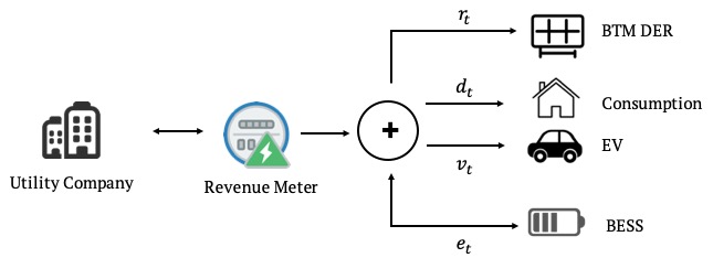
Figure 1: NEM scheme of the household with the BTM storage and EV. The direction of arrow indicates the direction of the power flow.

I-A Related works

This work is closely related to [4, 3] which studied joint scheduling of EV and flexible loads [4], and joint scheduling of ESS and flexible loads [3]. A considerable amount of research has also been conducted on the joint scheduling of BTM ESS with an EV [5, 6, 7, 8, 9, 10] and flexible demands[11, 12, 13, 14, 15], along with DER. However, only a few studies have specifically incorporated EV charging deadlines and the deferrable nature of EV into the co-optimization with storage. Moreover, to the best of our knowledge, no previous literature has explored an online scheduling of EV, storage, and consumption under NEM tariffs. In this article, we examine previous works that have investigated comparable optimization frameworks and techniques.

The co-optimization problem for the EMS with uncertainties (e.g. rooftop solar generation and outside temperature) is modeled as an one-shot optimization problem in [6, 11, 7]. However, this approach requires perfect forecasts of the uncertainties and can not provide an online policy. The authors of [6] aimed to maximize household surplus by co-optimizing flexible loads with BTM DER. In [7], the authors formulated a mixed integer linear programming (MILP) for scheduling of EV, storage, and PV power usage for the customer enrolled in a demand response program. Authors considered NEM 2.0 as the pricing tariff but they did not explicitly consider controlling household devices. In [11], MILP was formulated for the joint scheduling of controllable loads and storage with rooftop solar but EV was not considered.

Another method involves formulating co-optimization problem as an MDP and solving it using stochastic DP, which allows making online decision using the current DER generation [5, 16, 13, 14, 3, 4]. In [5], the optimal scheduling of EV and battery with rooftop solar to minimize cost and incomplete EV charging demand was studied. However, the authors did not take into account flexible demand and selling excess DER generation to the grid. In [3, 13], the authors focused on finding optimal threshold exploiting threshold structure of the optimal policy for scheduling storage and loads. Although [3, 13] did not consider EV, they are among the closely related works that studied the scheduling of loads and storage to maximize expected household surplus with surplus renewables allowed to be sold to the grid. Additionally, [4, 16] explored optimal threshold policies for the joint scheduling of deferrable and non-deferrable loads. In [14], the authors formulated stochastic control problem into Lyapunov optimization and derived closed-form scheduling of storage and loads. However, they did not consider controlling individual loads and deferrable loads such as EV.

Model predictive control (MPC) has been widely studied for joint scheduling under uncertainties as an alternate approach for solving MDP [17, 8, 9]. MPC can be adapted in real-time using the current available information but it’s performance highly depends on the forecasting algorithm, and problem size, such as look ahead horizon, and state, action space. In [8], an MPC-based joint scheduling of rooftop solar, battery, and EV that optimizes user comfort and cost was studied. Selling surplus solar generation was allowed but the selling price was the same as the energy purchasing price. In [9], the same optimization problem using MPC-based method was studied but the work included storage battery degradation cost. An MPC-based algorithm was proposed in [17] to schedule EV and flexible loads. However, the storage wasn’t scheduled, and selling to the grid was not allowed.

Recently, reinforcement learning (RL) based methods have been applied for home EMS co-optimization[18, 15, 10]. The RL-based approach has the advantage that of not requiring knowledge about uncertainties, but it is not free from the curse of dimensionality for high-dimensional discrete or continuous state/action space. For instance, [10, 18] discretized EV charging and battery operation, and applied Q-learning based method for joint scheduling of EV and loads under random price and PV generation. In [15], the authors used deep deterministic policy gradient (DDPG) algorithm for joint scheduling storage and loads in the continuous state/action space, but the algorithm converges slowly, which restricts the usage of the algorithm in an online setting.

I-B Summary of results and contributions

• We demonstrate that the procrastination threshold policy, which involves delaying EV charging to the last possible moment, which is the optimal policy for the EV, controllable loads, and DER co-optimization problem under NEM [4], is the optimal strategy for the co-optimization including myopic battery operation with the additional procrastination thresholds. Co-optimization including myopic storage operation considers battery operations with immediate stage reward and ignore future renewables and storage decisions. Additional procrastination thresholds determine the priority rule of storage operations and EV charging based on the current remaining charging demand. The procrastination thresholds, which characterize the optimal policy, can be computed offline when the BTM DER is modeled as a sequence of independent random variables. Assuming a non-binding battery SoC limit, the optimal policy for the co-optimization including non-myopic battery operations becomes myopic policy.

• The myopic storage decisions are piecewise linear function of renewable generation which is divided into 5 segments by 4 thresholds. The myopic battery operation stores energy in the battery solely using BTM DER generation, and storage discharges only to curtail the net consumption of the household.

• The empirical studies using the real-world data show that the procrastination threshold policy with myopic storage operations outperforms other non co-optimization policies and are in within 0.5-7% performance gap to an oracle policy.

The notations used in the paper are standard. Vectors are in boldface, with $(x_{1},\ldots,x_{N})$ a column vector. We use $\mathbf{1}$ for a column of ones with appropriate size. $\mathds{1}_{A}$ is an indicator function that maps to 1 if A is true, otherwise to zero.

The proofs of theorems and propositions are omitted due to space limitations, and they can be found at [19].

II Problem Formulation

We consider a sequential scheduling of EV charging $(v_{t})$, controllable household loads $(\mathbf{d}_{t})$, and storage operation $(e_{t})$ over a discrete-time and finite horizon of length $T$ with intervals indexed by $\mathcal{T}=\{0,\ldots,T-1\}$.

II-A EV charging, consumption, and storage model

BTM DER $(r_{t})$

We model the BTM DER generation during interval $t$ as an exogenous variable, represented by a sequence of independent random variables with a time-dependent distribution $f_{t}(\cdot)$. Additionally, we assume that the renewable generation for that particular interval is already known at the start of the interval.

$$r_{t}\sim f_{t}(\cdot),\quad\forall t\in\mathcal{T}$$ (1)

Remaining charging demand $(y_{t})$ and constraints

At the start of every interval, the outstanding charging demand $(y_{t})$ is measured. A charger with a maximum capacity $\bar{v}$ and charging efficiency $\eta$ provides $v_{t}$ in interval $t$. We assume that the EV does not discharge it’s battery and the total energy supplied to the EV will not exceed the amount originally requested at $t=0$ $(s_{\text{req}})$.

$$y_{t+1} =y_{t}-\eta v_{t},\quad\forall t\in\mathcal{T}.$$ (2)

$$y_{t} \in[0,s_{\text{req}}],\quad\forall t\in\mathcal{T}.$$ (3)

$$v_{t} \in[0,\min\{y_{t}/\eta,\,\bar{v}\}],\quad\forall t\in\mathcal{T}.$$ (4)

Without loss of generality we assume $\eta=1$.

Household Consumption $(\mathbf{d}_{t})$

Consumption vector $\mathbf{d}_{t}=\big{(}d_{t1},\cdots,d_{tK}\big{)}$ models the flexible consumption of $K$ controllable devices within interval $t$ which satisfy :

$$0\preceq\mathbf{d}_{t}\preceq\mathbf{\bar{d}}:=(\bar{d}_{1},\ldots,\bar{d}_{K}),\quad\forall t\in\mathcal{T}.$$ (5)

The utility $U_{t}(\mathbf{d}_{t})$ of consuming $\mathbf{d}_{t}$ is linearly separable differentiable concave function with marginal utility $L_{t}(\mathbf{d}_{t})$

$$U_{t}(\mathbf{d}_{t})=\sum_{i=1}^{K}U_{ti}(d_{ti}),\;L_{t}(\mathbf{d}_{t}):=\nabla U_{t}=\big{(}L_{t1},\ldots,L_{tK}\big{)}.$$

Our current model didn’t consider uncontrollable loads. However, this can be handled by modeling it as a sequence of independent random variables with some distribution.

Battery storage operation $(e_{t})$

The battery state of charge (SoC) is denoted as $s_{t}\in[0,B]$ where $B$ represents maximum storage capacity of the battery. Battery charging and discharging rate is denoted as $e_{t}\in[-\underline{e},\bar{e}]$, where $e_{t}\geq 0$ represents charging, and $e_{t}\leq 0$ represents discharging. Battery charging and discharging have inefficiency constants $\eta_{c}\in(0,1]$ and $\eta_{d}\in(0,1]$, respectively.

$$e_{t} \in[-\underline{e},\bar{e}],\quad\forall t\in\mathcal{T}$$ (6)

$$s_{t} \in[0,B],\quad\forall t\in\mathcal{T}$$ (7)

$$s_{t+1} =s_{t}+\eta_{c}e_{t}\mathds{1}_{e_{t}\geq 0}-\frac{e_{t}}{\eta_{d}}\mathds{1}_{e_{t}\leq 0},\quad\forall t\in\mathcal{T}.$$ (8)

Net consumption ($z_{t}$)

The net energy consumption of a household within interval $t$ is defined as the net energy measured by the revenue meter during the billing period. This includes EV charging, controllable loads, storage operation and BTM DER generation within the billing period.

$$z_{t}:=v_{t}+\mathbf{1}^{T}\mathbf{d}_{t}+e_{t}-r_{t},\quad t\in\mathcal{T}.$$

We say that household is net consuming when $z_{t}>0$, and net producing when $z_{t}<0$.

II-B NEM ToU tariff model

NEM payment $\big{(}P^{\pi_{t}}(z_{t})\big{)}$

Under the NEM tariff program, a household is billed or credited based on the net energy consumption during each billing period, which can range from 5 minutes to a day or a month. To simplify the notation, we matched the length of our decision intervals with the billing period. This enables us to index the billing period with $t$.

At interval $t$, given NEM tariff parameters $\pi_{t}=(\pi_{t}^{0},\pi_{t}^{-},\pi_{t}^{+})\in\mathbb{R}_{+}^{3}$, household with net consumption $z_{t}$ pays

$$P^{\pi_{t}}(z_{t}):=z_{t}(\mathds{1}_{z_{t}\geq 0}\pi_{t}^{+}+\mathds{1}_{z_{t}\leq 0}\pi_{t}^{-})+\pi^{0}_{t},$$

where $\pi_{t}^{+}$ is a retail rate, $\pi_{t}^{-}$ is a sell rate, and $\pi_{t}^{0}$ is a fixed charge. A prosumer pays the retail rate for the net consumption, while credited by the sell rate for the net generation. The NEM tariff model was proposed in [2]..

NEM ToU tariff model

ToU tariff divides 24 hours into periods with different energy prices. For our analysis, we adopt a ToU tariff with two distinct energy prices : off-peak and on-peak. A typical ToU tariff sets the on-peak hours to a five-hour period in the late afternoon and early evening[20]. In this work, we assume that the decision horizon falls within the first off-peak period, the on-peak period, and the second off-peak period as shown in Fig.2. Hence, once we know the connection time and the deadline, the scheduling horizon is well defined : $\mathcal{T}=\mathcal{T}_{\text{off},1}\cup\mathcal{T}_{\text{on}}\cup\mathcal{T}_{\text{off},2}$, with $T=|\mathcal{T}_{\text{off},1}|+|\mathcal{T}_{\text{on}}|+|\mathcal{T}_{\text{off},2}|$.

Figure 2: ToU scheme and decision horizon

We assume that all the intervals in the same period have the same NEM parameters and NEM parameters for every interval is known a priori. Hence,

$$\pi_{t}=\begin{cases}\pi_{\text{on}}:=(\pi_{\text{on}}^{-},\pi_{\text{on}}^{+}),&t\in\mathcal{T}_{\text{on}}.\\ \pi_{\text{off}}:=(\pi_{\text{off}}^{-},\pi_{\text{off}}^{+}),&t\in\mathcal{T}_{\text{off,1}}\cup\mathcal{T}_{\text{off,2}}.\\ \end{cases}$$ (9)

We also assume that NEM parameters satisfy $\pi_{\text{off}}^{-}<\pi_{\text{on}}^{-}<\pi_{\text{off}}^{+}<\pi_{\text{on}}^{+}$ to avoid the BTM battery is used for the price arbitrage and simplify the problem.

II-C Co-optimization of EV charging, consumption, and storage

We formulate the coordinated optimization problem into stochastic DP with state $x_{t}=(s_{t},y_{t},r_{t},\pi_{t})$. The initial SoC $(s_{0})$ and EV charging demand $(s_{\text{req}})$ is given.

The policy $\mu:=(\mu_{0},\ldots,\mu_{T-1})$ is a sequence of functions that maps the current state to EV charging, consumption and storage operation :

$$\mu_{t}(x_{t}):=(v_{t},e_{t},\mathbf{d}_{t}),\quad t\in\mathcal{T}.$$ (10)

The stage reward for the stochastic DP is the household surplus under the NEM tariff and the terminal reward is the sum of the salvage value of battery storage and the penalty for incomplete EV charging demand. The salvage value of battery storage is proportional to the terminal SoC, and the penalty for incomplete EV charging is proportional to the remaining charging demand at $t=T$.

$$g_{t}(x_{t},v_{t},e_{t},\mathbf{d}_{t}):=\begin{cases}U_{t}(\mathbf{d}_{t})-P^{\pi_{t}}(z_{t}),&t=0,\ldots,T-1.\\ \beta s_{T}-\alpha y_{T},&t=T.\end{cases}$$

Co-optimization problem is :

$$\begin{aligned} \mathcal{P}:&\max_{\mu}&&\mathbb{E}_{\mathbf{r}}\left[\sum_{t=0}^{T-1}g_{t}(x_{t},v_{t},e_{t},\mathbf{d}_{t})-\alpha y_{T}+\beta s_{T}\right]\\ &\text{s.t.}&&(1)-(10).\end{aligned}$$ (11)

We denote the optimal value function as $V_{t}(x_{t})$ that satisfies following Bellman Equation :

$$\begin{aligned} V_{t}(x_{t})&=\max_{v,e,\mathbf{d}}\;\{g_{t}(x_{t},v,e,\mathbf{d})+\mathbb{E}[V_{t+1}(x_{t+1})]\}\\ &\text{s.t. }(1)-(9)\end{aligned}$$ (12)

II-D Model Assumption

1. Price - penalty - salvage value relation : We assume that the NEM tariff parameters, the penalty for incomplete charging demand, and the battery salvage value satisfies

   $$\pi_{\text{off}}^{-}<\pi_{\text{on}}^{-}<\eta_{c}\beta<\beta/\eta_{d}<\pi_{\text{off}}^{+}<\pi_{\text{on}}^{+}<\alpha.$$

The intuition behind a high penalty for incomplete charging demand at the deadline is to allow EV charging from the BTM DER and grid purchases in all intervals, and to minimize incomplete charging demand. The penalty can be interpreted as the price of charging the EV for unfulfilled charging demand at the deadline.

An intuitive explanation for the price-salvage value relation is that 1) $\beta/\eta_{d}$ should always be greater than $\pi_{t}^{-}$ because we can always sell the energy stored in the battery to the grid at the price of $\pi_{t}^{-}$. To avoid depleting storage, it should be greater than $\pi_{t}^{-}$. 2) $\beta\eta_{c}$ should be less than $\pi_{t}^{+}$ for all $t$ because we can always purchase energy from the grid at the price of $\pi_{t}^{+}$. Consequently, to avoid the battery remaining fully charged at all time, $\beta\eta_{c}$ should be less than $\pi_{t}^{+}$.

III Procrastination threshold policy (co-optimization without battery)

We first present the procrastination threshold policy which is the optimal EV owner’s decision without a battery [4] to provide an intuition of the procrastination threshold policy. Here, $\tilde{V}_{t}$ represents the value function of the MDP without storage.

Theorem 1 (Procrastination threshold policy).

NEM ToU tariff parameters satisfying A1, and $r_{t}$ is a sequence of independent random variables, optimal EV charging $v_{t}^{*}$ and consumption $d_{t}^{*}$ decisions are monotone increasing function of $r_{t}$, and :

$$v_{t}^{*} =\begin{cases}h_{\tau_{t}}(y_{t}),&r_{t}<\Delta_{t}^{+}(y_{t})\\ h_{w_{t+1}(\nu)}(y_{t}),&\Delta_{t}^{+}(y_{t})\leq r_{t}\leq\Delta_{t}^{-}(y_{t})\\ h_{\delta_{t}}(y_{t}),&r_{t}>\Delta_{t}^{-}(y_{t}).\end{cases}$$

$$d_{ti}^{*} =\begin{cases}l_{ti}(\pi_{t}^{+}),&r_{t}<\Delta_{t}^{+}(y_{t})\\ l_{ti}(\nu),&\Delta_{t}^{+}\leq r_{t}\leq\Delta_{t}^{-}(y_{t})\\ l_{ti}(\pi_{t}^{-}),&r_{t}>\Delta_{t}^{-}(y_{t}),\end{cases}$$

$$\forall\,i=1,\ldots,K,$$

where $\nu\in[\pi_{t}^{-},\pi_{t}^{+}]$ satisfies, $r_{t}=v_{t}^{*}+\sum_{i=1}^{K}d_{ti}^{*}$.

$$\bar{V}_{t}(y) :=\mathbb{E}[\tilde{V}_{t}(y,r_{t},\pi_{t})],\quad w_{t}(\pi):=(\partial\bar{V}_{t})^{-1}(-\pi),$$

$$h_{\theta}(y) :=\min\{\bar{v},\max\{y-\theta,0\}\},$$

$$l_{ti}(\pi) :=\min\{L_{ti}^{-1}(\pi),\bar{d}_{i}\},\quad l_{t}(\pi):=\sum_{i=1}^{K}l_{ti}(\pi),$$

$$\Delta_{t}^{-}(y_{t}) :=l_{t}(\pi_{t}^{-})+h_{\delta_{t}}(y_{t})$$

$$\Delta_{t}^{+}(y_{t}) :=l_{t}(\pi_{t}^{+})+h_{\tau_{t}}(y_{t}).$$

The procrastination threshold policy at the interval $t$ is characterized by two procrastination thresholds $\tau_{t}$ and $\delta_{t}$. These thresholds represent the limit of procrastination for charging the EV. The limit of procrastination for charging EV with grid purchase is $\tau_{t}$. If $y_{t}\leq\tau_{t}$, the controller will postpone charging the EV unless there is surplus BTM DER after fulfilling consumption, as shown in Fig.3. If $y_{t}\geq\tau_{t}$, energy will be purchased from the grid to charge the EV if DER is not sufficient, but EV charging using the grid energy will not exceed $y_{t}-\tau_{t}$. On the other hand, $\delta_{t}$ represents thresholds of using DER to charge the EV. Similarly, if $y_{t}\leq\delta_{t}$, EV is not charged even if there are surplus renewables.

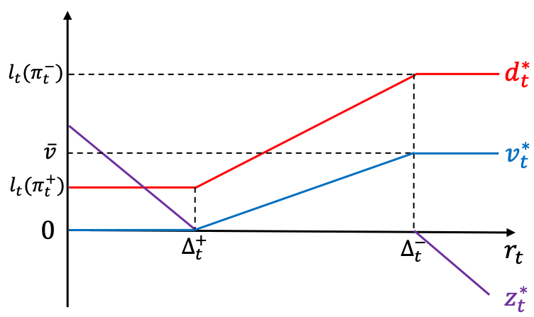
Figure 3: Procrastination threshold policy for $\delta_{t}=0<y_{t}<\tau_{t}$. In such $y_{t}$, controller will delay charging EV charging using the DER. So if renewable level is low, $r_{t}\leq\Delta_{t}^{+}$, EV is not charged, and EV is charged only when there are surplus renewables, $r_{t}\geq\Delta_{t}^{+}$.

An intuitive explanation for the optimality of procrastination charging behavior is that it increases the likelihood of completing the job using DER, which is a cheaper charging option. Let’s consider special case-a charging session with a single price-to gain insights into the policy. In this case, the limit of procrastination for purchasing energy is the maximum charging capacity of remaining intervals : $\tau_{t}=(T-t-1)\bar{v}$. Since there is no difference between purchasing at the current interval and in later intervals, it will postpone purchasing energy for charging the EV unless it’s necessary, and anticipate future renewables to complete the job with lower price.

The procrastination threshold policy is optimal if the household is either net consuming or net producing, which corresponds to the BTM DER being less than $\Delta_{t}^{+}$, and greater than $\Delta_{t}^{-}$, respectively. The optimal consumption of in these regions has the marginal value of $\pi_{t}^{+}$ and $\pi_{t}^{-}$.

In between these two thresholds, the total household load, which is the sum of EV charging and consumption, matches the current BTM DER generation, meaning the household is in the net-zero zone. In this region, BTM DER is allocated to consumption and EV charging so that the marginal utility matches the marginal reward for charging EV, $\partial\bar{V}_{t}$. The marginal reward for charging EV is the expected price of energy that can be saved by charging at the current interval.

As the utility function and NEM payment is concave, it’s easy to show that value function is also concave (Proof in the [19]). Then, the subdifferential of $\bar{V}_{t}(y)$ is non-empty, compact and monotone set. Hence, $h_{t}(\pi)$ is well defined. Also, due to the concavity of $\bar{V}_{t}(y)$ and $U_{t}(\mathbf{d})$, optimal EV charging and consumption is monotone increasing with respect to $r_{t}$ as in the Fig.3.

Following proposition shows procrastination behavior of purchasing energy to charge EV.

Proposition 1 (Procrastination charging behavior).

NEM ToU tariff parameters satisfying A1, and DER is modeled as a sequence of independent random variables, the optimal charging decisions satisfy

If $z_{t_{0}}^{*}v_{t_{0}}^{*}>0$ for $t_{0}\in\mathcal{T}_{x}$ then $v_{t}^{*}=\bar{v},\;t_{0}<\forall t\in\mathcal{T}_{x}$ ,

where $\mathcal{T}_{x}$ is $\mathcal{T}_{\mathrm{off,1}},\mathcal{T}_{\mathrm{off,2}},\mathcal{T}_{\mathrm{on}}$. ∎

This proposition implies that once the controller is purchasing energy from the grid to charge the EV, it will charge at the maximum capacity in the remaining period, as if it had reached the limit of procrastination and devoting its full capacity.

IV Optimal prosumer decisions

We now present a prosumer’s decision for EV charging, flexible loads, and storage.

IV-A Myopic co-optimization

We will use the result from the previous section and consider a co-optimization with myopic storage operations to avoid solving infinite-dimensional optimization and to unveil the structure of the policies. The battery is myopic in the sense that its storage operations ignore future storage operations and renewable generations, and immediately generate stage reward, which are the salvage values of storage. Then, the Bellman equation for the myopic co-optimization becomes :

$$V^{M}_{t}(x_{t})= \max_{v,e,\mathbf{d}}\quad g_{t}(x_{t},v,e,\mathbf{d})+\big{(}\eta_{c}\mathds{1}_{e_{t}\geq 0}-\mathds{1}_{e_{t}\leq 0}/\eta_{d}\big{)}\beta e_{t}$$ (13)

$$\quad\quad+\mathds{E}[V^{M}_{t+1}(s_{t},y_{t}-v,r_{t+1},\pi_{t+1})]$$

$$\text{s.t.}\quad-\min\{\underline{e},s_{t}\eta_{d}\}\leq e_{t}\leq\min\{\bar{e},(B-s_{t})/\eta_{c}\}$$

$$\quad\quad\;(4),(5).$$

where $V^{M}_{t}(x_{t})$ is the optimal value function for the myopic co-optimization. For the rest of the paper, we will denote the maximal charging and discharging rate constrained by SoC limit as $\underline{e}^{\prime}:=\min\{\underline{e},s_{t}\eta_{d}\}$, $\bar{e}^{\prime}=\min\{\bar{e},(B-s_{t})/\eta_{c}\}$.

Theorem 2 (Myopic optimal policy).

NEM ToU tariff parameters satisfying A1, and $r_{t}$ is a sequence of independent random variables, the optimal net consumption $z_{t}^{*}$ of myopic co-optimization (13) is a piecewise linear monotone decreasing function of $r_{t}$ :

$$z_{t}^{*}=\begin{cases}r_{t}-\Delta_{t}^{+}(y_{t}),&r_{t}<\Delta_{t}^{+}(y_{t})\\ 0,&\Delta_{t}^{+}(y_{t})\leq r_{t}\leq\Delta_{t}^{-}(y_{t})\\ r_{t}-\Delta_{t}^{-}(y_{t}),&\Delta_{t}^{-}(y_{t})<r_{t}.\end{cases}$$

The optimal EV charging $v_{t}^{*}$, consumption $d_{t}^{*}$ and the storage $e_{t}^{*}$ decisions are monotone increasing function of $r_{t}$, segmented by 6 thresholds on $r_{t}$ : $\Delta_{t}^{+}(y_{t}),\Delta_{t,1}(y_{t})-\Delta_{t,4}(y_{t}),$ and $\Delta_{t}^{-}(y_{t})$, and they are decided by Algorithm 1.

$$\Delta_{t}^{+^{\prime}}(y_{t}) :=\max\{\Delta_{t}^{+}(y_{t})-\underline{e}^{\prime},0\},$$

$$\Delta_{t,1}(y_{t}) :=\max\{l_{t}(\beta/\eta_{d})+h_{\sigma_{t}^{+}}(y_{t})-\underline{e}^{\prime},0\},$$

$$\Delta_{t,2}(y_{t}) :=l_{t}(\beta/\eta_{d})+h_{\sigma_{t}^{+}}(y_{t}),$$

$$\Delta_{t,3}(y_{t}) :=l_{t}(\beta\eta_{c})+h_{\sigma_{t}^{-}}(y_{t}),$$

$$\Delta_{t,4}(y_{t}) :=l_{t}(\beta\eta_{c})+h_{\sigma_{t}^{-}}(y_{t})+\bar{e}^{\prime},$$

$$\Delta_{t}^{-^{\prime}}(y_{t}) :=\Delta_{t}^{-}(y_{t})+\bar{e}^{\prime},$$

where $\tau_{t}>\sigma_{t}^{+}>\sigma_{t}^{-}>\delta_{t}$ for all $t\in\mathcal{T}$. ∎

If $r_{t}<\Delta_{t}^{+^{\prime}}$ and $r_{t}>\Delta_{t}^{-^{\prime}}$ (the first and the last case in Algorithm 1), the household is net consuming and net producing, and in these cases, consumption, and EV charging decisions follow procrastination threshold policy introduced in the section III.

In between these two thresholds, the household is in the net-zero zone. Here, two additional procrastination thresholds, $\sigma_{t}^{+}$ and $\sigma_{t}^{-}$, are introduced for the EV charging decisions. These thresholds determine the priority of EV charging and storage operations for allocating BTM DER. When $y_{t}<\sigma_{t}^{-}$, it implies that the remaining EV charging demand is small or deadline is still far away. Hence, priority is given to charging the storage over charging the EV. For instance, in the Fig. 4, $v_{t}^{*}>0$ when $r_{t}>\Delta_{t,4}$ and $e_{t}^{*}=\bar{e}^{\prime}$.

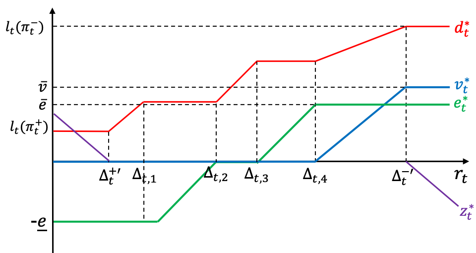
Figure 4: Myopic optimal policy for $\delta_{t}=0<y_{t}<\sigma_{t}^{-}<\sigma_{t}^{+}$. For such $y_{t}$, charging and discharging the storage is prioritized over EV charging. Hence, the EV is charged only if storage is charged to maximum, and the EV is not charged when storage is discharging.

Similarly, for $y_{t}<\sigma_{t}^{+}$, the priority is given to the discharging storage over charging the EV, which means the EV will not charge using stored energy in the BTM battery. For instance, in the Fig. 4 $v_{t}^{*}=0$ when $e_{t}^{*}<0$.

Algorithm 1 Myopic optimal decisions

$y_{t},\pi_{t},r_{t}$

$v_{t}^{*},e_{t}^{*},\mathbf{d}_{t}^{*}$

For all $i=1,\ldots,K$, myopic optimal decisions of each device are :

(with a slight abuse of notation, $\bar{V}_{t}(y):=\mathbb{E}[V_{t}^{M}(y,r_{t},\pi_{t}))]$,

$w_{t}(\pi):=(\partial\bar{V}_{t})^{-1}(-\pi)$)

if $r_{t}<\Delta_{t}^{+^{\prime}}(y_{t})$ then

     $v_{t}^{*}\leftarrow h_{\tau_{t}}(y_{t}),\quad d_{ti}^{*}\leftarrow l_{ti}(\pi_{t}^{+}),\quad e_{t}^{*}\leftarrow-\underline{e}^{\prime}$,

else if $r_{t}\in\big{[}\Delta_{t}^{+^{\prime}}(y_{t}),\Delta_{t,1}(y_{t})\big{)}$ then

     $v_{t}^{*}\leftarrow h_{w_{t+1}(\nu)}(y_{t}),\quad d_{ti}^{*}\leftarrow l_{ti}(\nu),\quad e_{t}^{*}\leftarrow-\underline{e}^{\prime}$,
where $r_{t}+\underline{e}^{\prime}=v_{t}^{*}+\sum_{i=1}^{K}d_{ti}^{*}$, and $\nu\in[\beta/\eta_{d},\pi_{t}^{+}]$,

else if $r_{t}\in\big{[}\Delta_{t,1}(y_{t}),\Delta_{t,2}(y_{t})\big{)}$ then

     $v_{t}^{*}\leftarrow h_{\sigma_{t}^{+}}(y_{t}),\quad d_{ti}^{*}\leftarrow l_{ti}(\beta/\eta_{d}),\quad e_{t}^{*}\leftarrow r_{t}-\Delta_{t,2}$,

else if $r_{t}\in\big{[}\Delta_{t,2}(y_{t}),\Delta_{t,3}(y_{t})\big{)}$ then

     $v_{t}^{*}\leftarrow h_{w_{t+1}(\nu)}(y_{t}),\quad d_{ti}^{*}\leftarrow l_{ti}(\nu),\quad e_{t}^{*}\leftarrow 0$,
where $r_{t}=v_{t}^{*}+\sum_{i=1}^{K}d_{ti}^{*}$, and $\nu\in[\beta\eta_{c},\beta/\eta_{d}]$

else if $r_{t}\in\big{[}\Delta_{t,3}(y_{t}),\Delta_{t,4}(y_{t})\big{)}$ then

     $v_{t}^{*}\leftarrow h_{\sigma_{t}^{-}}(y_{t}),\quad d_{ti}^{*}\leftarrow l_{ti}(\beta\eta_{c}),\quad e_{t}^{*}\leftarrow r_{t}-\Delta_{t,3}$,

else if $r_{t}\in\big{[}\Delta_{t,4}(y_{t}),\Delta_{t}^{-^{\prime}}(y_{t})\big{)}$ then

     $v_{t}^{*}\leftarrow h_{w_{t+1}(\nu)}(y_{t}),\quad d_{ti}^{*}\leftarrow l_{ti}(\nu),\quad e_{t}^{*}\leftarrow\bar{e}^{\prime}$,
where $r_{t}-\bar{e}^{\prime}=v_{t}^{*}+\sum_{i=1}^{K}d_{ti}^{*}$, and $\nu\in[\pi_{t}^{-},\beta\eta_{c}]$

else

     $v_{t}^{*}\leftarrow h_{\delta_{t}}(y_{t}),\quad d_{ti}^{*}\leftarrow l_{ti}(\pi_{t}^{-}),\quad e_{t}^{*}\leftarrow\bar{e}^{\prime}$

end if

In the net-zero zone, either the total household load (sum of consumption and EV charging) or storage operation increases with renewables. When, the battery operation is a constant function of $r_{t}$ (case 2, 4, and 6 in Algorithm 1), the total household load matches $r_{t}-e_{t}$, BTM DER adjusted by storage output. For instance, if $r_{t}\in\big{[}\Delta_{t}^{+^{\prime}}(y_{t}),\Delta_{t,1}(y_{t})\big{)}$, the total household load matches sum of BTM DER and maximal storage discharging. The storage output adjusted renewables are allocated as the net-zero zone decisions of the co-optimization without storage.

One thing to note that, by introducing the storage, the household has a wider net zero zone compared to the co-optimization without storage. This implies increased internal usage of BTM DER within the household.

The optimal myopic storage operation is a piecewise linear function and it shows a complementarity property with the total household load, which is defined as $e_{t}^{*}z_{t}^{*}\leq 0$ [3]. This implies that energy is stored in the battery only using the BTM DER, and storage only discharges to reduce net consumption. This result is intuitive because, from A1, $\pi^{-}<\beta\eta_{c}<\pi^{+}$, so storage charging is beneficial only when using the BTM DER. Also, as $\pi^{-}<\beta/\eta_{d}<\pi^{+}$, discharging stored energy in the battery is beneficial only if it is used to reduce the net load.

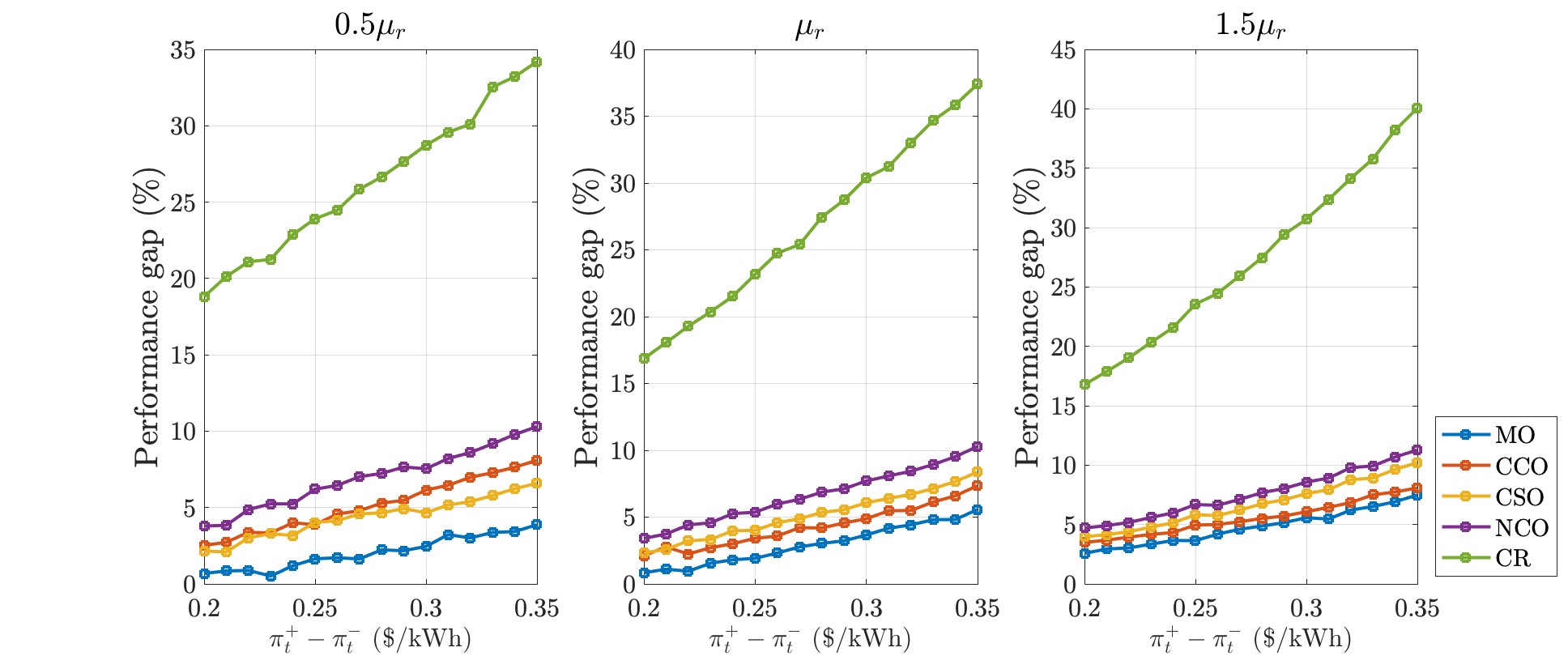
Figure 5: Relative performance gap of the MO(blue), CCO(red), CSO(yellow), NCO(purple), CR(green) to the oracle policy for different $\pi_{t}^{+}-\pi_{t}^{-}$ is plotted. The estimated mean of renewable is scaled by 0.5, 1, 1.5 for the figures from left to right.

IV-B Co-optimization with non-binding SoC assumption

Now, we make the following additional assumption on the battery SoC limit :

1. Non-binding battery SoC limit : Battery SoC limit constraint, (7), is non binding for all $t\in\mathcal{T}$.

This assumption is restrictive but it can be valid if the storage capacity is large relative to the maximum storage charging and discharging rate, or if the maximum charging and discharging rate is relatively low. Under assumption A2, we can show that the optimal policy for the stochastic co-optimization problem (11) becomes myopic.

Theorem 3 (Optimal prosumer decisions).

Under A1-A2, and BTM DER modeled as a sequence of independent random variables, optimal battery, consumption, EV charging decisions of Theorem 2 is the optimal solution of the problem (11).

IV-C Computation of the thresholds

We now comment on the computation of the thresholds that characterize the myopic optimal policy. The renewable thresholds, $\Delta_{t}$’s, are comprised of thresholds on consumption and EV charging. Flexible loads are not coupled between time, hence given consumer utility function, NEM parameter, and storage parameters, we can compute the consumption thresholds offline.

The following proposition presents the characterization of procrastination thresholds.

Proposition 2 (Characterization of procrastination thresholds).

NEM ToU tariff parameters satisfying A1, and DER is modeled as a sequence of independent random variables, the optimal procrastination thresholds $\tau_{t},\sigma_{t}^{+},\sigma_{t}^{-},\delta_{t}$ satisfy :

$$\tau_{t} =\begin{cases}(T-t-1)\bar{v},&t\in\mathcal{T}_{\mathrm{off,2}}\cup\mathcal{T}_{\mathrm{on}}\\ w_{t+1}(\pi_{\mathrm{off}}^{+}),&t\in\mathcal{T}_{\mathrm{off,1}}\end{cases}$$

$$\delta_{t} =\begin{cases}\raisebox{-6.88889pt}{$0$,}&t\in\mathcal{T}_{\mathrm{off,1}}\cup\mathcal{T}_{\mathrm{off,2}},\\ &t\in\mathcal{T}_{\mathrm{on}}\land\mathcal{T}_{\mathrm{off,2}}=\emptyset\\ w_{t+1}(\pi_{\mathrm{on}}^{-}),&t\in\mathcal{T}_{\mathrm{on}}\land\mathcal{T}_{\mathrm{off,2}}\neq\emptyset\end{cases}$$

$$\sigma_{t}^{+} =w_{t+1}(\beta/\eta_{d})$$

$$\sigma_{t}^{-} =w_{t+1}(\beta\eta_{c})$$

$\tau_{t}$ and $\delta_{t}$ satisfy following recursive relation within same pricing period :

$$\tau_{t} =\tau_{t+1}+\bar{v},$$

$$\delta_{t} =\delta_{t+1}.$$

In intervals with the purchasing procrastination threshold $\tau_{t}=(T-t-1)\bar{v}$, energy is purchased for charging EV only if it’s necessary to meet the charging requirement by the deadline. Combining the result of Proposition 1-2, the procrastination threshold policy always guarantees completion of the charging requirement by the deadline whenever it’s possible $(s_{\text{req}}\leq T\bar{v})$.

Other thresholds that involve $w_{t+1}(\cdot)$ can be computed offline by solving dynamic programming equations. Such procrastination thresholds depend on the distribution of future renewable generation, and represent value of $y_{t}$ such that expected value of charging is equal to the argument of $w_{t+1}(\cdot)$.

V Numerical results

We implemented numerical simulations using real-world data, which involve a household with the BTM storage and EV under the utility’s NEM tariff, to verify the performance of the myopic optimal policy presented in this paper and demonstrate the benefits of co-optimization.

We compared the performance of different policies using the relative expected accumulated surplus gap to the oracle policy. The oracle policy is the offline policy which is the outcome of solving convex optimization (11) with the realization of renewables, which will serve as the upper bound of the performance. If the oracle policy and comparing policy’s expected accumulated reward is $R_{OR}$, and $R_{\mu}$, respectively, the performance measure of the policy is

$$\frac{R_{OR}-R_{\mu}}{R_{OR}}.$$

The myopic optimal policy (MO) in Theorem 2 is compared with 4 different policies with different level of co-optimization. The policies we considered are :

1. Cost reduction policy (CR)

2. Non co-optimization policy (NCO)

3. Consumption-storage co-optimized policy (CSO)

4. Charging-consumption co-optimized policy (CCO)

Policies are listed in the order of increasing levels of co-optimization. CR uses renewables and storage to reduce the costs, with the EV primarily charges in off-peak periods, while consumption is not optimized. NCO and CSO optimize the EV first, while NCO optimizes each device separately in the order of EV, consumption, and storage. CSO co-optimizes consumption and storage. CCO co-optimizes consumption and EV charging as Theorem 1, and then optimizes storage. Essentially, all the policies use the battery to reduce the cost and store surplus renewables.

V-A Simulation setting

We implemented Monte Carlo simulations with random EV charging demand, BTM DER trajectory, and connection time. The distribution of EV charging demand was modeled using the charging request data from Adaptive Charging Network [21]. To model the distribution of rooftop solar generation, we used New York residential solar generation data from the Pecan Street [22]. Lastly, we assumed that the connection time of the EV is equally distributed.

For the NEM ToU tariff parameters, we used the ToU retail rate from the Pacific Gas and Electronic (PG&E) with on-peak hours from 4 PM to 9 PM. The sell rate was selected as a parameter to vary.

The BTM storage has a maximum capacity of $B=13.5$ kWh and we assumed that $s_{0}=0.5B$. The maximum charging and discharging rate are $\bar{e}=\underline{e}=3.2$kW, and the charging/discharging inefficiency constants are $\eta_{c}=\eta_{d}=0.95$. The chosen salvage value of storage, $\beta$, satisfies $A1$.

In our simulation, we considered a household with a single controllable load, modeling total consumption of the household. We adopted a quadratic concave utility function that has the form $U(d)=ad-1/2bd^{2}$. The coefficients of the utility function were estimated based on the consumption data from Pecan Street, and the ToU retail rate.

As mentioned earlier, the EV charger has an efficiency of 1 and the maximum charging capacity is 3.6 kW.

V-B Performance of myopic optimal policy

We present the simulation results of 100,000 Monte Carlo runs that show the performance gap of different policies when the retail rate is fixed and the sell rate is varied, assuming that $\pi_{t}^{+}-\pi_{t}^{-}$ is kept constant at all intervals. The decision horizon $T$ is fixed as 16 hours. The three different plots in Fig.5 show the relative surplus gap when the mean of the distribution of DER generation is scaled by 0.5, 1, 1.5 from left to right.

In the plots, we can observe that the MO has the smallest gap with the oracle policy ranging from 0.5-7.5% in all scenarios. This result shows the value of co-optimization. The performance gap increases as the mean of the renewable increases, because with a higher renewable level, more renewables will be stored in the battery, and it is more likely that the non-binding SoC limit assumption will be violated.

When $\pi_{t}^{-}$ is lowered, the performance gap of MO is increasing. For instance, for 50% renewable means case, performance gap is increased from 0.6% to 3.8%. A low sell rate means that BTM DER generation has low value when it’s exported to the grid. It also implies using renewable internally is cheaper in terms of opportunity cost. Hence, to complete charging requirement of EV using the renewables, procrastination thresholds $(\tau_{t},\sigma_{t}^{+},\sigma_{t}^{-})$ are increased. This procrastinating behavior allocates more renewables to the storage, increasing the likelihood of violating the SoC limit non-binding assumption.

We can also observe that the gap with MO to other policies (CCO, CSO, NCO) are shrinking as the mean of the renewable distribution increases. The biggest gap between MO and NCO is reduced from 6.4% for the 50% renewable mean case to 1.9% for 150% renewable mean case. When the renewable level is high, the decisions of co-optimization policy get closer to the decisions of non co-optimization policies because there are sufficient renewables to be used for all devices. Hence, this result implies that the value of co-optimization is maximized when renewable level is low.

VI Conclusion

This paper has presented a comprehensive analysis of co-optimizing BTM DER with storage, EV charging and controllable loads under NEM tariff. Our results suggest that under the NEM tariff, procrastination threshold policy for EV charging and myopic storage operations provide economic benefit to the household. Furthermore, the thresholds that characterize the procrastination threshold policy can be computed offline and the policy can be easily implemented in real-time.

It should be noted that the scope of this study was limited to co-optimizing a single EV with BTM DER and storage, and as such, application of our work to commercial or industrial EMS settings, which can have multiple EVs, is not trivial. There reside priority rules of different EVs, and high dimensionality of the control space can complicate the problem. This problem can be studied in future works. Also, our work assumes that we have information on the consumer utility and the BTM DER distribution. Model-free reinforcement learning approach using the structure of the proposed policy can be studied in the future works to avoid modeling of unknown utility function and BTM DER generation distributions.

Appendix A Proofs

The optimality of procrastination threshold policy for the co-optimization without storage (Theorem 1) was proved [4]. We will prove the Proposition 1 which wasn’t stated in [4].

A-A Proof of Proposition 1

Proof.

By the proposition 2 in [4], $\tau_{t}$ and $\tau_{t+1}$ satisfy :

$$\tau_{t}=\tau_{t+1}+\bar{v}$$

For some $t_{0}\in\mathcal{T}_{x}$, given $y_{t_{0}}$, if $z_{t_{0}}^{*}v_{t_{0}}^{*}>0$, by the procrastination threshold policy, $y_{t_{0}}>\tau_{t_{0}}$ and,

$$v_{t_{0}}^{*}=\min\{\bar{v},y_{t_{0}}-\tau_{t_{0}}\}.$$

Then, $y_{t_{0}+1}=y_{t_{0}}-v_{t_{0}}^{*}\geq\tau_{t_{0}}=\tau_{t_{0}+1}+\bar{v}.$ Hence, by the monotonicity of $v_{t}^{*}$ with respect to $r_{t}$, $v_{t_{0}+1}^{*}=\bar{v}$ for all $r_{t_{0}+1}$.

The recursive relation of $\tau_{t}$ holds within the same period, therefore, $v_{t}^{*}=\bar{v}$ for all $t\in\mathcal{T}_{0}$ such that $t>t_{0}$. ∎

A-B Concavity of the optimal value function

We first prove the concavity of the optimal value function of myopic co-optimization. Here, we are only interested in concavity of the value function with respect to $y_{t}$. So, let’s simplify the notation as $V_{t}^{M}(y_{t})$.

Lemma 1.

Optimal value function of myopic co-optimization, $V_{t}^{M}(y_{t})$, that satisfies Bellman equation (LABEL:eq:myopic_opt) is concave function of $y_{t}$.

Proof.

At $t=T-1$, there is no uncertainty and Bellman equation becomes

$$V_{T-1}^{M}(y_{T-1}) =\max_{v,e,\mathbf{d}}\,\{g_{T-1}(x_{T-1},v,e,\mathbf{d})-\alpha(y_{T-1}-v)$$

$$\quad+\beta(\mathbbm{1}_{e\geq 0}\eta_{c}-\mathbbm{1}_{e\leq 0}/\eta_{d})(s_{T-1}+e)\}$$

$$\text{s.t.}\quad(4)-(5)$$

As $\alpha>\pi^{+}>\pi^{-}$, the optimal EV charging action is

$$v^{*}=\min\{\bar{v},y_{T-1}\}.$$

For $y_{T-1}>\bar{v}$, optimal consumption and storage operation are independent to $y_{T-1}$ and $\frac{\partial}{\partial y_{T-1}}V^{M}_{T-1}=-\alpha$.

For $y_{T-1}\leq\bar{v}$, optimal consumtion and storage operation is decided based on the remaining renewables $\tilde{r}_{T-1}=\max\{r_{T-1}-y_{T-1},0\}$. Consumption-storage co-optimization decision is based on myopic co-optimization in [3].

If household is net consuming, $\tilde{r}_{T-1}\leq l_{T-1}(\pi_{T-1}^{+})-\underline{e}^{\prime}$, $\frac{\partial}{\partial y_{T-1}}V^{M}_{T-1}=-\pi_{T-1}^{+}<-\alpha$.

As $y_{T-1}$ reduces, $\tilde{r}_{T-1}$ increases, and household will be in the net zero zone. In the net zero zone, $\frac{\partial}{\partial y_{T-1}}V^{M}_{T-1}$ is the negative of marginal utility of consumption, and as the consumption is increasing, marginal utility decreases. Therefore, $\frac{\partial}{\partial y_{T-1}}V^{M}_{T-1}$ increases. At last, household enters, net producing region, which means $\frac{\partial}{\partial y_{T-1}}V^{M}_{T-1}=-\pi_{T-1}^{-}$.

Hence, $\frac{\partial}{\partial y_{T-1}}V^{M}_{T-1}$ is a decreasing function of $y_{T-1}$, therefore, $V^{M}_{T-1}(x_{T-1})$ is a concave function of $y_{T-1}$.

Suppose, $V^{M}_{t+1}$ is a concave function of $y_{t+1}$. Then, the objective function of bellman equation is concave and continuous in the compact feasible set, there exists a optimal solution for every $y_{t}$. Let’s denote the optimal solution for $y_{t}=\kappa,$ as $v_{\kappa}^{*},e_{\kappa}^{*},\mathbf{d}_{\kappa}^{*}$, and for $y_{t}=\zeta$ as $v_{\zeta}^{*},e_{\zeta}^{*},\mathbf{d}_{\zeta}^{*}$.

$$\lambda V_{t}^{M}(\kappa) +(1-\lambda)V_{t}^{M}(\zeta)$$

$$=\lambda\{g_{t}(\kappa,v_{\kappa}^{*},e_{\kappa}^{*},\mathbf{d}_{\kappa}^{*})+\mathbb{E}[V_{t+1}^{M}(\kappa-v_{\kappa}^{*})]\}$$

$$+(1-\lambda)\{g_{t}(\zeta,v_{\zeta}^{*},e_{\zeta}^{*},\mathbf{d}_{\zeta}^{*})+\mathbb{E}[V_{t+1}^{M}(\zeta-v_{\zeta}^{*})\}$$

$$\leq g_{t}(\xi,v_{\xi},e_{\xi},\mathbf{d}_{\xi})+\mathbb{E}[V_{t+1}^{M}(\xi-v_{\xi})]$$

$$\leq g_{t}(\xi,v_{\xi}^{*},e_{\xi}^{*},\mathbf{d}_{\xi}^{*})+\mathbb{E}[V_{t+1}^{M}(\xi-v_{\xi}^{*})]$$

$$=V_{t}^{M}(\xi)=V_{t}^{M}(\lambda\kappa+(1-\lambda)\zeta)$$

Here, $\xi=\lambda\kappa+(1-\lambda)\zeta$, $v_{\xi}=\lambda v_{\kappa}^{*}+(1-\lambda)v_{\xi}^{*}$, $e_{\xi}=\lambda e_{\kappa}^{*}+(1-\lambda)e_{\xi}^{*}$, $\mathbf{d}_{\xi}=\lambda\mathbf{d}_{\kappa}^{*}+(1-\lambda)\mathbf{d}_{\xi}^{*}$.

The first inequality holds, because of the concavity of the stage reward function of inductive hypothesis.

Hence, $V_{t}^{M}$ is a concave function of $y_{t}$ for all $t\in\mathcal{T}$. ∎

A-C Storage operation propositions

For the rest of the proofs, $d_{t}^{*}=\mathbf{1}^{T}\mathbf{d}_{t}^{*}$. The proof of the following propositions are shown in [3]

Proposition 3 (Storage salvage value under non-binding SoC assumption).

Under assumption A1 and A2, for $\epsilon>0$ that doesn’t violate non-binding SoC assumption,

$$V_{t}(s_{t}+\epsilon,y_{t},r_{t}) =V_{t}(s_{t},y_{t},r_{t})+\beta\eta_{c}\epsilon$$

$$V_{t}(s_{t}-\epsilon,y_{t},r_{t}) =V_{t}(s_{t},y_{t},r_{t})-\beta/\eta_{d}\epsilon$$

Proposition 4 (Storage-total load complementarity condition).

Under A1-A2, optimal storage operations and net consumption of the myopic co-optimization (LABEL:eq:myopic_opt) satisfy

$$e_{t}^{*}z_{t}^{*}\leq 0,$$

$$e_{t}^{*}(d_{t}^{*}+v_{t}^{*}-r_{t})\leq 0.$$

Proposition 5 (Optimal storage operation).

Under A1-A2, for all $t\in\mathcal{T}$, for the optimal consumption $\mathbf{d}_{t}^{*}$ and EV charging $v_{t}^{*}$ of (LABEL:eq:myopic_opt), $e_{t}^{*}$ satisfies

$$e^{*}_{t}=\begin{cases}\max\{r_{t}-d_{t}^{*}-v_{t},-\underline{e}^{\prime}\},&r_{t}\leq d_{t}^{*}+v_{t}^{*}\\ \min\{r_{t}-d_{t}^{*}-v_{t},\bar{e}^{\prime}\},&r_{t}>d_{t}^{*}+v_{t}^{*}\end{cases}$$

and $e_{t}^{*}\leq r_{t}$.

A-D Proof of Theorem 2

Proof.

Let’s consider three regions of $r_{t}$ divided by $\Delta_{t}^{+^{\prime}}$ and $\Delta_{t}^{-^{\prime}}$.

1. $r_{t}<\Delta_{t}^{+^{\prime}}(y_{t})$ : Define storage output augmented renewable $\tilde{r}_{t}:=r_{t}-e_{t}^{*}$. Then, by Proposition 5, and $e_{t}^{*}\geq-\underline{e}^{\prime}$,

   $$0<\tilde{r}_{t}<l_{t}(\pi_{t}^{+})+h_{\tau_{t}}(y_{t})$$

   Hence, by Theorem 1,

   $$v_{t}^{*}=h_{\tau_{t}}(y_{t}),\,d_{ti}^{*}=l_{ti}(\pi_{t}^{+}),\;\forall i=1,\ldots,K.$$

   Then, $v_{t}^{*}+d_{t}^{*}>r_{t}$, and $e_{t}^{*}=-\underline{e}^{\prime}$. Therefore,

   $$z_{t}^{*}=v_{t}^{*}+d_{t}^{*}+e_{t}^{*}-r_{t}=\Delta_{t}^{+^{\prime}}(y_{t})-r_{t}$$

2. $r_{t}>\Delta_{t}^{-^{\prime}}(y_{t})$ : For such $r_{t}$, storage output augmented renewable satisfies

   $$\tilde{r}_{t}=r_{t}-e_{t}^{*}>l_{t}(\pi_{t}^{-})+h_{\delta_{t}}(y_{t})$$

   Then, by Theorem 1,

   $$v_{t}^{*}=h_{\delta_{t}}(y_{t}),\,d_{ti}^{*}=l_{ti}(\pi_{t}^{-}),\;\forall i=1,\ldots,K.$$

   From Proposition 5, as $v_{t}^{*}+d_{t}^{*}<r_{t}$, $e_{t}^{*}=\bar{e}^{\prime}$. Therefore,

   $$z_{t}^{*}=v_{t}^{*}+d_{t}^{*}+e_{t}^{*}-r_{t}=\Delta_{t}^{-^{\prime}}(y_{t})-r_{t}$$

3. $r_{t}\in[\Delta_{t}^{+^{\prime}}(y_{t}),\Delta_{t}^{-^{\prime}}(y_{t})]$ : Note that $z_{t}^{*}=0$ for $r_{t}=\Delta_{t}^{+^{\prime}}(y_{t})$ and $r_{t}=\Delta_{t}^{-^{\prime}}(y_{t})$. Hence, it’s suffice to show that $z_{t}^{*}$ is a monotone decreasing function of $r_{t}$ in this region.
   

   For $r_{t}=\Delta_{t}^{+^{\prime}}(y_{t})$, and $\epsilon>0$ such that $r_{t}+\epsilon\in[\Delta_{t}^{+^{\prime}}(y_{t}),\Delta_{t}^{-^{\prime}}(y_{t})]$, suppose optimal net consumption of $r_{t}+\epsilon$ is $\tilde{z}_{t}^{*}>0$. Let’s denote the optimal scheduling of each device as $\tilde{v}_{t}^{*},\,\tilde{\mathbf{d}}_{t}^{*},\,\tilde{e}_{t}^{*}$. By Proposition 5, $\tilde{e}_{t}^{*}=-\underline{e}^{\prime}$.

   $$r_{t}+\epsilon-\tilde{e}_{t}^{*}=r_{t}+\epsilon+\underline{e}^{\prime}\geq r_{t}-e_{t}^{*}=l_{t}(\pi_{t}^{+})+h_{\delta_{t}}(y_{t})=\Delta_{t}^{+}(y_{t})$$

   The first inequality holds because $e_{t}^{*}\geq-\underline{e}^{\prime}$. The second equality comes from Theorem 1.
   

   By Theorem 1, if $r_{t}+\epsilon-\tilde{e}_{t}^{*}\geq\Delta_{t}^{+}(y_{t})$, $\tilde{v}_{t}^{*}+\tilde{\mathbf{d}}_{t}^{*}\leq r_{t}+\epsilon-\tilde{e}_{t}^{*}$. Hence, $\tilde{z}_{t}^{*}\leq 0$ which contradicts the assumption. Therefore, $z_{t}^{*}$ is a monotone decreasing function with respect to $r_{t}$.

Now let’s show that $v_{t}^{*},d_{t}^{*},e_{t}^{*}$ are determined by Algorithm 1. From the proof of optimal net consumption, we proved optimal myopic decision for $r_{t}<\Delta_{t}^{+^{\prime}}(y_{t})$ and $r+t>\Delta_{t}^{-^{\prime}}(y_{t})$. Let’s prove the myopic optimal schedule in the net-zero zone. In this region, myopic co-optimization becomes,

$$\max_{v,e,\mathbf{d}} U_{t}(\mathbf{d})+\big{(}\eta_{c}\mathbbm{1}_{e_{t}\geq 0}-\mathbbm{1}_{e_{t}\leq 0}/\eta_{d}\big{)}\beta e_{t}$$

$$+\mathbbm{E}[V^{M}_{t+1}(s_{t},y_{t}-v,r_{t+1},\pi_{t+1})]$$

s.t. $$-\underline{e}^{\prime}\leq e_{t}\leq\bar{e}^{\prime} (\bar{\lambda}_{e},\underline{\lambda}_{e})$$

$$0\preceq\mathbf{d}\preceq\bar{\mathbf{d}} (\boldsymbol{\bar{\lambda}}_{d},\boldsymbol{\underline{\lambda}}_{d})$$

$$0\leq v\leq\bar{v} (\bar{\lambda}_{v},\underline{\lambda}_{v})$$

$$v+\mathbf{1}^{T}\mathbf{d}+e=r (\nu)$$

Here, $(\bar{\lambda}_{e},\underline{\lambda}_{e}),\,(\boldsymbol{\bar{\lambda}}_{d},\boldsymbol{\underline{\lambda}}_{d}),\,(\bar{\lambda}_{v},\underline{\lambda}_{v})$ are the Lagrange multipliers for the corresponding constraints.

Lagrangian of the optimization problem is

$$\mathcal{L} =U(\mathbf{d})+\mathbbm{E}[V^{M}_{t+1}(s_{t},y_{t}-v,r_{t+1},\pi_{t+1})]$$

$$+\big{(}\eta_{c}\mathbbm{1}_{e_{t}\geq 0}-\mathbbm{1}_{e_{t}\leq 0}/\eta_{d}\big{)}\beta e_{t}+\underline{\lambda}_{e}(e_{t}+\underline{e}^{\prime})+\bar{\lambda}_{e}(\bar{e}^{\prime}-e_{t})$$

$$+\boldsymbol{\underline{\lambda}}_{d}^{T}\mathbf{d}+\boldsymbol{\bar{\lambda}}_{d}^{T}(\mathbf{\bar{d}}-\mathbf{d})+\underline{\lambda}_{v}v+\bar{\lambda}_{v}(\bar{v}-v)$$

$$+\nu(v+\mathbf{1}^{T}\mathbf{d}+e-r)$$

As above optimization satisfies Slater’s condition, KKT condition becomes necessary and sufficient condition. Let’s verify myopic optimal decisions in Algorithm 1 satisfies KKT condition.

1. $r_{t}\in\big{[}\Delta_{t}^{+^{\prime}}(y_{t}),\Delta_{t,1}(y_{t})\big{)}:$ By complementary slackness, $\underline{\lambda}_{e}=0$. Then, $\nu=\beta/\eta_{d}+\bar{\lambda}_{e}$.
   

   $\tilde{r}_{t}=r_{t}+\underline{e}^{\prime}\in[\Delta_{t}^{+}(y_{t}),l_{t}(\beta/\eta_{d})+h_{\sigma_{t}^{+}}(y_{t}))$. Hence, from Theorem 1, optimal EV charging and consumption decisions are

   $$v_{t}^{*}=h_{w_{t+1}(\nu)}(y_{t}),\,d_{ti}^{*}=l_{ti}(\nu),\,\forall i=1,\ldots,K$$

   where $\nu\in[\pi_{t}^{+},\beta/\eta_{d})$. Here, due to the monotonicity of $L_{t}$ and $\partial(\bar{V}_{t})$, $v_{t}^{*}$ and $d_{t}^{*}$ are monotone increasing with respect to $r_{t}$.

2. $r_{t}\in\big{[}\Delta_{t,1}(y_{t}),\Delta_{t,2}(y_{t})\big{)}$ : By complementary slackness, $\bar{\lambda}_{e}=\underline{\lambda}_{e}=0$. Hence, $\nu=\beta/\eta_{d}$. Then, by the stationarity condition, optimal EV charging and consumption decisions are

   $$v_{t}^{*}=h_{\sigma_{t}^{+}}(y_{t}),\,d_{ti}^{*}=l_{ti}(\beta/\eta_{d}),\,\forall i=1,\ldots,K,$$

   where $\sigma_{t}^{+}=w_{t+1}(\beta/\eta_{d})$. By monotonicity of $L_{t}$ and $\partial(\bar{V}_{t})$, optimal EV charging and consumption decisions are no less than the optimal EV charging and consumption decisions of previous case, respectively. Hence, montonicity of myopic optimal policy still holds.

3. $r_{t}\in\big{[}\Delta_{t,2}(y_{t}),\Delta_{t,3}(y_{t})\big{)}$ : As $e_{t}^{*}=0$, by complementary slackness, $\bar{\lambda}_{e}=\underline{\lambda}_{e}=0$. From Theorem 1, optimal EV charging and consumption decisions are

   $$v_{t}^{*}=h_{w_{t+1}}(y_{t}),\,d_{ti}^{*}=l_{ti}(\nu),\;\forall i=1,\ldots,K$$

   where $\nu\in[\beta\eta_{c},\beta/\eta_{d}]$ and $v_{t}^{*}+d_{t}^{*}=r_{t}$. Similarly, monotonicity of $v_{t}^{*}$ and $d_{t}^{*}$ holds due to monotonicity of $L_{ti}$ and $\partial(\bar{V}_{t})$.

4. $r_{t}\in\big{[}\Delta_{t,3}(y_{t}),\Delta_{t,4}(y_{t})\big{)}$ : By complementary slackness, $\bar{\lambda}_{e}=\underline{\lambda}_{e}=0$ and $\nu=\eta_{c}\beta$. By stationarity condition, optimal EV charging and consumption decisions are

   $$v_{t}^{*}=h_{\sigma_{t}^{-}}(y_{t}),\,d_{ti}^{*}=l_{ti}(\beta/\eta_{d}),\,\forall i=1,\ldots,K,$$

   where $\sigma_{t}^{-}=w_{t+1}(\beta\eta_{c})$. Montonicity of the optimal decisions still holds.

5. $r_{t}\in\big{[}\Delta_{t,4}(y_{t}),\Delta_{t}(y_{t})^{-^{\prime}}\big{)}$ : By complemenatry slackness, $\bar{\lambda}_{e}=0$. Then, $\nu=\beta\eta_{c}+\underline{\lambda}_{e}$.

   For $\tilde{r}_{t}=r_{t}-\bar{e}^{\prime}\in\big{[}l_{t}(\beta\eta_{c})+h_{\sigma_{t}^{-}}(y_{t}),\Delta_{t}^{-}(y_{t})\big{)}$, by Theorem 1, optimal EV charging and consumption decisions are

   $$v_{t}^{*}=h_{w_{t+1}}(y_{t}),\,d_{ti}^{*}=l_{ti}(\nu),\;\forall i=1,\ldots,K,$$

   where $\nu\in[\beta\eta_{c},\pi_{t}^{-}]$.

Overall, monotonicity of $v_{t}^{*},\,d_{t}^{*}$ holds due to the monotonicity of $l_{ti}$ and $\partial(\bar{V}_{t})$. ∎

A-E Proof of Theorem 3

Proof.

It’s suffice to show that for $s_{t}$ that satisfies A2 and $\boldsymbol{\gamma}=(\epsilon,0,0,0)$ ($\epsilon>0$), optimal value function that satisfies (12), satisfies

$$V_{t}(x_{t}+\boldsymbol{\gamma}) =V_{t}(x_{t})+\beta\epsilon$$ (14)

If $V_{t}$ satisfies above equations, $V_{t}$ reduces to $V_{t}^{M}$. Let’s show above equations by backward induction. For $t=T-1$,

$$V_{T-1}(x_{T-1}+\boldsymbol{\gamma})=\max_{v,e,\mathbf{d}}\;\{g_{T-1}(x_{T-1}+\boldsymbol{\gamma},v,e,\mathbf{d})$$

$$+\beta(s_{T-1}+\epsilon+\eta_{c}\mathbbm{1}_{e_{t}\geq 0}e-\mathbbm{1}_{e_{t}<0}/\eta_{d})e)+\alpha(y_{T-1}-\alpha v)\}$$

$$=\max_{v,e,\mathbf{d}}\;\{g_{T-1}(x_{T-1},v,e,\mathbf{d})+\beta(s_{T-1}+\eta_{c}\mathbbm{1}_{e_{t}\geq 0}e-\mathbbm{1}_{e_{t}<0}/\eta_{d})e)$$

$$+\alpha(y_{T-1}-\alpha v)\}+\beta\epsilon=V_{T-1}(x_{T-1})+\beta\epsilon.$$

Suppose $V_{t+1}$ satisfies (14), then, from (12),

$$V_{t}(x_{t}+\boldsymbol{\gamma}) =\max_{v,e,\mathbf{d}}\;\{g_{t}(x_{t}+\boldsymbol{\gamma},v,e,\mathbf{d})+\mathbbm{E}[V_{t+1}(x_{t+1}+\boldsymbol{\gamma})]\}$$

$$=\max_{v,e,\mathbf{d}}\{g_{t}(x_{t},v,e,\mathbf{d})+\mathbbm{E}[V_{t+1}(x_{t+1})]\}+\beta\epsilon$$

$$=V_{t}(x_{t})+\beta\epsilon.$$

∎

A-F Proof of Proposition 2

Proof.

Procrastination thresholds $\tau_{t}$ and $\delta_{t}$ follows from the Theorem 2 in [4]. Also, characterization of $\sigma_{t}^{+}$ and $\sigma_{t}^{-}$ comes from the proof of Theorem 2.

Also, recursive relation of $\tau_{t}$ and $\delta_{t}$ comes from the proof of Proposition 1 in [4]. ∎

References

- [1] G. Barbose, S. Elmallah, and W. Gorman, “Behind-the-meter solar + storage : Market data and trends,” Lawrence Berkeley National Laboratory, July 2021.
- [2] A. S. Alahmed and L. Tong, “On net energy metering X: Optimal prosumer decisions, social welfare, and cross-subsidies,” IEEE Transactions on Smart Grid, 2022.
- [3] A. S. Alahmed, L. Tong, and Q. Zhao, “Co-optimizing distributed energy resources in linear complexity under net energy metering,” arXiv preprint arXiv:2208.09781, 2022.
- [4] M. Jeon, L. Tong, and Q. Zhao, “Co-optimizing consumption and EV charging under net energy metering,” arXiv preprint arXiv:2211.11088, 2022.
- [5] F. Hafiz, A. R. de Queiroz, and I. Husain, “Coordinated control of PEV and PV-based storages in residential systems under generation and load uncertainties,” IEEE Transactions on Industry Applications, vol. 55, no. 6, pp. 5524–5532, 2019.
- [6] M. A. A. Pedrasa, T. D. Spooner, and I. F. MacGill, “Coordinated scheduling of residential distributed energy resources to optimize smart home energy services,” IEEE Transactions on Smart Grid, vol. 1, pp. 134–143, 9 2010.
- [7] O. Erdinc, N. G. Paterakis, T. D. Mendes, A. G. Bakirtzis, and J. P. Catalão, “Smart household operation considering bi-directional EV and ESS utilization by real-time pricing-based DR,” IEEE Transactions on Smart Grid, vol. 6, pp. 1281–1291, 5 2015.
- [8] S. Seal, B. Boulet, V. R. Dehkordi, F. Bouffard, and G. Joos, “Centralized MPC for home energy management with EV as mobile energy storage unit,” IEEE Transactions on Sustainable Energy, pp. 1–10, 1 2023.
- [9] M. Yousefi, A. Hajizadeh, M. N. Soltani, and B. Hredzak, “Predictive home energy management system with photovoltaic array, heat pump, and plug-in electric vehicle,” IEEE Transactions on Industrial Informatics, vol. 17, no. 1, pp. 430–440, 2020.
- [10] X. Xu, Y. Jia, Y. Xu, Z. Xu, S. Chai, and C. S. Lai, “A multi-agent reinforcement learning-based data-driven method for home energy management,” IEEE Transactions on Smart Grid, vol. 11, no. 4, pp. 3201–3211, 2020.
- [11] T. Hubert and S. Grijalva, “Modeling for residential electricity optimization in dynamic pricing environments,” IEEE Transactions on Smart Grid, vol. 3, pp. 2224–2231, 2012.
- [12] T. Li and M. Dong, “Real-time residential-side joint energy storage management and load scheduling with renewable integration,” IEEE Transactions on Smart Grid, vol. 9, pp. 283–298, 1 2018.
- [13] Y. Xu and L. Tong, “Optimal operation and economic value of energy storage at consumer locations,” IEEE Transactions on Automatic Control, vol. 62, pp. 792–807, 2 2017.
- [14] Y. Guo, M. Pan, and Y. Fang, “Optimal power management of residential customers in the smart grid,” IEEE Transactions on Parallel and Distributed Systems, vol. 23, pp. 1593–1606, 2012.
- [15] L. Yu, W. Xie, D. Xie, Y. Zou, D. Zhang, Z. Sun, L. Zhang, Y. Zhang, and T. Jiang, “Deep reinforcement learning for smart home energy management,” IEEE Internet of Things Journal, vol. 7, pp. 2751–2762, 4 2020.
- [16] T. T. Kim and H. V. Poor, “Scheduling power consumption with price uncertainty,” IEEE Transactions on Smart Grid, vol. 2, pp. 519–527, 9 2011.
- [17] C. Chen, J. Wang, Y. Heo, and S. Kishore, “MPC-based appliance scheduling for residential building energy management controller,” IEEE Transactions on Smart Grid, vol. 4, no. 3, pp. 1401–1410, 2013.
- [18] D. Wu, G. Rabusseau, V. François-lavet, D. Precup, and B. Boulet, “Optimizing home energy management and electric vehicle charging with reinforcement learning,” Proceedings of the 16th Adaptive Learning Agents, 2018.
- [19] M. Jeon, L. Tong, and Q. Zhao, “On the optimality of procrastination policy for EV charging under net energy metering,” arXiv preprint, 2023.
- [20] A. Faruqui, R. Hledik, and S. Sergici, “A survey of residential time-of-use (ToU) rates,” Available at www.shorturl.at/chTU3 (2023/1/31).
- [21] Z. J. Lee, T. Li, and S. H. Low, “ACN-Data: Analysis and Applications of an Open EV Charging Dataset,” in Proceedings of the Tenth International Conference on Future Energy Systems, ser. e-Energy ’19, Jun. 2019.
- [22] “Pecan street dataset,” Available at www.pecanstreet.org/dataport/ (2022/11/01).