Stochastic model and kinetic Monte Carlo simulation of solute interactions with stationary and moving grain boundaries. II. Application to two-dimensional systems

Abstract

In Part I of this work, we proposed a stochastic model describing solute interactions with stationary and moving grain boundaries (GBs) and applied it to planar GBs in 1D systems. The model reproduces nonlinear GB dynamics, solute saturation in the segregation atmosphere, and all basic features of the solute drag effect. Part II of this work extends the model to 2D GBs represented by solid-on-solid interfaces. The model predicts a GB roughening transition in stationary GBs and reversible dynamic roughening in moving GBs. The impacts of the GB roughening on GB migration mechanisms, GB mobility, and the solute drag are studied in detail. The threshold effect in GB dynamics is explained by the dynamic roughening transition, which is amplified in the presence of solute segregation. The simulation results are compared with the classical models by Cahn and Lücke-Stüwe and previous computer simulations.

I Introduction

In many alloys, the chemical components strongly interact with grain boundaries (GBs), reducing their mobility and, in some cases, pinning the GBs in place. The most common mechanism of the solute-induced retardation of GB motion is the solute drag effect, in which the GB moves slower when it carries a solute segregation atmosphere (Balluffi95, ). As a result, a larger driving force must be applied to sustain the GB motion compared with the force required to move the GB with the same velocity in the pure solvent. The difference between the two forces is called the solute drag force, and its strength is controlled by competition between GB migration and solute diffusion. If the solute diffusivity is high, a heavy atmosphere is dragged by the moving GB, drastically reducing its mobility. If the solute diffusivity is low, the GB can break away from the atmosphere and move faster.

The classical solute drag models by Cahn (Cahn-1962, ) and Lücke et al. (Lucke-Stuwe-1963, ; Lucke:1971aa, ), and more recent computer simulations (Mendelev:2001aa, ; Mendelev02a, ; Wang03, ; Gronhagen:2007aa, ; Abdeljawad:2017aa, ; Kim:2008aa, ; Li:2009aa, ; Greenwood:2012aa, ; Shahandeh:2012aa, ; Wicaksono:2013aa, ; Sun:2014aa, ; Rahman:2016aa, ; Mishin:2019aa, ; Koju:2020aa, ; Alkayyali:2021uo, ; Koju:2021aa, ; Suhane:2022aa, ), predict a highly nonlinear relation between the GB velocity $v$ and the solute drag force $F_{d}$. In particular, they predict a maximum of $F_{d}$ at a critical velocity $v_{*}$ separating two kinetic regimes: the segregation drag at $v<v_{*}$ and a breakaway from the atmosphere at $v>v_{*}$. Several open questions remain in this field. For example, Cahn (Cahn-1962, ) predicted a morphological instability of the moving GB in the breakaway regime, which was not observed in simulations. It is also known that GBs can undergo a roughening transition at high temperatures (Swendsen:1977, ; Rottman86a, ; Olmsted07a, ; Baruffi:2022aa, ). There is evidence that GB roughness increases GB mobility. However, it is less clear how the GB motion affects the roughness. Furthermore, the impact of the roughening transition on the solute drag effect remains unexplored.

In Part I of this work (Mishin_2023_RW_part_I, ), we proposed a simple stochastic model describing solute interactions with stationary and moving GBs. The model is solved by kinetic Monte-Carlo (KMC) simulations with time-dependent transition barriers. The time dependence captures the increase in the GB displacement barriers when the solute atoms diffuse towards the GB to form a segregation atmosphere. The increasing barriers reduce the GB mobility in a process that we call GB pinning (Mishin_2023_RW_part_I, ). The model was applied to a planar GB driven by an external force (Mishin_2023_RW_part_I, ). It was shown that the model reproduces all basic features of the solute drag effect, including the maximum of the drag force at a critical velocity. By contrast to the classical models (Cahn-1962, ; Lucke-Stuwe-1963, ; Lucke:1971aa, ), which also assume planar GB geometry, the present model describes nonlinear GB dynamics and the solute saturation in the segregation atmosphere. While the classical models predict that the maximum drag force must be independent of the solute diffusivity, the simulations have shown a significant increase in the maximum drag force with increasing diffusivity. This increase should be expected: when the solute diffusivity is fast, the segregation atmosphere can follow the moving GB up to higher velocities, extending the solute drag branch of the force-velocity relation towards larger drag forces.

In the present paper (Part II), we extend the model to 2D systems. This will allow us to study the GB shape fluctuations in the form of either kink pairs or capillary waves. In section II, we formulate the 2D version of the model representing the GB as a solid-on-solid interface with an adjustable interface energy. The model reproduces a roughening transition in both stationary and moving boundaries. This allows us to study the dynamic roughening effect and its impact on GB migration mechanisms and the solute drag process.

II model formulation and simulation method

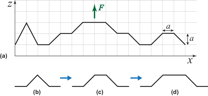
Figure 1: (a) 2D GB composed of straight segments connecting nodes of an $a\times a$ square grid. The GB can migrate under an applied force $F$ by stochastic displacements of the nodes by $\pm a$ at a time parallel to the $z$-axis. (b) Elementary excitation of a planar GB. (c) The excitation grows when a neighboring node makes a jump forward, forming a double kink. (d) Another jump causes further growth of the kink pair.

In the 2D version of the model, the GB is a 1D object (curve) separating two 2D grains. The model is illustrated in Fig. 1(a). The GB is composed of $N$ straight segments connecting the nodes of an imaginary $a\times a$ grid. The nodes are at $x_{i}=ia$, $z_{i}=ja$, where $i=0,1,...,N-1$ and $j$ are integers. The periodic boundary condition $z_{N}=z_{0}$ is imposed. The nodes can be interpreted as structural units of the GB. Each GB segment $[i,i+1]$ is assigned the excess energy

$$\varepsilon_{i}=\gamma a\left[\sqrt{a^{2}+(z_{i+1}-z_{i})^{2}}-a\right],$$ (1)

where $\gamma$ is the GB energy per unit area assumed to be the same for all segments. For a planar interface all $\varepsilon_{i}=0$.

Each GB node $i$ is acted upon by two forces: (1) external force $F$ applied parallel to the $z$-axis, and (2) local interface tension $\varepsilon_{i-1}+\varepsilon_{i}$. At a finite temperature, each node executes a driven random walk along the $z$-axis.

The model falls in the category of solid-on-solid (SOS) models (Swendsen:1977, ; Lapujoulade:1994uw, ; Hasenbusch:1996wn, ; LandauBinder09, ), which were originally developed for surface roughening and crystal growth from a vapor phase. SOS models have several versions, depending on the algorithm for computing the excess energy. The best-known of them are the discrete Gaussian SOS (DGSOS) model with

$$\varepsilon_{i}=\gamma(z_{i+1}-z_{i})^{2},$$ (2)

and the absolute SOS (ASOS) model with

$$\varepsilon_{i}=\gamma a\left|z_{i+1}-z_{i}\right|.$$ (3)

A 3D DGSOS model was recently used to simulate solute drag by moving GBs (Wicaksono:2013aa, ). There is no compelling physical reason to prefer one SOS version over another. The ansatz in Eq.(1) interpolates between the DGSOS and ASOS versions. It converges to the ASOS version when $\left|z_{i+1}-z_{i}\right|\gg a$ but regularizes the discontinuity of the energy derivative with respect to the inclination angle at $z_{i}=z_{i+1}$.

To describe the GB dynamics, we adopt the harmonic transition state theory (TST) (Vineyard:1957vo, ), by which the forward ($+$) and backward ($-$) transition (jump) rates of any GB node $i$ are $\omega_{i}^{\pm}=\nu_{0}P_{i}^{\pm}$, where $\nu_{0}$ is the attempt frequency assumed to be constant,

$$P_{i}^{\pm}=\exp\left(-\dfrac{E_{i}^{\pm}}{k_{B}T}\right)$$ (4)

are the jump probabilities, and $k_{B}$ is Boltzmann’s constant. The jump barriers $E_{i}^{\pm}$ are given by

$$E_{i}^{\pm}=\begin{cases}E_{ti}\exp\left(\dfrac{u_{i}^{\pm}}{2E_{ti}}\right),&u_{i}^{\pm}\leq 0,\\ u_{i}^{\pm}+E_{ti}\exp\left(-\dfrac{u_{i}^{\pm}}{2E_{ti}}\right),&u_{i}^{\pm}>0,\end{cases}$$ (5)

where $u_{i}^{\pm}$ is the total energy change due to the jump. This energy change includes the work $\mp Fa$ against the external force $F$ and the energy changes, $\Delta\varepsilon_{i-1}$ and $\Delta\varepsilon_{i}$, of the two GB segments connected to node $i$:

$$u_{i}^{\pm}=\mp Fa+\Delta\varepsilon_{i-1}+\Delta\varepsilon_{i}.$$ (6)

As discussed in Part I (Mishin_2023_RW_part_I, ), the exponential terms in Eq.(5) ensure that the barriers decrease with increasing force $-u_{i}^{\pm}/a$ but never become strictly zero. Previous models (Cahn:2001wh, ; Cottrell:2002ub, ; Ivanov08a, ; Chachamovitz:2018vm, ) assumed that a barrier could be suppressed to zero at a critical value of the force. In the present model, the zero-barrier point is regularized by replacing it with an exponential decay as the force increases.

The variable $E_{ti}$ in Eq.(5) is the unbiased (when $u_{i}^{\pm}=0$) jump barrier. In the absence of pinning, the unbiased barrier is $E_{0}$, which is a model parameter. The unpinned and unbiased residence time of any GB node is

$$t_{0}=\dfrac{1}{2\nu_{0}}\exp\left(\dfrac{E_{0}}{k_{B}T}\right).$$ (7)

The pinning raises the unbiased jump barrier to $E_{ti}>E_{0}$. Accordingly, the biased jump barriers $E_{i}^{\pm}$ given by Eq.(5) also increase. In the KMC simulations, the increase of the barriers due to the pinning effect is implemented by the following algorithm. After arriving at the current state $i$, the GB node attempts to make a new jump. After each unsuccessful attempt, we penalize the node by increasing the jump barriers for both escape routes from the state $i$. After $n$ unsuccessful attempts, the unbiased barrier becomes

$$E_{ti}=E_{0}\left(1+(\alpha-1)\dfrac{\sqrt{t/t_{p}}}{1+\sqrt{t/t_{p}}}\right),$$ (8)

where $t=n/2\nu_{0}$ is the discrete time variable. Here, $\alpha>1$ is the pinning strength coefficient and $t_{p}>0$ is the pinning time, both model parameters. After the node finally makes a successful jump, the attempt counter $n$ is reset to zero and the process repeats from the new state. When $t\ll t_{p}$, the barriers grow with time as $\sqrt{t}$. The square root time dependence reflects the diffusion kinetics of the solute supply to the GB, causing its pinning. If a successful jump takes a long time $t\gg t_{p}$, the barrier plateaus at $E_{ti}=\alpha E_{0}\equiv E_{\infty}>E_{0}$. This long-time limit represents the saturation of the segregation atmosphere. Once the atmosphere is saturated, the GB displacements are controlled by the fully pinned barrier $E_{\infty}$. The most interesting and complex is the intermediate kinetic regime in which $t_{p}$ is close to the escape time $t_{0}$. We refer to this kinetic regime as active pinning.

The process described above was implemented in KMC simulations. At each KMC step, three random numbers $(r_{1},r_{2},r_{3})$ are drawn uniformly from a unit interval. The first number $r_{1}$ chooses a GB node, say $i$, for an attempt. All nodes can be chosen with equal probability. Then $r_{2}$ chooses between a forward jump or a backward jump, also with equal probability. Finally, $r_{3}$ decides if the attempt is successful according to the jump probability $P_{i}^{\pm}$. If the attempt fails, the counter of unsuccessful attempts at site $i$ is advanced by $1$ and $E_{ti}$ is raised according to Eq.(8). If the jump is successful, the node $i$ is shifted by $\pm a$ along the $z-$axis, the counter of failed attempts is reset to 0, and the jump probabilities at nodes $i-2,$ $i-1$, $i$, $i+1$, and $i+2$ are updated. After $2N$ KMC attempts, the clock is advanced by $\nu_{0}^{-1}$. Other details of the KMC algorithm were discussed in Part I (Mishin_2023_RW_part_I, ).

III Equilibrium grain boundary properties

We will first investigate GB properties in the absence of external forces ($F=0$). The GB is then only subject to equilibrium thermal fluctuations. Analysis of this case will create a baseline for comparison with moving GBs discussed later in section IV. In addition, since the present SOS model is distinct from previous versions, a detailed characterization of equilibrium GB properties will inform future applications of the model

III.1 Theoretical background

Without external forces, the average GB position

$$z_{*}=\dfrac{1}{N}\sum_{i=0}^{N-1}z_{i}$$ (9)

executes an unbiased random walk while the GB shape fluctuates due to energy exchanges with the thermostat. The GB properties can be characterized by the following quantities:

• Excess GB energy

  $$\overline{\varepsilon}\equiv\dfrac{1}{N}\overline{\left(\sum_{i=0}^{N-1}\varepsilon_{i}\right)}$$ (10)

  and the mean squared excess GB energy

  $$\overline{\varepsilon^{2}}\equiv\dfrac{1}{N}\overline{\left(\sum_{i=0}^{N-1}\varepsilon_{i}^{2}\right)},$$ (11)

  where the bar indicates averaging over a long time.

• GB heat capacity per node computed from the energy fluctuation formula

  $$C=N\dfrac{\overline{\varepsilon^{2}}-\overline{\varepsilon}^{2}}{k_{B}T^{2}}.$$ (12)

  Note that the GB heat capacity can also be calculated directly by $C=d\overline{\varepsilon}/dT$.

• Excess GB area $\bar{s}\equiv\bar{\varepsilon}/\gamma$.

• Mean squared GB width

  $$\overline{w^{2}}\equiv\dfrac{1}{N}\overline{\left(\sum_{i=0}^{N-1}w_{i}^{2}\right)},$$ (13)

  where

  $$w_{i}\equiv z_{i}-z_{*}.$$ (14)

• The GB “flatness” parameter $f$ defined as the fraction of parallel segments ($z_{i}=z_{i+1}$) relative to the total number of segments.

• Energy self-correlation function

  $$K(t)=\dfrac{\left\langle\varepsilon(t)\varepsilon(0)\right\rangle-\overline{\varepsilon}^{2}}{\overline{\varepsilon^{2}}-\overline{\varepsilon}^{2}},$$ (15)

  where $\varepsilon(t)$ is the instantaneous interface excess energy per node and the angular brackets indicate averaging over initial states ($t=0$) along a long simulation trajectory.

The GB structure is expected to be nearly planar with a small number of thermal kinks when $k_{B}T\ll\gamma a^{2}$ and rugged and wavy when $k_{B}T\gg\gamma a^{2}$. A transition from the first structure, called “smooth”, to the second one, called “rough”, can be expected to occur when $\gamma a^{2}$ is comparable to $k_{B}T$.

A smooth GB contains kinks as thermal excitations of the perfectly planar structure. In the present model, the lowest-energy excitation is the triangular bump shown in Fig. 1(b). Its excess energy is

$$u_{2k}=2u_{k}=2(\sqrt{2}-1)\gamma a^{2}$$ (16)

and the formation barrier in the absence of pinning is

$$E_{2k}=u_{2k}+E_{0}\exp\left(-\dfrac{u_{k}}{E_{0}}\right),$$ (17)

where $u_{k}=(\sqrt{2}-1)\gamma a^{2}$ is the single-kink energy. One of the base nodes of the triangular bump can jump forward to form a double kink (Fig. 1(c)). The barrier of this jump is $E_{0}<E_{2k}$ and the GB energy does not change. The next jump, shown in Fig. 1(d), causes further separation of the kinks; it has the same barrier $E_{0}$ and does not change the GB energy either. Thus, the triangular bump is the critical nucleus of the kink pair formation. Since the kink pair nucleation barrier $E_{2k}$ is higher than the kink migration barrier $E_{0}$, the kink pair formation at a smooth GB is a nucleation-controlled process.

The thermal kink concentration (probability per node) on a smooth GB is (Hirth, ; Saito:1996vo, )

$$n_{k}=2\exp\left(-\dfrac{u_{k}}{k_{B}T}\right),$$ (18)

from which the excess GB energy is

$$\overline{\varepsilon}=2u_{k}\exp\left(-\dfrac{u_{k}}{k_{B}T}\right).$$ (19)

The GB heat capacity calculated from this energy,

$$C=\dfrac{d\overline{\varepsilon}}{dT}=\dfrac{2u_{k}^{2}}{k_{B}T^{2}}\exp\left(-\dfrac{u_{k}}{k_{B}T}\right),$$ (20)

reaches a maximum at $k_{B}T/\gamma a^{2}=(\sqrt{2}-1)/2\approx 0.21$. This maximum can be associated with the GB roughening transition. Note that the kink concentration corresponding to this maximum is $n_{k}=2e^{-2}\approx 0.27$, which is no longer small.

Above the roughening transition, the GB develops significant shape fluctuations and can be better described by the capillary wave theory (Gelfand:1990vz, ; Lapujoulade:1994uw, ; Saito:1996vo, ). For 2D interfaces, the capillary wave amplitude diverges to infinity with increasing lateral size $L=Na$. The relevant results of the theory are summarized in Appendix A. The theory predicts the mean squared GB width

$$\overline{w^{2}}=\dfrac{k_{B}TL}{12\Lambda a},$$ (21)

where

$$\Lambda=f_{0}+(\partial^{2}f/\partial\beta^{2})_{0}$$ (22)

is the GB stiffness, $f$ is the GB free energy per unit area, and $\beta$ is the small angle between the local GB orientation and the $x$-axis. The first term in the right-hand side of Eq.(22) is the GB free energy in the $\beta\rightarrow 0$ limit (perfectly planar GB). The second (“torque”) term is the second angular derivative of $f$ taken in the $\beta\rightarrow 0$ limit. It should be emphasized that the underlying assumption of the theory is that $\beta\ll 1$, i.e., $\sqrt{\overline{w^{2}}}\ll L$.

III.2 Simulation results

The KMC simulations were performed in normalized variables obtained by dividing the time, the coordinates, and all energies by $\nu_{0}^{-1}$, $a$, and $E_{0}$, respectively. The normalized temperature, force, and GB energy become, respectively,

$$\theta=\dfrac{k_{B}T}{E_{0}},\enskip\varphi=\dfrac{Fa}{E_{0}},\enskip\sigma=\dfrac{\gamma a^{2}}{E_{0}}.$$

Other normalized variables used in the simulations are summarized in Table 1. The results presented in this subsection were obtained at $\sigma=1$.

III.2.1 GB properties in the absence of pinning

We first consider the simulation results in the absence of pinning. Recall that the GB is not acted upon by any external force ($\varphi=0$).

Figure 2 shows typical structures of a smooth GB with a small concentration of kinks, a rough GB with capillary waves, and a moderately rough GB in between. As expected, the GB evolves from smooth to rough with increasing temperature.

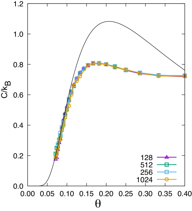
Figure 3: GB heat capacity as a function of temperature $\theta$ at $\sigma=1$ for several system sizes $N$ indicated in the key. The boundary is not subject to external forces or solute pinning. As $N$ increases by nearly an order of magnitude, the heat capacity curves coincide within the statistical scatter. The solid curve is predicted by Eq.(20) based on the kink model.

To understand the nature of the roughening transition, we examine the temperature dependence of the GB heat capacity computed from the fluctuation formula (12). Figure 3 shows that the heat capacity obtained by the simulations reaches a maximum when $\theta/\sigma$ is reasonably close to 0.2, as predicted by the kink model mentioned above. The simulations accurately follow Eq.(20) at low temperatures when the GB is fairly smooth. The agreement worsens with temperature, and the maximum predicted by Eq.(20) significantly overshoots the simulation results. This is unsurprising given that the GB structure near the maximum is intermediate between smooth and rough, and the kink model is a crude approximation. For a true phase transformation, the height of the heat capacity maximum must increase with the system size and diverge to infinity in the thermodynamic limit ($N\rightarrow\infty$). By contrast, the heat capacity obtained by the simulations is virtually independent of the system size. Thus, in the present model, the GB roughening is a continuous transformation. Continuous roughening was also predicted by other models of 2D interfaces (Lapujoulade:1994uw, ; LandauBinder09, ; Saito:1996vo, ).

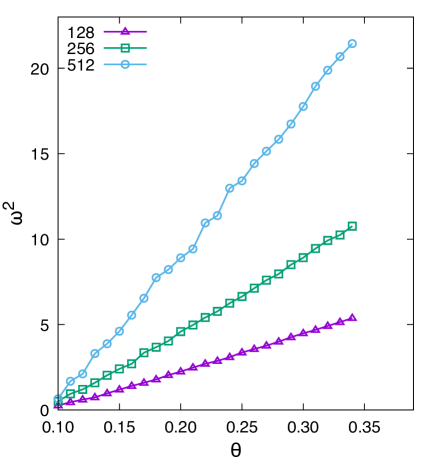
(b)

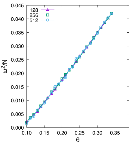
Figure 4: (a) Mean squared GB width $\overline{\omega^{2}}$ as a function of temperature $\theta$ at $\sigma=1$ for three system sizes $N$ indicated in the key. The monotonic increase of $\overline{\omega^{2}}$ with $N$ proves the GB roughness. (b) The plots of $\overline{\omega^{2}}/N$ versus $\theta$ for different $N$ values collapse into a single curve, confirming the size scaling predicted by Eq.(21).

In the capillary wave regime, Eq.(21) predicts that the mean squared GB width $\overline{\omega^{2}}$ increases with the system size $N$ and diverges to infinity at $N\rightarrow\infty$. This divergence is considered a formal definition of a rough interface. The expected increase of $\overline{\omega^{2}}$ with $N$ is indeed observed in the simulations (Fig. 4(a)), confirming that the GB is officially rough above $\theta\approx 0.2$. Furthermore, the plots of $\overline{\omega^{2}}/N$ versus $\theta$ for different $N$ values collapse into a single master curve (Fig. 4(b)) as predicted by Eq.(21). This curve allows us to extract the normalized interface stiffness $\lambda$ using the dimensionless form of Eq.(21):

$$\lambda=\dfrac{\theta}{12\left(\overline{\omega^{2}}/N\right)}.$$ (23)

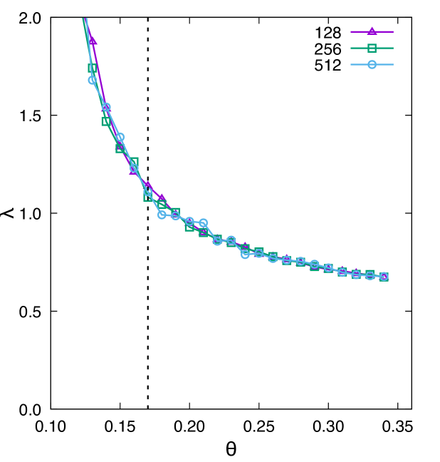
Figure 5: GB stiffness $\lambda$ as a function of temperature computed from Eq.(23) at $\sigma=1$ for three different system sizes $N$. The dashed line marks the approximate location of the GB roughening transition.

The stiffness obtained from this equation is plotted as a function of temperature in Fig. 5. The sharp increase in $\lambda$ below the roughening transition is an artifact because the capillary wave model is only valid for rough interfaces. The fact that $\lambda$ decreases with increasing temperature points to a significant contribution of the configurational entropy to the GB free energy associated with the GB shape fluctuations.

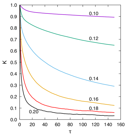
(b)

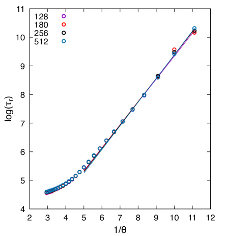
Figure 6: (a) Energy self-correlation function $K(\tau)$ for $N=256$ and $\sigma=1$ at several temperatures $\theta$ indicated in the labels. (b) Arrhenius diagram of the energy relaxation time $\tau_{r}$ for different system sizes indicated in the key. The straight lines are linear fits to the low-temperature portions of the curves.

Figure 6(a) illustrates typical energy self-correlation functions $K(\tau)$ at several temperatures including both smooth and rough GB structures. The correlation decay rate increases with temperature, as it should for a thermally activated process. The decay rate can be quantified by extracting the relaxation time $\tau_{r}$ by fitting the short-time portion of $K(\tau)$ with the exponential relation $K=K_{0}\exp(-\tau/\tau_{r})$, where $K_{0}$ is a constant. The relaxation times obtained are plotted in the Arrhenius coordinates $\ln\tau_{r}$ versus $1/\theta$ in Fig. 6(b). Observe that the curves corresponding to different system sizes coincide within the scatter of the points, confirming the local nature of the short-time relaxation. The Arrhenius plots are fairly linear at low temperatures but develop a significant upward deviation above the roughening transition. The low-temperature portions of the curves, corresponding to smooth GB structures, were fitted with the Arrhenius relation

$$\tau_{r}=\tau_{r}^{0}\exp\left(-\dfrac{\varepsilon_{a}}{\theta}\right),$$ (24)

where $\tau_{r}^{0}$ is a constant. The activation energies $\varepsilon_{a}$ extracted from the fits were found to be practically the same for all system sizes and equal to $\varepsilon_{a}=0.821$. This number is reasonably close to the normalized kink pair energy $u_{2k}/E_{0}=2(\sqrt{2}-1)\sigma=0.828$, see Eq.(16) above and recall that $\sigma=1$ in the simulations. This agreement confirms that the dominant relaxation mechanism in a smooth GB is the nucleation and recombination of thermal kink pairs. The non-Arrhenius deviation at high temperatures reflects the gradual transition from the smooth to the rough GB structure when the fluctuations form capillary waves. Under such conditions, the relaxation mechanism involves collective rearrangements of the high concentration of geometrically necessary kinks accommodating the GB curvature. Such rearrangements occur on a greater length scale than in a smooth GB, causing the significant increase in the relaxation time.

III.2.2 GB properties with pinning

The effect of pinning on the equilibrium GB properties is controlled by the relative pinning time $\tau_{p}/\tau_{0}$, where $\tau_{0}=t_{0}\nu_{0}$ is the unpinned residence time. To investigate the pinning effect, the KMC simulations were performed at several fixed values of $\tau_{p}/\tau_{0}$ spanning the range from 0.01 to 100. As temperature was increased, $\tau_{0}$ decreased (cf. Eq.(7)) but $\tau_{p}$ was adjusted to keep $\tau_{p}/\tau_{0}$ constant. The GB energy and the pinning strength were fixed at $\sigma=1$ and $\alpha=1.5$, respectively.

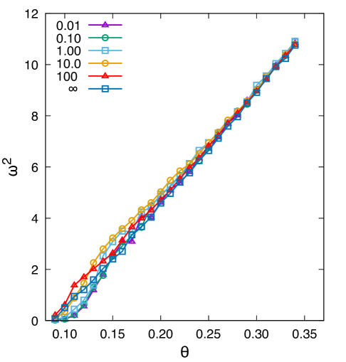
(b)

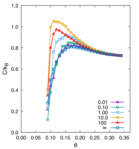
Figure 7: Effect of pinning on GB properties without driving forces. The KMC simulations were performed at $N=256$, $\sigma=1$, and several values of the relative pinning time $\tau_{p}/\tau_{0}$ indicated in the key. The curve labeled $\infty$ corresponds to the absence of pinning. (a) Mean squared GB width $\overline{\omega^{2}}$ as a function of temperature $\theta$. (b) GB heat capacity as a function of temperature $\theta$.

The general trend observed in the simulations is that the active pinning promotes GB roughness. For example, Figure 7(a) presents the mean squared GB width $\overline{\omega^{2}}$ plotted as a function of temperature for a set of $\tau_{p}/\tau_{0}$ values. At temperatures well above the roughening transition, $\overline{\omega^{2}}$ is practically independent of $\tau_{p}/\tau_{0}$ and increases as a linear function of temperature, as predicted by the capillary-wave equation (21). Thus, the pinning has little effect on the rough GB structure. As temperature decreases and the GB becomes smoother, $\overline{\omega^{2}}$ deviates from the linear behavior. At large and small $\tau_{p}/\tau_{0}$ values, $\overline{\omega^{2}}$ approaches the simulation results obtained in the absence of pinning (the curve labeled $\infty$). At intermediate $\tau_{p}/\tau_{0}$ values corresponding to the active pinning regime (e.g., $\tau_{p}/\tau_{0}$ between 1 and 10), $\overline{\omega^{2}}$ displays upward deviations that grow as temperature decreases. The GB becomes wider and thus rougher compared with the unpinned and fully pinned cases. At even low temperatures, $\overline{\omega^{2}}$ converges to zero as the GB attains a smooth structure. In other words, the pinning effect on the GB width is strongest at temperatures near the roughening transition and when the pinning time $\tau_{p}$ is on the order of $\tau_{0}$.

These observations are consistent with the temperature dependence of the heat capacity shown Figure 7(b). It should be reminded that the fluctuation formula (12) does not necessarily give the correct heat capacity under the active pinning conditions because the KMC simulations become non-Markovian (Mishin_2023_RW_part_I, ). Nevertheless, the heat capacity obtained from Eq.(12) can be used as simply a measure of energy fluctuations, which are expected to grow near the roughening transition. As with the mean squared GB width, at temperatures above the roughening transition, the heat capacity is unaffected by pinning: the results obtained at all $\tau_{p}/\tau_{0}$ values converge to the same curve obtained by unpinned simulations. At large and small $\tau_{p}/\tau_{0}$ values, the heat capacity continues to follow the unpinned curve. However, in the active pinning regime, the heat capacity displays significant upward deviations at temperatures close to the roughening transition. Taking the peak position as the transition temperature, we observe that active pinning shifts the roughening transition temperature down and makes the transition sharper.

IV Grain boundary dynamics

IV.1 GB dynamics in the absence of pinning

Now suppose that the GB is acted upon by an external force $F$. We first disregard the pinning effect and consider the motion of a chemically pure GB.

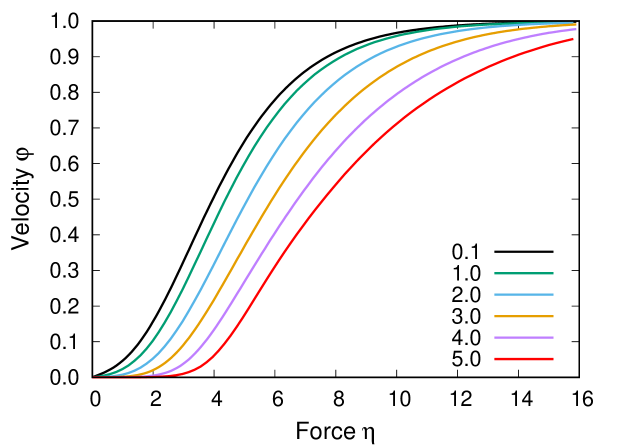
Figure 8: Velocity-force relations in the 2D GB model with $N=512$ nodes at the temperature of $\theta=0.2$ for several values of the GB energy $\sigma$ indicated in the key. The GB is not subject to pinning.

Examples of velocity-force functions obtained by the simulations are shown in Fig. 8 for several values of the normalized GB energy $\sigma$. The simulation temperature is fixed at $\theta=0.2$, which is close to the roughening transition in a stationary GB. Since large GB energy enforces planar GB shape, one would expect that, as $\sigma$ increases, the velocity-force curves should approach those predicted by the 1D model. Contrary to this expectation, it is the lowest-energy curve ($\sigma=0.1$) that is practically indistinguishable from the curve computed previously (Mishin_2023_RW_part_I, ) within the 1D model (not shown in the figure). As $\sigma$ increases, the 2D results increasingly deviate from the 1D model. The curves develop a nearly flat portion at low velocities, followed by a rapid rise as the driving force increases. Similar shapes of velocity-force functions were seen in some of the previous 2D and 3D simulations of interface dynamics (Mendelev02a, ; Mendelev:2001aa, ; Mendelev:2001wk, ; Mendelev:2002wv, ; Wicaksono:2013aa, ). Note that a stationary GB with $\sigma=0.1$ is rough, a stationary GB with $\sigma=1$ is transitional between rough and smooth, and stationary GBs with $\sigma=2$, $3$, $4$ and $5$ are smooth. Two conclusions can be drawn from these observations:

• 1D models, including the classical models (Cahn-1962, ; Lucke-Stuwe-1963, ; Lucke:1971aa, ), should be interpreted as representing driven motion of the average plane of a rough GB.

• Smooth GBs strongly deviate from the classical models by displaying much lower mobility.

The mechanism of the latter deviation is as follows. Smooth GBs undergo a dynamic roughening transition as the velocity increases at a fixed temperature. This transition alters the migration mechanism and increases the GB mobility. The migration mechanism is mediated by the motion of kink pairs when the GB is smooth and by a biased random walk of the average GB plane when the GB becomes rough. As mentioned above, a rough GB contains a high concentration of geometrically necessary kinks accommodating the capillary waves. Their motion is responsible for both the capillary fluctuations and, in the presence of a driving force, for the drift of the average GB plane. Due to the large kink concentration, the GB mobility is high. By contrast, a smooth GB contains a small concentration of thermal kinks that can only support slow GB migration. A large enough force can cause the nucleation of additional (non-equilibrium) kinks and eventually cause a dynamic roughening transition. The latter, in turn, accelerates the GB migration and is responsible for the sigma shape of the velocity-force curves at large $\sigma$ values (Fig. 8).

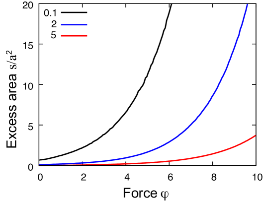
Figure 9: Excess GB area $s$ (normalized by $a^{2}$) as a function of driving force at the temperature of $\theta=0.2$ for three values of the GB energy $\sigma$. At each value of the force, $s$ was obtained by averaging over a long time in the steady-state regime. The system size is $N=512$ and the GB is not subject to pinning.

The dynamic roughening transition is illustrated Figure 9 using the excess area $s$ as a measure of GB roughness. In the stationary state ($F=0$), the three GBs shown in this plot are, respectively, smooth ($\sigma=5$), intermediate ($\sigma=1$), and rough ($\sigma=0.1$). When a force is applied and causes GB motion, the GB roughness increases with the force. The initially smooth GB develops non-equilibrium kinks and eventually reaches the excess area characteristic of rough GBs. The initially rough interface becomes even rougher. Fig. 10 visually represents the dynamic roughening transition with increasing velocity. As in the stationary case, this transition is continuous.

We next discuss the kink-mediated migration of a smooth GB in more detail. Several models of interface migration by the kink pair mechanism were proposed (Hirth, ; Bertocci-1969, ; Seeger-1981, ; Mendelev:2001wk, ). (We note in passing that the problem is similar to kink-mediated dislocation glide if elastic effects are neglected.) We assume that the kinks only nucleate by pairs and their thermally equilibrium concentration is small. The driving force reduces the barrier of forward GB jumps and creates a relatively high concentration $n_{2k}$ of non-equilibrium kink pairs (number per unit area) bounding GB segments displaced in the force direction. The force also biases the barriers of kink jumps parallel to the GB plane, driving kink separation in each pair. The kink pair growth velocity is $2v$, where $v$ is the single-kink drift velocity along the planar boundary given by

$$v=a\nu_{0}\left[\exp\left(-\dfrac{E^{(+)}}{k_{B}T}\right)-\exp\left(-\dfrac{E^{(-)}}{k_{B}T}\right)\right],$$ (25)

where

$$E^{(+)}=E_{0}\exp\left(-\dfrac{Fa}{2E_{0}}\right)$$ (26)

is the forward jumps barrier and

$$E^{(-)}=Fa+E_{0}\exp\left(-\dfrac{Fa}{2E_{0}}\right)$$ (27)

is the backward jump barrier. The velocity-force relation predicted by Eq.(25) is linear under a small force and becomes nonlinear as the force increases.

Suppose the GB is initially planar and the applied force causes the nucleation of $J$ kink pairs per unit area per unit time. After a time $t$, the pair concentration becomes $n_{2k}=Jt$. During this time, the nuclei grow to the average size $2vt$. The time required to form a contiguous new layer is found from the condition $2vt=l_{2k}$, where $l_{2k}=1/n_{2k}a$ is the average distance between the nucleation centers. This crude estimate gives the time $t=1/\sqrt{2avJ}$ in which the GB displaces a distance $a$ (one layer thickness) in the force direction. For the GB velocity $v_{2k}=a/t$ we then have

$$v_{2k}=a\sqrt{2avJ,}$$ (28)

where the subscript $2k$ indicates that this velocity is specific to the kink pair mechanism. Equation (28) was previously derived by Bertocci (Bertocci-1969, ) by a different method.

The next step is to calculate the nucleation rate $J$. This rate is controlled by the nucleation rate of triangular bumps shown in Fig. 1(b):

$$J=\dfrac{\nu_{0}}{a^{2}}P_{01}P_{s},$$ (29)

where

$$P_{01}=\exp\left(-\dfrac{u_{2k}-Fa+E_{0}e^{-(u_{2k}-Fa)/2E_{0}}}{k_{B}T}\right)$$ (30)

is the probability per one attempt that a given node on a planar GB (call it state 0) pops up to form a triangular bump (call it state 1). The factor $P_{s}$ in Eq.(29) is the probability of survival of the bump. Indeed, the bump can disappear by a reverse jump $1\rightarrow 0$ whose probability per attempt is

$$P_{10}=\exp\left(-\dfrac{E_{0}e^{-(u_{2k}-Fa)/2E_{0}}}{k_{B}T}\right).$$ (31)

Alternatively, the triangular bump can expand into a kink pair containing two GB nodes (state 2) as shown in Fig. 1(c). This kink pair can collapse back into the triangular bump (jump $2\rightarrow 1$) or expand further. The kink separation will then execute a driven random walk in which it will most likely keep expanding indefinitely. But there is a chance that the kink pair eventually collapses back into a triangular bump. $P_{s}$ is the probability that such a collapse does not happen. As shown in Appendix B,

$$P_{s}=\dfrac{2(P_{12}-P_{21})}{P_{10}+2(P_{12}-P_{21})}.$$ (32)

Here,

$$P_{12}=\exp\left(-\dfrac{E_{0}e^{-Fa/2E_{0}}}{k_{B}T}\right)$$ (33)

and

$$P_{21}=\exp\left(-\dfrac{Fa+E_{0}e^{-Fa/2E_{0}}}{k_{B}T}\right)$$ (34)

are the $1\rightarrow 2$ and $2\rightarrow 1$ jump probabilities (per attempt), respectively. Note that they are related to the single-kink drift velocity (25) by

$$v=a\nu_{0}(P_{12}-P_{21}).$$ (35)

Putting all pieces together, the GB velocity by the kink pair mechanism becomes

$$v_{2k}=2v\left(\dfrac{P_{01}}{P_{10}+2(P_{12}-P_{21})}\right)^{1/2}.$$ (36)

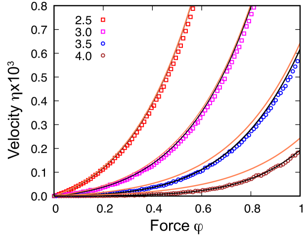
Figure 11: Zoom into the low-velocity portions of the velocity-force curves shown in Fig. 8. The GB energies $\sigma$ are indicated in the key. The points represent KMC simulation runs. The orange curves are predicted by Eq.(36) based on the kink pair GB migration model neglecting the system size effect. The black curves are predicted by Eq.(39) including the system size correction.

Figure 11 shows that Eq.(36) compares with the KMC simulations reasonably well when the GB energy is not too high. However, it increasingly overestimates the velocity as the GB energy increases. This is understandable because the nucleation rate decreases with increasing GB energy, and the nuclei spacing $l_{2k}$ eventually reaches the system size $L=Na$ ($N=512$ in the simulations). The GB migration becomes strongly nucleation-controlled. A single nucleation event triggers rapid expansion of the kink pair to the system size before another pair has a chance to nucleate. The expectation time of the nucleation event is $t=(JaL)^{-1}$. Thus, instead of Eq.(28), the GB velocity becomes

$$v_{2k}=a/t=Ja^{2}L.$$ (37)

Note that Eq.(28) can be written in the form $v_{2k}=Ja^{2}l_{2k}$, showing that the nucleation-controlled case is obtained by replacing $l_{2k}$ with $L.$

It was proposed (Hirth, ; Seeger-1981, ) to capture the system size dependence by multiplying $v_{2k}$ by the interpolating function $L/(L+l_{2k})$ with $l_{2k}$ calculated for an infinitely large system. It is easy to show that

$$l_{2k}=\left(\dfrac{2v}{aJ}\right)^{1/2}=a\left(\dfrac{P_{10}+2(P_{12}-P_{21})}{P_{01}}\right)^{1/2}.$$ (38)

Comparison with the KMC simulations shows that this interpolating function overcorrects the model by under-predicting the GB velocity (not shown in Fig. 8). Note that the choice of the interpolating function is arbitrary as long as it gives the correct values of 1 and $L/l_{2k}$ in the limits of $l_{2k}\ll L$ (infinitely large system) and $l_{2k}\gg L$ (small system), respectively. For example, we find that the function $L/(L^{2}+l_{2k}^{2})^{1/2}$ provides much better agreement with the simulations of high GB energies (Fig. 11). The respective GB velocity is

$$v_{2k}=2v\left(\dfrac{P_{01}}{\left[P_{10}+2(P_{12}-P_{21})\right]\left(1+l_{2k}^{2}/L^{2}\right)}\right)^{1/2}$$ (39)

with $l_{2k}$ given by Eq.(38).

The demonstrated agreement between the kink pair model and the simulation results corroborates our explanation that the peculiar S-shape of the velocity-force relations in Fig. 8 is caused by a transition of the GB migration mechanism from (1) kink pair nucleation and growth under a small force to (2) driven random walk of a rough GB structure under a larger force.

IV.2 GB dynamics with pinning

We now consider a GB subject to the pinning effect. It is convenient to discuss the impact of pinning in terms of the normalized solute diffusivity $D/D_{0}$ rather than the normalized pinning time $\tau_{p}/\tau_{0}$ as in section III.2.2. The relation between the two is $D/D_{0}=\tau_{0}/\tau_{p}$ (Mishin_2023_RW_part_I, ). In the simulations presented below, $D/D_{0}$ was varied while the pinning strength was fixed at $\alpha=1.5$.

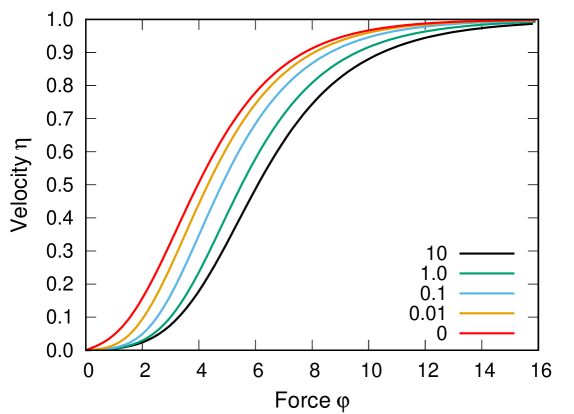
(b)

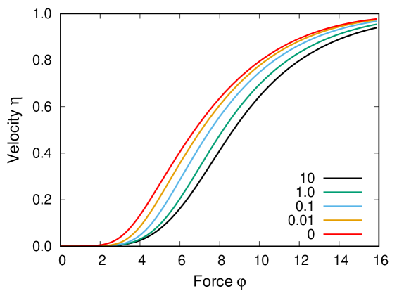
Figure 12: Velocity-force relations for the 2D GB with $N=512$ nodes at the temperature of $\theta=0.2$ for several values of the normalized solute diffusivity $D/D_{0}$ indicated in the key. The curve for $D/D_{0}=0$ was obtained by simulations without pinning. (a) $\sigma=0.1$; (b) $\sigma=4.0$.

As expected, we find that the pinning always reduces the GB velocity under a given driving force relative to the unpinned case (Fig. 12), which is a manifestation of the solute drag effect. As also expected, faster solute diffusion (larger $D/D_{0}$) causes stronger retardation of the GB motion. This is understandable because a faster solute can keep up with the moving GB and slow it down. The S-shape of the velocity-force curves becomes more pronounced, especially for high-energy GBs (Fig. 12(b)). As discussed in the previous subsection, the S-shape is caused by the dynamic roughening effect. Since the pinning reduces the GB velocity, it partially suppresses the dynamic roughening. The slow kink pair migration mechanism continues to operate until larger forces, causing the nearly flat portion of the curves in the low-velocity regime.

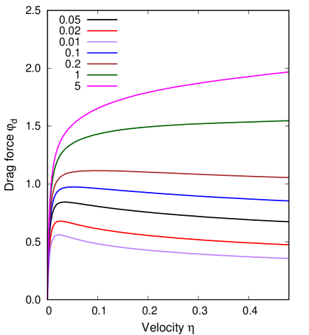
(b)

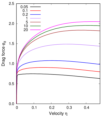
Figure 13: Solute drag force $\varphi_{d}$ as a function of velocity $\eta$ for the 2D GB with $N=512$ nodes at the temperature of $\theta=0.2$ for several values of the normalized solute diffusivity $D/D_{0}$ indicated in the key. (a) $\sigma=0.1$; (b) $\sigma=4.0$.

The solute drag force is defined as the difference between the force required to drive the GB in the presence of pinning and the force to drive an unpinned GB with the same velocity (Mishin_2023_RW_part_I, ). In Fig. 12, the drag force is the horizontal distance between the pinned curves and the unpinned curve corresponding to $D/D_{0}=0$. The velocity dependence of the normalized drag force $\varphi_{d}$ is shown in Fig. 13 for several values of $D/D_{0}$. For the low-energy GB ($\sigma=0.1$), the drag-velocity curves look qualitatively similar to those in the 1D model (Mishin_2023_RW_part_I, ), except that the magnitude of the drag force is systematically higher. As long as the solute diffusivity is not too high, the drag force reaches a maximum at a critical velocity, as predicted by the classical solute drag models (Cahn-1962, ; Lucke-Stuwe-1963, ; Lucke:1971aa, ) and confirmed in the 1D version of the present model (Mishin_2023_RW_part_I, ). Recall that on the left of the maximum, the GB drags the segregation atmosphere, while on the right of the maximum, it breaks away from it.

As in the 1D case (Mishin_2023_RW_part_I, ), some results of the 2D simulations deviate from predictions of the classical models. This includes Cahn’s (Cahn-1962, ) prediction that the maximum drag force is independent of the solute diffusivity. Figure 13 shows that the maximum value of $\varphi_{d}$ strongly depends on the solute diffusivity. Fast solute diffusion amplifies the drag by increasing the height of the maximum and shifting it towards larger velocities. When $D/D_{0}$ is large enough, the maximum smooths out. The breakaway regime disappears, and the drag force becomes a monotonically increasing function of GB velocity. The atmosphere remains permanently attached to the GB and evolves continuously from heavy when the GB moves slowly to light when it moves fast.

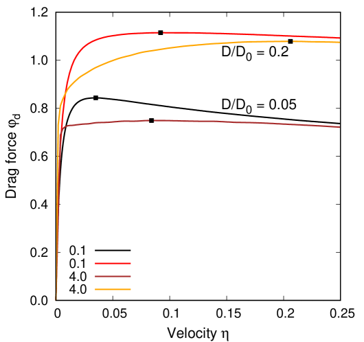
Figure 14: Solute drag force $\varphi_{d}$ as a function of velocity $\eta$ for the 2D GB with $N=512$ nodes at the temperature of $\theta=0.2$ for two values of the normalized solute diffusivity $D/D_{0}$. The GB energies $\sigma$ are indicated in the key. The points mark the maxima of $\varphi_{d}$.

An important effect revealed by the present simulations and not captured by 1D models is the impact GB roughness on the solute drag. As shown in Fig. 13, the drag-velocity curves for the high-energy GB ($\sigma=4$) have a significantly different shape than those for the low-energy boundary ($\sigma=0.1$). Recall that the former is smooth in the stationary state while the latter is rough. The difference between the two cases increases as the solute diffusivity decreases. For the high-energy GB, the low-velocity portions of curves become nearly vertical and exhibit a behavior akin to a threshold effect. Namely, the GB velocity remains extremely low until the drag force reaches a critical (threshold) level. At the critical force, the GB abruptly accelerates, producing the nearly horizontal portion on the curves. This transition is continuous but very sharp. It is further illustrated in Fig. 14, where it is especially pronounced for the high-energy GB at $D/D_{0}=0.05$. Observe that the transition occurs on the low-velocity side of the drag-force maximum where the atmosphere is attached to the GB. Note also that, on the high-velocity side of the maximum, the high- and low-energy curves converge to each other, demonstrating similar dynamics.

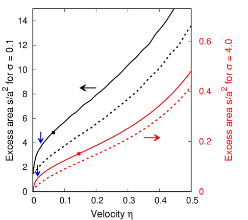
(b)

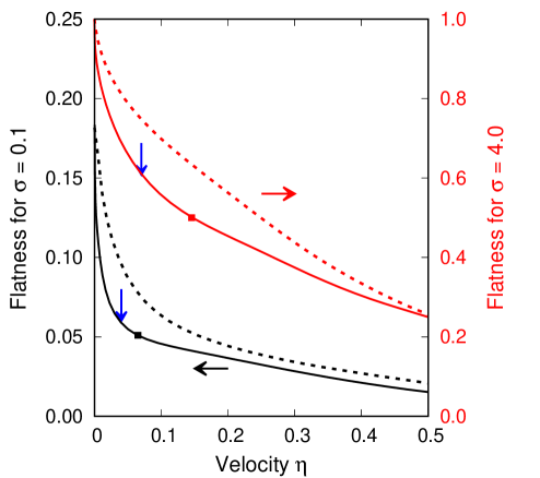
Figure 15: (a) Excess GB area $s/a^{2}$ and (b) GB flatness parameter $f$ as a function GB velocity $\eta$ for the GB energies $\sigma=0.1$ (black curves) and $\sigma=4.0$ (red curves). $s$, $f$ and $\eta$ were obtained by averaging over a long period of time after the GB motion reaches a steady state. The solid curves represent an alloy with the normalized solute diffusivity $D/D_{0}=0.1$. The dashed curves were obtained by solute-free simulations. The points mark the velocities at which the solute drag force reaches a maximum. The vertical blue arrows indicate approximate locations of the dynamic roughening transition. The temperature is $\theta=0.2$ and the system size is $N=512$.

Analysis shows that the threshold behavior of the solute drag is caused by the dynamic roughening effect. The latter was previously demonstrated for unpinned GBs (see Figs. 9 and 10). It was shown that a smooth GB becomes rough when driven by an external force. This effect is reproduced in Fig. 15, where we use the excess GB area and the GB flatness parameter $f$ as measures of roughness. This time we include the simulation results obtained in the presence of pinning. The plots show that the excess area increases and the flatness decreases with the GB velocity in all cases, which is a manifestation of dynamic roughening. We also observe that pinning increases the GB roughness relative to the unpinned GB moving with the same velocity.

Furthermore, in the presence of pinning, the curves in Fig. 15 tend to develop a threshold behavior in the low-velocity limit. The nearly vertical portion of the curves indicates that the GB resists the motion. As the driving force increases, so does the GB roughness due to the reduced barriers for kink pair nucleation. The GB remains nearly pinned in place until it develops a sufficient degree of roughness. Once a high enough level of roughness is reached, the GB motion accelerates, which in turn causes further roughening. Eventually, the GB enters a kinetic regime in which its dynamic roughness increases gradually with the velocity.

Although the dynamic roughening transition is continuous, it seems reasonable to associate it with the point of maximum curvature on the roughness-velocity curves. In Fig. 15, such points are marked by vertical arrows. We emphasize that the dynamic roughening transition differs from the previously discussed static roughening transition (which is thermodynamic in nature) both conceptually and in the degree of roughness reached at the transition point. Dynamic roughening also occurs without pinning when it is more diffuse (spread over a wider interval of velocities). The pinning shifts the transition towards smaller velocities and makes it much sharper. This causes the threshold behavior of the solute drag seen in Figs. 9 and 10. Thus, the dynamic roughening transition in GBs can strongly impact the solute drag dynamics, especially for high-energy GBs that are smooth under stationary conditions.

V Discussion and conclusions

We have developed a stochastic model of solute-GB interactions aiming to better understand the solute drag phenomenon. The model is very simple and contains only a small number of parameters but still captures the main physics of solute interactions with both stationary and moving GBs. The model describes the kinetic competition between GB migration and solute diffusion, which is the key mechanism of the solute drag. The solute diffusion is included in the model indirectly through the square root time dependence of the GB jump barriers. The GB dynamics is represented more accurately than in the linear approximation commonly employed in the modeling of GB migration.

Since the model is stochastic, its numerical solution requires KMC simulations. At variance to the traditional KMC simulations, the present random walk algorithm does not implement a Markov chain. As discussed in Part I (Mishin_2023_RW_part_I, ), the transitions between the GB states are memoryless but the residence time does not follow the exponential distribution, making the random walk a semi-Markov process (Chari:1994aa, ; Maes:2009aa, ; Yu:2010aa, ). As a consequence, the steady-state occupation probabilities of the GB states do not follow the Boltzmann distribution. This does not contradict the equilibrium statistical mechanics because the GB never reaches the true equilibrium. It is not only coupled to a thermostat but also interacts with a reservoir of solute atoms in a rate-dependent manner. The impact of this interaction on the steady-state occupation probabilities is strongest when the pinning time scale $\tau_{p}$ is close to the time scale $t_{0}$ of equilibrium thermal fluctuations, a situation that we call active pinning. We expect that non-Markovian behavior is a common feature of all systems exhibiting diffusion-controlled interactions with segregating solutes.

The 2D version of the model represents the GB as a solid-on-solid (SOS) interface. This choice is not the only possible option: some of the previous simulations of GB migration utilized the Ising model (Mendelev02a, ; Mendelev:2001aa, ; Mendelev:2001wk, ; Mendelev:2002wv, ). The latter has certain advantages as well as drawbacks relative to SOS models. One advantage is that the results can be mapped more easily onto other applications of the Ising model in many areas of physics. This can help interpret the results and borrow computer algorithms and experience from other fields. Furthermore, the Ising model can represent a smooth or faceted shape of an entire 2D or 3D grain. On the other hand, the Ising model can create GB protrusions with overhands and, in some cases, isolated inclusions (“bubbles”) of one grain inside the other. Such features do not reflect the typical morphologies of moving GBs. SOS models describe the GB shape by a single-valued function $z(x,y)$ avoiding overhangs and inclusions. This description is appropriate for individual moderately curved portions of a GB, but an entire grain cannot be represented. It should also be noted that SOS models are computationally faster because the KMC attempts are only made at the interface, whereas in the Ising models the “spin flip” attempts have to be made across the entire system. The computational efficiency of SOS models provides access to larger systems and enables a broader exploration of the parameter space.

The model reproduces a roughening transition in stationary GBs as temperature increases. This is a continuous transition that can be identified with the peak of the GB heat capacity. Active pinning reduces the roughening transition temperature and makes the transition sharper. The model also predicts dynamic roughening, a process in which a smooth GB becomes rough as the migration velocity increases at a fixed temperature. This is another continuous and fully reversible transition: the GB returns to the smooth state if it comes to rest. Without pinning, the dynamic roughening transition is spread over a broad velocity range. The pinning shifts this transition towards lower velocities and makes it significantly sharper.

The mechanism of dynamic roughening has been studied in great detail. In a stationary state or when the velocity is low, GB migration occurs by the kink pair mechanism, which can only sustain slow motion. The driving force reduces the barrier for kink pair nucleation in the forward direction, boosting the population of non-equilibrium kinks and increasing the GB mobility. In section IV.1, we proposed an analytical model of this process that agrees well with the simulation results. The growing kink concentration and its spatial variations eventually cause capillary waves. The GB structure becomes rough and the GB migration mechanism changes from kink-mediated to a random walk of the average GB plane. The dynamic roughening transition is responsible for the threshold behavior in GB dynamics, in which the GB moves very slowly until the driving force reaches a critical level at which the motion sharply accelerates. This threshold effect is especially strong for high-energy GBs. The solute pinning sharpens this effect and increases the force required to “unlock” the GB mobility. Somewhat similar shapes of drag-velocity curves were observed in prior KMC simulations using different methodologies (Mendelev02a, ; Mendelev:2001aa, ; Mendelev:2001wk, ; Mendelev:2002wv, ; Wicaksono:2013aa, ).

To put our results in perspective with the literature, dynamic roughening of open surfaces is known in the field of crystal growth (Balibar:1990aa, ; Tartaglino:2000aa, ). For GBs in materials, a threshold behavior similar to the one found in this paper was observed experimentally; see examples in Figures 2 and 5 in Ref. (KANG:2016aa, ), where the GB structures below and above the threshold were characterized as faceted (smooth, atomically ordered) and rough, respectively. The impact of roughening on GB mobility was studied by molecular dynamics (MD) simulations (Olmsted07a, ). The GB mobility in Ni was found to be much higher above the roughening transition than below. In another MD study (Marian:2004aa, ), screw dislocations in body-centered cubic metals underwent a dynamic transition from kink pair mediated glide at small strain rates to jerky motion of a rough dislocation line at high strain rates. Of course, dislocations present a different case for many reasons, including the prominent role of the elastic strain field and the kink-kink interactions. Nevertheless, this transition is likely another manifestation of the dynamic roughening phenomenon discussed here.

Observing static or dynamic roughening in simulations or experiment requires a particular combination of parameters, such as the GB energy, GB mobility, and (in alloys) solute segregation and solute diffusivity. Some GBs can remain smooth all the way to the melting point, while others premelt before they could undergo a roughening transition. GB faceting is another transition that can interplay with roughening but remains beyond the scope of this paper.

Both the 1D and 2D versions of the model reveal effects that were not in the classical models (Cahn-1962, ; Lucke-Stuwe-1963, ; Lucke:1971aa, ). One of them is the increase of the maximum drag force with the solute diffusivity. Further, the classical models do not capture the GB roughening and its impact on the GB migration mechanisms. Another difference is related to the breakaway branch of the drag-velocity relation. Cahn (Cahn-1962, ) considered this branch unstable with respect to velocity variations. He reasoned that, if the GB momentarily moves faster, it will lose some of the segregation atmosphere, which will allow it to move even faster. Recall that Cahn’s model treats the GB as a rigid plane. In the 2D version of our model, velocity fluctuations do occur locally, but they are suppressed by the interface tension and do not develop into a morphological instability. GB motion in the breakaway regime remains perfectly stable. The GB shape fluctuations indeed grow with the GB velocity, as seen on the roughness-velocity plots (Fig. 15). However, this increase is gradual and occurs at about the same rate as without pinning.

It should be recognized that the discreteness of the GB displacements imposed by the underlying $a\times a$ grid is a critical ingredient of the model capturing the existence of the GB structural units. It is due to this discreteness that the GB can be smooth or rough and can migrate by the kink pair mechanism. Details of the kink structure and energy may depend on the grid structure and symmetry. However, without the grid, there would be no kinks and no roughening transition.

Being very simple, the proposed model is not intended for accurate quantitative predictions for a particular material. Nevertheless, the numerical values of the parameters chosen for this work are quite realistic. For example, it was found above that the roughening transition temperature $T_{r}$ satisfies the condition $\theta_{r}/\sigma=k_{B}T_{r}/\gamma a^{2}\approx 0.2$. Taking Cu as an example, we can estimate $a\approx 0.3$ nm (between the first and second neighbors). GB energies in Cu vary widely from $\sim 0.2$ J m^-2 for low-angle GBs to $\sim 1$ J m^-2 for some of the high-angle, high-energy GBs (Cahn06b, ; Frolov2012b, ; Frolov2013, ; Hickman:2016aa, ; Hickman__2017a, ; Koju:2021aa, ). Taking $\gamma=0.6$ J m^-2 as a representative value, we obtain $\gamma a^{2}\approx 0.48$ eV and thus $T_{r}\approx 780\leavevmode\nobreak\ K=0.57T_{m}$. This is a meaningful temperature at which high-angle GBs in Cu are just beginning to develop structural disorder (Cahn06b, ; Frolov2012b, ; Frolov2013, ; Hickman:2016aa, ; Frolov:2015aa, ). The GB displacement barrier $E_{0}$ can be associated with the activation energy of GB migration. The latter also varies widely, depending on the GB crystallography, temperature, and the presence of extrinsic defects (Race:2014aa, ; Race:2015aa, ; Hadian:2016aa, ; Koju:2021aa, ; Homer:2022aa, ). Analysis of literature data for Cu and other metals (rescaled by the melting temperature) shows that $E_{0}$ for Cu lies roughly between 0.2 and 1.5 eV. GB segregation is known to strongly increase the migration energy. For example, adding only 1 at.%Ag increases the migration barrier of the $\Sigma$17 [001] tilt GB in Cu from 0.47 eV to 1.5 eV (Koju:2021aa, ). Assuming that the GB segregation is close to saturation, the respective pinning factor $\alpha$ varies between 1 and 3.2. Most of the simulations in this work used $\alpha=1.5$, which is well within the range of physically meaningful values.

In conclusion, we presented a model that provides useful insights into GB interactions with solutes in general and the impact of GB roughening on the GB dynamics, GB migration mechanisms, and the solute drag. It is hoped that this model can inform future modeling studies targeting specific materials and possibly motivate new experiments. It would also be interesting to extend the model to 3D, in which case the GB roughening becomes a real phase transformation.

Acknowledgements

This research was supported by the National Science Foundation, Division of Materials Research, under Award no. 2103431.

Appendix A: The capillary fluctuation theory

In this appendix, we briefly summarize the main results of the capillary fluctuation theory for 1D interfaces.

The starting point is the free energy of a $L\times a$ ($L\gg a$) interface lying in the $(x,y)$ plane (Gelfand:1990vz, ; Lapujoulade:1994uw, ; Saito:1996vo, ):

$$\mathcal{F}=f_{0}La+\dfrac{1}{2}\Lambda a\int_{0}^{L}\left(\dfrac{\partial w}{\partial x}\right)^{2}dx,$$ (40)

where $f_{0}$ is the free energy per unit area of a planar interface, $\Lambda$ is the interface stiffness defined by Eq.(22) in the main text, and $w(x)=z(x)-z_{*}$ is the local shape deviation from the planar geometry. Suppose the interface fluctuation profile $w(x)$ is periodic with the period $L$ and is represented by $N$ points $\{x_{j},w_{j}\}$, where $x_{j}=ja$, $j=0,1,...,N-1$, and $w_{N}=w_{0}$. This profile can be approximated by the discrete Fourier series

$$w(x)=\sum_{n=-(N-1)/2}^{(N-1)/2}\hat{w}_{n}e^{-ik_{n}x}.$$ (41)

with the wave numbers $k_{n}=(2\pi/L)n$. (We assumed for simplicity that $N$ is odd.) The complex Fourier amplitudes $\hat{w}_{n}$ satisfy the relation $\hat{w}_{-n}=\hat{w}_{n}^{*}$ with $\hat{w}_{0}=0$. Inserting the Fourier expansion (41) in Eq.(40) and using the orthogonality of the basis functions, we obtain

$$\mathcal{F}=f_{0}La+\dfrac{1}{2}\Lambda La\sum_{n=-(N-1)/2}^{(N-1)/2}\left|\hat{w}_{n}\right|^{2}k_{n}^{2}$$ (42)

The $(N-1)$ nonzero terms in this expansion represent decoupled vibrational modes. Since each term is quadratic in the fluctuation amplitude $\left|\hat{w}_{n}\right|$, the canonical ensemble-averaged square fluctuation is given by (Mishin:2015ab, )

$$\overline{\left|\hat{w}_{n}\right|^{2}}=\dfrac{k_{B}T}{\Lambda Lak_{n}^{2}},\quad n=-\dfrac{N-1}{2},...,\dfrac{N-1}{2}.$$ (43)

Inserting this fluctuation spectrum into Parseval’s theorem

$$\dfrac{1}{N}\sum_{n=-(N-1)/2}^{(N-1)/2}w_{n}^{2}=\sum_{n=-(N-1)/2}^{(N-1)/2}\left|\hat{w}_{n}\right|^{2},$$ (44)

we obtain the mean squared interface width

$$\overline{w^{2}}=\sum_{n=-(N-1)/2}^{(N-1)/2}\dfrac{k_{B}T}{\Lambda Lak_{n}^{2}}=2\dfrac{k_{B}TL}{4\pi^{2}\Lambda a}\left(\sum_{n=1}^{(N-1)/2}\dfrac{1}{n^{2}}\right).$$ (45)

Note that

$$\sum_{n=1}^{\infty}\dfrac{1}{n^{2}}=\dfrac{\pi^{2}}{6}.$$ (46)

In the thermodynamic limit ($N\rightarrow\infty$), Eq.(45) converges to Eq.(21) of the main text. Accordingly, the interface free energy per unit area becomes

$$\dfrac{\mathcal{F}}{La}=f_{0}+\dfrac{k_{B}T}{a^{2}},$$ (47)

where the second term represents the capillary-wave contribution.

Appendix B: Survival probability a kink pair

In this Appendix we derive Eq.(32) of the main text for the survival probability $P_{s}$ of the triangular bump, which represents a kink pair nucleus on a planar GB driven by an applied force. We will first calculate the probability $P_{c}$ that the triangular bump disappears creating a planar GB. Then $P_{s}=1-P_{c}$.

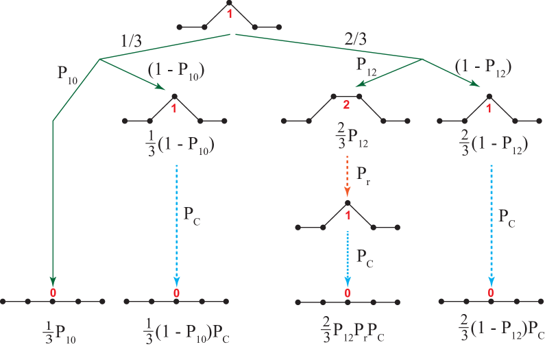
Figure 16: Event diagram for calculating the survival probability of a kink pair nucleus (triangular bump) on a planar GB moving under an applied force pointing upward. The formulas on the diagram represent the probabilities of different states of the kink pair and transitions between them.

The calculation is explained on the event diagram in Fig. 16. The following notation is used. A planar GB, a triangular bump, and a two-node kink pair are referred to as states 0, 1 and 2, respectively, according to the number of nodes above ground level. These states are labeled by red numerals. The formulas represent the probabilities of different states and transitions (jumps) between the states. The applied force is pointing upward, and the initial state of the system is a triangular bump (state 1) shown on top of the diagram. Only nodes belonging to the kinks are allowed to jump and only in a manner that preserves the single-layer height of all kinks above the ground.

It is convenient to describe the system evolution as occurring during a KMC simulation. At the first KMC step, one of the three nodes of the triangular bump is selected at random. The subsequent events are represented by the solid green arrows (Fig. 16). The tip node is selected with a probability 1/3. Once selected, the tip node can jump down with the probability $P_{10}$ or remain intact with the probability $(1-P_{10})$. If the jump attempt is successful, the triangular bump disappears. The probability of this outcome is $(1/3)P_{10}$. If the attempt fails, the triangular bump survives the first KMC step with the probability $(1/3)(1-P_{10})$. In this case, the bump can still collapse during the subsequent evolution with the (still unknown) probability $P_{c}$. This collapse can happen after a chain of jumps shown on the diagram by the dashed blue arrow. The collapse probability of the triangular bump along this route is $(1/3)(1-P_{10})P_{c}$.

Returning to the first KMC step, there is a 2/3 chance that one of the two base nodes of the triangular bump is selected. This node will then attempt to jump upward and create a two-node kink pair (state 2). The success probability of this jump is $P_{12}$, so a two-node kink pair can form with the probability of $(2/3)P_{12}$. Once formed, this kink pair can grow further or transform back into a triangular bump. The back transformation can happen immediately (probability $P_{21}$) or after some period of growth represented by the dashed red arrow. Let $P_{r}$ be the probability of returning into the triangular bump. The latter can then collapse into a planar GB. The collapse probability along this route is thus $(2/3)P_{12}P_{r}P_{c}$. Finally, if the selected base node cannot make a successful jump, the triangular bump remains but eventually collapses into a planar GB with the probability $(2/3)(1-P_{12})P_{c}$.

The bottom row on the diagram (Fig. 16) summarizes the probabilities of disappearance of the initial triangular bump along the four different routes. Since their sum must be equal to $P_{c}$, we have the equation

$$P_{c}=\dfrac{1}{3}P_{10}+\dfrac{1}{3}(1-P_{10})P_{c}+\dfrac{2}{3}P_{12}P_{r}P_{c}+\dfrac{2}{3}(1-P_{12})P_{c},$$

which is solved for $P_{c}$:

$$P_{c}=\dfrac{P_{10}}{P_{10}+2P_{12}(1-P_{r})}.$$ (48)

The remaining unknown is the return probability $P_{r}$. The problem of finding $P_{r}$ can be formulated as follows. A kink pair attempts to grow starting from a two-node state. The growth can be described as a driven random walk of the number of nodes in the pair starting from two. At each step, the number of nodes can increase by one with the probability $P_{12}$, decrease by one with the probability $P_{21}<P_{12}$, or not change. We must find the probability that the kink pair eventually collapses into a single-node state (triangular bump). This problem is equivalent to the cliff-hanger problem of a man making random steps starting one step away from a cliff (Mosteller-1965, ). The probabilities of steps away and towards the cliff are $p>1/2$ and $(1-p)<1/2$, respectively. The known solution of this problem is that the probability of falling off the cliff is $(1-p)/p$ (Mosteller-1965, ). This solution maps onto our kink pair problem by identifying $p=P_{12}/(P_{12}+P_{21})$. It follows that

$$P_{r}=\dfrac{P_{21}}{P_{12}}.$$ (49)

Inserting this solution into Eq.(48), we obtain

$$P_{c}=\dfrac{P_{10}}{P_{10}+2(P_{12}-P_{21})},$$ (50)

and thus

$$P_{s}=1-P_{r}=\dfrac{2(P_{12}-P_{21})}{P_{10}+2(P_{12}-P_{21})},$$ (51)

which is Eq.(32) of the main text.

Equation (50) was verified by independent KMC simulations implementing the process presented in Fig. 16.

Variable	Physical	Normalized
Coordinates	$x$, $z$	$\xi=x/a$, $\varsigma=z/a$
Time	$t$	$\tau=t\nu_{0}$
Velocity	$v$	$\eta=v/a\nu_{0}$
Temperature	$T$	$\theta=k_{B}T/E_{0}$
Driving force	$F$	$\varphi=Fa/E_{0}$
GB energy	$\gamma$	$\sigma=\gamma a^{2}/E_{0}$
GB stiffness	$\Lambda$	$\lambda=\Lambda a^{2}/E_{0}$
Mean squared GB width	$\overline{w^{2}}$	$\overline{\omega^{2}}=\overline{w^{2}}/a^{2}$

Table 1: Physical and normalized (dimensionless) variables in the 2D GB model.

(a)

(b)

(c)

Figure 2: Typical interface shapes at $\sigma=1$. (a) Smooth interface ($\theta=0.083$); (b) Moderately rough interface ($\theta=0.095$); (c) Fully rough interface ($\theta=0.285$). The GB is composed of $N=1024$ nodes.

(a)

(a)

(a)

Figure 10: Demonstration of dynamic GB roughening at the temperature of $\theta=0.2$ without pinning. The initially smooth GB ($\sigma=5$) remains smooth under a force of $\varphi=0.2$ (a) but becomes rough at $\varphi=4$ (b). The initially rough boundary ($\sigma=0.1$) remains equally rough at $\varphi=0.2$ (c) but becomes much rougher at $\varphi=4$ (d). The system size is $N=512$. Note the difference in the scale of the $\varsigma$-axes.

(a)

(a)

(a)

References

- (1) A. P. Sutton and R. W. Balluffi. Interfaces in Crystalline Materials. Clarendon Press, Oxford, (1995).
- (2) J. W. Cahn. The impurity-drag effect in grain boundary motion. Acta Metall. 10 (1962) 789–798.
- (3) K. Lücke and H. P. Stüwe. On the theory of grain boundary motion. In: L. Himmel, ed., Recovery and Recrystallization of Metals. Interscience Publishers, New York, 1963 171–210.
- (4) K. Lücke and H. P. Stüwe. On the theory of impurity controlled grain boundary motion. Acta Metall. 19 (1971) 1087–1099.
- (5) M. I. Mendelev, D. J. Srolovitz and W. E. Grain-boundary migration in the presence of diffusing impurities: simulations and analytical models. Philos. Mag. 81 (2001) 2243–2269.
- (6) M. I. Mendelev and D. J. Srolovitz. Impurity effects on grain boundary migration. Model. Simul. Mater. Sci. Eng. 10 (2002) R79–R109.
- (7) N. Ma, S. A. Dregia and Y. Wang. Solute segregation transition and drag force on grain boundaries. Acta Mater. 51 (2003) 3687–3700.
- (8) K. Grönhagen and J. Agren. Grain-boundary segregation and dynamic solute drag theory — A phase-field approach. Acta Mater. 55 (2007) 955–960.
- (9) F. Abdeljawad, P. Lu, N. Argibay, B. G. Clark, B. L. Boyce and S. M. Foiles. Grain boundary segregation in immiscible nanocrystalline alloys. Acta Mater. 126 (2017) 528–539.
- (10) S. G. Kim and Y. B. Park. Grain boundary segregation, solute drag and abnormal grain growth. Acta Mater. 56 (2008) 3739–3753.
- (11) J. Li, J. Wang and G. Yang. Phase field modeling of grain boundary migration with solute drag. Acta Mater. 57 (2009) 2108–2120.
- (12) M. Greenwood, C. Sinclair and M. Militzer. Phase field crystal model of solute drag. Acta Mater. 60 (2012) 5752–5761.
- (13) S. Shahandeh, M. Greenwood and M. Militzer. Friction pressure method for simulating solute drag and particle pinning in a multiphase-field model. Model. Simul. Mater. Sci. Eng. 20 (2012) 065008.
- (14) A. T. Wicaksono, C. W. Sinclair and M. Militzer. A three-dimensional atomistic kinetic Monte Carlo study of dynamic solute-interface interaction. Model. Simul. Mater. Sci. Eng. 21 (2013) 085010.
- (15) H. Sun and C. Deng. Direct quantification of solute effects on grain boundary motion by atomistic simulations. Comp. Mater. Sci. 93 (2014) 137–143.
- (16) M. J. Rahman, H. S. Zurob and J. J. Hoyt. Molecular dynamics study of solute pinning effects on grain boundary migration in the aluminum magnesium alloy system. Metall. Mater. Trans. A 47 (2016) 1889–1897.
- (17) Y. Mishin. Solute drag and dynamic phase transformations in moving grain boundaries. Acta Mater. 179 (2019) 383–395.
- (18) R. Koju and Y. Mishin. Direct atomistic modeling of solute drag by moving grain boundaries. Acta Mater. 198 (2020) 111–120.
- (19) M. Alkayyali and F. Abdeljawad. Grain boundary solute drag model in regular solution alloys. Physical Review Letters 127 (2021) 175503.
- (20) R. K. Koju and Y. Mishin. The role of grain boundary diffusion in the solute drag effect. Nanomaterials 11 (2021) 2348.
- (21) A. Suhane, D. Scheiber, M. Popov, V. I. Razumovskiy, L. Romaner and M. Militzer. Solute drag assessment of grain boundary migration in Au. Acta Materialia 224 (2022) 117473.
- (22) R. H. Swendsen. Monte Carlo studies of the interface roughening transition. Phys. Rev. B 15 (1977) 5421–5431.
- (23) C. Rottman. Roughening of low-angle grain boundaries. Phys. Rev. Lett. 57 (1986) 735–738.
- (24) D. L. Olmsted, S. M. Foiles and E. A. Holm. Grain boundary interface roughening transition and its effect on grain boundary mobility for non-faceting boundaries. Scripta Mater. 57 (2007) 1161–1164.
- (25) C. Baruffi and W. A. Curtin. Theory of spontaneous grain boundary roughening in high entropy alloys. Acta Materialia 234 (2022) 118011.
- (26) Y. Mishin. Submitted as Part I of this work.
- (27) J. Lapujoulade. The roughening of metal surfaces. Surface Science Reports 20 (1994) 195–249.
- (28) M. Hasenbusch, S. Meyer and M. Pütz. The roughening transition of the three-dimensional Ising interface: A Monte Carlo study. Journal of Statistical Physics 85 (1996) 383–401.
- (29) D. P. Landau and K. Binder. A Guide to Monte Carlo Simulations in Statistical Physics. Cambridge University Press, Cambridge, UK, third edition, (2009).
- (30) G. H. Vineyard. Frequency factors and isotope effects in solid state rate processes. Journal of Physics and Chemistry of Solids 3 (1957) 121–127.
- (31) J. W. Cahn and F. R. N. Nabarro. Thermal activation under shear. Philosophical Magazine A 81 (2001) 1409–1426.
- (32) A. H. Cottrell. Thermally activated plastic glide. Philosophical Magazine Letters 82 (2002) 65–70.
- (33) V. A. Ivanov and Y. Mishin. Dynamics of grain boundary motion coupled to shear deformation: An analytical model and its verification by molecular dynamics. Phys. Rev. B 78 (2008) 064106.
- (34) D. Chachamovitz and D. Mordehai. The stress-dependent activation parameters for dislocation nucleation in molybdenum nanoparticles. Scientific Reports 8 (2018) 3915.
- (35) J. P. Hirth and J. Lothe. Theory of Dislocations. Wiley, New York, second edition, (1982).
- (36) Y. Saito. Statistical Physics of Crystal Growth. World Scientific, Singapore, (1996).
- (37) M. P. Gelfand and M. E. Fisher. Finite-size effects in fluid interfaces. Physica A: Statistical Mechanics and its Applications 166 (1990) 1–74.
- (38) M. I. Mendelev and D. J. Srolovitz. Kink model for extended defect migration in the presence of diffusing impurities: theory and simulation. Acta Materialia 49 (2001) 2843–2852.
- (39) M. I. Mendelev and D. J. Srolovitz. Domain wall migration in 3-d in the presence of diffusing impurities. Interface Science 10 (2002) 243–250.
- (40) U. Bertocci. The influence of step motion and two-dimensional nucleation on the rate of crystal growth: Some computer simulated experiments. Surface Science 15 (1969) 286–302.
- (41) A. Seeger. The kink picture of dislocation mobility and dislocation-point-defect interactions. Journal de Physique 42 (C5) (1981) 201–228.
- (42) M. K. Chari. On reversible semi-Markov processes. Operations Research Letters 15 (1994) 157–161.
- (43) C. Maes, K. Netočný and B. Wynants. Dynamical fluctuations for semi-Markov processes. Journal of Physics A: Mathematical and Theoretical 42 (2009) 365002.
- (44) S.-Z. Yu. Hidden semi-Markov models. Artificial Intelligence 174 (2010) 215–243.
- (45) S. Balibar, F. Gallet and E. Rolley. The dynamic roughening of crystals. Journal of Crystal Growth 99 (1990) 46–53.
- (46) U. Tartaglino and A. C. Levi. Dynamic roughening: Nucleation and stochastic equations. Physica A: Statistical Mechanics and its Applications 277 (2000) 83–105.
- (47) S.-J. L. KANG, S.-Y. KO and S.-Y. MOON. Mixed control of boundary migration and the principle of microstructural evolution. Journal of the Ceramic Society of Japan 124 (2016) 259–267.
- (48) J. Marian, W. Cai and V. V. Bulatov. Dynamic transitions from smooth to rough to twinning in dislocation motion. Nature Materials 3 (2004) 158–163.
- (49) J. W. Cahn, Y. Mishin and A. Suzuki. Coupling grain boundary motion to shear deformation. Acta Mater. 54 (2006) 4953–4975.
- (50) T. Frolov and Y. Mishin. Thermodynamics of coherent interfaces under mechanical stresses. II. Application to atomistic simulation of grain boundaries. Phys. Rev. B 85 (2012) 224107.
- (51) T. Frolov, D. L. Olmsted, M. Asta and Y. Mishin. Structural phase transformations in metallic grain boundaries. Nature Communications 4 (2013) 1899.
- (52) J. Hickman and Y. Mishin. Disjoining potential and grain boundary premelting in binary alloys. Phys. Rev. B 93 (2016) 224108.
- (53) J. Hickman and Y. Mishin. Extra variable in grain boundary description. Phys. Rev. Materials 1 (2017) 010601.
- (54) T. Frolov, M.Asta and Y. Mishin. Segregation-induced phase transformations in grain boundaries. Phys. Rev. B 92 (2015) 020103(R).
- (55) C. P. Race, J. von Pezold and J. Neugebauer. Role of the mesoscale in migration kinetics of flat grain boundaries. Phys. Rev. B 89 (2014) 214110.
- (56) C. P. Race, R. Hadian, J. von Pezold, B. Grabowski and J. Neugebauer. Mechanisms and kinetics of the migration of grain boundaries containing extended defects. Phys. Rev. B 92 (2015) 174115.
- (57) R. Hadian, B. Grabowski, C. P. Race and J. Neugebauer. Atomistic migration mechanisms of atomically flat, stepped, and kinked grain boundaries. Physical Review B 94 (2016) 165413.
- (58) E. R. Homer, O. K. Johnson, D. Britton, J. E. Patterson, E. T. Sevy and G. B. Thompson. A classical equation that accounts for observations of non-Arrhenius and cryogenic grain boundary migration. npj Computational Materials 8 (2022) 157.
- (59) Y. Mishin. Thermodynamic theory of equilibrium fluctuations. Annals of Physics 363 (2015) 48–97.
- (60) F. Mosteller. Fifty Challenging problems in probability with solutions. Dover books on mathematics. Dover, p. 51-54, (1987).