Stochastic model and kinetic Monte Carlo simulation of solute interactions with stationary and moving grain boundaries. I. Model formulation and application to one-dimensional systems

Abstract

A simple stochastic model of solute drag by moving grain boundaries (GBs) is presented. Using a small number of parameters, the model describes solute interactions with GBs and captures nonlinear GB dynamics, solute saturation in the segregation atmosphere, and the breakaway from the atmosphere. The model is solved by kinetic Monte-Carlo (KMC) simulations with time-dependent transition barriers. The non-Markovian nature of the KMC process is discussed. In Part I of this work, the model is applied to planar GBs driven by an external force. The model reproduces all basic features of the solute drag effect, including the maximum of the drag force at a critical GB velocity. The force-velocity functions obtained depart from the scaling predicted by the classical models by Cahn and Lücke-Stüwe, which are based on more restrictive assumptions. The paper sets the stage for Part II, in which the GB will be treated as a 2D solid-on-solid interface.

I Introduction

Many properties of technological materials are controlled by the motion, or resistance to the motion, of grain boundaries (GBs) under the action of capillarity and other thermodynamic driving forces (Balluffi95, ). In alloys, the interaction of GBs with alloy components can drastically reduce the GB mobility due to the solute drag effect. This effect has been studied experimentally, theoretically, and by computer simulations for decades. The first quantitative model of the solute drag was proposed by Cahn (Cahn-1962, ) and Lücke et al. (Lucke-Stuwe-1963, ; Lucke:1971aa, ). Their model predicts a highly nonlinear relation between the GB velocity and the drag force. The drag force exhibits a maximum separating two kinetic regimes. In the low-velocity regime, the GB drags the solute segregation atmosphere. In the high-velocity regime, the boundary breaks away from the atmosphere but soon forms a new, lighter atmosphere that poses less resistance to the GB motion.

On the computational side, the solute drag was studied by the phase field (Wang03, ; Li:2009aa, ; Shahandeh:2012aa, ; Gronhagen:2007aa, ; Abdeljawad:2017aa, ; Alkayyali:2021uo, ) and phase-field crystal (Greenwood:2012aa, ) methods, and by molecular (MD) simulations (Mendelev02a, ; Sun:2014aa, ; Wicaksono:2013aa, ; Mendelev:2001aa, ; Rahman:2016aa, ; Kim:2008aa, ). MD offers the most powerful approach to studying the solute drag. It provides access to all atomic-level details of the GB motion and does not rely on any assumptions or approximations other than those built into the interatomic potential. However, the timescale of MD simulations is presently limited to about a hundred nanoseconds, which is too short for reliable modeling of diffusion in the lattice by the vacancy mechanism. Despite this limitation, recent work (Koju:2020aa, ; Koju:2021aa, ) has shown that the “short circuit” GB diffusion and the cloud of non-equilibrium vacancies surrounding the moving boundary provide sufficient diffusion mobility to observe the solute drag on the MD time scale. Significant insights into the solute drag mechanisms were obtained, especially regarding the role of the in-plane GB diffusion. Presently, such simulations remain very challenging. They heavily rely on computational power and depend on the availability and reliability of interatomic potentials for alloy systems.

In this work, we approach the solute drag problem from a different direction. Our goal is to create a minimalist model that would be as simple as possible and only depend on a small number of parameters but would still capture the most essential physics of the solute drag effect. The model proposed here is stochastic and is solved by kinetic Monte Carlo (KMC) simulations. The paper is divided into two parts. In Part I, we introduce our model and demonstrate its first application. Section II describes the kinetic theory underlying the model and its KMC implementation. In section III, we specialize the model to GB motion in one-dimensional (1D) systems. We show that the model reproduces all basic features of the solute drag effect, including the maximum of the force-velocity function predicted by the classical models (Cahn-1962, ; Lucke-Stuwe-1963, ; Lucke:1971aa, ). However, the model departs from the scaling predicted by the classical models as it captures more realistic GB dynamics. In Part II (Mishin_2023_RW_part_II, ), we will present a 2D version of the model, which treats the GB as a solid-on-solid interface with an adjustable interface energy and reproduces a GB roughening transition in both stationary and moving boundaries. This will allow us to study the dynamic roughening phenomenon and its impact on GB migration mechanisms and the solute drag.

II The kinetic model

II.1 Random walk without pinning

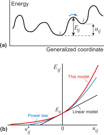
Figure 1: (a) Schematic 1D representation of energy landscape of a system capable of jumping between energy minima by thermal fluctuations. $E_{ij}$ is the energy barrier from state $i$ to state $j$ with energies $u_{i}$ and $u_{j}$, respectively. (b) Energy barrier as a function of energy difference $u_{ij}=u_{j}-u_{i}$ in the present model compared with the linear and power-law models.

Consider a system whose potential energy surface has a set of local minima. The system is coupled to a thermostat at a temperature $T$ and can transition between the energy minima by thermal fluctuations (Fig. 1(a)). We further assume that such transitions (jumps) only occur between states separated by a single energy barrier. We adopt the harmonic transition state theory (TST) (Vineyard:1957vo, ), by which the transition rate $\omega_{ij}$ from state $i$ to state $j$ is given by

$$\omega_{ij}=\nu_{0}\exp\left(-\dfrac{E_{ij}}{k_{B}T}\right),$$ (1)

where $E_{ij}$ is the transition barrier, $k_{B}$ is Boltzmann’s constant, and $\nu_{0}$ is the attempt frequency. For simplicity, $\nu_{0}$ is assumed to be the same for all transitions.

The following rule is introduced for the transition barriers:

$$E_{ij}=\begin{cases}E_{0}\exp\left(\dfrac{u_{ij}}{2E_{0}}\right),&u_{ij}\leq 0,\\ u_{ij}+E_{0}\exp\left(-\dfrac{u_{ij}}{2E_{0}}\right),&u_{ij}>0,\end{cases}$$ (2)

where $u_{ij}=u_{j}-u_{i}$ is the energy difference between initial ($u_{i}$) and destination ($u_{j}$) states, and $E_{0}$ is the barrier between the states of equal energy ($u_{i}=u_{j}$). According to Eq.(2), transition barriers to lower (higher) energy states are lower (higher) than $E_{0}$. Generally, the barrier is a nonlinear function of $u_{ij}$ (Fig. 1(b)). However, if the energy difference is small, $\left|u_{ij}\right|\ll E_{0}$, then the barrier can be approximated by $E_{ij}=E_{0}+u_{ij}/2$. This linear approximation is often employed to describe weakly driven systems. If the energy difference is large ($\left|u_{ij}\right|\gg E_{0}$), then the barrier is large and close to $u_{ij}$ for transitions to higher-energy states and exponentially small for transitions to lower-energy states.

Previous energy-barrier models assumed that, under a sufficiently large energy difference $-u_{ij}$, the barrier is suppressed to zero at a critical value $u_{ij}^{*}$. It was further assumed that the barrier follows the power law $E_{ij}\propto\left(u_{ij}-u_{ij}^{*}\right)^{\alpha}$ at $u_{ij}\gtrsim u_{ij}^{*}$ and remains strictly zero at $u_{ij}<u_{ij}^{*}$. Theoretical models predict the critical exponent $\alpha=3/2$ (Cahn:2001wh, ; Cottrell:2002ub, ; Ivanov08a, ), although computer simulations often deviate from this value (Chachamovitz:2018vm, ). In the present model, the zero-barrier point is regularized by replacing the power law with an exponential decay of the barrier with increasing $\left|u_{ij}\right|$. The exponential decay ensures that the barrier remains positive under any driving force. This regularization is introduced for computational convenience and does not affect any physically meaningful results. Indeed, the TST underlying Eq.(1) is only valid when $E_{ij}\gg k_{B}T>0$. Any results obtained at $E_{ij}\rightarrow 0$ lie outside the validity domain of the TST and must be ignored in all applications of this model.

If the system is confined to a finite-size domain in the configuration space, it eventually reaches a state of dynamic equilibrium. Note that the energy-barrier relation (2) satisfies the detailed balance condition

$$\omega_{ij}\exp\left(-\dfrac{u_{i}}{k_{B}T}\right)=\omega_{ji}\exp\left(-\dfrac{u_{j}}{k_{B}T}\right),$$ (3)

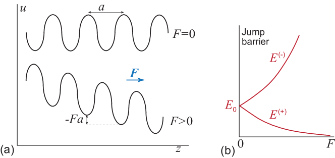
Figure 2: (a) Schematic energy landscape of a 1D periodic system before and after application of a spatially uniform external force $F>0$. (b) The force suppresses the energy barrier $E^{(+)}$ for forward jumps and raises the barrier $E^{(-)}$ for backward jumps relative to the unbiased barrier $E_{0}$.

where the exponential terms represent the Boltzmann probabilities of finding the system in the respective states. On the other hand, an open system subjected to a driving force executes a driven random walk and never reaches equilibrium. This is illustrated in Figure 2 by a 1D example in which a uniform driving force $F>0$ tilts the periodic energy landscape of the system and changes the initial barrier $E_{0}$ to

$$E^{(+)}=E_{0}\exp\left(-\dfrac{Fa}{2E_{0}}\right)$$ (4)

for forward jumps and

$$E^{(-)}=Fa+E_{0}\exp\left(-\dfrac{Fa}{2E_{0}}\right)$$ (5)

for backward jumps ($a$ being the energy period). The bias between the forward and backward barriers causes a drift of the system in the force direction with the velocity

$$v=a\nu_{0}\left[\exp\left(-\dfrac{E^{(+)}}{k_{B}T}\right)-\exp\left(-\dfrac{E^{(-)}}{k_{B}T}\right)\right].$$ (6)

The system evolution can be modeled by KMC simulations implementing a sequence of jump attempts that may or may not be successful. We assume for simplicity that each state has the same number $m$ of available escape routes. At each step of the KMC process, a random number $r_{1}\in[0,1)$ chooses one of the possible jumps $i\rightarrow j$ from the current state $i$ with equal probability. Then another random number $r_{2}\in[0,1)$ decides if the chosen jump attempt is successful. The jump is implemented if $r_{2}<p_{ij}$, where

$$p_{ij}=\exp\left(-\dfrac{E_{ij}}{k_{B}T}\right)$$ (7)

is the success probability; otherwise the attempt fails. In either case, the clock is advanced by $\Delta t=\left(m\nu_{0}\right)^{-1}$ and the process repeats. $m$ KMC steps correspond to one physical attempt with the frequency $\nu_{0}$.

II.2 The pinning effect

The previous discussion assumed that the energy landscape of the system and the unbiased barrier $E_{0}$ were fixed. We will now modify this assumption. Let us first consider unbiased jumps ($u_{i}=u_{j}$). After each unsuccessful attempt, we will penalize the system by increasing the jump barriers for all escape routes. After $n$ unsuccessful attempts, the barriers become

$$E_{t}=E_{0}\left(1+(\alpha-1)\dfrac{\sqrt{t/t_{p}}}{1+\sqrt{t/t_{p}}}\right),$$ (8)

where $t=n\Delta t$ is the discrete time variable, and $\alpha>1$ and $t_{p}>0$ are model parameters. The first attempt ($t=0$) uses the unpenalized barriers $E_{0}$. If this attempt fails, the barriers for the second attempt become $E_{1}>E_{0}$. If the second attempt is also unsuccessful, the barriers become $E_{2}>E_{1}$, and so on. As long as $t\ll t_{p}$, the barriers grow with time as $\sqrt{t}$. In the limit of $t\gg t_{p}$, the barriers plateau at

$$E_{\infty}=\alpha E_{0}>E_{0}.$$ (9)

After the system finally makes a successful jump, the attempt counter $n$ is reset to zero and the process repeats from the new state.

In the presence of energy gradients ($u_{i}\neq u_{j}$), the jump barriers are given by Eq.(2) with $E_{0}$ replaced by $E_{t}$ from Eq.(8).

The physical motivation for introducing the time-dependent barriers is to describe the GB interaction with solute atoms, including the solute drag effect (Cahn-1962, ; Lucke-Stuwe-1963, ; Lucke:1971aa, ). The amount of solute transported to the boundary by diffusion initially increases as the square root of time, reflecting diffusion kinetics. The solute atoms form a segregation atmosphere that reduces the boundary mobility by raising the energy barriers for its random displacements. After the segregation atmosphere has reached its maximum capacity (saturation), the barriers remain constant. This behavior is captured by Eq.(8), which ensures that $E_{t}$ grows as $\sqrt{t}$ at $t\ll t_{p}$ and reaches a plateau value $E_{\infty}$ in the long-time limit ($t\gg t_{p}$).

In addition to the solute drag by moving GBs, this model is relevant to the motion of other crystalline defects in the presence of segregating chemical components reducing the defect mobility. The defect in question can be a lattice dislocation whose mobility is slowed down by a Cottrell atmosphere of solute atoms (Hirth, ; Cottrell:1948aa, ; Cottrell_Bilby, ; Cottrell:1953aa, ). As another example, consider diffusion of slow impurity atoms in the presence of highly mobile atoms of another chemical component that interacts with the impurity atoms creating a short-range order around them. This short-range order can be treated as a segregation atmosphere reducing the impurity mobility.

For brevity, the increase in the jump barriers with time will be referred to as the “pinning” effect. This term should not be understood as literally pinning the system in place. It only refers to the retardation of the system dynamics caused by the diffusion-controlled formation of a segregation atmosphere. Accordingly, the parameter $t_{p}$ will be called the pinning time. The latter is related to the solute diffusion coefficient $D$ by

$$D=\dfrac{a^{2}}{t_{p}}=\dfrac{t_{0}}{t_{p}}D_{0}.$$ (10)

Here, $a$ is a characteristic jump length, $D_{0}=a^{2}/t_{0}$ is the intrinsic diffusivity of the unpinned system executing a random walk by thermal fluctuations, and

$$t_{0}=\dfrac{1}{m\nu_{0}}\exp\left(\dfrac{E_{0}}{k_{B}T}\right)$$ (11)

is the unpinned and unbiased residence time of the system. Likewise, $E_{\infty}$ has the meaning of the fully pinned jump barrier. The difference $(E_{0}-E_{\infty})=(1-\alpha)E_{0}<0$ can be interpreted as the solute binding energy to the system. Accordingly, $\alpha$ will be called the pinning factor of the solute atoms.

Note the simplicity of the proposed model. The input information consists of five parameters: the jump length $a$, the TST parameters $\nu_{0}$ and $E_{0}$, and the pinning parameters $t_{p}$ and $\alpha$. All other variables mentioned above, such as $t_{0}$, $E_{\infty}$, and $D$, can be expressed through the five independent parameters $(a,\nu_{0},E_{0},t_{p},\alpha)$. With this limited input, the model can be solved by KMC simulations to describe the dynamics of the driven system. This simple model captures the main physics of the solute drag effect as will be demonstrated later in the paper and in Part II (Mishin_2023_RW_part_II, ).

III 1D model of solute drag

III.1 GB random walk without pinning

As the first application, we will consider 1D random walk of a system on the $z$ axis as depicted in Fig. 2. The energy landscape is periodic with a period $a$. This model represents a planar GB driven by an external force. Note that the classical models by Cahn and Lücke (Cahn-1962, ; Lucke-Stuwe-1963, ; Lucke:1971aa, ) also treat the GB as a planar interface and are essentially 1D models.

In the absence of driving forces and pinning, the GB executes an unbiased random walk with the jump length $a$ and the barrier $E_{0}$. The escape probability per physical attempt is

$$p_{0}=2\exp\left(-\dfrac{E_{0}}{k_{B}T}\right),$$ (12)

where the factor of two takes into account that the GB can escape by either a forward or a backward jump ($m=2$). The residence time of the GB is a discrete stochastic variable $n\nu_{0}^{-1}$, where $n=1,2,...$ is a counter of attempts. Since the attempts are statistically independent, the escape probability after $n$ unsuccessful attempts follows the geometric distribution

$$\mathsf{P}(n)=p_{0}(1-p_{0})^{n}.$$ (13)

In the long-time limit ($n\gg 1/p_{0}$), this distribution becomes exponential,

$$\mathsf{P}(n)=p_{0}e^{-p_{0}n}.$$ (14)

It can be shown that the expectation value of the residence time is

$$t_{0}=\dfrac{1}{\nu_{0}p_{0}}=\dfrac{1}{2\nu_{0}}\exp\left(\dfrac{E_{0}}{k_{B}T}\right).$$ (15)

Now suppose a driving force $F>0$ is applied to the GB. The force reduces the forward jump barrier and raises the backward jump barrier according to Eqs.(4)-(5); see also Figure 2. This bias causes a drift of the GB with the velocity given by Eq.(6). When the force is small ($F\ll E_{0}/a$), the barriers are approximately linear in the force, $E^{(\pm)}=E_{0}\mp Fa/2$, and Eq.(6) predicts the linear dynamics

$$v=MF,$$ (16)

where

$$M=\dfrac{a^{2}\nu_{0}}{k_{B}T}\exp\left(-\dfrac{E_{0}}{k_{B}T}\right)$$ (17)

is the GB mobility. A medium force ($F\approx E_{0}/a$) causes an upward deviation from the linear law. In the large-force limit ($F\gg E_{0}/a$), the velocity slows down and follows the asymptotic relation

$$v=a\nu_{0}\exp\left(-{\displaystyle\dfrac{E_{0}\exp\left(-\dfrac{Fa}{2E_{0}}\right)}{k_{B}T}}\right).$$ (18)

The upper bound of the GB velocity is $a\nu_{0}$ but this velocity is never reached because the barrier never becomes strictly zero. The physical motivation for preventing a zero barrier is that the GB jumps are accompanied by energy dissipation in the form of phonon drag and, in alloys, the solute drag. The model attempts to capture the dissipation effects by keeping the barrier positive even under a strong force. It should also be noted that Eq.(18) is physically meaningful only as long as the numerator in the exponent is $\gg k_{B}T$; otherwise the TST cannot be applied.

III.2 GB random walk with pinning

We next consider unbiased ($F=0$) GB walk with pinning. Unsuccessful jump attempts are now penalized according to Eq.(8). For a fully pinned GB ($E_{t}\approx E_{\infty}$), the escape probability per physical attempt is

$$p_{\infty}=2\exp\left(-\dfrac{E_{\infty}}{k_{B}T}\right),$$ (19)

and the number of failed attempts follows the geometric distribution

$$\mathsf{P}(n)=p_{\infty}(1-p_{\infty})^{n}.$$ (20)

In the large-$n$ limit, this distribution converges to exponential,

$$\mathsf{P}(n)=p_{\infty}e^{-p_{\infty}n},$$ (21)

and the expectation value of the residence time becomes

$$t_{\infty}=\dfrac{1}{\nu_{0}p_{\infty}}=t_{0}\exp\left(\dfrac{E_{\infty}-E_{0}}{k_{B}T}\right)=t_{0}\exp\left(\dfrac{(\alpha-1)E_{0}}{k_{B}T}\right).$$ (22)

If the pinning time is long ($t_{p}\gg t_{0}$), the atmosphere formation is a slow process. Then there is a high probability that the GB escapes before any significant atmosphere can form. The pinning has little effect on the GB walk. This is the case for slow solute diffusion ($D\ll D_{0}$). If $t_{p}\ll t_{0}$, a fully saturated atmosphere forms before the GB has a chance to escape. Accordingly, the jump barrier is close to $E_{\infty}$ and the residence time is close to $t_{\infty}$. This is the case when the solute diffusion is fast ($D\gg D_{0}$). On the intermediate time scale between the two limits ($t_{p}\approx t_{0}$), the residence time no longer follows the geometric or exponential distribution, making the process non-Markovian. The expectation value of the residence time lies between $t_{0}$ and $t_{\infty}$. We call this kinetic regime “active pinning”.

We next apply a driving force $F>0$ causing the GB to drift in the positive $z$ direction. This drift cannot be described analytically and was studied by KMC simulations. The simulations were performed in dimensionless variables using $a$, $\nu_{0}^{-1}$ and $k_{B}T$ as the units of length, time, and energy, respectively. All KMC results reported below are for $t_{0}\nu_{0}=50$ and thus $E_{0}/k_{B}T=4.6$. These values were chosen as a compromise between computational efficiency and the $E_{0}/k_{B}T\gg 1$ requirement of the TST.

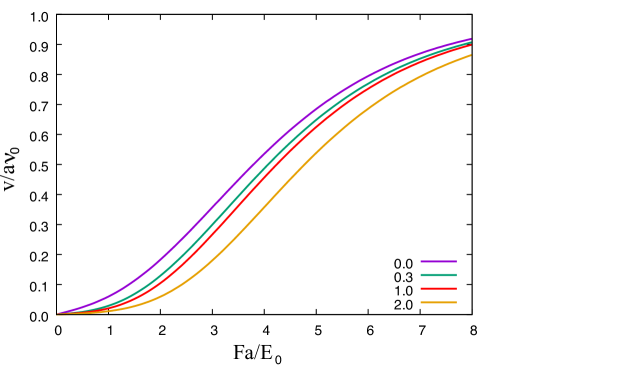
(b)

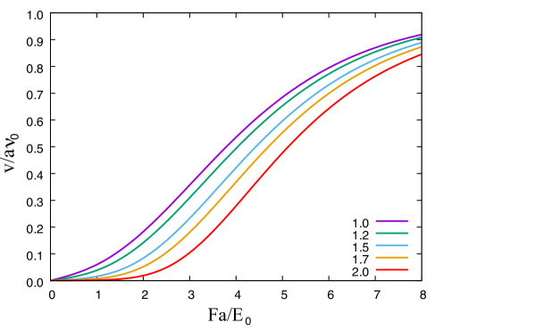
Figure 3: Velocity-force relations for: (a) several normalized solute diffusivities $D/D_{0}$ indicated in the key at a fixed pinning factor $\alpha=1.5$; (b) several $\alpha$ values indicated in the key at a fixed $D/D_{0}=2.0$.

Figure 3(a) shows the velocity-force functions for a series of normalized solute diffusivities $D/D_{0}$ with a fixed pinning factor $\alpha=1.5$. Figure 3(b) shows such functions for a series of $\alpha$ values with a fixed $D/D_{0}=2.0$. As expected, the results for $D/D_{0}=0$ (no solute diffusion) and $\alpha=1$ (no solute segregation) perfectly match the analytical solution (6) (not shown in the figure). The plots demonstrate that increasing the solute diffusivity and/or the pinning factor reduces the GB velocity under a given driving force, which is a manifestation of the solute drag effect.

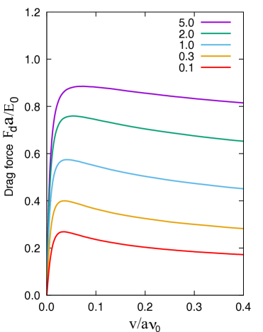
(a)  (b)

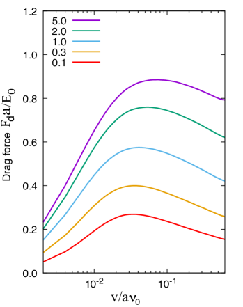
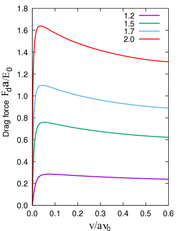
(c)  (d)

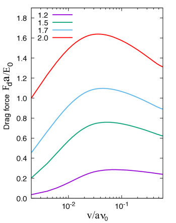
Figure 4: Solute drag force as a function of velocity for: (a,b) several normalized solute diffusivities $D/D_{0}$ indicted in the key at a fixed pinning factor $\alpha=1.5$; (c,d) several $\alpha$ values indicted in the key at a fixed $D/D_{0}=2.0$. Panels (b) and (d) use the logarithmic velocity scale to better reveal the drag-breakaway transition.

The solute drag force $F_{d}$ is the difference between the force required to drive a segregated GB and the force to drive an unpinned GB ($D/D_{0}=0$ or $\alpha=1$) with the same velocity. The velocity dependence of the normalized solute drag force, $F_{d}a/E_{0}$, is displayed in Figs. 4(a,b) for several $D/D_{0}$ values at a fixed $\alpha=1.5$, and in Figs. 4(c,d) for several $\alpha$ values at a fixed $D/D_{0}=2.0$. In agreement with the classical models, the drag force reaches a maximum at a critical velocity $v_{*}$ separating the solute drag regime at $v<v_{*}$ and the breakaway regime at $v>v_{*}$. The transition between the two regimes occurs continuously over a wide velocity range. This transition is best revealed using the logarithmic velocity axis as in Figs. 4(b,d).

Although the observation of the two kinetic regimes is in qualitative agreement with the classical models (Cahn-1962, ; Lucke-Stuwe-1963, ; Lucke:1971aa, ), there are also significant differences. For example, Cahn’s model (Cahn-1962, ) predicts that the drag force is a function of the dimensionless parameter $av/D$ [Eqs.(16)-(8) in (Cahn-1962, )]. According to this prediction, the maximum drag force must be independent of the solute diffusivity $D$, while the peak position $v_{*}$ must be proportional to $D$. In our model, the solute diffusivity $D$ is given by Eq.(10), so Cahn’s scaling variable is $vt_{p}/a$. This variable has the meaning of the distance traveled by the moving GB during the pinning time $t_{p}$. Contrary to this prediction, the peak force obtained by the simulations sharply increases with $D$ (Figs. 4(a,b)). The peak velocity $v_{*}$ is not proportional to $D$ either. A similar lack of the $av/D$ scaling was observed in previous KMC simulations within a 2D Ising model (Mendelev:2001aa, ) and 3D solid-on-solid model (Wicaksono:2013aa, ). This discrepancy is due to the crude approximations underlying the classical models. Both our present model and Cahn’s theory (Cahn-1962, ) represent the GB by a planar interface, but our model captures the solute saturation effect missing in Cahn’s theory and explicitly treats the nonlinear GB dynamics both with and without the GB-solute interactions.

Figure 4 also shows the trend for the drag force maximum to widen with increasing solute diffusivity and/or decreasing pinning factor. Although not shown in Fig. 4, at sufficiently large $D/D_{0}$ values and/or sufficiently small $\alpha$, the maximum smooths out. The thinning of the segregation atmosphere with increasing velocity becomes a continuous process not accompanied by a breakaway event.

IV Discussion and conclusions

This work aimed to develop a minimalist model capturing the main physics of the solute drag by moving GBs. The key feature of the solute drag effect is the kinetic competition between GB migration and diffusion of the solute atoms. A moving GB, driven by an external force, tries to increase its mobility by breaking away from the solute segregation atmosphere. The formation of the atmosphere is kinetically controlled by solute diffusion. If the latter outpaces the GB migration, a heavy atmosphere forms that slows the GB down. If the GB mobility is high relative to solute diffusion, the GB only carries a light atmosphere and can move faster.

The model proposed here describes this kinetic competition. It represents both linear and nonlinear GB dynamics using only three parameters: $a$, $\nu_{0}$ and $E_{0}$. The solute interaction with the GB and the solute diffusivity are represented by two more parameters: the pinning strength $\alpha$ and the pinning time $t_{p}$. The solute diffusion is included in the model through the square root time dependence of the GB jump barriers. Out of the five parameters mentioned, $\nu_{0}$ and $a$ set the time and length scales of the problem and are unrelated to the competition of the kinetic regimes. The key parameters of the model are $E_{0}$, $\alpha$ and $t_{p}$. We believe that this model achieves the ultimate simplicity in describing the solute drag effect. Nothing in the model can be removed without losing the underlying physics.

The 1D version of the model presented in this paper reproduces the main features of the solute drag, including the drag force maximum at a critical velocity. The model predictions are in qualitative agreement with the classical models (Cahn-1962, ; Lucke-Stuwe-1963, ; Lucke:1971aa, ), which are also based on 1D geometry. However, the classical models rely on more restrictive assumptions, such as the dilute solution approximation and linear GB dynamics in the absence of solute atoms. The present model captures some of the missing features, including nonlinear dynamics and the solute saturation effect.

The introduction of time-dependent transition barriers in this model raises some theoretical questions that are not apparent in the 1D version of the model but are more relevant to the 2D version (Mishin_2023_RW_part_II, ) and other possible applications. One of the questions is whether the KMC simulations based on this model implement a Markov chain. On one hand, the GB jump probabilities from a given state are statistically independent of the previous jumps, as in a Markov chain. On the other hand, the residence time probability distribution is not exponential as it should be in a continuous-time Markov process, making our process non-Markovian. Specifically, the random walk with pinning introduced in this model can be classified as a homogeneous semi-Markov process (Chari:1994aa, ; Yu:2010aa, ). The homogeneity means that the residence time distribution depends only on the time counted from the arrival at the current state, not the absolute time. The TST requirement of relatively high escape barriers implies long residence times with many unsuccessful attempts. As such, the random walk can be treated as a continuous-time process (Yu:2010aa, ). However, in the actual simulations, the residence time cannot be too long for computational reasons. In some cases where the average number of failed attempts is not too large, the simulations implement a discrete-time semi-Markov process (Yu:2010aa, ).

Mathematical analysis of random walk with pinning is beyond the scope of this work. We are more concerned with the consequences of the non-Markovian nature of the process for the physical behavior of the system. One question is whether the random walk always converges to a unique steady state. While we cannot present a general proof that it always does, in all cases tested in this work, the KMC simulations did converge to a steady state that was independent of the initial condition. This was found for both driven processes as well as stationary states arising in a bound system in the absence of external forces. The steady-state occupation probabilities do not generally follow the Boltzmann distribution. The detailed balance condition in the form of Eq.(3) is not satisfied. However, it is accurately followed when the non-Boltzmann occupation probabilities are used to formulate the detailed balance. Given that the residence time does not correlate with the jump directions, the microscopic reversibility is also preserved (Wang:2007aa, ). Some of these features are illustrated by a simple three-level model with pinning presented in the Appendix.

Transitions between different states of GBs, dislocations, and other crystalline defects subject to active pinning are intrinsically non-Markovian, whether the system is driven by an applied force or fluctuates around a fixed average position. At best, the chains of such transitions constitute semi-Markov processes (Maes:2009aa, ). More details related to simulations of pinned systems will be discussed in Part II of this work (Mishin_2023_RW_part_II, ).

Acknowledgements

This research was supported by the National Science Foundation, Division of Materials Research, under Award no. 2103431.

Appendix: three-level system with pinning

In this Appendix, we present a toy model that illustrates some of the features of random walk in the presence of pinning.

Consider a three-level system coupled to a thermostat and subject to the pinning effect introduced in the main text. The system can spontaneously jump between the states starting from some initial condition. We can model this process by a KMC simulation. At each KMC step, two random numbers, $r_{1}$ and $r_{2}$, are generated in a unit interval. $r_{1}$ selects one of the two states, $j$, different from the current state $i$ with equal probability. Then $r_{2}$ decides if the jump $i\rightarrow j$ is implemented, depending on whether $r_{2}<p_{ij}$ (successful attempt) or $r_{2}\geq p_{ij}$ (failed attempt). Here,

$$p_{ij}=e^{-E_{ij}/\theta}$$ (23)

is the jump probability, $\theta$ is reduced temperature, and $E_{ij}$ is the $i\rightarrow j$ jump barrier. $E_{ij}$ depends on the state energies $u_{i}$ and $u_{j}$:

$$E_{ij}=\begin{cases}E_{t}\exp\left(\dfrac{u_{ij}}{2E_{t}}\right),&u_{ij}\leq 0,\\ u_{ij}+E_{t}\exp\left(-\dfrac{u_{ij}}{2E_{t}}\right),&u_{ij}>0,\end{cases}$$ (24)

where $u_{ij}=u_{j}-u_{i}$ and $E_{t}$ is the unbiased (when $u_{i}=u_{j}$) jump barrier. The latter is given by

$$E_{t}=1+(\alpha-1)\dfrac{\sqrt{\tau/\tau_{p}}}{1+\sqrt{\tau/\tau_{p}}},$$ (25)

where $\alpha>1$ is the pinning factor, $\tau_{p}$ is the pinning time, and $\tau$ is the elapsed time after the previous jump. In the KMC simulations, $\tau$ is a discrete variable equal to the number of previously failed attempts. After each successful jump, $\tau$ is reset to zero.

Note that $p_{ij}$ and $p_{ji}$ satisfy the equation

$$e^{-u_{i}/\theta}p_{ij}=e^{-u_{j}/\theta}p_{ji}.$$ (26)

This equation looks like a detailed balance relation with Boltzmann’s occupation probabilities. However, it cannot be interpreted this way because $p_{ij}$ and $p_{ji}$ are independently fluctuating variables corresponding to generally different $E_{t}$ values. Averaging over a long KMC trajectory is required for testing the detailed balance hypothesis, which will be done below.

Let us first consider two limiting cases. Suppose $\tau_{p}\gg\tau_{0}$, where $\tau_{0}$ is the unpinned and unbiased residence time,

$$\tau_{0}=\dfrac{1}{2}e^{1/\theta}.$$ (27)

Then Eq.(25) gives $E_{t}=1$ and the pinning effect is negligible. In the other limit, when $\tau_{p}\ll\tau_{0}$, $E_{t}$ increases with time in proportion to $\sqrt{\tau}$ to mimic the diffusion-controlled kinetics of the pinning process. In the $\tau_{p}/\tau_{0}\rightarrow 0$ limit, $E_{t}$ tends to $E_{\infty}=\alpha$; the system gets pinned instantly and continues to evolve with the barrier $E_{t}=E_{\infty}>1$.

In both limiting cases, the unbiased barrier $E_{t}$ is time-independent and the random walk between the states is a Markov chain. Accordingly, Eq.(26) is a true detailed balance relation with Boltzmann’s occupation probabilities. Furthermore, the unpinned and fully pinned systems must converge to the same steady state with Boltzmann’s occupation probabilities

$$c_{i}^{B}=\dfrac{1}{\mathcal{P}}e^{-u_{i}/\theta},$$ (28)

where

$$\mathcal{P}=\sum_{i}e^{-u_{i}/\theta}$$ (29)

is the partition function. The ensemble-averaged system energy is then

$$\varepsilon_{B}=\sum_{i}e^{-u_{i}/\theta}u_{i}$$ (30)

and the heat capacity is

$$C_{B}=\dfrac{d\varepsilon_{B}}{d\theta}=\dfrac{1}{\theta^{2}}\left(\dfrac{1}{\mathcal{P}}\sum_{i}u_{i}^{2}e^{-u_{i}/\theta}-\varepsilon^{2}\right).$$ (31)

Between the two extremes lies the case of active pinning in which $\tau_{p}\approx\tau_{0}$. The unbiased barrier $E_{t}$ is then stochastic and time-dependent, making the random walk a semi-Markov process. Analytical treatment of this case is challenging but we can study it by KMC simulations. The questions we seek to answer are:

• Do the simulations converge to a steady state, and if so, does the steady state depend on the initial condition?

• What are the steady-state occupation probabilities $c_{i}$ of the energy levels? Generally, they need not follow Boltzmann’s distribution (28).

• Do the energy fluctuations in the steady state follow the canonical distribution (Landau-Lifshitz-Stat-phys, ; Mishin:2015ab, )?

• When the system is in a steady state, do the jumps satisfy the detailed balance condition or only the general balance condition (Manousiouthakis:1999wn, )?

The last question requires a clarification. If the system reaches a steady state, it must satisfy at least the general balance condition (Manousiouthakis:1999wn, )

$$\sum_{j\neq i}J_{ij}=\sum_{j\neq i}J_{ji}\qquad(\mathrm{fixed\ }i)$$ (32)

for each state $i.$ Here, $J_{ij}$ is the $i\rightarrow j$ jump rate (number of $i\rightarrow j$ jumps per unit time) averaged over a long KMC trajectory. Equation (32) states that the jumps in and out of any state $i$ balance each other so that the occupation probability $c_{i}$ is time-independent. The question is whether the detailed balance relations

$$J_{ij}=J_{ji}$$ (33)

hold for all individual $(i,j)$ pairs, which is obviously a stronger condition than Eq.(32).

It should be reminded that this model only makes physical sense when $\theta\ll 1$; otherwise the transition state theory underlying Eq.(23) is invalid. We performed KMC simulations at temperatures $0.1<\theta<0.35$. Here, the upper bound attempts to meet the TST requirement while the lower bound is imposed by the computational challenge of working with high barriers. The simulation results are summarized below.

For any choice of $\theta$ and $\tau_{p}$, we find that the simulations converge to the same steady state regardless of the initial state. The detailed balance condition (33) is satisfied within the statistical scatter of the results. This is illustrated in Fig. 5(a) for a system with energy levels $u_{1}=0$, $u_{2}=0.2$, and $u_{3}=0.4$ at the temperature of $\theta=0.2$. The plot shows that the detailed balance is followed in the unpinned, fully pinned, as well as the active pinning regimes with the same set of jump rates $J_{ij}$ independent of $\tau_{p}$. In other words, the pinning does not affect the steady-state jump rates between the states.

As expected, the steady-state occupation probabilities in the unpinned ($\tau_{p}\gg\tau_{0}$) and fully pinned ($\tau_{p}\ll\tau_{0}$) regimes follow the Boltzmann distribution (Fig. 5(b)). However, in the active pinning regime ($\tau_{p}\approx\tau_{0}$) they significantly deviate from the $c_{i}^{B}$ values. Such deviations are unsurprising and could be anticipated from the following considerations. When the system is in a low-energy state, the jump barriers to other states are high and the system spends a long time trying to escape. The pinning process then has enough time to raise the barriers further, making the residence time longer and thus $c_{i}$ larger than in the absence of pinning. When the system is in a high-energy state, the surrounding barriers are low and the system has a good chance to escape before any significant pinning can occur. Thus, one can expect that the pinning should shift the occupation probabilities toward lower-energy states compared with $c_{i}^{B}$. This trend is indeed observed in Fig. 5(b), where $c_{1}$ exhibits a local maximum while $c_{2}$ and $c_{3}$ local minima when $\tau_{p}$ becomes comparable to $\tau_{0}$.

The non-Boltzmann shift of the occupation probabilities $c_{i}$ towards lower-energy states causes a negative deviation of the system energy $\bar{\varepsilon}=\sum_{i}c_{i}u_{i}$ from the Boltzmann energy $\varepsilon_{B}$. Figure 5(c) shows the temperature dependence $\varepsilon(\theta)$ along with Boltzmann’s energy $\varepsilon_{B}(\theta)$ computed from Eq.(30). The pinning times of $\tau_{p}=10^{6}$ and $\tau_{p}=10^{-6}$ represent the unpinned and fully pinned situations, respectively. In both cases, the system energy is the same and close to $\varepsilon_{B}(\theta)$. Accordingly, the heat capacity computed from the canonical fluctuation relation

$$C(\theta)=\dfrac{1}{\theta^{2}}\left(\overline{\varepsilon^{2}}-\bar{\varepsilon}^{2}\right)$$ (34)

is also the same in both cases and close to $C_{B}(\theta)$ given by Eq.(31) (Fig. 5(d)). The active pinning effect is represented by $\tau_{p}=50$. In this case, the pinning evolves with temperature from weak at $\theta=0.1$ ($\tau_{p}/\tau_{0}=220$) to strong at $\theta=0.35$ ($\tau_{p}/\tau_{0}=0.174$). The most active pinning occurs at $\theta=0.215$ ($\tau_{p}/\tau_{0}=1$). As expected, in the weak and strong pinning cases, the system energy tends to $\varepsilon_{B}(\theta)$ while the heat capacity approaches $C_{B}(\theta)$. In between, the energy exhibits the expected downward deviation from $\varepsilon_{B}(\theta)$. Accordingly, the true heat capacity computed directly from its definition, $C=d\bar{\varepsilon}/d\theta$, deviates from $C_{B}(\theta)$. It also deviates from the heat capacity computed from the fluctuation formula (34). These deviations show that the system no longer follows the canonical fluctuation theory (Landau-Lifshitz-Stat-phys, ; Mishin:2015ab, ) underlying Eq.(34).

To summarize, this simple model demonstrates several features of a system subject to the pinning effect. In KMC simulations based on this model, the system reaches a unique steady state independent of the initial condition. The steady-state jump rates $J_{ij}$ are unaffected by the pinning and follow the detailed balance condition. However, the occupation probabilities of the states no longer follow the Boltzmann distribution. The equilibrium fluctuations do not follow the canonical relations. In particular, the energy fluctuation formula (34) does not yield the correct heat capacity of the system.

In the three-level model considered here, the pinning causes negative deviations of the system energy from Eq.(30) based on the Boltzmann distribution. We cannot exclude, however, that the sign of this deviation can be different in more complex systems with highly degenerate energy levels.

(a)

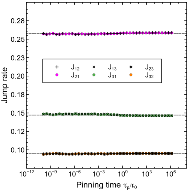
(a)    (b)

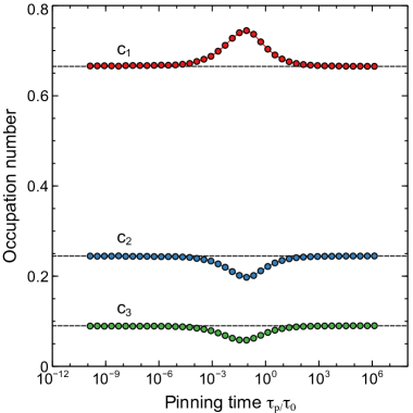
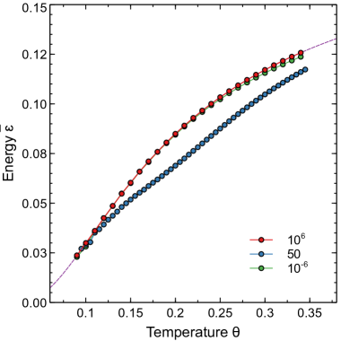
(c)   (d)

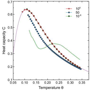
Figure 5: Results of KMC simulations for a three-level system with the pinning strength of $\alpha=1.5$. (a) Jump rates at the temperature of $\theta=0.2$ as a function of reduced pinning time $\tau_{p}/\tau_{0}$ ($\tau_{0}=74$ being the residence time at this temperature). (b) State occupation probabilities as a function of $\tau_{p}/\tau_{0}$ at $\theta=0.2$. (c) Expectation value of the system energy as a function of temperature for three values of the pinning time $\tau_{p}$ shown in the legend. (d) Heat capacity as a function of temperature for the same three pinning times. The points were computed from the fluctuation formula (34). The dashed line represents the true heat capacity $C=d\bar{\varepsilon}/d\theta$ obtained by numerical differentiation.

References

- (1) A. P. Sutton and R. W. Balluffi. Interfaces in Crystalline Materials. Clarendon Press, Oxford, (1995).
- (2) J. W. Cahn. The impurity-drag effect in grain boundary motion. Acta Metall. 10 (1962) 789–798.
- (3) K. Lücke and H. P. Stüwe. On the theory of grain boundary motion. In: L. Himmel, ed., Recovery and Recrystallization of Metals. Interscience Publishers, New York, 1963 171–210.
- (4) K. Lücke and H. P. Stüwe. On the theory of impurity controlled grain boundary motion. Acta Metall. 19 (1971) 1087–1099.
- (5) N. Ma, S. A. Dregia and Y. Wang. Solute segregation transition and drag force on grain boundaries. Acta Mater. 51 (2003) 3687–3700.
- (6) J. Li, J. Wang and G. Yang. Phase field modeling of grain boundary migration with solute drag. Acta Mater. 57 (2009) 2108–2120.
- (7) S. Shahandeh, M. Greenwood and M. Militzer. Friction pressure method for simulating solute drag and particle pinning in a multiphase-field model. Model. Simul. Mater. Sci. Eng. 20 (2012) 065008.
- (8) K. Grönhagen and J. Agren. Grain-boundary segregation and dynamic solute drag theory — A phase-field approach. Acta Mater. 55 (2007) 955–960.
- (9) F. Abdeljawad, P. Lu, N. Argibay, B. G. Clark, B. L. Boyce and S. M. Foiles. Grain boundary segregation in immiscible nanocrystalline alloys. Acta Mater. 126 (2017) 528–539.
- (10) M. Alkayyali and F. Abdeljawad. Grain boundary solute drag model in regular solution alloys. Physical Review Letters 127 (2021) 175503.
- (11) M. Greenwood, C. Sinclair and M. Militzer. Phase field crystal model of solute drag. Acta Mater. 60 (2012) 5752–5761.
- (12) M. I. Mendelev and D. J. Srolovitz. Impurity effects on grain boundary migration. Model. Simul. Mater. Sci. Eng. 10 (2002) R79–R109.
- (13) H. Sun and C. Deng. Direct quantification of solute effects on grain boundary motion by atomistic simulations. Comp. Mater. Sci. 93 (2014) 137–143.
- (14) A. T. Wicaksono, C. W. Sinclair and M. Militzer. A three-dimensional atomistic kinetic Monte Carlo study of dynamic solute-interface interaction. Model. Simul. Mater. Sci. Eng. 21 (2013) 085010.
- (15) M. I. Mendelev, D. J. Srolovitz and W. E. Grain-boundary migration in the presence of diffusing impurities: simulations and analytical models. Philos. Mag. 81 (2001) 2243–2269.
- (16) M. J. Rahman, H. S. Zurob and J. J. Hoyt. Molecular dynamics study of solute pinning effects on grain boundary migration in the aluminum magnesium alloy system. Metall. Mater. Trans. A 47 (2016) 1889–1897.
- (17) S. G. Kim and Y. B. Park. Grain boundary segregation, solute drag and abnormal grain growth. Acta Mater. 56 (2008) 3739–3753.
- (18) R. Koju and Y. Mishin. Direct atomistic modeling of solute drag by moving grain boundaries. Acta Mater. 198 (2020) 111–120.
- (19) R. K. Koju and Y. Mishin. The role of grain boundary diffusion in the solute drag effect. Nanomaterials 11 (2021) 2348.
- (20) Y. Mishin. submitte as Part II of this work.
- (21) G. H. Vineyard. Frequency factors and isotope effects in solid state rate processes. Journal of Physics and Chemistry of Solids 3 (1957) 121–127.
- (22) J. W. Cahn and F. R. N. Nabarro. Thermal activation under shear. Philosophical Magazine A 81 (2001) 1409–1426.
- (23) A. H. Cottrell. Thermally activated plastic glide. Philosophical Magazine Letters 82 (2002) 65–70.
- (24) V. A. Ivanov and Y. Mishin. Dynamics of grain boundary motion coupled to shear deformation: An analytical model and its verification by molecular dynamics. Phys. Rev. B 78 (2008) 064106.
- (25) D. Chachamovitz and D. Mordehai. The stress-dependent activation parameters for dislocation nucleation in molybdenum nanoparticles. Scientific Reports 8 (2018) 3915.
- (26) J. P. Hirth and J. Lothe. Theory of Dislocations. Wiley, New York, second edition, (1982).
- (27) A. H. Cottrell. Effect of solute atoms on behavior of dislocations. In: Report of a Conference on Strength of Solids, Lodon, UK, (1948). The Physical Society, 1948 30–38.
- (28) A. Cottrell and B. A. Bilby. Dislocation theory of yielding and strain aging of iron. Proc. Phys. Soc. London 62 (1949) 49–62.
- (29) A. H. Cottrell. Dislocations and plastic flow in crystals. Clarendon Press, Oxford, (1953).
- (30) M. K. Chari. On reversible semi-Markov processes. Operations Research Letters 15 (1994) 157–161.
- (31) S.-Z. Yu. Hidden semi-Markov models. Artificial Intelligence 174 (2010) 215–243.
- (32) H. Wang and H. Qian. On detailed balance and reversibility of semi-Markov processes and single-molecule enzyme kinetics. Journal of Mathematical Physics 48 (2007) 013303.
- (33) C. Maes, K. Netočný and B. Wynants. Dynamical fluctuations for semi-Markov processes. Journal of Physics A: Mathematical and Theoretical 42 (2009) 365002.
- (34) L. D. Landau and E. M. Lifshitz. Statistical Physics, Part I, volume 5 of Course of Theoretical Physics. Butterworth-Heinemann, Oxford, third edition, (2000).
- (35) Y. Mishin. Thermodynamic theory of equilibrium fluctuations. Annals of Physics 363 (2015) 48–97.
- (36) V. I. Manousiouthakis and M. W. Deem. Strict detailed balance is unnecessary in Monte Carlo simulation. The Journal of Chemical Physics 110 (1999) 2753–2756.
(a)
(b)
(a)  (b)
(b)
(c)  (d)
(d)
(a)  (b)
(b)
(c) (d)
(d)