A Recommender System Approach for Very Large-scale Multiobjective Optimization

Abstract

We define very large multi-objective optimization problems to be multiobjective optimization problems in which the number of decision variables is greater than 100,000 dimensions. This is an important class of problems as many real-world problems require optimizing hundreds of thousands of variables. Existing evolutionary optimization methods fall short of such requirements when dealing with problems at this very large scale. Inspired by the success of existing recommender systems to handle very large-scale items with limited historical interactions, in this paper we propose a method termed Very large-scale Multiobjective Optimization through Recommender Systems (VMORS). The idea of the proposed method is to transform the defined such very large-scale problems into a problem that can be tackled by a recommender system. In the framework, the solutions are regarded as users, and the different evolution directions are items waiting for the recommendation. We use Thompson sampling to recommend the most suitable items (evolutionary directions) for different users (solutions), in order to locate the optimal solution to a multiobjective optimization problem in a very large search space within acceptable time. We test our proposed method on different problems from 100,000 to 500,000 dimensions, and experimental results show that our method not only shows good performance but also significant improvement over existing methods.

I Introduction

Multiobjective optimization problems involve multiple conflicting objectives and have many applications in the real world [1, 2]. However, for many scientific and engineering areas, there exist a variety of multiobjective optimization problems containing a large number of decision variables, which is denoted as a large-scale multiobjective optimization problem (LSMOP) [3, 4]. A good example for the LSMOP is structure learning for deep neural networks [5], which aims at finding the optimal structure with high representation ability and better generalization, and the structure of the deep learning model always involves hundreds or even thousands of variables.

To address the curse of dimensionality, massive multiobjective evolutionary algorithms have been tailored for LSMOPs in recent years [6, 7, 8, 9, 10]. The first evolutionary algorithm for solving LSMOPs based on decision variable grouping is CCGDE3 proposed by Antonio et al. [11], which maintains multiple subgroups of equal length. Zille et al. proposed a weighted optimization framework (WOF) [12] based on grouping mechanisms, which employed a population-based algorithm as an optimizer for both original variables and weight variables. He et al. [13] designed a novel search strategy-based evolutionary multiobjective optimization algorithm driven by generative adversarial networks (GMOEA), which enhanced searching for offspring via GANs.

With the deepening of research on large-scale multiobjective optimization problems, more problems have been modeled as LSMOPs and more large-scale algorithms have been proposed. However, the existing definition of LSMOP refers to problems of more than 100 dimensions, and the corresponding algorithms are less concerned with very large-scale problems of hundreds of thousands of variables. In spite of various approaches for improving the search efficiency in LSMOPs, these methods mainly concentrate on addressing decision variables directly, which is only effective when the number of decision variables is not very large. However, when large-scale problems are encountered in industrial production, the number of variables is often more than 100,000 [14], and this is far beyond what these algorithms can handle.

Based on the aforementioned, we give a definition of very large-scale multiobjective optimization problems (VLSMOPs), characterized by involving more than 100,000 decision variables. The difficulty of VLSMOPs lies in the difficulty of locating the Pareto-optimal frontier within the limited function evaluation caused by the curse of dimensionality. Consequently, spending huge time exploring very large decision space is impractical for solving real-world problems.

In fact, a similar problem also emerges in the context of a recommender system (RS) [15, 16, 17], known as the cold-start problem [18]. The RS designed for solving such problems can effectively help the customer discover information and settle on choices from a huge amount of data with limited historical interactions. In order to locate the optimal solution in a very large search space with a reasonable number of evaluations, we introduce the idea of solving the cold start problem in RSs into solving VLSMOPs. This intuitive idea aims to recommend directions for solutions to evolve with limited historical evaluation, rather than blindly searching in a very large-scale decision space.

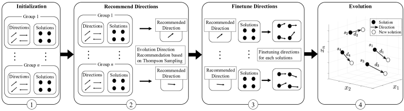
Figure 1: Illustration of the proposed method very-large-scale multiobjective optimization via recommender system (VMORS). 1. Initialize a set of directions and solutions and randomly partition them into several groups. 2. Recommend a direction for each group. 3. Fine-tune directions for all solutions based on recommended directions. 4. Evolution.

In this paper, to address problems with very large-scale decision variables, we propose a very large-scale multiobjective optimization algorithm based on a recommender system, termed VMORS. VMORS firstly transforms the optimization problem into a recommendation problem, which it then solves via Thompson sampling [19] to recommend several promising directions in the very large-scale decision space. To ensure that the algorithm can still search the decision space effectively, we design directions fine-tuning algorithm to calculate finer directions based on recommended directions. Finally, customized directions are used to evolve each solution. An illustration of the proposed framework is presented in Fig. 1. The main new contributions of this paper are as follows:

1. A method based on Recommender System is proposed to solve very large-scale multiobjective optimization problems, which is a common optimization problem in the industry.

2. We model the optimization problem as a problem in recommender systems for the first time. The proposed algorithm transforms the directed search into a recommender system problem and uses the classic Thompson sampling algorithm that solves the cold-start problem in RS. The adopted method enables the algorithm to recommend the evolution direction for locating solutions in a very large-scale search space within limited function evaluations.

3. The directions fine-tuning method optimizes the directions based on the recommended directions, which bestows solutions with the possibility to explore the whole decision space. Based on recommended directions, the directions fine-tuning method enables the algorithm to search at a fine-grained level even in a very large-scale search space.

The remainder of this paper is organized as follows. In Section II, we define VLSMOPs and present related works about LSMOPs and recommender system. The details of our novel proposed approach are presented in Section III. In Section IV, we conduct a series of experimental comparisons between our proposed method and several state-of-the-art large-scale multiobjective optimization algorithms. Finally, conclusions are drawn and future work is discussed in Section V.

II Preliminary Studies and Related Work

II-A Very large-scale Multiobjective Optimization

The mathematical form of LSMOPs is as follows:

$$\textbf{min}\ \boldsymbol{F}(\boldsymbol{x})= <f_{1}(\boldsymbol{x}),f_{2}(\boldsymbol{x}),\dots,f_{m}(\boldsymbol{x})>$$ (1)

$$\textrm{s.t.}~{}\boldsymbol{x}\in\Omega$$

where $\boldsymbol{x}=(x_{1},x_{2},...,x_{n})$ is $n$-dimensional decision vector, $\boldsymbol{F}=(f_{1},f_{2},\dots,f_{m})$ is $m$-dimensional objective vector.

Suppose $\boldsymbol{x}_{1}$ and $\boldsymbol{x}_{2}$ are two solutions of an MOP, solution $\boldsymbol{x}_{1}$ is known to Pareto dominate solution $\boldsymbol{x}_{2}$ (denoted as $\boldsymbol{x}_{1}\prec\boldsymbol{x}_{2}$), if and only if $f_{i}(\boldsymbol{x}_{1})\leqslant f_{i}(\boldsymbol{x}_{2})(\forall i=1,\dots,m)$ and there exists at least one objective $f_{j}(j\in\{1,2,\dots,m\})$ satisfying $f_{j}(\boldsymbol{x}_{1})<f_{j}(\boldsymbol{x}_{2})$. The collection of all the Pareto optimal solutions in the decision space is called the Pareto optimal set (PS), and the projection of PS in the objective space is called the Pareto optimal front (PF).

It is worth noting that traditional large-scale optimization problems consider the number of decision variables $n$ to be greater than $100$ [20]. However, the number of decision variables of many real-world problems, such as neural architecture search, critical node detection, and vehicle routing problem, easily exceed more than $100,000$, therefore, we define Very Large-Scale Multiobjective Optimization Problems (VLSMOPs), in which the $n$ is greater than $100,000$.

Larger scale MOPs have drawn some attention. For example, Tian et al. [21] proposed a method for solving Super-Large-Scale Sparse Multi-Objective Optimization. However, the designed algorithm requires that the decision variables of the problem are sparse, that is, there are a large number of 0 in the decision variables of the problem, which limits the algorithm. And the work of Li et al. [22], which explores higher dimensional MOPs, mainly focused on improving the speed for solving LSMOPs, and analyses and experiments on VLSMOPs are insufficient. VLSMOP has aroused interest in this field, but simultaneously, it is still an understudied topic.

II-B Related Works

Recently, many advances have been made in solving LSMOPs. These large-scale approaches are categorized into three categories: decision variable grouping based, decision space reduction based and novel search strategy based approaches [3].

II-B1 Decision Variable Grouping Based

The first category is based on decision variable grouping. CCGDE3, proposed by Antonio et al. [11], was the first multiobjective evolutionary algorithm for solving LSMOPs. It maintains numerous distinct subgroups and optimizes LSMOP in a divide-and-conquer manner. Afterwards, random grouping [23] and differential grouping [24] techniques were introduced to solve LSMOPs.

Another subcategory in decision variable grouping based methods is variable analysis based [25]. MOEA/DVA was presented by Ma et al. in [26] to partition the decision variables by analyzing their control property. To partition the decision variables more generically, Zhang et al. [27] proposed a large-scale evolutionary algorithm based on a decision variable clustering approach.

II-B2 Decision Space Reduction Based

The second category is based on dimensionality reduction [28]. Principal component analysis was suggested to solve LSMOPs by Liu et al. in [29], which is PCA-MOEA. Furthermore, unsupervised neural networks were used by Tian et al. to solve large-scale problems by learning the Pareto-optimal subspace [9].

In this category, problem transformation based algorithms have been suggested to solve LSMOPs. Zille et al. [12] proposed a weighted optimization framework (WOF) that was intended to serve as a generic method that can be used with any population-based metaheuristic algorithm. He et al. [30] proposed a large-scale multiobjective optimization framework as a general framework, which reformulated the original LSMOP as a low-dimensional single-objective optimization problem.

II-B3 Novel Search Strategy Based

The third category is based on the novel search strategy [31, 32]. Qin et al. [33] proposed a large-scale multiobjective evolutionary algorithm by direct sampling. Tian et al. proposed a competitive swarm optimizer based efficient search for solving LSMOPs. In addition, Hong et al. proposed a scalable algorithm with an enhanced diversification mechanism in [34]. Recently, Wang et al. [35] proposed a generative adversarial network based manifold interpolation framework to learn the manifold and generate high-quality solutions on this manifold. And Hong et al. proposed a model based on the trend prediction model and generating-filtering strategy to tackle LSMOPs.

Based on the above discussion, we can see that many algorithms have been proposed for solving LSMOPs over the years. However, the scale of experiments on these algorithms is often less than 100,000 dimensions. In Section IV, we further observe that these algorithms are less powerful to handle very large-scale problems. Therefore, we propose a new approach (VMORS) to address this problem. Compared to blindly searching in the very large-scale search space, we suggest recommending directions and then optimizing the directions for very large-scale multiobjective optimization problems.

II-C Recommender System

Recommender Systems exploit interaction history to estimate user preference and have been widely used in various industry applications[36]. Such systems are designed to estimate the utility of an item and predict whether it is worth recommending, and as such recommendation techniques fall into three broad categories: content-based, collaborative filtering based, and knowledge-based approaches[37].

II-C1 Cold-start

One challenge of Recommender Systems is to handle the situation in which users have few historical interactions. Cold-start users typically interact with the system very briefly, but still expect to receive high-quality recommendations [38]. A natural way to tackle this is through the idea of the Exploration-Exploitation trade-off. For exploitation, the system takes advantage of the best option that is known, and for exploration, the system takes some risks to collect information about unknown options. Such a trade-off is also a very important topic in multiobjective optimization problems.

II-C2 Thompson sampling

Thompson sampling (TS) [39] is a commonly used bandit strategy in recommender systems. Thompson sampling was first proposed in 1933 [40, 41] for allocating experimental effort in two-armed bandit problems arising in clinical trials. Thompson sampling strikes a balance between statistical efficiency and algorithmic complexity [19], and is widely adopted in Recommender Systems [38]. Later, Sun et al. [42] proposed a new adaptive operator selection mechanism for multiobjective evolutionary algorithms based on dynamic Thompson sampling.

Inspired by the success of Thompson sampling in solving cold-start problems for Recommender Systems, we transform the VLSMOP as a recommender system problem and adopt Thompson sampling for recommending directions and guiding the population to evolve. Modeling VLSMOPs as a recommender system allows the algorithm to recommend directions for solutions even in a very large-scale decision space. The use of the Thompson sampling method allows the algorithm to avoid searching directly in high-dimensional decision space while recommending directions while accommodating both statistical and computational efficiency [19].

III Very large-scale Multiobjective Optimization via Thompson sampling

III-A Overview

To effectively search in very large-scale decision space, the VLSMOP is transformed into the cold-start problem and Thompson sampling is adopted to solve this problem. The transformation regards the solution as the user and the direction as the item. The aim is to recommend directions that can guide evolution in a very large-scale search space under limited computational resources, and make reasonable use of these recommended directions to optimize directions.

Each iteration of the proposed framework can be divided into evolution directions recommendation, evolution directions fine-tuning, and population evolution. Specifically, in the first step, Thompson sampling is adopted to learn and recommend best directions. Second, a more refined directions fine-tuning based on recommended direction is suggested. Thirdly, the fine-tuned directions are used to guide the population to evolve toward the Pareto-optimal front.

III-B Evolution Directions Recommendation based on Thompson sampling

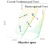
(a)

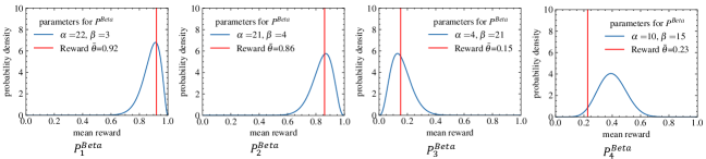
(b)

Figure 2: Illustration of Thompson sampling on the direction. Firstly, each individual has one direction ($\boldsymbol{d}_{i}$) in the decision space, and each direction guide the individual to evolve once. Secondly, each individual ($\boldsymbol{p}_{i}$) is evolved and evaluated in objective space. According to the evaluation result, algorithm updates corresponding $\alpha$ and $\beta$ parameters for each directions. ($\alpha$ and $\beta$ in each direction are the number of times the individual evolved and the number of times the individual $\boldsymbol{p}_{i}$ degenerated along the direction $\boldsymbol{d}_{i}$). Thirdly algorithm calculates the $P^{Beta}(\theta)$ distribution in each direction (blue lines in $P^{Beta}_{i}$, and samples the mean reward $\bar{\theta}_{i}$ on the $P^{Beta}(\theta)$ distribution (the red lines in $P^{Beta}_{i}$). Then select the direction corresponding to the distribution with the highest mean reward $\bar{\theta}_{i}$. The direction sampled of this example is the direction $\boldsymbol{d}_{1}$ according to $P^{Beta}_{1}$.

For solutions $\mathcal{S}=\{\boldsymbol{s}_{i}\}$ with dimension $d$, it is impossible to locating directions $\mathcal{D}=\{\boldsymbol{d}_{j}\}$ toward the PS in the whole search space since it is very large scale. Therefore, we transform the direction optimization into a cold-start problem and apply Thompson sampling to recommend the best directions.

The evolution direction for a solution is defined as $\boldsymbol{d}~{}(\boldsymbol{d}=(d_{1},d_{2},\dots,d_{d}))$. The algorithm will recommend directions for solutions and then fine-tuning directions for each solutions.

The cold-start problem considers allocating a fixed set of limited resources among large-scale items $\mathcal{I}=\{i_{1},\dots,i_{k}\}$ that maximizes the expected return for users $\mathcal{U}=\{u_{1},\dots,u_{l}\}$. In the proposed framework, each solution $\boldsymbol{s}_{i}$ is regarded as a user $u_{i}$, an item $i_{j}$ is the direction $\boldsymbol{d}_{j}$ to guide the evolution of the solution. The response of user $u_{i}$ to the item $i_{j}$, or denoted as the reward $r_{ij}$ is the quality of solution $\boldsymbol{s}_{i}$ after evolving along the direction $\boldsymbol{d}_{j}$. The ultimate goal of this RS is to recommend the best directions with limited computation for solutions to evolve toward the Pareto-optimal front.

Input: $\boldsymbol{\alpha}$(Set of parameters $\alpha$), $\boldsymbol{\beta}$(Set of parameters $\beta$), $\mathcal{F}$ (the non-dominated set)).

1 for $\boldsymbol{f}_{i}$ in $\mathcal{F}$ do

2       if $f_{i}=1$ then $r_{i}\leftarrow 1$ ;

3       else $r_{i}\leftarrow 0$ ;

4       $\alpha_{i}\leftarrow\alpha_{i}+r_{i}$;

5       $\beta_{i}\leftarrow\beta_{i}+1-r_{i}$ ;

6      

7 end for

Algorithm 1 Parameter Update

Thompson sampling is an efficient algorithm for solving the cold-start problem. In Thompson sampling, each item is assigned an independent prior reward distribution of $\theta_{j},j\in\{1,\dots,k\}$. In particular, a Beta distribution with parameters $\alpha=(\alpha_{1},\dots,\alpha_{k})$ and $\beta=(\beta_{1},\dots,\beta_{k})$ is used to represent this prior distribution:

$$P^{Beta}(\theta_{j})=\frac{\Gamma(\alpha_{j}+\beta_{j})}{\Gamma(\alpha_{j})\Gamma(\beta_{j})}\theta_{j}^{\alpha_{j}-1}(1-\theta_{j})^{\beta_{j}-1}$$ (2)

where $\alpha_{j}$ and $\beta_{j}$ are the parameters associated with the $j$-th item $i_{j}$, and $\Gamma(\cdot)$ is the gamma function. For a given item $i_{j}$ for user $u_{i}$, if its reward for user $u_{i}$ is $r_{ij}=1$, then $\alpha_{j}$ and $\beta_{j}$ are updated as:

$$\alpha_{j}=\alpha_{j}+1,\beta_{j}=\beta_{j}.$$ (3)

Otherwise, if $r_{ij}=0$ then we have:

$$\alpha_{j}=\alpha_{j},\beta_{j}=\beta_{j}+1.$$ (4)

In our method, the Thompson sampling algorithm is adopted to recommend best directions. The item $i_{j}$ is the direction $\boldsymbol{d}_{j}$. Then, the reward $r_{ij}$ of the direction $d_{j}$ is the quality of the solution $\boldsymbol{s}_{i}$ after applying the evolution algorithm with the direction of $\boldsymbol{d}_{j}$, and the dominance of the solution is adopted to evaluate the quality of the solution:

$$r_{ij}=\begin{cases}1,&\text{New solution evolved by\ }\boldsymbol{d}_{j}\text{\ Pareto-dominates\ }\boldsymbol{s}_{i}\\ 0,&\text{Otherwise}\end{cases}$$ (5)

Since an evolutionary algorithm is adopted when evolving directions, the fixed reward distribution in Eq. (2) does not fit the non-stationary nature of the possible solutions. To address this problem, in our specific implementation, a dynamic Thompson sampling [43] strategy is adopted, which is presented in Algorithm 1. $\alpha$ and $\beta$ of each distribution are initialized to be 1, and $P^{Beta}(\theta_{i})$ is initialized to be a uniform distribution over $[0,1]$.

Input: $\mathcal{D}=\{\boldsymbol{d}\}$ (A set of directions), $\mathcal{S}=\{s_{i}\}$(A set of solutions), $n_{d}$ (Number of recommended directions), $e$ (Function evaluation for Thompson sampling).

Output: $\mathcal{\hat{D}}=\{\boldsymbol{d}\}$ (A set of sampled directions), $\{\mathcal{S}_{i}\}$ (Grouped solutions).

1 $\mathcal{\hat{D}}\leftarrow\emptyset$, $\mathcal{\hat{S}}\leftarrow\emptyset$ ;

2 $\{\mathcal{D}_{i}\}\leftarrow$ Divide the set $\mathcal{D}$ into $n_{d}$ groups randomly;

3 $\{\mathcal{S}_{i}\}\leftarrow$ Divide the set $\mathcal{S}$ into $n_{d}$ groups randomly;

4

5for $\mathcal{D}_{i}$ in $\{\mathcal{D}_{i}\}$ and $\mathcal{S}_{i}$ in $\{\mathcal{S}_{i}\}$ do

6       $n\leftarrow$ size of $\mathcal{D}_{i}$ ;

7       $\boldsymbol{\alpha}\leftarrow\boldsymbol{1}\in\mathbb{R}^{n\times 1}$; $\boldsymbol{\beta}\leftarrow\boldsymbol{1}\in\mathbb{R}^{n\times 1}$;

8       while $e$ is not exhausted do

9             for $d_{j}\in\mathcal{D}_{i}$ and $\boldsymbol{s}_{j}\in\mathcal{S}_{d}$ do

10                   $\boldsymbol{s}_{j}=\boldsymbol{s}_{j}+\boldsymbol{d}_{j}$;

11                  

12             end for

13            $\mathcal{F}\leftarrow$ Fast-Non-Dominated-Sort($\mathcal{S}_{i}$) ;

14             Parameter-Update$(\boldsymbol{\alpha},\boldsymbol{\beta},\mathcal{F})$ ;

15             Use evolutionary algorithm on $S_{i}$ with evaluation of $\mathcal{F}$ to obtain new set of $S_{i}$ ;

16            

17       end while

18      for $i\leftarrow 1$ to $n$ do

19             Sample the estimated mean reward $\bar{\theta}_{i}$ from Beta distribution $P^{Beta}(\alpha_{i},\beta_{i})$ ;

20            

21       end for

22      $k\leftarrow\arg\max_{i\in\{1,\dots,n\}}\bar{\theta}_{i}$ ;

23       $\mathcal{\hat{D}}\leftarrow\mathcal{\hat{D}}\cup\{\boldsymbol{d}_{k}\}$;

24      

25 end for

Algorithm 2 Evolution Direction Recommendation based on Thompson sampling

The Thompson sampling algorithm recommends the direction $\boldsymbol{d}$. The reward $r_{ij}$ of using direction $\boldsymbol{d}_{j}$ by for solution $\boldsymbol{s}_{i}$ is calculated by evaluating the new solution $\boldsymbol{\hat{s}}_{i}$ evolved with $\boldsymbol{d}_{j}$. For each group of solutions $\mathcal{S}_{i}$, we will recommend a best direction $\boldsymbol{d}_{k}$ from the group of directions $\mathcal{D}_{i}$. The algorithm for sampling directions is described in Algorithm 2, and an illustrative example of Thompson sampling on the direction method is given in Fig. 2.

III-C Evolution Directions Fine-tuning

To search in a very large-scale decision space, a key problem that needs to be solved is the sufficiency of evolution directions. Direction recommendation based on Thompson sampling provides us with a small number of potential evolutionary directions. To address the insufficiency of evolutionary directions, we propose the method of fine-tuning directions for each solution in this section.

The essence of fine-tuning directions is to fine-tune the potential directions obtained by the recommendation, so as to generate a unique and suitable evolutionary direction for each solution.

For paired group of solutions $\mathcal{S}_{i}$ and group of directions $\mathcal{D}_{d}$, we have recommended direction $\boldsymbol{d}_{k}$. To achieve to purpose of fine-tuning for each solution, we generate direction population based on the recommended direction $\boldsymbol{d}_{k}$ and select a set of representative solutions from the group of solutions $\mathcal{S}_{i}$ to evaluate the corresponding population.

Figure 3: Illustration of directions fine-tuning. 1. For paired group of solutions $\mathcal{S}_{i}$ and group of directions $\mathcal{D}_{d}$. 2. Initialize a set of direction populations based on the recommended direction, then evolve each solution with direction population and evaluating; 4. Obtain a set of directions for each solution.

The algorithm selects representative solution with the largest crowding distance on the first non-dominated front from grouped solutions $\mathcal{S}_{i}$. For each representative solution $\boldsymbol{s}_{d}$, the algorithm firstly initializes a set of random direction population $\mathcal{D}_{p}=\{\boldsymbol{d}_{i}+\boldsymbol{d}_{k}\}$ based on recommended directions $\boldsymbol{d}_{k}$, the size of $\mathcal{D}_{p}$ is $n_{di}=N/n_{d}$. Second, solution $\boldsymbol{s}_{d}$ will be evolved with direction population and evaluated. Afterwards, we apply an evolutionary algorithm on the direction population and repeat.

We perform the evolution directions fine-tuning method on each grouped solution $\mathcal{S}_{i}$ and recommended direction $\boldsymbol{d}_{k}$. Finally, we obtain a set of directions for each solution based on the recommended direction. The visualization of directions fine-tuning is presented in Fig. 3 and the process is given in Algorithm 3.

Input: $\mathcal{D}=\{\boldsymbol{d}_{k}\}$ (Evolution directions recommended), $\{\mathcal{S}_{i}\}(\mathcal{S}_{i}=\{\boldsymbol{s}_{i}\}$)(A set of grouped solutions), $e$ (Function evaluation for Evolution Directions Fine-tuning).

Output: $\mathcal{D}=\{\boldsymbol{v}_{i}\}$ (A set of directions), $\mathcal{S}$ (Solutions produced during directions fine-tuning).

1 $N\leftarrow$ size of $\mathcal{S}$;

2 $n_{d}\leftarrow$ size of $\mathcal{D}$ ;

3 $n_{di}\leftarrow N/n_{d}$ // Size for Direction Population ;

4 $\mathcal{V}\leftarrow\emptyset$ ;

5 for $\boldsymbol{d}_{k}\in\mathcal{D}$ and $\mathcal{S}_{i}$ in $\{\mathcal{S}_{i}\}$ do

6       $\boldsymbol{s}_{d}\leftarrow$ Select diversity solutions $(\mathcal{S}_{i},n_{di})$ ;

7       $\mathcal{D}_{p}\leftarrow$ Initialize direction population with size $n_{di}$ based on recommended direction $\boldsymbol{d}_{k}$;

8       while $e$ is not exhausted do

9             for $\boldsymbol{d}_{i}\in\mathcal{D}_{p}$ do

10                   $\boldsymbol{s}_{i}\leftarrow\boldsymbol{s}_{d}+\boldsymbol{d}_{i}$ ;

11                   $\mathcal{S}_{p}\leftarrow\mathcal{S}_{p}\cup\{\boldsymbol{s}_{i}\}$;

12                  

13             end for

14            $\mathcal{F}\leftarrow$ Fast-Non-Dominated-Sort($\mathcal{S}_{p}$) ;

15             Use evolutionary algorithm on $\mathcal{D}_{p}$ with evaluation of $\mathcal{F}$ to obtain a new set of $\mathcal{D}_{p}$ ;

16            

17       end while

18      for $i\leftarrow 1$ to $n_{di}$ do

19             $\mathcal{V}\leftarrow\mathcal{V}\cup\{\boldsymbol{v}_{i}\}$;

20             $\mathcal{S}\leftarrow\mathcal{S}\cup\mathcal{S}_{p}$;

21            

22       end for

23      

24 end for

Algorithm 3 Evolution Directions Fine-tuning

III-D A Recommender System Approach for Very Large-scale Multiobjective Optimization

The whole framework of the algorithm is presented in Algorithm 4. In this algorithm, we use a particle swarm algorithm in the optimization step. The algorithm uses the set of directions $\mathcal{D}$ as the initial directions of the particle swarm. After particle swarm optimization, the direction of each solution is recorded as the initial direction for the next iteration of recommending direction.

Input: $N$ (population size), $n_{d}$ (sampled directions size), $e$ (Function evaluation for recommending, fine-tuning and evolving.)

1 $\mathcal{S}\leftarrow$ Initialize a set of solutions with size $N$ ;

2 $\mathcal{D}\leftarrow$ Initialize a set of directions with size of $N$ ;

3 while termination criterion is not fulfilled do

4       $(\mathcal{\hat{D}},\mathcal{S})\leftarrow$ Evolution Direction Recommendation based on Thompson sampling $(\mathcal{D},\mathcal{S},n_{d},e)$ ;

5       $(\mathcal{D},\mathcal{S})\leftarrow$ Evolution Directions Fine-tuning $(\mathcal{\hat{D}},\mathcal{S},e)$ ;

6       $(\mathcal{D},\mathcal{S})\leftarrow$ Optimization Algorithm $(\mathcal{D},\mathcal{S},e)$ ;

7      

8 end while

Algorithm 4 VMORS

IV Experimental Studies

IV-A Algorithms Used in Comparison and Test Problems

In this section, several experiments are conducted to empirically investigate the performance of our proposed algorithm VMORS. The proposed VMORS is compared with several state-of-the-art MOEAs, including NSGA-II[1], CCGDE3 [11], WOF [12], LSMOF[30], LMOCSO[20], GMOEA [44] and DGEA [32]. All the compared algorithms are implemented on PlatEMO [45]. NSGA-II, as the baseline, is an MOEA for solving multiobjective optimization problems. CCGDE3 is a typical method for solving the LSMOP by decision variable grouping. WOF and LSMOF are two representative frameworks based on decision space reduction. LMOCSO and GMOEA are two promising methods based on novel search strategy, and they used competitive swarm optimizer and generative adversarial network, respectively. DGEA is a method that also used ideas like sampling and direction vectors but is completely different from our approach. DGEA selected a balanced parent population and used them to construct direction vectors in the decision spaces for reproducing promising offspring solutions.

The benchmark LSMOP [46] are widely used for comparing the performance of large-scale MOEAs. LSMOP1 – LSMOP4 have a linear Pareto front, LSMOP5 – LSMOP8 have a convex Pareto front, and LSMOP9 has a disconnected Pareto front. LSMOP1 and LSMOP5 have a unimodal fitness landscape, and for LSMOP3 and LSMOP7, their modality is multi-modal, and others are mixed. We also included TREE [14] in the experiments as a real-world problem. The problem has dimensions up to 900,000, which constitutes VLSMOPs.

In the experiments, the IGD [47] and HV [48] metric is utilized to evaluate the convergence and the diversity of compared algorithms. For testing the statistical significance of the differences between metric values, each algorithm is run 20 times independently, and we use the Wilcoxon rank-sum test [49] to compare the statistic results, we report a difference at a significance level of 0.05. Symbols ”+”, ”-” and ”=” indicate the algorithm is significantly better than, significantly worse than, and statistically tied by our proposed VMORS.

IV-B Parameter Settings

TABLE I: The Time of State-Of-The-Art Large-scale MOEAs and Our Proposed Method for Solving 1000-Dimensional Bi-objective LSMOP 1. (100,000FEs, unit: s)

CCGDE3	MOEA/DVA	LMEA	WOF	LSMOF
16.61	1709	1582	34.26	27.58
MOEA/PSL	LMOCSO	GMOEA	DGEA	VMORS
4993	28.15	2569	28.27	25.52

IV-B1 Decision Variables

In VLSMOPs, the number of decision variables are 100,000, 500,000 and 1,000,000, and 100 to 20,000 for LSMOPs.

TABLE II: IGD Metric Obtained by Compared Algorithms Over Bi-Objective VMOP Problems with Dimension 1,000,000. The Best Result in Each Row is Highlighted in Bold.

Problem	D	NSGA-II	CCGDE3	MOEA/DVA	WOF	LSMOF	LMOCSO	GMOEA	DGEA	VMORS	ROC(%)
LSMOP1	1,000,000	1.17e+01-	6.39e+00-	-	3.11e-01-	3.48e-01-	1.80e+00-	-	3.34e-01-	1.59e-01	48.83%
LSMOP2	1,000,000	4.97e-03=	5.00e-03=	-	3.72e-03=	4.54e-03=	3.82e-03=	-	3.59e-03=	4.30E-03	-19.91%
LSMOP3	1,000,000	3.96e+01-	3.42e+01-	-	Inf-	1.58e+00=	2.20e+03-	-	1.36e+01-	1.57e+00	0.39%
LSMOP4	1,000,000	7.41e-03=	7.04e-03=	-	3.73e-03=	4.55e-03=	5.32e-03=	-	3.61e-03=	4.41E-03	-22.23%
LSMOP5	1,000,000	2.50e+01-	1.40e+01-	-	7.42e-01-	7.42e-01-	3.70e+00-	-	7.46e-01-	6.84e-01	7.85%
LSMOP6	1,000,000	7.42e-01-	7.42e-01-	-	3.69e-01-	3.06e-01-	1.12e+03-	-	7.42e-01-	1.48e-01	51.66%
LSMOP7	1,000,000	9.21e+04-	3.74e+04-	-	1.52e+00=	1.52e+00=	2.29e+03-	-	1.52e+00=	1.52e+00	0.01%
LSMOP8	1,000,000	2.08e+01-	1.19e+01-	-	2.93e-01-	7.42e-01-	3.21e+00-	-	7.02e-01-	1.55e-01	46.99%
LSMOP9	1,000,000	6.07e+01-	3.05e+01-	-	Inf-	8.02e-01-	1.68e+01-	-	2.19e+01-	5.24e-01	34.71%
(+/-/=)		0/7/2	0/7/2	0/9/0	0/6/3	0/5/4	0/7/2	0/9/0	0/6/3

TABLE III: HV Metric Obtained by Compared Algorithms Over Tri-Objective LSMOP Problems with Dimension 1,000,000. The Best Result in Each Row is Highlighted in Bold.

Problem	D	NSGAII	CCGDE3	MOEADVA	WOF	LSMOF	LMOCSO	GMOEA	DGEA	VMORS	ROC
LSMOP1	1000000	0.00e+00-	0.00e+00-	-	2.49e-01-	2.29e-01-	0.00e+00-	-	2.34e-01-	4.04e-01	48.83%
LSMOP2	1000000	5.80e-01=	5.80e-01=	-	5.82e-01=	5.81e-01=	5.82e-01=	-	5.82e-01=	5.82E-01	-19.91%
LSMOP3	1000000	0.00e+00=	0.00e+00=	-	0.00e+00=	0.00e+00=	0.00e+00=	-	0.00e+00=	0.00e+00	0.00%
LSMOP4	1000000	5.76e-01=	5.76e-01=	-	5.82e-01=	5.81e-01=	5.79e-01=	-	5.82e-01=	5.81E-01	-22.23%
LSMOP5	1000000	0.00e+00-	0.00e+00-	-	9.09e-02=	9.09e-02=	0.00e+00-	-	8.13e-02=	9.09e-02	7.85%
LSMOP6	1000000	9.08e-02-	9.08e-02-	-	9.62e-02-	1.08e-01-	0.00e+00-	-	9.09e-02-	1.68e-01	51.66%
LSMOP7	1000000	0.00e+00=	0.00e+00=	-	0.00e+00=	0.00e+00=	0.00e+00=	-	0.00e+00=	0.00e+00	0.00%
LSMOP8	1000000	0.00e+00-	0.00e+00-	-	1.19e-01-	9.09e-02-	0.00e+00-	-	4.91e-03-	2.11e-01	46.99%
LSMOP9	1000000	0.00e+00-	0.00e+00-	-	0.00e+00-	9.19e-02-	0.00e+00-	-	0.00e+00-	1.51e-01	34.71%
(+/-/=)		0/7/2	0/7/2	0/9/0	0/6/3	0/5/4	0/7/2	0/9/0	0/6/3

IV-B2 Population Size

Following the setting of population size for bi-objective and tri-objective problems in WOF [12], LSMOF[30] and DGEA [32], the population size $N$ is set to 100 for test benchmarks with two objectives and 105 for test benchmarks with three objectives.

IV-B3 Parameter Settings for Algorithms

According to [45], the parameters of compared algorithms are set according to their original publications. The specific parameters of each algorithm are given in Table S-1 of the supplementary material. For the proposed algorithm, the sampled directions size $n_{d}$ is set to $N/4=25$. The function evaluation $e$ for directions recommendation, directions fine-tuning and optimization algorithm are all set to $0.05E$.

IV-B4 Termination Condition

The number of maximum evaluations $E$ is set to 100,000. The number of function evaluations maybe small, but it is practical for real-world applications [30]. This is attributed to the fact that the number of function evaluations is always limited by the economic and/or computational cost, especially for the very-large-scale optimization problems.

If the algorithm requires massive time to solve VLSMOP or LSMOP, then the function evaluation is not a fair termination condition. We presented the time used for solving 1,000-dimensional LSMOP1 in Table I. Algorithms that took more than 1,000s (five times longer than general methods) are marked in bold, and we only select MOEA/DVA and GMOEA as two representatives for comparison.

TABLE IV: IGD Metric Obtained by Compared Algorithms Over Tri-Objective LSMOP Problems with Dimension 100,000, and 500,000. The Best Result in Each Row is Highlighted in Bold.

Problem	D	NSGA-II	CCGDE3	MOEA/DVA	WOF	LSMOF	LMOCSO	GMOEA	DGEA	VMORS	ROC (%)
LSMOP1	100,000	1.28e+01-	1.07e+01-	-	4.37e-01-	7.49e-01-	1.67e+00-	-	4.33e-01-	2.00e-01	53.81%
	500,000	1.55e+01-	1.36e+01-	-	4.83e-01-	1.10e+00-	2.43e+00-	-	9.20e-01-	1.82e-01	62.32%
LSMOP2	100,000	6.22e-02=	4.98e-02=	-	3.82e-02=	4.99e-02=	3.88e-02=	-	3.85e-02=	5.02E-02	-31.41%
	500,000	8.89e-02=	7.60e-02=	-	5.83e-02=	7.51e-02=	5.88e-02=	-	5.80e-02=	5.05e-02	12.93%
LSMOP3	100,000	3.88e+01-	1.84e+01-	-	8.61e-01=	8.61e-01=	3.90e+01-	-	8.62e-01=	8.61e-01	0.00%
	500,000	3.31e+01-	2.90e+01-	-	1.29e+00-	1.29e+00-	2.55e+01-	-	1.29e+00-	8.61e-01	33.26%
LSMOP4	100,000	5.62e-02=	5.99e-02=	-	5.82e-02=	5.24e-02=	5.83e-02=	-	5.82e-02=	3.30e-02	37.02%
	500,000	8.33e-02=	7.85e-02=	-	6.17e-02=	7.85e-02=	6.20e-02=	-	6.04e-02=	5.72e-02	5.30%
LSMOP5	100,000	2.13e+01-	1.71e+01-	-	5.89e-01=	9.46e-01-	3.44e+00-	-	5.57e-01-	5.01e-01	10.05%
	500,000	3.13e+01-	2.52e+01-	-	6.71e-01-	1.42e+00-	5.34e+00-	-	2.73e+00-	3.60e-01	46.35%
LSMOP6	100,000	6.75e+04-	4.88e+04-	-	1.71e+00-	7.81e-01-	1.39e+03-	-	5.07e+02-	7.05e-01	9.73%
	500,000	5.75e+04-	2.98e+04-	-	1.34e+00-	8.47e-01-	4.44e+02-	-	8.36e-01-	7.05e-01	15.67%
LSMOP7	100,000	9.47e-01-	9.47e-01-	-	4.57e-01+	9.13e-01-	9.47e-01-	-	9.13e-01-	8.34E-01	-82.49%
	500,000	9.46e-01-	9.46e-01-	-	6.69e-01-	9.13e-01-	9.46e-01-	-	1.32e+00-	6.33e-01	5.38%
LSMOP8	100,000	9.49e-01-	9.49e-01-	-	1.73e-01-	2.32e-01-	9.48e-01-	-	9.46e-01-	8.01e-02	53.70%
	500,000	9.49e-01-	9.49e-01-	-	9.75e-02=	2.16e-01-	9.49e-01-	-	1.35e+00-	7.46e-02	23.49%
LSMOP9	100,000	1.24e+02-	9.05e+01-	-	1.15e+00-	1.49e+00-	6.88e+01-	-	6.17e+01-	5.87e-01	48.96%
	500,000	1.44e+02-	8.92e+01-	-	1.27e+00-	1.14e+00-	6.63e+01-	-	6.89e+01-	5.86e-01	48.60%
(+/-/=)		0/14/4	0/14/4	0/18/0	1/10/7	0/13/5	0/14/4	0/18/0	0/13/5

TABLE V: HV Metric Obtained by Compared Algorithms Over Tri-Objective LSMOP Problems with Dimension 100,000, and 500,000. The Best Result in Each Row is Highlighted in Bold.

Problem	D	NSGA-II	CCGDE3	MOEA/DVA	WOF	LSMOF	LMOCSO	GMOEA	DGEA	VMORS	ROC (%)
LSMOP1	100,000	0.00e+00-	0.00e+00-	-	2.73e-01-	9.09e-02-	0.00e+00-	-	3.07e-01-	5.83e-01	89.90%
	500,000	0.00e+00-	0.00e+00-	-	3.97e-01-	9.09e-02-	0.00e+00-	-	1.84e-01-	6.26e-01	57.68%
LSMOP2	100,000	8.21e-01=	8.28e-01=	-	8.43e-01=	8.26e-01=	8.41e-01=	-	8.42e-01=	8.26E-01	-2.02%
	500,000	8.18e-01=	8.20e-01=	-	8.40e-01=	8.30e-01=	8.40e-01=	-	8.41e-01=	8.27E-01	-1.66%
LSMOP3	100,000	0.00e+00-	0.00e+00-	-	9.09e-02=	9.09e-02=	0.00e+00-	-	8.98e-02=	9.09e-02	0.00%
	500,000	0.00e+00-	0.00e+00-	-	9.09e-02=	9.09e-02=	0.00e+00-	-	9.09e-02=	9.09e-02	0.00%
LSMOP4	100,000	8.20e-01=	8.30e-01=	-	8.43e-01=	8.31e-01=	8.43e-01=	-	8.43e-01=	8.26E-01	-2.02%
	500,000	8.11e-01=	8.20e-01=	-	8.35e-01=	8.24e-01=	8.35e-01=	-	8.37e-01=	8.17E-01	-2.39%
LSMOP5	100,000	0.00e+00-	0.00e+00-	-	3.36e-01=	9.09e-02-	0.00e+00-	-	2.49e-01-	3.44e-01	2.38%
	500,000	0.00e+00-	0.00e+00-	-	3.40e-01=	9.09e-02-	0.00e+00-	-	0.00e+00-	3.44e-01	1.18%
LSMOP6	100,000	0.00e+00=	0.00e+00=	-	0.00e+00=	1.20e-02=	0.00e+00=	-	0.00e+00=	0.00E+00	-100.00%
	500,000	0.00e+00-	0.00e+00-	-	0.00e+00-	3.12e-03-	0.00e+00-	-	7.00e-03-	1.18e-01	1585.71%
LSMOP7	100,000	8.85e-02=	8.86e-02=	-	1.58e-01+	8.93e-02=	8.88e-02=	-	9.01e-02=	9.01E-02	-42.97%
	500,000	9.04e-02=	9.04e-02=	-	9.08e-02=	9.05e-02=	9.05e-02=	-	8.14e-02=	9.07E-02	-0.11%
LSMOP8	100,000	8.44e-02-	8.50e-02-	-	4.12e-01-	3.83e-01-	8.68e-02-	-	9.04e-02-	4.95e-01	20.15%
	500,000	8.44e-02-	8.53e-02-	-	4.60e-01=	4.00e-01-	8.58e-02-	-	8.90e-02-	5.00e-01	8.70%
LSMOP9	100,000	0.00e+00-	0.00e+00-	-	1.47e-01=	9.59e-02-	0.00e+00-	-	0.00e+00-	1.92e-01	30.61%
	500,000	0.00e+00-	0.00e+00-	-	1.29e-01-	1.48e-01=	0.00e+00-	-	0.00e+00-	1.92e-01	29.73%
(+/-/=)		0/11/7	0/11/7	0/18/0	1/5/12	0/8/10	0/11/7	0/18/0	0/9/9

IV-C Performance on VLSMOPs

In order to test the performance of our proposed algorithm for solving very-large scale multiobjective optimization problems, we set the decision variables to 1,000,000, and present the IGD values and HV values in Tables II and III. We then present the results of IGD and HV with 100,000 and 500,000 decision variables in Table IV and Table V, respectively. In the last column of each Table, we present the indicator of the rate of change (ROC) between our algorithm and the best results among other algorithms.

Generally, the proposed method has a 40% improvement compared to the suboptimal algorithm with respect to the IGD indicator. Especially in the LSMOP 8 and LSMOP 9 problems. Combined with the characteristics of these two problems, we believe that when the number of decision variables are further extended to 100,000 or more, the characteristics of the Pareto front are more complicated, and the VLSMOP with a mixed fitness landscape is especially complex. However, our algorithm can recommend the optimal direction within a reasonable number of function evaluations in such very large-scale search space, which is of great practical significance for solving such problems.

From Table II, it can be observed that our algorithm achieves significant improvement for solving 1,000,000 dimensional VLSMOPs. In LSMOP2 and LSMOP4, the IGD values of our algorithm are slightly lower, but there is no significant difference with the optimal results.

NSGA-II is a classic algorithm, but this algorithm is less effective when dealing with very-large-scale search spaces. WOF only has slightly better performance than VMORS on tri-objective LSMOP7. DGEA and LSMOF are able to handle large-scale multiobjective optimization problems, but the overall results are still poor compared to our proposed algorithm. Although LMOCSO is an effective particle swarm algorithm that can solve LSMOPs, compared to recommending directions for the population to evolve, search results without the recommender system of LMOCSO are still not good.

To verify the performance of our algorithm on real problems, we test it on the TREE dataset, and the experimental results are shown in Table VI. It can be seen from that the proposed algorithm still has a significant advantage in solving a real-world VLSMOP.

TABLE VI: IGD Metric Obtained by Compared Algorithms Over TREE problems. The Best Result in Each Row is Highlighted in Bold. Results that took more than 50,000s are represented by ’-’.

Problem	D	NSGA-II	CCGDE3	MOEA/DVA	WOF	LSMOF	LMOCSO	DGEA	GMOEA	VMORS	ROC
TREE1	100,000	-	-	-	9.71e+02-	9.55e+02-	-	9.62e+02-	-	9.53E+02	0.20%
TREE2	360,000	-	-	-	4.39e+03-	4.39e+03-	-	4.40e+03-	-	4.36E+03	0.80%
TREE3	96,000	-	-	-	9.60e+02-	8.72e+02-	-	9.60e+02-	-	5.08E+02	41.70%
TREE4	120,000	-	-	-	1.20e+03-	1.20e+03-	-	1.20e+03-	-	1.05E+03	12.81%
TREE5	900,000	-	-	-	9.28e+03-	8.90e+03-	-	9.20e+03-	-	8.16E+03	9.06%
TREE6	192,000	-	-	-	-	-	-	-	-	-	-
(+/-/=)		0/5/1	0/5/1	0/5/1	0/5/1	0/5/1	0/5/1	0/5/1	0/5/1

IV-D Performance on LSMOPs

In this section, we validate the performance of the proposed framework on LSMOPs. We conduct the experiments on bi-objective and tri-objective LSMOPs with 100, 200, 500, 1,000, 2,000, 5,000, 10,000, and 20,000 decision variables. We present the IGD values and HV values obtained by algorithms in Tables S-II to S-IX of the supplementary material.

Generally, VMORS has outperformed the eight current state-of-the-art algorithms. For example, our proposed VMORS achieves 19 best results out of 36 test instances with the decision variables from 100 too 1,000 (Table S-II of the supplementary material). VMORS obtains significant advantages over LSMOP2, LSMOP5, LSMOP6, and LSMOP8. When the dimension extends to 20,000, our algorithm is still significantly superior to all the compared algorithms. Whilst competitive in lower dimensions (from 100 to 1,000), our algorithm also has advantages in the higher dimensions. In Table S-VI of the supplementary, our proposed VMORS achieves 21 best results out of 36 bi-objective LSMOP test instances. Only WOF has two significantly better results compared to our proposed method, while the other algorithms have the best results but are not statistically better under the Wilcoxon rank-sum test.

Comparing dimensions 100 to 1,000 and 5,000 to 20,000, the performance of WOF, LMOCSO, and DGEA all decrease. WOF has more results that are significantly worse than VMORS (12 to 16), and LMOCSO and DGEA have fewer better results. However, our proposed method VMORS has more best results (19 to 21). As the number of decision variables increases, the number of best results obtained by our algorithm increases, and the same pattern can also be found in solving tri-objective LSMOPs (Please refer to the supplementary material).

Our proposed method VMORS also has better results on the HV metric for LSMOPs. Specifically, our proposed method obtained 16 and 19 best results in bi-objective and tri-objective optimization problems(Tables S-IV and S-V), respectively. In summary, our algorithm also achieves good results in terms of convergence and diversity for solving LSMOPs. Thus, we surmise that recommending directions for solutions is effective in both solving large-scale and very-large-scale multiobjective optimization problems.

IV-E Convergence Analysis

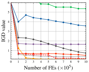
(a) 1,000 decision variables.

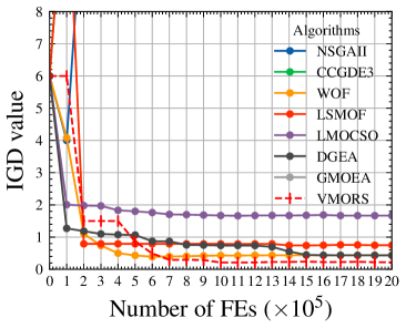
(b) 100,000 decision variables.

Figure 4: Convergence profiles of all compared algorithms on bi-objective LSMOP1 with 1,000 and 100,000 decision variables, respectively.

The variations of IGD values achieved by all compared algorithms on bi-objective LSMOP1 with 1,000 and 100,000 decision variables are presented in Figs. 4. (a) and (b), respectively. Due to the large differences between the results of some algorithms, in order to better show the gap between the better algorithms, the figure has been scaled. Consequently, the results of some algorithms in some figures are omitted.

It can be seen from the figures that most algorithms can solve LSMOP1 with 1000 decision variables, but when the problem is expanded to 100,000 dimensions, many algorithms cannot solve it. Specifically, NSGA-II and CCGDE3 fail to converge, whereas LSMOF, WOF, and DGEA have the ability to quickly search for a local optimum within small function evaluations, but fail to converge later. Only our proposed algorithm outputs a good result within the given limit of function evaluations.

IV-F Time complexity Analysis

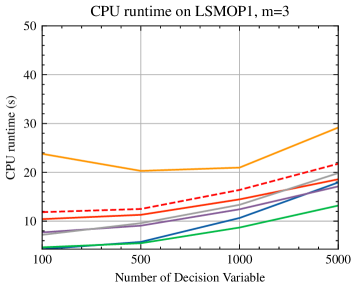
(a) The dimension of the decision variable varies from 100 to 20,000.

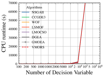
(b) The dimension of the decision variable varies from 100 to 1,000,000.

Figure 5: The running time of all compared algorithm in solving bi-objective LSMOP1, where FE=100,000. Please refer to Figs. S-1 to S-9 of the supplementary materials for all results.

TABLE VII: Value of IGD Metric Over Tri-Objective LSMOP Problems Obtained by Ablation Study, VMORS W/O DR is the method without recommending directions based on Thompson sampling, VMORS W/O VO is the method without directions fine-tuning method. The Best Result in Each Row is Highlighted in Bold.

Problem	D	W/O DR	W/O DF	VMORS	D	W/O DR	W/O Df	VMORS
LSMOP1	100	2.23e-01-	8.61e-01-	1.68e-01	2,000	1.38e-01+	8.61e-01-	1.92e-01
	200	2.13e-01=	8.61e-01-	1.66e-01	5,000	2.11e-01=	8.56e-01-	1.95e-01
	500	1.64e-01=	8.61e-01-	2.01e-01	10,000	1.96e-01+	8.61e-01-	2.50e-01
	1,000	1.85e-01=	8.61e-01-	2.29e-01	20,000	1.37e-01=	8.56e-01-	1.67e-01
LSMOP2	100	1.15e-01=	2.23e-01-	1.37e-01	2,000	7.14e-02=	9.42e-02=	6.26e-02
	200	9.93e-02=	1.37e-01=	9.52e-02	5,000	9.00e-02=	5.40e-02=	6.64e-02
	500	9.95e-02=	8.68e-02=	9.29e-02	10,000	8.12e-02=	1.52e-01-	8.76e-02
	1,000	9.37e-02=	7.48e-02=	9.55e-02	20,000	9.35e-02=	5.89e-02=	7.81e-02
LSMOP3	100	8.61e-01=	8.61e-01=	8.61e-01	2,000	8.61e-01=	8.61e-01=	8.61e-01
	200	8.61e-01=	8.61e-01=	8.61e-01	5,000	8.61e-01=	8.61e-01=	8.61e-01
	500	8.61e-01=	8.61e-01=	8.61e-01	10,000	8.61e-01=	8.61e-01=	8.61e-01
	1,000	8.61e-01=	8.61e-01=	8.57e-01	20,000	8.61e-01=	8.61e-01=	8.61e-01
LSMOP4	100	3.18e-01=	5.46e-01-	2.95e-01	2,000	8.86e-02=	1.14e-01=	7.66e-02
	200	2.42e-01=	3.73e-01-	2.10e-01	5,000	1.01e-01=	1.65e-01-	6.87e-02
	500	1.08e-01=	2.17e-01-	1.09e-01	10,000	5.91e-02=	6.72e-02=	8.54e-02
	1,000	9.26e-02=	1.41e-01=	9.49e-02	20,000	7.60e-02=	5.45e-02=	7.05e-02
LSMOP5	100	4.61e-01=	9.38e-01-	4.50e-01	2,000	4.80e-01=	9.46e-01-	5.00e-01
	200	4.63e-01=	7.19e-01-	4.51e-01	5,000	4.69e-01=	9.46e-01-	4.76e-01
	500	4.96e-01-	9.46e-01-	3.91e-01	10,000	4.98e-01=	9.46e-01-	5.28e-01
	1,000	4.71e-01=	9.46e-01-	4.86e-01	20,000	5.01e-01=	9.46e-01-	5.35e-01
LSMOP6	100	1.48e+00-	1.48e+00-	1.03e+00	2,000	1.09e+00-	1.70e+00-	7.68e-01
	200	8.90e-01+	1.59e+00-	1.23e+00	5,000	1.43e+00-	1.70e+00-	7.41e-01
	500	1.29e+00-	1.66e+00-	7.12e-01	10,000	7.33e-01+	1.70e+00-	8.29e-01
	1,000	1.31e+00=	1.69e+00-	1.31e+00	20,000	7.63e-01+	1.71e+00-	1.33e+00
LSMOP7	100	1.00e+00=	1.62e+00-	1.02e+00	2,000	8.42e-01=	9.79e-01-	8.41e-01
	200	9.48e-01=	1.59e+00-	9.37e-01	5,000	8.37e-01=	9.36e-01-	8.36e-01
	500	8.74e-01=	1.23e+00-	8.77e-01	10,000	8.35e-01=	1.71e+00-	8.35e-01
	1,000	8.51e-01=	1.06e+00-	8.47e-01	20,000	8.34e-01-	9.19e-01-	7.63e-01
LSMOP8	100	1.08e-01=	6.92e-01-	1.57e-01	2,000	9.48e-02=	5.01e-01-	1.08e-01
	200	1.18e-01=	6.41e-01-	1.37e-01	5,000	8.68e-02=	5.24e-01-	9.07e-02
	500	1.21e-01=	4.43e-01-	9.25e-02	10,000	8.03e-02=	5.44e-01-	8.66e-02
	1,000	1.02e-01=	5.61e-01-	1.04e-01	20,000	9.64e-02=	5.00e-01-	7.19e-02
LSMOP9	100	1.15e+00+	1.54e+00=	1.54e+00	2,000	1.14e+00-	1.53e+00-	5.87e-01
	200	1.54e+00=	1.52e+00=	1.54e+00	5,000	5.87e-01=	1.54e+00-	5.86e-01
	500	1.54e+00-	1.19e+00-	5.88e-01	10,000	1.14e+00-	1.54e+00-	5.88e-01
	1,000	5.88e-01+	1.54e+00=	1.54e+00	20,000	1.14e+00-	1.54e+00-	5.87e-01
(+/-/=)						7/11/54	0/51/21	32

For an algorithm to solve VLSMOPs and LSMOPs, its time complexity is an important evaluation index, and so time complexity is presented in Figs. 5. (a) and (b). The dimensions of the decision variables are from 100 to 5,000 and 100 to 1,000,000, respectively.

Firstly, it can be seen from Figs. 5. (a) and (b) that although the time complexity of our algorithm is not the lowest, nevertheless its complexity is not high,. Thus, the impact of dimensionality is relatively limited, and our algorithm belongs to the first tier of all running algorithms. Further, the rate with which the time complexity increases with the dimension of decision variables is close to most algorithms. Secondly, as can be seen from Fig. 5. (b), the time complexity of all algorithms increases dramatically from 20,000 dimensions to 100,000 dimensions, which simply illustrates that dealing with such large dimensions is a very challenging problem.

IV-G Ablation Study

In order to verify the effectiveness of directions recommendation and directions fine-tuning, we conduct an ablation experiment, which is reported in Table VII. We designed two variants of the VMORS algorithm, one without directions recommendation component (W/O DR), and one without directions fine-tuning component (W/O DF). The experiments are carried out on the tri-objective LSMOP problems, and the dimensions of the decision variables vary from 100 to 20,000 ($D\in\{100,200,500,1,000,2,000,5,000,10,000,20,000\}$).

First of all, it can be seen from Table VII that both variants of VMORS have the best results in some test instances, which shows that both components contribute to the improvement of the VMORS algorithm. Secondly, it can be seen from the final results that VMORS is dominant for both variants, and 32 out of 72 test cases obtained by VMORS are superior. This indicates that it is insufficient to solely recommend the direction or directly fine-tuning the direction. Only when directions recommendation and directions fine-tuning are combined at the same time can better results be achieved.

IV-H Parameter Sensitivity Analysis

In our proposed VMORS, a parameter $n_{d}$ is used to directly control the number of directions recommended by Thompson sampling, and this parameter also indirectly controls the number of direction population during evolution directions fine-tuning stage. To analyze the effect of this parameter on the performance of VMORS, experiments were conducted on a set of bi-objective LSMOP problems with 1.000 decision variables. The parameter $n_{d}$ is set to 5, 10, 20, 25, and 50, and the corresponding size of diversity solution is 20, 10, 5, 4, and 2. The experimental results are shown in Fig. 6. It can be observed that the performance of our proposed method is not significantly affected by different settings of $n_{d}$. This is especially true for the problems LSMOP2, LSMOP3, LSMOP4, LSMOP7, and LSMOP9, whilst for other problems, the performance has some fluctuation, but the result is still better compared to other state-of-the-art algorithms.

This result can be attributed to the fact that directions recommendation and directions fine-tuning are used simultaneously. When the number of recommended directions is insufficient, the size of direction population during the fine-tuning increases, thus compensating for the insufficient number of recommended directions. Conversely, when the size of direction population is insufficient, the number of recommended directions increases. Therefore, combined with the ablation experiments in the previous section, our proposed algorithm recommends direction and fine-tunes directions complementary to each other, improving the overall performance of the algorithm.

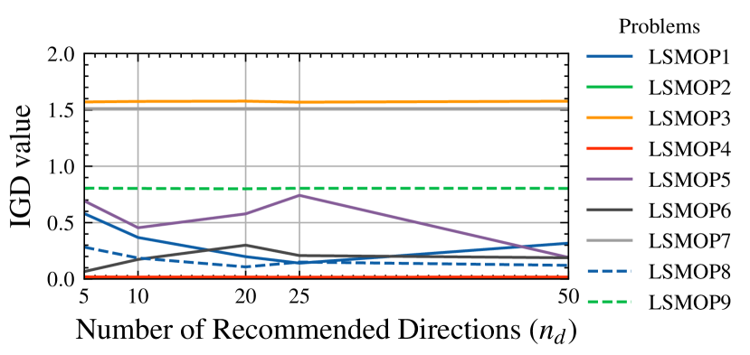
Figure 6: Statics of IGD results achieved by VMORS with different settings of the number of sampled directions $n_{d}$.

IV-I Discussion

A series of experiments have been conducted to verify the effectiveness of our algorithm. First, we select a series of representative MOEAs for comparison and tested on VLSMOPs and LSMOPs, our algorithm can obtain better results on most of the test instances. Second, we display the visualization of IGD variations and time complexity. Finally, we conducted ablation experiments and parameter sensitivity analysis on directions recommendation and directions fine-tuning. The results of these experiments verify that the two components both improve the search results, and that our method is not sensitive to these hyper-parameters.

V Conclusion and Future Work

Multiobjective optimization problems with an increasing number of decision variables can be found widely in industrial, economic, and scientific research. In this work, we formalize the notion of very large-scale multiobjective optimization problems with decision variables of more than 100,000, highlighting that these are actually quite prevalent in the real-world. Accordingly, we propose an algorithm that transforms and solves the problem of searching for directions in the very-large-scale decision variable space via a recommender system. The algorithm adopts Thompson sampling to recommend the direction that can guide the evolution of the population in the high-dimensional search space, and adopts the directions fine-tuning method to fine-tune the directions for solutions to evolve, so as to effectively solve very large-scale problems.

In a very large-scale decision space, the proposed algorithm does not search directly and evolve blindly in the high-dimensional space, but searches via the directions recommended by Thompson sampling. With recommended directions, the proposed algorithm designs the directions fine-tuning method to perform a finer-grained search based on the recommended direction, so as to avoid the problem that some optimal original spaces may not be reachable.

In order to verify the effectiveness of our algorithm, we compared the algorithm with the state-of-the-art algorithms on a wide range of benchmark instances. The experimental results verify that transforming such very large-scale problems into a recommender system is effective. Our work is an attempt to bridge between recommender systems and very large-scale optimization. In future work, introducing advanced recommender system methods and other techniques [50, 51, 52, 53] for solving MOP is still worth studying. In addition, as such very large-scale problems have wide practical application value, there is still much to explore on this important issue.

References

- [1] K. Deb, A. Pratap, S. Agarwal, and T. Meyarivan, “A fast and elitist multiobjective genetic algorithm: Nsga-ii,” IEEE Transactions on Evolutionary Computation, vol. 6, no. 2, pp. 182–197, 2002.
- [2] V. A. Shim, K. C. Tan, and H. Tang, “Adaptive memetic computing for evolutionary multiobjective optimization,” IEEE Transactions on Cybernetics, vol. 45, no. 4, pp. 610–621, 2015.
- [3] Y. Tian, L. Si, X. Zhang, R. Cheng, C. He, K. c. Tan, and Y. Jin, “Evolutionary large-scale multi-objective optimization: A survey,” ACM Computing Surveys, vol. 1, no. 1, 2021.
- [4] W.-J. Hong, P. Yang, and K. Tang, “Evolutionary computation for large-scale multi-objective optimization: A decade of progresses,” International Journal of Automation and Computing, pp. 1–15, 2021.
- [5] J. Liu, M. Gong, Q. Miao, X. Wang, and H. Li, “Structure learning for deep neural networks based on multiobjective optimization,” IEEE Transactions on Neural Networks and Learning Systems, vol. 29, no. 6, pp. 2450–2463, 2018.
- [6] Z. Yang, K. Tang, and X. Yao, “Large scale evolutionary optimization using cooperative coevolution,” Information Sciences, vol. 178, no. 15, pp. 2985–2999, 2008.
- [7] Y. Tian, X. Zhang, C. Wang, and Y. Jin, “An evolutionary algorithm for large-scale sparse multiobjective optimization problems,” IEEE Transactions on Evolutionary Computation, vol. 24, no. 2, pp. 380–393, 2020.
- [8] C. Qian, “Distributed pareto optimization for large-scale noisy subset selection,” IEEE Transactions on Evolutionary Computation, vol. 24, no. 4, pp. 694–707, Aug 2020.
- [9] Y. Tian, C. Lu, X. Zhang, K. C. Tan, and Y. Jin, “Solving large-scale multiobjective optimization problems with sparse optimal solutions via unsupervised neural networks,” IEEE Transactions on Cybernetics, vol. 51, no. 6, pp. 3115–3128, 2021.
- [10] H. Hong, M. Jiang, L. Feng, Q. Lin, and K. C. Tan, “Balancing exploration and exploitation for solving large-scale multiobjective optimization via attention mechanism,” in 2022 IEEE Congress on Evolutionary Computation (CEC), 2022, pp. 1–8.
- [11] L. M. Antonio and C. A. C. Coello, “Use of cooperative coevolution for solving large scale multiobjective optimization problems,” in 2013 IEEE Congress on Evolutionary Computation, 2013, pp. 2758–2765.
- [12] H. Zille, H. Ishibuchi, S. Mostaghim, and Y. Nojima, “A framework for large-scale multiobjective optimization based on problem transformation,” IEEE Transactions on Evolutionary Computation, vol. 22, no. 2, pp. 260–275, 2018.
- [13] C. He, S. Huang, R. Cheng, K. C. Tan, and Y. Jin, “Evolutionary multiobjective optimization driven by generative adversarial networks (gans),” IEEE Transactions on Cybernetics, pp. 1–14, 2020.
- [14] C. He, R. Cheng, C. Zhang, Y. Tian, Q. Chen, and X. Yao, “Evolutionary large-scale multiobjective optimization for ratio error estimation of voltage transformers,” IEEE Transactions on Evolutionary Computation, vol. 24, no. 5, pp. 868–881, 2020.
- [15] Z. Cui, X. Xu, F. XUE, X. Cai, Y. Cao, W. Zhang, and J. Chen, “Personalized recommendation system based on collaborative filtering for iot scenarios,” IEEE Transactions on Services Computing, vol. 13, no. 4, pp. 685–695, 2020.
- [16] R. A. Hamid, A. Albahri, J. K. Alwan, Z. Al-qaysi, O. Albahri, A. Zaidan, A. Alnoor, A. Alamoodi, and B. Zaidan, “How smart is e-tourism? a systematic review of smart tourism recommendation system applying data management,” Computer Science Review, vol. 39, p. 100337, 2021.
- [17] H. Hwangbo, Y. S. Kim, and K. J. Cha, “Recommendation system development for fashion retail e-commerce,” Electronic Commerce Research and Applications, vol. 28, pp. 94–101, 2018.
- [18] B. Lika, K. Kolomvatsos, and S. Hadjiefthymiades, “Facing the cold start problem in recommender systems,” Expert Systems with Applications, vol. 41, no. 4, Part 2, pp. 2065–2073, 2014.
- [19] D. J. Russo, B. Van Roy, A. Kazerouni, I. Osband, and Z. Wen, “A tutorial on thompson sampling,” Found. Trends Mach. Learn., vol. 11, no. 1, p. 1–96, jul 2018.
- [20] Y. Tian, X. Zheng, X. Zhang, and Y. Jin, “Efficient large-scale multiobjective optimization based on a competitive swarm optimizer,” IEEE Transactions on Cybernetics, vol. 50, no. 8, pp. 3696–3708, 2020.
- [21] Y. Tian, Y. Feng, X. Zhang, and C. Sun, “A fast clustering based evolutionary algorithm for super-large-scale sparse multi-objective optimization,” IEEE/CAA Journal of Automatica Sinica, pp. 1–16, 2022.
- [22] L. Li, C. He, R. Cheng, H. Li, L. Pan, and Y. Jin, “A fast sampling based evolutionary algorithm for million-dimensional multiobjective optimization,” Swarm and Evolutionary Computation, vol. 75, p. 101181, 2022.
- [23] L. M. Antonio, C. A. C. Coello, S. G. Brambila, J. F. González, and G. C. Tapia, “Operational decomposition for large scale multi-objective optimization problems,” in Proceedings of the Genetic and Evolutionary Computation Conference Companion, ser. GECCO ’19. New York, NY, USA: Association for Computing Machinery, 2019, p. 225–226.
- [24] F. Sander, H. Zille, and S. Mostaghim, “Transfer strategies from single- to multi-objective grouping mechanisms,” in Proceedings of the Genetic and Evolutionary Computation Conference, ser. GECCO ’18. New York, NY, USA: Association for Computing Machinery, 2018, p. 729–736.
- [25] H. Chen, X. Zhu, W. Pedrycz, S. Yin, G. Wu, and H. Yan, “Pea: Parallel evolutionary algorithm by separating convergence and diversity for large-scale multi-objective optimization,” in 2018 IEEE 38th International Conference on Distributed Computing Systems (ICDCS), 2018, pp. 223–232.
- [26] X. Ma, F. Liu, Y. Qi, X. Wang, L. Li, L. Jiao, M. Yin, and M. Gong, “A multiobjective evolutionary algorithm based on decision variable analyses for multiobjective optimization problems with large-scale variables,” IEEE Transactions on Evolutionary Computation, vol. 20, no. 2, pp. 275–298, 2016.
- [27] X. Zhang, Y. Tian, R. Cheng, and Y. Jin, “A decision variable clustering-based evolutionary algorithm for large-scale many-objective optimization,” IEEE Transactions on Evolutionary Computation, vol. 22, no. 1, pp. 97–112, 2018.
- [28] H. Qian and Y. Yu, “Solving high-dimensional multi-objective optimization problems with low effective dimensions,” in Proceedings of the Thirty-First AAAI Conference on Artificial Intelligence, ser. AAAI’17. AAAI Press, 2017, p. 875–881.
- [29] R. Liu, R. Ren, J. Liu, and J. Liu, “A clustering and dimensionality reduction based evolutionary algorithm for large-scale multi-objective problems,” Applied Soft Computing, vol. 89, p. 106120, 2020.
- [30] C. He, L. Li, Y. Tian, X. Zhang, R. Cheng, Y. Jin, and X. Yao, “Accelerating large-scale multiobjective optimization via problem reformulation,” IEEE Transactions on Evolutionary Computation, vol. 23, no. 6, pp. 949–961, 2019.
- [31] J.-H. Yi, L.-N. Xing, G.-G. Wang, J. Dong, A. V. Vasilakos, A. H. Alavi, and L. Wang, “Behavior of crossover operators in nsga-iii for large-scale optimization problems,” Information Sciences, vol. 509, pp. 470–487, 2020.
- [32] C. He, R. Cheng, and D. Yazdani, “Adaptive offspring generation for evolutionary large-scale multiobjective optimization,” IEEE Transactions on Systems, Man, and Cybernetics: Systems, pp. 1–13, 2020.
- [33] S. Qin, C. Sun, Y. Jin, Y. Tan, and J. Fieldsend, “Large-scale evolutionary multiobjective optimization assisted by directed sampling,” IEEE Transactions on Evolutionary Computation, vol. 25, no. 4, pp. 724–738, 2021.
- [34] W. Hong, K. Tang, A. Zhou, H. Ishibuchi, and X. Yao, “A scalable indicator-based evolutionary algorithm for large-scale multiobjective optimization,” IEEE Transactions on Evolutionary Computation, vol. 23, no. 3, pp. 525–537, 2019.
- [35] Z. Wang, H. Hong, K. Ye, G.-E. Zhang, M. Jiang, and K. C. Tan, “Manifold interpolation for large-scale multiobjective optimization via generative adversarial networks,” IEEE Transactions on Neural Networks and Learning Systems, pp. 1–15, 2021.
- [36] C. Gao, W. Lei, X. He, M. de Rijke, and T.-S. Chua, “Advances and challenges in conversational recommender systems: A survey,” AI Open, vol. 2, pp. 100–126, 2021.
- [37] Q. Zhang, J. Lu, and Y. Jin, “Artificial intelligence in recommender systems,” Complex Intelligent Systems, vol. 7, no. 1, pp. 439–457, 2021.
- [38] S. Li, W. Lei, Q. Wu, X. He, P. Jiang, and T.-S. Chua, “Seamlessly unifying attributes and items: Conversational recommendation for cold-start users,” ACM Trans. Inf. Syst., vol. 39, no. 4, aug 2021.
- [39] O. Chapelle and L. Li, “An empirical evaluation of thompson sampling,” in Advances in Neural Information Processing Systems, J. Shawe-Taylor, R. Zemel, P. Bartlett, F. Pereira, and K. Weinberger, Eds., vol. 24. Curran Associates, Inc., 2011.
- [40] W. R. Thompson, “On the likelihood that one unknown probability exceeds another in view of the evidence of two samples,” Biometrika, vol. 25, no. 3/4, pp. 285–294, 1933.
- [41] W. R. Thompson, “On the theory of apportionment,” American Journal of Mathematics, vol. 57, no. 2, pp. 450–456, 1935.
- [42] L. Sun and K. Li, “Adaptive operator selection based on dynamic thompson sampling for moea/d,” in Parallel Problem Solving from Nature – PPSN XVI, T. Bäck, M. Preuss, A. Deutz, H. Wang, C. Doerr, M. Emmerich, and H. Trautmann, Eds. Cham: Springer International Publishing, 2020, pp. 271–284.
- [43] N. Gupta, O.-C. Granmo, and A. Agrawala, “Thompson sampling for dynamic multi-armed bandits,” in 2011 10th International Conference on Machine Learning and Applications and Workshops, vol. 1, 2011, pp. 484–489.
- [44] C. He, S. Huang, R. Cheng, K. C. Tan, and Y. Jin, “Evolutionary multiobjective optimization driven by generative adversarial networks (gans),” IEEE Transactions on Cybernetics, vol. 51, no. 6, pp. 3129–3142, 2021.
- [45] Y. Tian, R. Cheng, X. Zhang, and Y. Jin, “Platemo: A matlab platform for evolutionary multi-objective optimization [educational forum],” IEEE Computational Intelligence Magazine, vol. 12, no. 4, pp. 73–87, 2017.
- [46] R. Cheng, Y. Jin, M. Olhofer, and B. Sendhoff, “Test problems for large-scale multiobjective and many-objective optimization,” IEEE Transactions on Cybernetics, vol. 47, no. 12, pp. 4108–4121, 2017.
- [47] E. Zitzler, L. Thiele, M. Laumanns, C. M. Fonseca, and V. G. d. Fonseca, “Performance assessment of multiobjective optimizers: an analysis and review,” IEEE Transactions on Evolutionary Computation, vol. 7, no. 2, pp. 117–132, 2003.
- [48] L. While, P. Hingston, L. Barone, and S. Huband, “A faster algorithm for calculating hypervolume,” IEEE Transactions on Evolutionary Computation, vol. 10, no. 1, pp. 29–38, 2006.
- [49] W. Haynes, Wilcoxon Rank Sum Test. New York, NY: Springer New York, 2013, pp. 2354–2355.
- [50] M. Jiang, Z. Wang, L. Qiu, S. Guo, X. Gao, and K. C. Tan, “A fast dynamic evolutionary multiobjective algorithm via manifold transfer learning,” IEEE Transactions on Cybernetics, vol. 51, no. 7, pp. 3417–3428, 2021.
- [51] M. Jiang, Z. Wang, S. Guo, X. Gao, and K. C. Tan, “Individual-based transfer learning for dynamic multiobjective optimization,” IEEE Transactions on Cybernetics, vol. 51, no. 10, pp. 4968–4981, 2021.
- [52] J. Ang, K. Tan, and A. Mamun, “An evolutionary memetic algorithm for rule extraction,” Expert Systems with Applications, vol. 37, no. 2, pp. 1302–1315, 2010. [Online]. Available: https://www.sciencedirect.com/science/article/pii/S0957417409005545
- [53] X. Qiu, J.-X. Xu, Y. Xu, and K. C. Tan, “A new differential evolution algorithm for minimax optimization in robust design,” IEEE Transactions on Cybernetics, vol. 48, no. 5, pp. 1355–1368, 2018.