A Riemannian Proximal Newton Method

Abstract

In recent years, the proximal gradient method and its variants have been generalized to Riemannian manifolds for solving optimization problems with an additively separable structure, i.e., $f+h$, where $f$ is continuously differentiable, and $h$ may be nonsmooth but convex with computationally reasonable proximal mapping. In this paper, we generalize the proximal Newton method to embedded submanifolds for solving the type of problem with $h(x)=\mu\|x\|_{1}$. The generalization relies on the Weingarten and semismooth analysis. It is shown that the Riemannian proximal Newton method has a local superlinear convergence rate under certain reasonable assumptions. Moreover, a hybrid version is given by concatenating a Riemannian proximal gradient method and the Riemannian proximal Newton method. It is shown that if the objective function satisfies the Riemannian KL property and the switch parameter is chosen appropriately, then the hybrid method converges globally and also has a local superlinear convergence rate. Numerical experiments on random and synthetic data are used to demonstrate the performance of the proposed methods.

1   Introduction

In this paper, we consider the following optimization problem

$$\min_{x\in\operatorname{\mathcal{M}}}F(x)=f(x)+h(x),$$ (1.1)

where $\operatorname{\mathcal{M}}$ is a finite-dimensional embedded submanifold of a Euclidean space, see Definition 2.1, $f$ is a sufficiently smooth function, and the function

$$h(x)=\mu\|x\|_{1}$$

with $\mu$ being positive. This optimization problem arises in many important applications, such as sparse principal component analysis [ZHT06, ZX18], sparse partial least squares regression [CSG⁺19], compressed model [OLCO13], sparse inverse covariance estimation [BESS19], sparse blind deconvolution [ZLwK⁺17] and clustering [LYL16, PZ18, HWGD22].

In the case that the manifold constraint is dropped, i.e., $\operatorname{\mathcal{M}}=\operatorname{\mathbb{R}}^{n}$, and the function $h$ is not restricted to be $\mu\|x\|_{1}$ but a continuous, convex, and not necessarily smooth function, the Euclidean nonsmooth problem (1.1) has been extensively studied in [Bec17, Nes18]. The well-known methods include the proximal gradient method and its variants, which have found many practical successes in applications [SYGL14, BT09a, Tib96, WOR12]. The proximal gradient method updates the iterate via

$$\begin{cases}v_{k}=\operatorname*{argmin}_{v\in\operatorname{\mathbb{R}}^{n}}\ f(x_{k})+\nabla f(x_{k})^{\operatorname{\mathrm{T}}}v+\frac{1}{2t}\|v\|_{\operatorname{\mathrm{F}}}^{2}+h(x_{k}+v),&\text{ (Proximal mapping) }\\ x_{k+1}=x_{k}+v_{k},&\text{ (Update iterates) }\end{cases}$$ (1.2)

where the proximal mapping in (1.2) uses the first-order approximation of $f$ around the current estimate $x_{k}$. If the function $f$ is convex, then under certain standard assumptions, the proximal gradient method has an $\mathcal{O}(1/k)$ rate of convergence [Bec17, Chapter 10]. Moreover, multiple accelerated versions of the proximal gradient method have been proposed in [BT09b, VSBV13, LL15, AP16], which achieve the optimal convergence rate $\mathcal{O}(1/k^{2})$ [Nes83]. If the function $f$ is further assumed to be strongly convex, then the convergence rate of the proximal gradient method can be shown to be linear.

With the presence of the manifold constraint, the nonsmooth optimization problem (1.1) becomes more challenging. The update iterates in (1.2) can be generalized to the Riemannian setting using a standard technique called retraction. However, generalizing the proximal mapping in (1.2) to the Riemannian setting is not straightforward, and multiple versions have been proposed. In [CMSZ20], a proximal gradient method called ManPG for solving the optimization problem over the Stiefel manifold is proposed and the update parallel to (1.2) is given by

$$\begin{cases}v_{k}=\operatorname*{argmin}_{v\in\operatorname{\mathrm{T}}_{x_{k}}\operatorname{\mathcal{M}}}\ f(x_{k})+\nabla f(x_{k})^{\operatorname{\mathrm{T}}}v+\frac{1}{2t}\|v\|_{\operatorname{\mathrm{F}}}^{2}+h(x_{k}+v),&\text{ (Proximal mapping) }\\ x_{k+1}=R_{x_{k}}(v_{k}).&\text{ (Update iterates) }\end{cases}$$ (1.3)

Compared to the Euclidean setting, the Riemannian proximal mapping in (1.3) has an additional linear constraint that ensures the search direction $v_{k}$ stays in the tangent space $\operatorname{\mathrm{T}}_{x_{k}}\operatorname{\mathcal{M}}$. It is shown in [CMSZ20, Section 4.2] that the proximal mapping in (1.3) can be solved efficiently by a semismooth Newton method. Moreover, the global convergence of ManPG has been established. In [HW22a], a diagonal weighted proximal mapping is defined by replacing $\|v\|_{\operatorname{\mathrm{F}}}^{2}$ in (1.3) by $\langle v,Wv\rangle$, where the diagonal weighted linear operator $W$ is motivated from the Hessian. In addition, an accelerated proximal gradient method is generalized to the Riemannian setting called AManPG that empirically exhibits accelerated behavior over the Stiefel manifold. The Riemannian generalization of the proximal mapping in (1.3) requires being able to perform a linear combination of $x_{k}+v$, which cannot be defined on a generic manifold. In [HW22b], a Riemannian gradient method called RPG is proposed by replacing the addition $x_{k}+v$ with a retraction $R_{x_{k}}(v)$, which yields a Riemannian proximal mapping

$$v_{k}=\operatorname*{argmin}_{v\in\operatorname{\mathrm{T}}_{x_{k}}\operatorname{\mathcal{M}}}\ f(x_{k})+\langle\operatorname{\mathrm{grad}}f(x_{k}),v\rangle_{x_{k}}+\frac{1}{2t}\|v\|_{x_{k}}^{2}+h\left(R_{x_{k}}(v)\right)$$ (1.4)

where $\operatorname{\mathrm{grad}}f$ denotes the Riemannian gradient of $f$ and $\langle\cdot,\cdot\rangle_{x}$ is Riemannian metric defined on the tangent space $\operatorname{\mathrm{T}}_{x}\operatorname{\mathcal{M}}$. Not only the global convergence but also the local convergence rate has been established in terms of the Riemannian KL property. The same authors further propose the inexact Riemannian proximal gradient method called IRPG without solving (1.4) exactly in [HW23]. The global convergence and local convergence rates have also been given. Moreover, the search direction given by (1.3) can be viewed as an inexact solution of the Riemannian proximal mapping (1.4) that still guarantees global convergence. Though the Riemannian proximal gradient method with (1.4) has nice global and local convergence results, it is still unknown whether Subproblem (1.4) can be solved efficiently in general.

If $\operatorname{\mathcal{M}}=\operatorname{\mathbb{R}}^{n}$ and the function $f$ is twice continuously differentiable and strongly convex, proximal Newton-type methods are proposed in [LSS14] and achieve a superlinear convergence rate. The proximal mapping in the proximal Newton-type methods replaces $f$ with a second-order approximation and yields the search direction

$$v_{k}=\operatorname*{argmin}_{v\in\operatorname{\mathbb{R}}^{n}}\ f(x_{k})+\nabla f(x_{k})^{\operatorname{\mathrm{T}}}v+\frac{1}{2}v^{\operatorname{\mathrm{T}}}H_{k}v+h(x_{k}+v),$$ (1.5)

where $H_{k}$ represents a suitable approximation of the exact Hessian $\nabla^{2}f(x_{k})$. If $H_{k}$ is chosen to be the Hessian, i.e., $H_{k}=\nabla^{2}f(x_{k})$, then the search direction (1.5) yields the proximal Newton method. The Euclidean proximal Newton-type method traces its prototype back to [Jos79a, Jos79b], where it was primarily used to solve generalized equations. Over the next few decades, this method was extensively studied and has been proven to be efficient and effective in many applications [PJL⁺13, ZYDR14, KV17, SSS18, AGO20]. In the Euclidean setting, if the function $f$ is twice continuously differentiable and strongly convex, the Hessian of $f$ is Lipschitz continuous, and the function $h$ is convex, then the proximal Newton method converges quadratically. When generalizing to the Riemannian setting, some of the assumptions may be too strong. For example, a geodesically-convex function, which is a commonly-used Riemannian generalization of convexity, on a compact manifold must be a constant function, see [Bou23, Corollary 11.10]. In [MYZZ23], the authors remove the global convexity of $f$ of the Euclidean proximal Newton method while still guaranteeing global convergence and local superlinear convergence. However, the manifold curvature appears in the second-order information of the objective function, which still significantly increases the difficulty of generalizing to the Riemannian setting. The recent paper [WY23] proposes the proximal quasi-Newton method, called ManPQN, over the Stiefel manifold with the Riemannian proximal mapping

$$v_{k}=\operatorname*{argmin}_{v\in\operatorname{\mathrm{T}}_{x_{k}}\operatorname{\mathcal{M}}}\ f(x_{k})+\langle\operatorname{\mathrm{grad}}f(x_{k}),v\rangle+\frac{1}{2}\|v\|_{\mathcal{B}_{k}}^{2}+h\left(x_{k}+v\right),$$ (1.6)

where $\mathcal{B}_{k}$ is a symmetric positive definite operator on $\operatorname{\mathrm{T}}_{x_{k}}\operatorname{\mathcal{M}}$ and $\|v\|_{\mathcal{B}_{k}}^{2}=\langle v,\mathcal{B}_{k}[v]\rangle$. Additionally, the global convergence of ManPQN has been established. However, in both theoretical and numerical results, only the local linear convergence of ManPQN has been demonstrated. Note that the naive generalization of replacing the Euclidean gradient and Hessian with the Riemannian counterparts generally does not yield a superlinear convergence result, see details in Section 5.1.

The main contributions of this paper are summarized as follows. A Riemannian proximal Newton method, called RPN, is proposed and studied. This method is based on the idea of semismooth implicit function analysis, which is different from the naive generalization of Euclidean setting [LSS14]. It is proven that the proposed algorithm is capable of achieving superlinear convergence under certain reasonable assumptions. The local result requires that the iterative point is sufficiently close to an optimal point. We show that the distance between the iterative point and the optimal point can be controlled by the norm of search direction. Therefore, a hybrid version by concatenating a Riemannian proximal gradient method and the Riemannian proximal Newton method is given, and its global and local superlinear convergence is guaranteed. Numerical experiments are used to demonstrate the performance of the proposed methods.

This paper is organized as follows. Notation and preliminaries are given in Section 2. The Riemannian proximal Newton method together with its local convergence analyzes are presented in Section 3. The hybrid algorithm is described and analyzed in Section 4. Numerical experiments are reported in Section 5. Finally, we draw some concluding remarks and potential future directions in Section 6.

2   Notation and Preliminaries

2.1 Preliminaries on Riemannian Submanifolds of Euclidean Spaces

An $n$-dimensional Euclidean space is denoted by $\operatorname{\mathbb{R}}^{n}$. The Euclidean space $\operatorname{\mathbb{R}}^{n}$ does not only refer to a vector space, but also can refer to a matrix space or a tensor space. In a Euclidean space, the Euclidean metric is typically represented by $\langle u,v\rangle$, which is defined as the sum of the entry-wise products of $u$ and $v$, such as $u^{\operatorname{\mathrm{T}}}v$ for vectors and $\operatorname{\mathrm{trace}}(u^{\operatorname{\mathrm{T}}}v)$ for matrices. The Frobenius norm is denoted by $\|\cdot\|_{\operatorname{\mathrm{F}}}=\sqrt{{\langle\cdot,\cdot\rangle}}$. A linear operator $\mathcal{A}$ on the Euclidean space $\operatorname{\mathbb{R}}^{n}$ is call self-adjoint or symmetric if it satisfies ${\langle\mathcal{A}x,y\rangle}={\langle x,\mathcal{A}y\rangle}$, for all $x,y\in\operatorname{\mathbb{R}}^{n}$. If a symmetric linear operator $\mathcal{A}$ satisfies ${\langle\mathcal{A}x,x\rangle}>(\geq)0$ for all $x\in\operatorname{\mathbb{R}}^{n}\setminus\{0\}$, then $\mathcal{A}$ is called a symmetric positive definite (semidefinite) linear operator and denoted by $\mathcal{A}\succ(\succeq)0$. For $x\in\operatorname{\mathbb{R}}^{n}$, $\|x\|_{1}$ denotes the sum of the absolute values of all entries in $x$ and $\operatorname{\mathrm{sgn}}(x)\in\operatorname{\mathbb{R}}^{n}$ denotes the sign function, i.e.,

$$(\operatorname{\mathrm{sgn}}(x))_{i}:=\begin{cases}-1&\text{ if }x_{i}<0,\\ 0&\text{ if }x_{i}=0,\\ 1&\text{ if }x_{i}>0.\end{cases}$$

For $x,y\in\mathbb{R}^{n}$, $x\odot y$ denotes $z\in\mathbb{R}^{n}$ such that $z_{i}=x_{i}y_{i}$ for all $i$, that is, $\odot$ denotes the Hadamard product.

The following is the standard definition of an embedded submanifold [AMS08, Bou23], which is used in the proof of Lemma 3.8. Roughly speaking, an embedded submanifold in an Euclidean space is either an open subset or a smooth surface in the space.

Definition 2.1 (Embedded submanifolds of $\operatorname{\mathbb{R}}^{n}$ [Bou23] ).

Let $\operatorname{\mathcal{M}}$ be a subset of a Euclidean space $\operatorname{\mathbb{R}}^{n}$. We say $\operatorname{\mathcal{M}}$ is a (smooth) embedded submanifold of $\operatorname{\mathbb{R}}^{n}$ if either $\mathcal{M}$ is an open subset of $\operatorname{\mathbb{R}}^{n}$ or for a fixed integer $k\geq 1$ and for each $x\in\operatorname{\mathcal{M}}$ there exists a neighbourhood $\mathcal{U}$ of $x$ in $\operatorname{\mathbb{R}}^{n}$ and a smooth function $h:\mathcal{U}\to\operatorname{\mathbb{R}}^{k}$ such that

• If $y$ is in $\mathcal{U}$, then $h(y)=0$ if and only if $y\in\mathcal{M}$; and

• $\operatorname{rank}\mathrm{D}h(x)=k$,

where $\mathrm{D}$ denotes the differential operator. Such a function $h$ is called a local defining function for $\operatorname{\mathcal{M}}$ at $x$.

The tangent space of the manifold $\operatorname{\mathcal{M}}$ at $x$ is denoted by $\operatorname{\mathrm{T}}_{x}\operatorname{\mathcal{M}}$, and the tangent bundle, denoted $\operatorname{\mathrm{T}}\operatorname{\mathcal{M}}$, is the set of all tangent vectors. Since the tangent space is a vector space, one can equip it with an inner product (or metric) $\langle\cdot,\cdot\rangle_{x}:\operatorname{\mathrm{T}}_{x}\operatorname{\mathcal{M}}\times\operatorname{\mathrm{T}}_{x}\operatorname{\mathcal{M}}\to\operatorname{\mathbb{R}}$. A manifold whose tangent spaces are endowed with a smoothly varying metric is referred to as a Riemannian manifold. If the manifold $\operatorname{\mathcal{M}}$ is an embedded submanifold of $\operatorname{\mathbb{R}}^{n}$ and the Riemannian metric of $\operatorname{\mathcal{M}}$ is endowed from $\operatorname{\mathbb{R}}^{n}$, then $\operatorname{\mathcal{M}}$ is called a Riemannian submanifold of $\operatorname{\mathbb{R}}^{n}$.

When the manifold $\operatorname{\mathcal{M}}$ is an embedded submanifold of $\operatorname{\mathbb{R}}^{n}$, the tangent space $\operatorname{\mathrm{T}}_{x}\operatorname{\mathcal{M}}$ is a linear subspace of $\operatorname{\mathbb{R}}^{n}$. One can define the orthogonal complement space of $\operatorname{\mathrm{T}}_{x}\operatorname{\mathcal{M}}$ as $\operatorname{\mathrm{N}}_{x}\operatorname{\mathcal{M}}=\operatorname{\mathrm{T}}_{x}^{\perp}\operatorname{\mathcal{M}}$, called the normal space of $\operatorname{\mathcal{M}}$ at $x$. If one can find a basis of $\operatorname{\mathrm{N}}_{x}\operatorname{\mathcal{M}}$, denoted by $B_{x}=\left(b_{x}^{(1)},b_{x}^{(2)},\ldots,b_{x}^{(d)}\right)$, then the tangent space $\operatorname{\mathrm{T}}_{x}\operatorname{\mathcal{M}}$ can be characterized as its orthogonal complement

$$\operatorname{\mathrm{T}}_{x}\operatorname{\mathcal{M}}=\{v\in\mathbb{R}^{n}:B_{x}^{T}v:=\left({\langle b_{x}^{(1)},v\rangle},{\langle b_{x}^{(2)},v\rangle},\ldots,{\langle b_{x}^{(d)},v\rangle}\right)^{T}=0\}.$$

Moreover, the basis $B_{x}$ can be built as a smooth function of $x$ in a neighborhood of $x$ for any $x\in\operatorname{\mathcal{M}}$, see [HAG17]. We will see in Section 3, that such a characterization of $\operatorname{\mathrm{T}}_{x}\operatorname{\mathcal{M}}$ is useful in reformulating Riemannian proximal mappings.

The Riemannian gradient of a smooth function $f:\operatorname{\mathcal{M}}\to\operatorname{\mathbb{R}}$ at $x$, denoted by $\operatorname{\mathrm{grad}}f(x)$, is the unique tangent vector satisfying

$$\mathrm{D}f(x)[\eta_{x}]=\left\langle\eta_{x},\operatorname{\mathrm{grad}}f(x)\right\rangle_{x},\ \forall\eta_{x}\in\operatorname{\mathrm{T}}_{x}\operatorname{\mathcal{M}},$$ (2.1)

where $\langle\cdot,\cdot\rangle_{x}$ is the Riemannian metric on $\operatorname{\mathrm{T}}_{x}\operatorname{\mathcal{M}}$ and $\mathrm{D}f(x)[\eta_{x}]$ is the directional derivative of $f$ at $x$ along $\eta_{x}$. If $\operatorname{\mathcal{M}}$ is a Riemannian submanifold of $\operatorname{\mathbb{R}}^{n}$, then Riemannian gradient $\operatorname{\mathrm{grad}}f(x)$ has the following explicit statement,

$$\operatorname{\mathrm{grad}}f(x)=\operatorname{\mathrm{Proj}}_{x}\left(\nabla f(x)\right),$$

where $\nabla f(x)$ is the Euclidean gradient, $\operatorname{\mathrm{Proj}}_{x}$ denotes the orthogonal projector onto $\operatorname{\mathrm{T}}_{x}\operatorname{\mathcal{M}}$, and the orthogonality is defined by the Euclidean metric.

The Riemannian Hessian of $f$ at $x$, denoted by $\operatorname{\mathrm{Hess}}f(x)$, is a linear operator on $\operatorname{\mathrm{T}}_{x}\operatorname{\mathcal{M}}$ satisfying

$$\operatorname{\mathrm{Hess}}f(x)[\eta_{x}]=\bar{\nabla}_{\eta_{x}}\operatorname{\mathrm{grad}}f(x),\ \forall\eta_{x}\in\operatorname{\mathrm{T}}_{x}\operatorname{\mathcal{M}},$$

where $\operatorname{\mathrm{Hess}}f(x)[\eta_{x}]$ denotes the action of $\operatorname{\mathrm{Hess}}f(x)$ on a tangent vector $\eta_{x}$, and $\bar{\nabla}$ denotes the Riemannian affine connection, see [AMS08, Section 5.3] and [Bou23, Section 5.4]. Roughly speaking, an affine connection generalizes the concept of a directional derivative of a vector field. Furthermore, if $\operatorname{\mathcal{M}}$ is a Riemannian submanifold of $\operatorname{\mathbb{R}}^{n}$, then the action of Riemannian Hessian $\operatorname{\mathrm{Hess}}f(x)$ along the direction $\eta_{x}\in\operatorname{\mathrm{T}}_{x}\operatorname{\mathcal{M}}$ has the following explicit expression, see [Bou23, Section 5.5 and 5.11], i.e.,

$$\operatorname{\mathrm{Hess}}f(x)[\eta_{x}]=\operatorname{\mathrm{Proj}}_{x}\left(\mathrm{D}\operatorname{\mathrm{grad}}f(x)[\eta_{x}]\right)=\operatorname{\mathrm{Proj}}_{x}\left(\nabla^{2}f(x)[\eta_{x}]\right)+\operatorname{\mathcal{W}}_{x}\left(\eta_{x},\operatorname{\mathrm{Proj}}_{x}^{\perp}\big{(}\nabla f(x)\big{)}\right),$$ (2.2)

where $\nabla^{2}f(x)$ is the Euclidean Hessian, $\operatorname{\mathrm{Proj}}_{x}^{\perp}=\mathrm{Id}-\operatorname{\mathrm{Proj}}_{x}$ is the orthogonal projector to the normal space $\operatorname{\mathrm{N}}_{x}\operatorname{\mathcal{M}}=(\operatorname{\mathrm{T}}_{x}\operatorname{\mathcal{M}})^{\perp}$, $\mathrm{Id}$ denotes the identity operator, $\operatorname{\mathcal{W}}_{x}$ is the Weingarten map [Bou23, Section 5.11] defined by

$$\operatorname{\mathcal{W}}_{x}:\operatorname{\mathrm{T}}_{x}\operatorname{\mathcal{M}}\times\operatorname{\mathrm{N}}_{x}\operatorname{\mathcal{M}}\to\operatorname{\mathrm{T}}_{x}\operatorname{\mathcal{M}}:(w,u)\mapsto\operatorname{\mathcal{W}}_{x}(w,u)=\operatorname{\mathrm{D}}(x\mapsto\operatorname{\mathrm{Proj}}_{x})(x)[w]\cdot u,$$ (2.3)

where $\operatorname{\mathrm{D}}(x\mapsto\operatorname{\mathrm{Proj}}_{x})(x)$ is the differential of the function $\operatorname{\mathrm{Proj}}_{x}$ at $x$. The Weingarten map is related to the curvature of the manifold, see [Lee18, Chapter 8].

A retraction on a manifold $\operatorname{\mathcal{M}}$ is a smooth mapping from the tangent bundle $\operatorname{\mathrm{T}}\operatorname{\mathcal{M}}$ to $\operatorname{\mathcal{M}}$ such that $(i)R_{x}(0_{x})=x$, where $0_{x}$ is the zero vector in $\operatorname{\mathrm{T}}_{x}\operatorname{\mathcal{M}}$; $(ii)$ the differential of $R_{x}$ at $0_{x}$, denoted $\mathrm{D}R_{x}(0_{x})$, is the identity map. Although the domain of a retraction does not necessarily need to be the whole tangent bundle, it is often the case in practice. Retractions whose domain is the whole tangent bundle are referred to as globally defined retractions. We denote $R_{x}:\operatorname{\mathrm{T}}_{x}\operatorname{\mathcal{M}}\to\operatorname{\mathcal{M}}$ to be the restriction of $R$ to $\operatorname{\mathrm{T}}_{x}M$. For any $x\in\operatorname{\mathcal{M}}$, there always exists a neighborhood of $0_{x}$ such that $R_{x}$ is a diffeomorphism in the neighborhood.

If the manifold $\operatorname{\mathcal{M}}$ is compact and the function $f$ is smooth, then it is known that the function $f$ satisfies a Riemannian version of smoothness. The details are given in Lemma 2.2.

Lemma 2.2 ( [BAC19]).

Let $\operatorname{\mathcal{M}}$ be a compact Riemannian submanifold of $\operatorname{\mathbb{R}}^{n}$. Suppose that the retraction $R$ on $\operatorname{\mathcal{M}}$ is globally defined, that is, $R_{x}(\eta_{x})$ is well defined for any $\eta_{x}\in\operatorname{\mathrm{T}}_{x}\mathcal{M}$. If $f:\operatorname{\mathbb{R}}^{n}\to\operatorname{\mathbb{R}}$ has Lipschitz continuous gradient in the convex hull of $\operatorname{\mathcal{M}}$, then we have

$$\left|f(R_{x}(\eta_{x}))-f(x)-\langle\operatorname{\mathrm{grad}}f(x),\eta_{x}\rangle\right|\leq\frac{L_{f}}{2}\|\eta_{x}\|^{2},$$ (2.4)

for all $\eta_{x}\in\operatorname{\mathrm{T}}_{x}\operatorname{\mathcal{M}}$ with constant $L_{f}$ independent of $x$.

2.2 Preliminaries on Implicit Function Theorems

The proposed proximal Newton method relies on an implicit function theorem for semismooth functions. In this section, the implicit function theorems for both smooth and semismooth functions are reviewed. We refer interested readers to [KP02, DRR09, Sun01, PSS03, Gow04] for more details. Lemma 2.3 states the well-known implicit function theorem for continuously differentiable functions.

Lemma 2.3 (Implicit Function Theorem).

Let $F:\mathbb{R}^{n+m}\to\mathbb{R}^{m}$ be a continuously differentiable (i.e., $\mathbb{C}^{1}$) function, and $F(x^{0},y^{0})=0$. If the Jacobian matrix $J_{y}F(x^{0},y^{0})$ is invertible, then there exists an open set $U\subset\mathbb{R}^{n}$ containing $x^{0}$ such that there exists a unique $\mathbb{C}^{1}$ function $f:U\to\mathbb{R}^{m}$ such that $f(x^{0})=y^{0}$, and $F(x,f(x))=0$ for all $x\in U$. Moreover, the Jacobian matrix of partial derivatives of $f$ in $U$ are given by the matrix product $Jf(x)=-[J_{y}F(x,y)]^{-1}J_{x}F(x,y).$

However, in many applications we encounter functions that are not differentiable everywhere, which leads to the following definition of semismoothness.

Definition 2.4 (Semismoothness [QS93, LST18]).

Let $\mathcal{D}\subset\operatorname{\mathbb{R}}^{n}$ be an open set, $\mathcal{K}:\mathcal{D}\rightrightarrows\operatorname{\mathbb{R}}^{m\times n}$ be a nonempty and compact valued, upper semicontinuous set-valued mapping, and let $F:\mathcal{D}\to\mathbb{R}^{m}$ be a locally Lipschitz continuous function. We say that $F$ is semismooth at $x\in\mathcal{D}$ with respect to $\mathcal{K}$ if

• $F$ is directionally differentiable at $x$; and

• for any $J\in\mathcal{K}(x+d)$,

  $$F(x+d)-F(x)-Jd=\mathchoice{{\scriptstyle\mathcal{O}}}{{\scriptstyle\mathcal{O}}}{{\scriptscriptstyle\mathcal{O}}}{\scalebox{0.6}{$\scriptscriptstyle\mathcal{O}$}}(\|d\|)\ \mathrm{as}\ d\to 0.$$

If $F$ is semismooth at any $x\in\mathcal{D}$ with respect to $\mathcal{K}$, then $F$ is called a semismooth function with respect to $\mathcal{K}$.

Commonly-encountered semismooth functions include smooth functions, piecewise smooth functions, and convex functions. It has been shown in [QS93] that the corresponding set-valued mapping $\mathcal{K}$ can be chosen as the B(ouligand)-subdifferential or the Clarke subdifferential, i.e.,

$$\mathcal{K}:\mathcal{D}\mapsto\mathbb{R}^{m\times n}:x\mapsto\partial_{\mathrm{B}}F(x)\quad\hbox{ or }\quad\mathcal{K}:\mathcal{D}\mapsto\mathbb{R}^{m\times n}:x\mapsto\partial F(x),$$

where $\partial_{\mathrm{B}}F(x)$ and $\partial F(x)$ respectively denote the B(ouligand)-subdifferential and the Clarke’s subdifferential, and the definitions of B(ouligand)-subdifferential and the Clarke’s subdifferential can be found in [Cla90] and we state them in Definition 2.5 for completeness.

Definition 2.5 (B-subdifferential and Clarke’s subdifferential).

Let $F:\mathcal{D}\subset\mathbb{R}^{n}\rightarrow\mathbb{R}^{m}$ be a locally Lipschitz continuous function, where $\mathcal{D}$ is an open subset of $\mathbb{R}^{n}$. Let $\mathcal{D}_{F}$ denote the set of the points in $\mathcal{D}$ such that $F$ is differentiable at any $x\in\mathcal{D}_{F}$. The B-subdifferential of $F$ at $x\in\mathcal{D}$ is defined by

$$\partial_{\mathrm{B}}F(x)=\{\lim_{k\to+\infty}JF(x_{k}):x_{k}\in\mathcal{D}_{F},\lim_{k\to+\infty}x_{k}=x\}.$$

The Clarke’s subdifferential of $F$ at $x\in\mathcal{D}$ is defined as the convex hull of $\partial_{\mathrm{B}}F(x)$, i.e., $\partial F(x)=\mathrm{conv}\{\partial_{\mathrm{B}}F(x)\}$.

In [Gow04, Theorem 4], the author proposed an implicit function theorem for semismooth function, however, the semismoothness in [Gow04] is weaker than the semismoothness in Definition 2.4. To distinguish this kind of semismoothness, the authors in [PSS03] called semismoothness in [Gow04] to be G-semismoothness, where it is defined as follows.

Definition 2.6 (G-semismoothness [Gow04, PSS03]).

Let $F:\mathcal{D}\to\mathbb{R}^{m}$ where $\mathcal{D}\subset\operatorname{\mathbb{R}}^{n}$ be an open set, $\mathcal{K}:\mathcal{D}\rightrightarrows\operatorname{\mathbb{R}}^{m\times n}$ be a nonempty set-valued mapping. We say that $F$ is G-semismooth at $x\in\mathcal{D}$ with respect to $\mathcal{K}$ if for any $J\in\mathcal{K}(x+d)$,

$$F(x+d)-F(x)-Jd=\mathchoice{{\scriptstyle\mathcal{O}}}{{\scriptstyle\mathcal{O}}}{{\scriptscriptstyle\mathcal{O}}}{\scalebox{0.6}{$\scriptscriptstyle\mathcal{O}$}}(\|d\|)\ \mathrm{as}\ d\to 0.$$

If $F$ is G-semismooth at any $x\in\mathcal{D}$ with respect to $\mathcal{K}$, then $F$ is called a G-semismooth function with respect to $\mathcal{K}$.

Next, we give the semismooth implicit function theorem that it is used later to prove the local superlinear convergence result. It is a rearrangement of [Gow04, Theorem 4] and [PSS03, Theorem 6]. The proofs are given in Appendix A for completeness.

Corollary 2.7 (Semismooth Implicit Function Theorem).

Suppose that $F:\mathbb{R}^{n}\times\mathbb{R}^{m}\to\mathbb{R}^{m}$ is a semismooth function with respect to $\partial_{\mathrm{B}}F$ in an open neighborhood of $(x^{0},y^{0})$ with $F(x^{0},y^{0})=0$. Let $H(y)=F(x^{0},y)$. If every matrix in $\partial H(y^{0})$ is nonsingular, then there exists an open set $\mathcal{V}\subset\mathbb{R}^{n}$ containing $x^{0}$, a set-valued function $\mathcal{K}:\mathcal{V}\rightrightarrows\mathbb{R}^{m\times n}$, and a G-semismooth function $f:\mathcal{V}\to\mathbb{R}^{m}$ with respect to $\mathcal{K}$ satisfying $f(x^{0})=y^{0}$,

$$F(x,f(x))=0$$

for every $x\in\mathcal{V}$ and the set-valued function $\mathcal{K}$ is

$$\mathcal{K}:x\mapsto\{-(A_{y})^{-1}A_{x}:[A_{x}\ A_{y}]\in\partial_{\mathrm{B}}F\big{(}x,f(x)\big{)}\},$$

where the map $x\mapsto\mathcal{K}(x)$ is compact valued and upper semicontinuous.

Note that the set-valued function $\mathcal{K}$ in Corollary 2.7 is not necessarily $\partial_{\mathrm{B}}f(x)$ nor $\partial f(x)$.

3   A Riemannian Proximal Newton Method

In this section, the proposed Riemannian proximal Newton method is described in detail and the local superlinear convergence rate is established.

3.1 Algorithm Interpretation

We propose a Riemannian proximal Newton (RPN) method stated in Algorithm 1. Each iteration of RPN consists of three phases: the computation of a Riemannian proximal gradient direction, the Riemannian Newton modification of the step direction, and finally, the retraction on the manifold constraint.

Algorithm 1 A Riemannian proximal Newton method (RPN)

1:A $(n-d)$-dimensional embedded submanifold of $\mathbb{R}^{n}$, $x_{0}\in\mathcal{M}$, $t>0$;

2:for $k=0,1,\dots$ do

3:      Compute $v(x_{k})$ by solving

$$v(x_{k})=\operatorname*{argmin}_{v\in\operatorname{\mathrm{T}}_{x_{k}}\operatorname{\mathcal{M}}}\ f(x_{k})+\nabla f(x_{k})^{\operatorname{\mathrm{T}}}v+\frac{1}{2t}\|v\|_{\operatorname{\mathrm{F}}}^{2}+h(x_{k}+v).$$ (3.1)

4:      Find $u(x_{k})\in\operatorname{\mathrm{T}}_{x_{k}}\operatorname{\mathcal{M}}$ by solving

$$J(x_{k})[u(x_{k})]=-v(x_{k}),$$ (3.2)

where

$$J(x_{k})=-\left[\operatorname{\mathrm{I}}_{n}-\Lambda_{x_{k}}+t\Lambda_{x_{k}}(\nabla^{2}f(x_{k})-\mathcal{L}_{x_{k}})\right],$$ (3.3)

$\Lambda_{x_{k}}=M_{x_{k}}-M_{x_{k}}B_{x_{k}}H_{x_{k}}B_{x_{k}}^{\operatorname{\mathrm{T}}}M_{x_{k}}$, $H_{x_{k}}=\left(B_{x_{k}}^{\operatorname{\mathrm{T}}}M_{x_{k}}B_{x_{k}}\right)^{-1}$, $B_{x_{k}}$ is an orthonormal basis of $N_{x_{k}}\mathcal{M}$, $\mathcal{L}_{x_{k}}(\cdot)=\operatorname{\mathcal{W}}_{x_{k}}\big{(}\cdot,B_{x_{k}}\lambda(x_{k})\big{)}$, $\operatorname{\mathcal{W}}_{x_{k}}$ denotes the Weingarten map (2.3), $\lambda(x_{k})$ is the Lagrange multiplier (3.5) at $x_{k}$, and $M_{x_{k}}$ is a diagonal matrix defined in (3.12).

5:     $x_{k+1}=R_{x_{k}}\left(u(x_{k})\right)$;

6:

7:end for

Firstly, in Step 3, we compute the Riemannian proximal gradient direction $v(x_{k})$ as done in [CMSZ20]. It has been shown that $v(x_{k})$ can be efficiently computed by applying a semismooth Newton method to the KKT conditions of the optimization problem in (3.1). Specifically, the KKT condition for Problem (3.1) is given by

$$\partial_{v}\mathcal{L}_{k}(v,\lambda)=0,\hbox{ and }B_{x_{k}}^{T}v=0,$$ (3.4)

where we use the fact that $v\in\operatorname{\mathrm{T}}_{x_{k}}\mathcal{M}$ is equivalent to $B_{x_{k}}^{T}v=0$, $\mathcal{L}_{k}$ is the Lagrange function given by $\mathcal{L}_{k}(v,\lambda)=f(x_{k})+\nabla f(x_{k})^{\operatorname{\mathrm{T}}}v+\frac{1}{2t}\|v\|_{\operatorname{\mathrm{F}}}^{2}+h(x_{k}+v)+\lambda^{T}B_{x_{k}}v$, and $\lambda\in\mathbb{R}^{d}$ denotes the Lagrange multiplier. It follows from (3.4) that

$$v=\operatorname{\mathrm{prox}}_{th}\bigl{(}x_{k}-t\left[\nabla f(x_{k})+B_{x_{k}}\lambda\right]\bigr{)}-x_{k},\hbox{ and }B_{x_{k}}^{\operatorname{\mathrm{T}}}v=0,$$ (3.5)

where $\mathrm{prox}_{th}(z)$ denotes the proximal mapping of $th$, i.e.,

$$\mathrm{prox}_{th}(z)=\operatorname*{argmin}_{x\in\mathbb{R}^{n}}\frac{1}{2}\|x-z\|^{2}+th(x)=\max(|z|-t\mu,0)\odot\operatorname{\mathrm{sign}}(z).$$ (3.6)

From (3.5), we have an equation of $\lambda$ given by

$$B_{x_{k}}^{T}\left(\operatorname{\mathrm{prox}}_{th}\bigl{(}x_{k}-t\left[\nabla f(x_{k})+B_{x_{k}}\lambda\right]\bigr{)}-x_{k}\right)=0,$$ (3.7)

which can be solved efficiently by a semismooth Newton method and the resulting $v(x_{k})$ is obtained by the first equation of (3.5).

Step 4 is the main innovation of our proposed RPN compared to the first-order method of [CMSZ20] and it is the Riemannian analogue of the semismooth Newton method in the Euclidean setting [XLWZ18]. For smooth optimization problems, the direction $v(x_{k})$ plays the same role as the negative Riemannian gradient. To see that, if the nonsmooth term $h$ is the zero function, i.e., $h(x)\equiv 0$, and $t$ is chosen to be one, then $v(x_{k})$ is the negative Riemannian gradient, i.e., $v(x_{k})=-\operatorname{\mathrm{grad}}f(x_{k})$. The Newton direction is given by solving the Newton equation

$$\operatorname{\mathrm{Hess}}f(x_{k})[\eta_{k}]=-\operatorname{\mathrm{grad}}f(x_{k}),$$

which can be written in terms of $v(x_{k})$, i.e.,

$$\operatorname{\mathrm{Proj}}_{x_{k}}(\mathrm{D}v(x_{k})[\eta_{k}])=-v(x_{k}),$$ (3.8)

since $v(x_{k})=-\operatorname{\mathrm{grad}}f(x_{k})$. The same idea can be used for $v(x_{k})$ given by (3.1). However, $v(x_{k})$ is not a smooth function of $x_{k}$. In Sections 3.2, 3.3, and 3.4, we will show that given a local minimizer $x_{*}$, (i) $v(x)$ is a G-semismooth function of $x$ in a neighborhood of $x_{*}$, (ii) the linear operator $J(x):\operatorname{\mathrm{T}}_{x}\operatorname{\mathcal{M}}\to\operatorname{\mathrm{T}}_{x}\operatorname{\mathcal{M}}$ in (3.3) is motivated by a generalized Jacobian of $v(x)$, and (iii) the direction $u(x)$ given by (3.2) is a superlinear convergence direction.

3.2 G-semismoothness of $v(x)$

The first step of the analysis is to prove the G-semismoothness of the term $v(x_{k})$, which herein we denote as $v(x)$ for a concise notation. The G-semismoothness of $v(x)$ is proven by verifying the assumptions of the semismooth implicit function theorem in Corollary 2.7 at $x_{*}$. Define the function

$$\mathcal{F}:\mathbb{R}^{n}\times\mathbb{R}^{n+d}\mapsto\mathbb{R}^{n+d}:(x;v,\lambda)\mapsto\begin{pmatrix}v+x-\operatorname{\mathrm{prox}}_{th}\bigl{(}x-t[\nabla f(x)+B_{x}\lambda]\bigr{)}\\ B_{x}^{T}v\end{pmatrix}.$$

Since $\mathcal{F}$ is piecewise smooth, by [FP03, Ulb11], we have that

$$\mathcal{F}\hbox{ is a semismooth function with respect to }\partial_{\mathrm{B}}\mathcal{F}.$$ (3.9)

Let $x_{*}$ be a stationary point, i.e., $0\in\operatorname{\mathrm{grad}}f(x_{*})+\operatorname{\mathrm{Proj}}_{x_{*}}\partial h(x_{*})$. It has been shown in [CMSZ20, Lemma 5.3] that the solution of (3.1) at $x_{*}$ is zero, i.e., $v(x_{*})=0$. It follows from the KKT condition (3.5) that

$$\mathcal{F}(x_{*};v(x_{*}),\lambda(x_{*}))=0,$$ (3.10)

where $\lambda(x_{*})$ also is the solution of (3.7) at $x_{*}$. We use $v_{*}$ and $\lambda_{*}$ to respectively denote $v(x_{*})$ and $\lambda(x_{*})$ for simplicity. It follows that $\mathcal{F}(x_{*};v_{*},\lambda_{*})=0$.

Define

$$\mathcal{G} :\mathbb{R}^{n+d}\to\mathbb{R}^{n+d}$$

$$:(v,\lambda)\mapsto\mathcal{G}(v,\lambda)=\mathcal{F}(x_{*};v,\lambda)=\begin{pmatrix}v+x_{*}-\operatorname{\mathrm{prox}}_{th}\bigl{(}x_{*}-t[\nabla f(x_{*})+B_{x_{*}}\lambda]\bigr{)}\\ B_{x_{*}}^{T}v\end{pmatrix}.$$

Next, we will show that under a certain reasonable assumption, any entry in $\partial\mathcal{G}(v_{*},\lambda_{*})$ is nonsingular. Since the proximal mapping $\operatorname{\mathrm{prox}}_{th}$ is given by (3.6), it follows from the chain rule [Cla90, Theorem 2.3.9] that the Clarke subdifferential of $\mathcal{G}$ is given by

$$\partial\mathcal{G}(v_{*},\lambda_{*})=\left\{\begin{bmatrix}I_{n}&tMB_{x_{*}}\\ B_{x_{*}}^{\operatorname{\mathrm{T}}}&0_{d}\end{bmatrix}:M\in\partial\operatorname{\mathrm{prox}}_{th}\bigl{(}x_{*}-t[\nabla f(x_{*})+B_{x_{*}}\lambda_{*}]\bigr{)}\right\},$$ (3.11)

where

$$\partial\operatorname{\mathrm{prox}}_{th}(z)=\{M\in\mathbb{R}^{n\times n}\hbox{ is diagonal}: M_{ii}=1\hbox{ if }|z_{i}|>t\mu,M_{ii}=0\hbox{ if }|z_{i}|<t\mu,$$

$$\left.\hbox{ and }M_{ii}=[0,1]\hbox{ otherwise.}\right\}.$$

We consider a representative matrix in $\partial\operatorname{\mathrm{prox}}_{th}(x-t[\nabla f(x)+B_{x}\lambda(x)])$, denoted by $M_{x}$, i.e.,

$$(M_{x})_{ii}=\left\{\begin{array}[]{cc}0&\hbox{ if $|x-t[\nabla f(x)+B_{x}\lambda(x)]|_{i}\leq t\mu$; }\\ 1&\hbox{ otherwise.}\end{array}\right.$$ (3.12)

Without loss of generality, we assume that the number of nonzeros entries in $M_{x_{*}}$ is $j$ and the nonzeros entries of $M_{x_{*}}$ lies on the left upper corner of the matrix, i.e.,

$$M_{x_{*}}=\begin{bmatrix}\operatorname{\mathrm{I}}_{j}&\\ &0_{n-j}\end{bmatrix}.$$ (3.13)

The nonsingularity of all entries in $\partial\mathcal{G}(v_{*},\lambda_{*})$ relies on Assumption 3.1.

Assumption 3.1.

Let $B_{x_{*}}^{\operatorname{\mathrm{T}}}=[\bar{B}_{x_{*}}^{\operatorname{\mathrm{T}}},\hat{B}_{x_{*}}^{\operatorname{\mathrm{T}}}]$, where $\bar{B}_{x_{*}}\in\mathbb{R}^{j\times d}$ and $\hat{B}_{x_{*}}\in\mathbb{R}^{(n-j)\times d}$. It is assumed that $j\geq d$ and $\bar{B}_{x_{*}}$ is full column rank.

If the manifold is the unit sphere $\mathbb{S}^{n-1}=\{x\in\mathbb{R}^{n}:x^{T}x=1\}$, Assumption 3.1 holds naturally since $d=1$.

Lemma 3.2.

If Assumption 3.1 holds, then every matrix in $\partial\mathcal{G}(v_{*},\lambda_{*})$ is invertible.

Proof.

For any $M\in\partial\operatorname{\mathrm{prox}}_{th}\bigl{(}x_{*}-t[\nabla f(x_{*})+B_{x_{*}}\lambda_{*}]\bigr{)}$, without loss of generality, assume that $M=\operatorname{\mathrm{diag}}(s)$, where $s^{\operatorname{\mathrm{T}}}=[s_{1},\cdots,s_{l},0,\cdots,0]$, where $s_{i}\in(0,1]$, $i=1\dots,l$. According to the partition of $M$, let $B_{x_{*}}^{\operatorname{\mathrm{T}}}=[\tilde{\bar{B}}_{x_{*}}^{\operatorname{\mathrm{T}}},\tilde{\hat{B}}_{x_{*}}^{\operatorname{\mathrm{T}}}]$, where $\tilde{\bar{B}}_{x_{*}}\in\mathbb{R}^{l\times d}$ and $\tilde{\hat{B}}_{x_{*}}\in\mathbb{R}^{(n-l)\times d}$. Since $\bar{B}_{x_{*}}$ is full column rank by Assumption 3.1 and $\bar{B}_{x_{*}}$ is a submatrix of $\tilde{\bar{B}}_{x_{*}}$, $\tilde{\bar{B}}_{x_{*}}$ is also full column rank. Therefore $B_{x_{*}}^{T}MB_{x_{*}}=\tilde{\bar{B}}_{x_{*}}^{T}\tilde{\bar{B}}_{x_{*}}$ is invertible.

For any $D\in\partial\mathcal{G}(v_{*},\lambda_{*})$, it follows from (3.11) that

$$D=\begin{bmatrix}I_{n}&tMB_{x_{*}}\\ B_{x_{*}}^{\operatorname{\mathrm{T}}}&0_{d}\end{bmatrix}.$$

One can verify that the matrix

$$\begin{bmatrix}\operatorname{\mathrm{I}}_{n}-MB_{x_{*}}H_{x_{*}}B_{x_{*}}^{\operatorname{\mathrm{T}}}&MB_{x_{*}}H_{x_{*}}\\ \frac{1}{t}H_{x_{*}}B_{x_{*}}^{\operatorname{\mathrm{T}}}G&-\frac{1}{t}H_{x_{*}}\end{bmatrix},$$

is the inverse of $D$, where $H_{x_{*}}=\left(B_{x_{*}}^{\operatorname{\mathrm{T}}}MB_{x_{*}}\right)^{-1}$. Thus, every matrix in $\partial\mathcal{G}(v^{*},\lambda_{*})$ is invertible. ∎

It follows from (3.9), (3.10), and Lemma 3.2 that the assumptions of Corollary 2.7 hold. As a consequence of Corollary 2.7, we have that there exists a neighborhood $\operatorname{\mathcal{U}}$ of $x_{*}$ such that there exists a G-semismooth function $S:\mathcal{U}\rightarrow\mathbb{R}^{n+d}:x\mapsto S(x)=(v(x),\lambda(x))$ with respect to $\mathcal{K}_{S}$ such that for every $x\in\mathcal{U}$,

$$\mathcal{F}(x;S(x))=0,$$

and the set-valued function $\mathcal{K}_{S}$ is

$$\mathcal{K}_{S}:x\mapsto\{-B^{-1}A:[A\;B]\in\partial_{\mathrm{B}}\mathcal{F}(x;S(x))\}.$$

Thus, $v:\mathcal{U}\rightarrow\mathbb{R}^{n}:x\mapsto v(x)$ is a G-semismooth function with respect to $\operatorname{\mathcal{K}}_{v}$, where

$$\operatorname{\mathcal{K}}_{v}:x\mapsto\left\{-[\operatorname{\mathrm{I}}_{n},\ 0]\cdot B^{-1}A:[A\ B]\in\partial_{\mathrm{B}}\mathcal{F}\big{(}x;S(x)\big{)}\right\}.$$ (3.14)

Given $x\in\mathcal{U}$, any element of $\mathcal{K}_{v}(x)$ is called a generalized Jacobian of $v$ at $x$.

3.3 The linear operator $J(x)$

In this section, we derive a semismooth analogue of the Riemannian Newton direction. Recall that the classical smooth Riemannian Newton direction satisfies (3.8), i.e.,

$$\operatorname{\mathrm{Proj}}_{x}(\mathrm{D}v(x)[\eta(x)])=-v(x),$$

where $\mathrm{D}v(x)[\eta(x)]=(J_{x}v)\eta_{x}$ involves the Jacobian of $v$ at $x$. For the nonsmooth case, the main task is to design a linear operator $J(x):\operatorname{\mathrm{T}}_{x}\operatorname{\mathcal{M}}\rightarrow\operatorname{\mathrm{T}}_{x}\operatorname{\mathcal{M}}$, where $J(x)$ is related to the generalized Jacobian of $v$ at $x$. To this end, we need to first compute a generalized Jacobian of $v$. For $x\in\mathcal{U}$, we select a matrix $[A\ B]\in\partial_{\mathrm{B}}\mathcal{F}\big{(}x,S(x)\big{)}$, that is

$$A=\begin{bmatrix}I_{n}-M_{x}\big{(}I_{n}-t\nabla^{2}f(x)\big{)}+tM_{x}(\mathrm{D}B_{x})\lambda\\ (\mathrm{D}B_{x}^{\operatorname{\mathrm{T}}})v\end{bmatrix},\quad B=\begin{bmatrix}I_{n}&tM_{x}B_{x}\\ B_{x}^{\operatorname{\mathrm{T}}}&0_{d}\end{bmatrix},$$

where $M_{x}$ is given in (3.12). Therefore the generalized Jacobian has the following form

$$\mathcal{J}_{x} \overset{\eqref{genJac_v}}{=}-[\operatorname{\mathrm{I}}_{n},\ 0]\cdot B^{-1}A$$ (3.15)

$$=-\Bigl{[}\operatorname{\mathrm{I}}_{n}-M_{x}B_{x}H_{x}B_{x}^{\operatorname{\mathrm{T}}}-\Lambda_{x}(\operatorname{\mathrm{I}}_{n}-t\nabla^{2}f(x))+t\Lambda_{x}(\mathrm{D}B_{x})\lambda+M_{x}B_{x}H_{x}(\mathrm{D}B_{x}^{\operatorname{\mathrm{T}}})v\Big{]}$$

$$=-\left[\operatorname{\mathrm{I}}_{n}-\Lambda_{x}+t\Lambda_{x}\left(\nabla^{2}f(x)+(\mathrm{D}B_{x})\lambda\right)\right]-\left[M_{x}B_{x}H_{x}(\mathrm{D}B_{x}^{\operatorname{\mathrm{T}}})v-M_{x}B_{x}H_{x}B_{x}^{\operatorname{\mathrm{T}}}\right],$$

where $\Lambda_{x}=M_{x}-M_{x}B_{x}H_{x}B_{x}^{\operatorname{\mathrm{T}}}M_{x}$ and $H_{x}=\left(B_{x}^{\operatorname{\mathrm{T}}}M_{x}B_{x}\right)^{-1}$. Thus, $\mathcal{J}_{x}\in\mathcal{K}_{v}(x)$ is a generalized Jacobian of $v$ at $x$. For any $\omega\in\operatorname{\mathrm{T}}_{x}\operatorname{\mathcal{M}}$, the action of $\mathcal{J}_{x}$ is given by

$$\mathcal{J}_{x}[\omega]=-\omega+\Lambda_{x}(\operatorname{\mathrm{I}}_{n}-t\nabla^{2}f(x))\omega-t\Lambda_{x}(\mathrm{D}B_{x}[\omega])\lambda-M_{x}B_{x}H_{x}(\mathrm{D}B_{x}^{\operatorname{\mathrm{T}}}[\omega])v.$$ (3.16)

The differential of $B_{x}$ requires the information of an orthonormal basis of the normal space $\operatorname{\mathrm{N}}_{x}\operatorname{\mathcal{M}}$ at $x$, which may not be readily available. Lemma 3.3 shows that the term including the differential of $B_{x}$ can be written in term of the Weingarten map.

Lemma 3.3.

Suppose that $B_{x}$ is an orthonormal basis of $\operatorname{\mathrm{N}}_{x}\operatorname{\mathcal{M}}$ with $\dim\operatorname{\mathrm{N}}_{x}\operatorname{\mathcal{M}}=d$. Then

$$\Lambda_{x}(\mathrm{D}B_{x}[\omega])\lambda=-\Lambda_{x}\mathcal{W}_{x}(\omega,B_{x}\lambda),$$

where $\omega\in\operatorname{\mathrm{T}}_{x}\operatorname{\mathcal{M}}$, $\lambda\in\operatorname{\mathbb{R}}^{d}$ and $\operatorname{\mathcal{W}}_{x}$ denotes the Weingarten map defined in (2.3).

Proof.

Since $\operatorname{\mathrm{Proj}}_{x}^{\perp}=B_{x}B_{x}^{\operatorname{\mathrm{T}}}$ and $\Lambda_{x}B_{x}=0$, we have

$$\Lambda_{x}(\mathrm{D}B_{x}[\omega])\lambda=\Lambda_{x}\operatorname{\mathrm{Proj}}_{x}\left(\mathrm{D}B_{x}[\omega]\lambda\right).$$

By the definition of Weingarten map in (2.3), we have $\mathcal{W}_{x}(\omega,u)=\operatorname{\mathrm{Proj}}_{x}\big{(}\mathcal{W}_{x}(\omega,u)\big{)}$, where $\omega\in\operatorname{\mathrm{T}}_{x}\operatorname{\mathcal{M}}$, $u\in\operatorname{\mathrm{N}}_{x}\operatorname{\mathcal{M}}$. Therefore, it holds that

$$\mathcal{W}_{x}(\omega,u) =\operatorname{\mathrm{Proj}}_{x}\big{(}\operatorname{\mathrm{D}}(x\mapsto\operatorname{\mathrm{Proj}}_{x})(x)[\omega]\cdot u\big{)}=\operatorname{\mathrm{Proj}}_{x}\big{(}\operatorname{\mathrm{D}}(I-B_{x}B_{x}^{T})[\omega]\cdot u\big{)}$$

$$=\operatorname{\mathrm{Proj}}_{x}\big{(}-\mathrm{D}B_{x}[\omega]\cdot B_{x}^{\operatorname{\mathrm{T}}}u-B_{x}\cdot\mathrm{D}B_{x}^{\operatorname{\mathrm{T}}}[\omega]\cdot u\big{)}$$

$$=-\operatorname{\mathrm{Proj}}_{x}\big{(}\mathrm{D}B_{x}[\omega]\cdot B_{x}^{\operatorname{\mathrm{T}}}u\big{)},$$ (3.17)

where the sign $\cdot$ denotes usual matrix multiplication, the last equality follows from $B_{x}\cdot\mathrm{D}B_{x}^{\operatorname{\mathrm{T}}}[\omega]\cdot u\in\mathrm{N}_{x}\mathcal{M}$. Letting $u=B_{x}\lambda\in\mathrm{N}_{x}\mathcal{M}$ in (3.17) yields $\mathcal{W}_{x}(\omega,B_{x}\lambda)=-\operatorname{\mathrm{Proj}}_{x}\big{(}\mathrm{D}B_{x}[\omega]\cdot\lambda\big{)}$, which implies $\Lambda_{x}(\mathrm{D}B_{x}[\omega])\lambda=-\Lambda_{x}\mathcal{W}_{x}(\omega,B_{x}\lambda).$ ∎

By Lemma 3.3, the action of $\mathcal{J}_{x}$ can be reformulated as

$$\mathcal{J}_{x}[\omega]=-\left[\operatorname{\mathrm{I}}_{n}-\Lambda_{x}+t\Lambda_{x}(\nabla^{2}f(x)-\mathcal{L}_{x})\right]\omega-M_{x}B_{x}H_{x}(\mathrm{D}B_{x}^{\operatorname{\mathrm{T}}}[\omega])v,$$ (3.18)

where $\mathcal{L}_{x}(\omega)=\operatorname{\mathcal{W}}_{x}(\omega,B_{x}\lambda)$ is linear operator with respect to $\omega\in\operatorname{\mathrm{T}}_{x}\operatorname{\mathcal{M}}$. Since at a stationary point $x_{*}$, $v(x_{*})$ is equal to zero by [CMSZ20], the last term in (3.18) can be dropped without influencing the local superlinear convergence rate. Therefore, we have the linear operator $J(x)$ used in Algorithm 1.

Remark 3.4.

Consider the smooth case in (1.1), i.e., $h(x)\equiv 0$. The KKT condition in (3.5) is therefore $\nabla f(x)+\frac{1}{t}v+B_{x}\lambda=0,\ B_{x}^{T}v=0.$ The closed-form solution is given by $\lambda=-B_{x}^{\operatorname{\mathrm{T}}}\nabla f(x),\ v=-t\operatorname{\mathrm{grad}}f(x)$. For the smooth case, we have $M_{x}=\operatorname{\mathrm{I}}_{n}$, then $J(x)$ in (3.3) can be simplified to $J(x)=B_{x}B_{x}^{\operatorname{\mathrm{T}}}-t(\operatorname{\mathrm{I}}_{n}-B_{x}B_{x}^{\operatorname{\mathrm{T}}})(\nabla^{2}f(x)-\mathcal{L}_{x})$. Therefore, for any $\omega\in\operatorname{\mathrm{T}}_{x}\operatorname{\mathcal{M}}$,

$$J(x)[\omega] =-t(\operatorname{\mathrm{I}}_{n}-B_{x}B_{x}^{\operatorname{\mathrm{T}}})(\nabla^{2}f(x)-\mathcal{L}_{x})\omega$$

$$=-t\operatorname{\mathrm{Hess}}f(x)[\omega].$$

It follows that the linear system $J(x)[u(x)]=-v(x)$ is equivalent to the Riemannian Newton linear system $\operatorname{\mathrm{Hess}}f(x)[u(x)]=-\operatorname{\mathrm{grad}}f(x)$. Thus, $u(x)$ is the Riemannian Newton direction.

3.4 Local Convergence Analysis

In this section, we show that for a sufficiently small neigborhood of a stationary point $x_{*}$, the RPN has locally superlinear convergence. Without loss of generality, we assume that the nonzero entries of $x_{*}$ are in the first part, i.e., $x_{*}=[\bar{x}_{*}^{T},0^{T}]^{T}$, where any entries in $\bar{x}_{*}\in\operatorname{\mathbb{R}}^{j}$ are nonzero. Our analysis is based on an assumption that in a sufficiently small neighborhood RPN will produce iterates with the correct support of the stationary point $x_{*}$, which will achieve superlinear convergence.

Assumption 3.5.

There exists a neighborhood $\mathcal{U}$ of $x_{*}=[\bar{x}_{*}^{T},0^{T}]^{T}$ on $\operatorname{\mathcal{M}}$ such that for any $x=[\bar{x}^{T},\hat{x}^{T}]^{T}\in\mathcal{U}$, it holds that $\bar{x}+\bar{v}\neq 0$ and $\hat{x}+\hat{v}=0$, where $v=[\bar{v}^{T},\hat{v}^{T}]^{T}$ denotes the solution of (3.1) at $x$.

Since $x+v$ is promoted to be sparse by the term $h(x)=\mu\|x\|_{1}$ in Problem (3.1), and other terms therein are smooth, it is reasonable to assume that the support does not change in a neighborhood of $x_{*}$.

Lemma 3.6 shows that when the support of $x+v$ does not change, the locations of the nonzero entries of $M_{x}$ also remain the same. Moreover, if $x_{*}$ is written in the form of $[\bar{x}_{*}^{T},0^{T}]^{T}$, then the matrix $M_{x_{*}}$ is in the form of (3.13).

Lemma 3.6.

Under Assumption 3.5, for any $x\in\mathcal{U}$, we have $M_{x}=M_{x_{*}}$, where $M_{x}$ is defined in (3.12).

Proof.

According to the first equality in (3.5), we have

$$x+v=\operatorname{\mathrm{prox}}_{th}\bigl{(}x-t[\nabla f(x)+B_{x}\lambda]\bigr{)},$$ (3.19)

where the $\operatorname{\mathrm{prox}}_{th}(z)$ is given by (3.6) with $z=x-t[\nabla f(x)+B_{x}\lambda]$. Thus,

• if $(M_{x})_{i,i}=1$, then $|z_{i}|>t\mu$. It follows from (3.19) that $x_{i}+v_{i}=z_{i}-t\mu\mathrm{sgn}(z_{i})\neq 0;$

• if $(M_{x})_{i,i}=0$, then $|z_{i}|\leq t\mu$. It follows from (3.19) that $x_{i}+v_{i}=0.$

Therefore, $(x+v)_{i}=0$ if and only if $(M_{x})_{ii}=0$, and $(x+v)_{i}\neq 0$ if and only if $(M_{x})_{ii}=1$. It follows from Assumption 3.5 that $M_{x}=M_{x_{*}}$. ∎

Now, we are ready to give the local convergence analysis of Algorithm 1, with the assumption that $J(x_{*})$ is nonsingular, where $x_{*}$ is a local optimal point of (1.1). We claim that, under the condition of Proposition 3.9 given later, $J(x_{*})$ is always nonsingular.

Theorem 3.7.

Suppose that $x_{*}$ is a local optimal point of (1.1), that Assumptions 3.1 and 3.5 hold, and that $J(x_{*})$ is nonsingular. Then there exists a neighborhood $\operatorname{\mathcal{U}}$ of $x_{*}$ on $\operatorname{\mathcal{M}}$ such that for any $x_{0}\in\mathcal{U}$, Algorithm 1 generates the sequence $\{x_{k}\}$ converging superlinearly to $x_{*}$.

Proof.

Since $v$ is G-semismooth with respect to $\operatorname{\mathcal{K}}_{v}$, it holds that

$$v(x)-v(x_{*})-\mathcal{J}_{x}(x-x_{*})=\mathchoice{{\scriptstyle\mathcal{O}}}{{\scriptstyle\mathcal{O}}}{{\scriptscriptstyle\mathcal{O}}}{\scalebox{0.6}{$\scriptscriptstyle\mathcal{O}$}}(\|x-x_{*}\|),$$

where $\mathcal{J}_{x}=\operatorname{\mathcal{J}}_{1}(x)+\operatorname{\mathcal{J}}_{2}(x)\in\operatorname{\mathcal{K}}_{v}(x)$ in (3.15) with $\operatorname{\mathcal{J}}_{1}(x)=-\left[\operatorname{\mathrm{I}}_{n}-\Lambda_{x}+t\Lambda_{x}\left(\nabla^{2}f(x)+(\mathrm{D}B_{x})\lambda)\right)\right]$ and $\operatorname{\mathcal{J}}_{2}(x)=-\left[M_{x}B_{x}H_{x}(\mathrm{D}B_{x}^{\operatorname{\mathrm{T}}})v)-M_{x}B_{x}H_{x}B_{x}^{\operatorname{\mathrm{T}}}\right]$. According to Lemma 3.6, the position of $M_{x}$ is fixed, it follows that $\operatorname{\mathcal{J}}_{1}(x)$ and $\operatorname{\mathcal{J}}_{2}(x)$ vary continuously with $x$. Since $v(x)$ is G-semismooth, it follows from [Gow04, Corollary 1] that there exists $\gamma>0$ such that $\|v(x)-v(x_{*})\|\leq\gamma\|x-x_{*}\|$. Therefore,

$$\operatorname{\mathcal{J}}_{2}(x-x_{*}) =-M_{x}B_{x}H_{x}\cdot\mathrm{D}B_{x}^{\operatorname{\mathrm{T}}}[x-x_{*}]\cdot v+M_{x}B_{x}H_{x}B_{x}^{\operatorname{\mathrm{T}}}(x-x_{*})$$

$$\overset{(i)}{=}-M_{x}B_{x}H_{x}\cdot\mathrm{D}B_{x}^{\operatorname{\mathrm{T}}}[x-x_{*}]\cdot v-M_{x}B_{x}H_{x}B_{x}^{\operatorname{\mathrm{T}}}\left(R_{x}^{-1}(x_{*})+\mathcal{O}(\|x-x_{*}\|^{2}\right)$$

$$\overset{(ii)}{=}-M_{x}B_{x}H_{x}\cdot\mathrm{D}B_{x}^{\operatorname{\mathrm{T}}}[x-x_{*}]\cdot v+\mathcal{O}(\|x-x_{*}\|^{2})$$

$$\overset{(iii)}{=}\mathcal{O}(\|x-x_{*}\|^{2}),$$

where (i) follows from $x_{*}-x=R_{x}^{-1}(x_{*})+\mathcal{O}(\|x-x_{*}\|^{2})$ and $R_{x}^{-1}(x_{*})\in\operatorname{\mathrm{T}}_{x}\operatorname{\mathcal{M}}$ is inverse retraction, (ii) and (iii) follow from $M_{x}$ being fixed, $R_{x}^{-1}(x_{*})$ belonging to $\operatorname{\mathrm{T}}_{x}\operatorname{\mathcal{M}}$ and therefore $B_{x}^{\operatorname{\mathrm{T}}}\left(R_{x}^{-1}(x_{*})\right)=0$, $B_{x}$ and $H_{x}$ varying smoothly when $x$ is sufficiently close to $x_{*}$. Therefore,

$$v(x)-v(x_{*})-\operatorname{\mathcal{J}}_{1}(x)(x-x_{*})=\mathchoice{{\scriptstyle\mathcal{O}}}{{\scriptstyle\mathcal{O}}}{{\scriptscriptstyle\mathcal{O}}}{\scalebox{0.6}{$\scriptscriptstyle\mathcal{O}$}}(\|x-x_{*}\|).$$

Note that

$$\operatorname{\mathcal{J}}_{1}(x)(x-x_{*}) =-\operatorname{\mathcal{J}}_{1}(x)[R_{x}^{-1}(x_{*})+\mathcal{O}(\|x-x_{*}\|^{2}]$$

$$=-J(x)[R_{x}^{-1}(x_{*})]+\mathcal{O}(\|x-x_{*}\|^{2}]$$

$$=J(x)(x-x_{*})+\mathcal{O}(\|x-x_{*}\|^{2}],$$

then

$$v(x)-v(x_{*})-J(x)(x-x_{*})=\mathchoice{{\scriptstyle\mathcal{O}}}{{\scriptstyle\mathcal{O}}}{{\scriptscriptstyle\mathcal{O}}}{\scalebox{0.6}{$\scriptscriptstyle\mathcal{O}$}}(\|x-x_{*}\|).$$

Since $J(x)u(x)=-v(x)$, then

$$-J(x)\left[u(x)+x-x_{*}\right]=\mathchoice{{\scriptstyle\mathcal{O}}}{{\scriptstyle\mathcal{O}}}{{\scriptscriptstyle\mathcal{O}}}{\scalebox{0.6}{$\scriptscriptstyle\mathcal{O}$}}(\|x-x_{*}\|).$$

Since $J(x)$ in (3.3) varies continuously with $x$ and $J(x_{*})$ is nonsingular, $J(x)$ and $J(x)^{-1}$ are bounded. Thus,

$$x+u(x)-x_{*}=\mathchoice{{\scriptstyle\mathcal{O}}}{{\scriptstyle\mathcal{O}}}{{\scriptscriptstyle\mathcal{O}}}{\scalebox{0.6}{$\scriptscriptstyle\mathcal{O}$}}(\|x-x_{*}\|).$$

By adding the subscript, we have $x_{k}+u_{k}-x_{*}=\mathchoice{{\scriptstyle\mathcal{O}}}{{\scriptstyle\mathcal{O}}}{{\scriptscriptstyle\mathcal{O}}}{\scalebox{0.6}{$\scriptscriptstyle\mathcal{O}$}}(\|x_{k}-x_{*}\|)$. Therefore, for any $\eta>0$, there exists a neighborhood $\operatorname{\mathcal{U}}_{1}$ of $x_{*}$ such that for any $x_{k}\in\operatorname{\mathcal{U}}_{1}$, it holds that

$$\|x_{k}+u_{k}-x_{*}\|\leq\eta\|x_{k}-x_{*}\|.$$

Therefore, we have

$$\|u_{k}\|\leq(1+\eta)\|x_{k}-x_{*}\|,$$

which means $u_{k}=\mathcal{O}(x_{k}-x_{*})$. According to the definition of the retraction, there exists a neighborhood $\operatorname{\mathcal{U}}_{2}$ of $x_{*}$ such that for any $x_{k}\in\operatorname{\mathcal{U}}_{2}$,

$$R_{x_{k}}(u_{k})-(x_{k}+u_{k})=\mathcal{O}(\|u_{k}\|^{2}).$$

Let $\operatorname{\mathcal{U}}=\operatorname{\mathcal{U}}_{1}\cap\operatorname{\mathcal{U}}_{2}$, for any $x_{k}\in\operatorname{\mathcal{U}}$, we have

$$R_{x_{k}}(u_{k})-(x_{k}+u_{k})=\mathcal{O}(\|x_{k}-x_{*}\|^{2}),$$

and

$$\|x_{k+1}-x_{*}\| =\|R_{x_{k}}(u_{k})-x_{*}\|$$

$$\leq\|R_{x_{k}}(u_{k})-(x_{k}+u_{k})\|+\|x_{k}+u_{k}-x_{*}\|$$

$$=\mathchoice{{\scriptstyle\mathcal{O}}}{{\scriptstyle\mathcal{O}}}{{\scriptscriptstyle\mathcal{O}}}{\scalebox{0.6}{$\scriptscriptstyle\mathcal{O}$}}(\|x_{k}-x_{*}\|).$$

∎

3.5 Optimality Conditions

The first-order necessary optimality condition for Stiefel manifold has been given in [CMSZ20]. This condition shows that $x_{*}$ is a stationary point if $v(x_{*})=0$, and it is straightforward to apply when $\operatorname{\mathcal{M}}$ is a submanifold of a Euclidean space. In this section, the second-order necessary optimality condition is derived.

Without loss of generality, let $x_{*}=\begin{bmatrix}\bar{x}_{*}\\ 0\end{bmatrix}$ be a stationary point of (1.1), where $\bar{x}_{*}\in\operatorname{\mathbb{R}}^{j}$. By Lemma 3.6, it holds that

$$M_{x_{*}}=\begin{bmatrix}\operatorname{\mathrm{I}}_{j}&\\ &0_{n-j}\end{bmatrix}.$$

By the partition of $M_{x_{*}}$, we have

$$B_{x_{*}}=\begin{bmatrix}\bar{B}_{x_{*}}\\ \hat{B}_{x_{*}}\end{bmatrix}, \ \ \nabla^{2}f(x_{*})=\begin{bmatrix}H_{11}&H_{12}\\ H_{21}&H_{22}\end{bmatrix}, \mathcal{L}_{x_{*}}=\begin{bmatrix}L_{11}&L_{12}\\ L_{21}&L_{22}\end{bmatrix},$$

where $\bar{B}_{x_{*}}\in\mathbb{R}^{j\times d}$ with $j\geq d$ has full column rank by Assumption 3.1, $H_{11}\in\mathbb{R}^{j\times j}$, $L_{11}\in\mathbb{R}^{j\times j}$. Therefore,

$$J(x_{*})= \operatorname{\mathrm{I}}_{n}-\Lambda_{x_{*}}+t\Lambda_{x_{*}}(\nabla^{2}f(x_{*})-\mathcal{L}_{x_{*}})$$ (3.20)

$$= \begin{bmatrix}\bar{B}_{x_{*}}\bar{B}_{x_{*}}^{\dagger}+t(\operatorname{\mathrm{I}}_{j}-\bar{B}_{x_{*}}\bar{B}_{x_{*}}^{\dagger})(H_{11}-L_{11})&t(\operatorname{\mathrm{I}}_{j}-\bar{B}_{x_{*}}\bar{B}_{x_{*}}^{\dagger})(H_{12}-L_{12})\\ 0_{(n-j)\times j}&\operatorname{\mathrm{I}}_{n-j}\end{bmatrix},$$

where $\dagger$ denotes generalized Moore-Penrose inverse and $\bar{B}_{x_{*}}^{\dagger}=(\bar{B}_{x_{*}}^{\operatorname{\mathrm{T}}}\bar{B}_{x_{*}})^{-1}\bar{B}_{x_{*}}^{\operatorname{\mathrm{T}}}$.

Since $x_{*}=\begin{bmatrix}\bar{x}_{*}\\ 0\end{bmatrix}$, the non-smooth optimization problem (1.1) can be separated into the smooth part and non-smooth part on the sufficiently small neighborhood of $x_{*}$, which correspond to $\bar{x}_{*}$ and the zero part, respectively. By fixing the location of the zero part, the second-order necessary condition follows from only considering the smooth part of the optimization problem. To do this, we first analyze the property of the set consisting of the points on $\operatorname{\mathcal{M}}$ that keep zero part unchanged.

Lemma 3.8 shows that the set on $\operatorname{\mathcal{M}}$ that keeps its location of zero part unchanged is an embedded submanifold of $\mathbb{R}^{n}$ under reasonable conditions.

Lemma 3.8.

Let $\mathcal{M}$ be an embedded submanifold of Euclidean space $\operatorname{\mathbb{R}}^{n}$. Let $q(x)=Qx$, where $Q=\left[0_{(n-j)\times j},\ \operatorname{\mathrm{I}}_{n-j}\right]$, if

$$\operatorname{\mathrm{N}}_{x_{*}}\mathcal{M}\cap\mathrm{range}(Q^{\operatorname{\mathrm{T}}})=\{0\},$$ (3.21)

then $\mathcal{N}=\{x\in\mathcal{M}:q(x)=0\}\cap\Omega_{x_{*}}$ is an embedded submanifold of $\mathbb{R}^{n}$, where $\Omega_{x_{*}}$ is a sufficiently small neighbourhood of $x_{*}$ and $\mathrm{range}(Q^{\operatorname{\mathrm{T}}})$ denotes the columns space of $Q^{T}$. Furthermore, the tangent space of $\mathcal{N}$ at $x_{*}$ is

$$\operatorname{\mathrm{T}}_{x_{*}}\mathcal{N}=\{u=\begin{bmatrix}u_{1}\\ 0\end{bmatrix}:\bar{B}_{x_{*}}^{\operatorname{\mathrm{T}}}u_{1}=0,u_{1}\in\mathbb{R}^{j}\}.$$

Proof.

If $\mathcal{M}$ is an open subset of $\mathbb{R}^{n}$, then $\mathcal{N}$ is the intersection of an open set of $\mathbb{R}^{n}$ with a hyperplane $\{x\in\mathbb{R}^{n}:q(x)=0\}$. Therefore, it is an embedded submanifold of $\mathbb{R}^{n}$.

If $\mathcal{M}$ is not an open subset of $\mathbb{R}^{n}$, then for $x_{*}\in\mathcal{M}$, there exists a local defining function $\phi:\mathcal{U}\to\mathbb{R}^{d}$ satisfying

• $\mathcal{M}\cap\mathcal{U}=\phi^{-1}(0)=\{y\in\mathcal{U}:\phi(y)=0\};$ and

• $\mathrm{rank}\operatorname{\mathrm{D}}\phi(x_{*})=d$,

where $\mathcal{U}$ is a neighborhood of $x_{*}$ in $\operatorname{\mathbb{R}}^{n}$. Define

$$\psi(x)=\begin{pmatrix}\phi(x)\\ q(x)\end{pmatrix}:\mathcal{U}\to\mathbb{R}^{d+(n-j)}.$$

We have

$$\mathrm{rank}(\operatorname{\mathrm{D}}\psi(x_{*}))=\mathrm{rank}\begin{pmatrix}\operatorname{\mathrm{D}}\phi(x_{*})\\ \operatorname{\mathrm{D}}q(x_{*})\end{pmatrix}=\mathrm{rank}\begin{pmatrix}B_{x_{*}}^{T}\\ Q\end{pmatrix}=\mathrm{rank}\begin{pmatrix}B_{x_{*}}&Q^{T}\end{pmatrix}=d+n-j,$$

where the last equation follows from (3.21).

Therefore, there exist a neighborhood $\tilde{\Omega}_{x_{*}}$ of $x_{*}$ in $\mathbb{R}^{n}$ such that $\operatorname{\mathrm{D}}\psi(x)$ is full row rank. Let $\Omega_{x_{*}}=\mathcal{U}\cap\tilde{\Omega}_{x_{*}}$. We have

$$\mathcal{N}\cap\Omega_{x_{*}}=\psi^{-1}(0),$$

and

$$\mathrm{rank}\operatorname{\mathrm{D}}\psi(x)=d+(n-j).$$

It follows that $\mathcal{N}$ is an embedded submanifold of $\mathbb{R}^{n}$ with $\dim\operatorname{\mathrm{T}}_{x}\mathcal{N}=j-d$, where $j\geq d$. Furthermore,

$$\operatorname{\mathrm{T}}_{x_{*}}\mathcal{N}=\mathrm{ker}(\operatorname{\mathrm{D}}\psi(x_{*})) =\left\{u:\operatorname{\mathrm{D}}\phi(x_{*})[u]=0,\operatorname{\mathrm{D}}q(x_{*})[u]=0\right\}$$

$$=\left\{u:B_{x_{*}}^{\operatorname{\mathrm{T}}}u=0,q(u)=0\right\}$$

$$=\left\{u=\begin{bmatrix}u_{1}\\ u_{2}\end{bmatrix}:\bar{B}_{x_{*}}^{\operatorname{\mathrm{T}}}u_{1}=0,u_{2}=0\right\}.$$

∎

Now, we are ready to give a second-order necessary optimality condition for Problem (1.1).

Proposition 3.9.

Suppose Assumption 3.1 and the condition in (3.21) hold. If $x_{*}=\begin{bmatrix}\bar{x}_{*}\\ 0\end{bmatrix}$ is a local minimizer of Problem (1.1) with $\bar{x}_{*}\in\operatorname{\mathbb{R}}^{j}$, then $v(x_{*})=0$ and $H_{11}-L_{11}\succeq 0$ on the subspace $\{w:\bar{B}_{x_{*}}^{\operatorname{\mathrm{T}}}w=0\}$. Furthermore, if $H_{11}-L_{11}\succ 0$ on the subspace $\{w:\bar{B}_{x_{*}}^{\operatorname{\mathrm{T}}}w=0\}$, then $J(x_{*})$ in (3.20) is nonsingular.

Proof.

It has been shown $v(x_{*})=0$ in [CMSZ20, Lemma 5.3]. According to the KKT condition (3.5) at $x_{*}$, we have

$$x_{*}=\operatorname{\mathrm{prox}}_{th}\bigl{(}x_{*}-t[\nabla f(x_{*})+B_{x_{*}}\lambda_{*}]\bigr{)}.$$

It follows from (3.6) that

$$\bar{x}_{*}+t\mu\operatorname{\mathrm{sgn}}(\bar{x}_{*})=\bar{x}_{*}-t[\nabla f(x_{*})]_{1}-t\bar{B}_{x_{*}}\lambda_{*},$$

where $\nabla f(x_{*})^{\operatorname{\mathrm{T}}}=\Big{[}[\nabla f(x_{*})]_{1}^{\operatorname{\mathrm{T}}},\ \nabla f(x_{*})]_{2}^{\operatorname{\mathrm{T}}}\Big{]}$ with $[\nabla f(x_{*})]_{1}\in\operatorname{\mathbb{R}}^{j}$. Therefore,

$$-\bar{B}_{x_{*}}\lambda_{*}=\mu\operatorname{\mathrm{sgn}}(\bar{x}_{*})+[\nabla f(x_{*})]_{1}.$$ (3.22)

Since Condition (3.21) holds, $\mathcal{N}$ in Lemma 3.8 is an embedded submanifold. Let $\theta=-\hat{B}_{x_{*}}\lambda_{*}-[\nabla f(x_{*})]_{2}\in\operatorname{\mathbb{R}}^{n-j}$. Define a function

$$\tilde{F}(x)=f(x)+\mu\mathrm{sgn}(\bar{x}_{*})^{\operatorname{\mathrm{T}}}x_{1}+\theta^{\operatorname{\mathrm{T}}}x_{2},$$

where $x=\begin{bmatrix}x_{1}\\ x_{2}\end{bmatrix}\in\mathcal{N}$ with $x_{1}\in\operatorname{\mathbb{R}}^{k}$. Therefore, it holds that $F(x_{*})=\tilde{F}(x_{*})$, where $F(x)$ is the objection function in (1.1). Since $\nabla\tilde{F}(x_{*})=\nabla f(x_{*})+\begin{bmatrix}\mu\operatorname{\mathrm{sgn}}(\bar{x}_{*})\\ \theta\end{bmatrix}$, it follows from (3.22) that

$$\nabla\tilde{F}(x_{*})=\begin{bmatrix}[\nabla f(x_{*})]_{1}+\mu\operatorname{\mathrm{sgn}}(\bar{x}_{*})\\ [\nabla f(x_{*})]_{2}+\theta\end{bmatrix}=\begin{bmatrix}-\bar{B}_{x_{*}}\lambda_{*}\\ -\hat{B}_{x_{*}}\lambda_{*}\end{bmatrix}=-B_{x_{*}}\lambda_{*}.$$ (3.23)

Let $\gamma(t)$ be a smooth curve on $\mathcal{N}$ with $\gamma(0)=x_{*}$ and $\gamma^{\prime}(0)=u$ for any $u\in\operatorname{\mathrm{T}}_{x_{*}}\mathcal{N}$. Therefore, $\gamma(t)$ is also a smooth curve on $\operatorname{\mathcal{M}}$, It follows that $t=0$ is a local minimizer of $F(\gamma(t))=\tilde{F}(\gamma(t))$. Since $\tilde{F}(\gamma(t))$ is smooth at $t=0$, we have

$$\left.\frac{\mathrm{d}^{2}}{\mathrm{d}\mathrm{t}^{2}}\tilde{F}(\gamma(t))\right|_{\mathrm{t}=0}\geq 0.$$

Note that

$$\frac{\mathrm{d}}{\mathrm{d}\mathrm{t}}\tilde{F}(\gamma(t))=\left\langle\operatorname{\mathrm{grad}}\tilde{F}(\gamma(t)),\gamma^{\prime}(t)\right\rangle,$$

and

$$\left.\frac{\mathrm{d}^{2}}{\mathrm{d}\mathrm{t}^{2}}\tilde{F}(\gamma(t))\right|_{\mathrm{t}=0}=\left\langle\operatorname{\mathrm{Hess}}\tilde{F}(x_{*})[u],u\right\rangle+\left\langle\operatorname{\mathrm{grad}}\tilde{F}(x_{*}),\gamma^{\prime\prime}(0)\right\rangle.$$

Since $x_{*}$ is a local optimal point of $\tilde{F}(x)$ over the manifold $\mathcal{N}$, so that $\operatorname{\mathrm{grad}}\tilde{F}(x_{*})=0$. On the other hand, for any $u\in\operatorname{\mathrm{T}}_{x_{*}}\mathcal{N}$, we have

$$\operatorname{\mathrm{Hess}}\tilde{F}(x_{*})[u] =\operatorname{\mathrm{Proj}}_{\operatorname{\mathrm{T}}_{x_{*}}\mathcal{N}}\nabla^{2}\tilde{F}(x_{*})[u]+\mathcal{W}_{x_{*}}\left(u,\operatorname{\mathrm{Proj}}_{\operatorname{\mathrm{T}}_{x_{*}}\mathcal{N}}^{\perp}\nabla\tilde{F}(x_{*})\right)$$

$$\overset{(i)}{=}\operatorname{\mathrm{Proj}}_{\operatorname{\mathrm{T}}_{x_{*}}\mathcal{N}}\nabla^{2}\tilde{F}(x_{*})[u]+\mathcal{W}_{x_{*}}\left(u,\begin{bmatrix}\bar{B}_{x_{*}}&\\ &\operatorname{\mathrm{I}}_{n-j}\end{bmatrix}\begin{bmatrix}\bar{B}_{x_{*}}&\\ &\operatorname{\mathrm{I}}_{n-j}\end{bmatrix}^{\dagger}\nabla\tilde{F}(x_{*})\right)$$

$$\overset{(ii)}{=}\operatorname{\mathrm{Proj}}_{\operatorname{\mathrm{T}}_{x_{*}}\mathcal{N}}\nabla^{2}\tilde{F}(x_{*})[u]-\mathcal{W}_{x_{*}}\left(u,B_{x_{*}}\lambda_{*}\right)$$

where $(i)$ follows from $\begin{bmatrix}\bar{B}_{x_{*}}&\\ &\operatorname{\mathrm{I}}_{n-j}\end{bmatrix}$ is a basis of $\operatorname{\mathrm{N}}_{x_{*}}\mathcal{N}$, $(ii)$ follow from (3.23). Therefore, for any $u=\begin{bmatrix}u_{1}\\ u_{2}\end{bmatrix}\in\operatorname{\mathrm{T}}_{x_{*}}\mathcal{N}$ satisfying $\bar{B}_{x_{*}}^{\operatorname{\mathrm{T}}}u_{1}=0$ and $u_{2}=0$, we have

$$0\leq\left\langle\operatorname{\mathrm{Hess}}\tilde{F}(x_{*})[u],u\right\rangle =\left[u_{1}^{\mathrm{T}},0\right]\nabla^{2}f(x_{*})\begin{bmatrix}u_{1}\\ 0\end{bmatrix}-[u_{1}^{\operatorname{\mathrm{T}}},0]\mathcal{W}_{x_{*}}\left(\begin{bmatrix}u_{1}\\ 0\end{bmatrix},B_{x_{*}}\lambda_{*}\right)$$

$$=u_{1}^{\operatorname{\mathrm{T}}}H_{11}u_{1}-u_{1}^{\operatorname{\mathrm{T}}}L_{11}u_{1}.$$

Therefore, on the subspace $\{w:\bar{B}_{x_{*}}^{\operatorname{\mathrm{T}}}w=0\}$, we have

$$H_{11}-L_{11}\succeq 0.$$

Furthermore, if $H_{11}-L_{11}\succ 0$ on the subspace $\{w:\bar{B}_{x_{*}}^{\operatorname{\mathrm{T}}}w=0\}$, we have $J(x_{*}):\operatorname{\mathrm{T}}_{x_{*}}\operatorname{\mathcal{M}}\to\operatorname{\mathrm{T}}_{x_{*}}\operatorname{\mathcal{M}}$, i.e.,

$$J(x_{*})=\begin{bmatrix}\bar{B}_{x_{*}}\bar{B}_{x_{*}}^{\dagger}+t(\operatorname{\mathrm{I}}_{j}-\bar{B}_{x_{*}}\bar{B}_{x_{*}}^{\dagger})(H_{11}-L_{11})&t(\operatorname{\mathrm{I}}_{j}-\bar{B}_{x_{*}}\bar{B}_{x_{*}}^{\dagger})(H_{12}-L_{12})\\ 0_{(n-j)\times j}&\operatorname{\mathrm{I}}_{n-j}\end{bmatrix},$$

where $\bar{B}_{x_{*}}^{\dagger}=(\bar{B}_{x_{*}}^{\operatorname{\mathrm{T}}}\bar{B}_{x_{*}})^{-1}\bar{B}_{x_{*}}^{\operatorname{\mathrm{T}}}$. In order to verify $J(x_{*})$ is nonsingular, we only need to verify $J_{11}=\bar{B}_{x_{*}}\bar{B}_{x_{*}}^{\dagger}+t(\operatorname{\mathrm{I}}_{j}-\bar{B}_{x_{*}}\bar{B}_{x_{*}}^{\dagger})(H_{11}-L_{11})$ is nonsingular. For any $\eta\in\operatorname{\mathbb{R}}^{j}$, we have

$$J_{11}\eta=\underbrace{\bar{B}_{x_{*}}\bar{B}_{x_{*}}^{\dagger}\eta}_{s_{1}}+\underbrace{t(\operatorname{\mathrm{I}}_{j}-\bar{B}_{x_{*}}\bar{B}_{x_{*}}^{\dagger})(H_{11}-L_{11})\eta}_{s_{2}},$$

where $s_{1}$ is orthogonal to $s_{2}$. Thus, if $J_{11}\eta=0$, then $s_{1}=0$ and $s_{2}=0$. Since $s_{1}=\bar{B}_{x_{*}}\bar{B}_{x_{*}}^{\dagger}\eta=0$, then $\eta=(\operatorname{\mathrm{I}}_{j}-\bar{B}_{x_{*}}\bar{B}_{x_{*}}^{\dagger})\eta$. According to $s_{2}=0$, we have

$$0=s_{2} =t(\operatorname{\mathrm{I}}_{j}-\bar{B}_{x_{*}}\bar{B}_{x_{*}}^{\dagger})(H_{11}-L_{11})\eta$$

$$=t(\operatorname{\mathrm{I}}_{j}-\bar{B}_{x_{*}}\bar{B}_{x_{*}}^{\dagger})(H_{11}-L_{11})(\operatorname{\mathrm{I}}_{j}-\bar{B}_{x_{*}}\bar{B}_{x_{*}}^{\dagger})\eta,$$

then $0=\eta^{\operatorname{\mathrm{T}}}s_{2}=t\eta^{\operatorname{\mathrm{T}}}(\operatorname{\mathrm{I}}_{j}-\bar{B}_{x_{*}}\bar{B}_{x_{*}}^{\dagger})(H_{11}-L_{11})(\operatorname{\mathrm{I}}_{j}-\bar{B}_{x_{*}}\bar{B}_{x_{*}}^{\dagger})\eta$. With the condition $H_{11}-L_{11}\succ 0$ on the subspace $\{\omega:\bar{B}_{x_{*}}^{\operatorname{\mathrm{T}}}\omega=0\}$, we have $\eta=0$. Therefore, $J_{11}\eta=0$ if and only if $\eta=0$, which implies $J_{11}$ is nonsingular. It follows that we have $J(x_{*})$ is nonsingular. ∎

If the manifold $\operatorname{\mathcal{M}}$ is the unit sphere $\mathbb{S}^{n-1}$, Assumption 3.1 and the condition in (3.21) naturally hold, since $d=1$ and $B_{x_{*}}=x_{*}$ . It also can be shown that Assumption 3.1 and Condition (3.21) hold for the oblique manifold $\mathrm{OB}(p,n)=(\mathbb{S}^{n-1})^{p}$.

4   Globalization

In Section 3, the Riemannian proximal Newton method in Algorithm 1 is guaranteed to converge locally and superlinearly. However, it may not converge globally. In this section, a hybrid version by concatenating the Riemannian proximal gradient method in [CMSZ20] and Algorithm 1 is given and stated in Algorithm 2.

Specifically, if the norm of the search direction $v_{k}$ is not sufficiently small, then the search direction is taken to be the proximal gradient step, see Steps from 5 to 9, which has global convergence property and is well-defined [CMSZ20, Lemma 5.2]. Otherwise, the proximal Newton step is used. Next, we show that if $\|v_{k}\|$ is sufficiently small and certain reasonable assumptions hold, then the iterate $x_{k}$ is sufficiently close to a local minimizer $x_{*}$. Therefore, the local superlinear convergence rate follows from Theorem 3.7.

Algorithm 2 A Globalized version of the Riemannian proximal Newton method (RPN-G)

1:$x_{0}\in\mathcal{M}$, $t>0$, $\rho\in(0,\frac{1}{2}]$, $\epsilon>0$

2:for $k=0,1,\dots$ do

3:     Compute $v_{k}$ by solving (3.1) with $t$;

4:     if $\|v_{k}\|>\epsilon$ then

5:         Set $\alpha=1$;

6:         while $F(R_{x_{k}}(\alpha v_{k}))>F(x_{k})-\frac{1}{2}\alpha\|v_{k}\|^{2}$ do

7:              $\alpha=\rho\alpha$;

8:         end while

9:         $x_{k+1}=R_{x_{k}}(\alpha v_{k})$;

10:     else

11:         Compute $u_{k}$ by solving (3.2);

12:         $x_{k+1}=R_{x_{k}}(u_{k})$;

13:     end if

14:

15:end for

4.1 Global Convergence and Local Convergence results

The connection between the search direction $v_{k}$ and $x_{k}-x_{*}$ follows from [HW23, HW22b], where $x_{*}$ is a local optimal point of (1.1). In [HW23], the authors connect $v_{k}$ with $v_{k}^{*}$, where $v_{k}^{*}$ is a stationary point of $l_{x_{k}}(v)$ on $\operatorname{\mathrm{T}}_{x_{k}}\operatorname{\mathcal{M}}$ and $l_{x_{k}}(0)\geq l_{x_{k}}(v_{k}^{*})$, where

$$l_{x_{k}}(v)=f(x_{k})+\langle\operatorname{\mathrm{grad}}f(x_{k}),v\rangle_{x_{k}}+\frac{1}{2t}\|v\|_{x_{k}}^{2}+h\left(R_{x_{k}}(v)\right)$$

is the objective function of (1.4). In [HW22b], the same authors build the connection between $v_{k}^{*}$ and $x_{k}-x_{*}$ in the analysis of local convergence, which is based on the Riemmanain KL property and its definition is given as follows:

Definition 4.1.

A continuous function $F:\operatorname{\mathcal{M}}\to\operatorname{\mathbb{R}}$ is said to have the Riemannian KL property at $x\in\operatorname{\mathcal{M}}$ if there exists $\epsilon\in(0,\infty]$, a neighborhood $U\subset\operatorname{\mathcal{M}}$ of $x$, and a continuous concave function $\xi:[0,\epsilon]\to[0,\infty)$ such that

• $\xi(0)=0,$

• $\xi$ is continuously differentiable on $(0,\epsilon)$,

• $\xi^{\prime}>0$ on $(0,\epsilon)$,

• for every $y\in U$ with $F(x)<F(y)<F(x)+\epsilon$, we have

  $$\xi^{\prime}(F(y)-F(x))\operatorname{\mathrm{dist}}(0,\partial_{R}f(y))\geq 1,$$

where $\operatorname{\mathrm{dist}}(0,\partial_{R}F(y))=\inf\{\|v\|_{y}:v\in\partial F(y)\}$ and $\partial_{R}$ denotes the Riemannian generalized subdifferential. The function $\xi$ is called the desingularising function.

Remark 4.2.

In Definition 4.1, we claim that $\partial_{R}$ denotes the Riemannian generalized subdifferential [HHY18], it is defined as follows. Let $h:\operatorname{\mathcal{M}}\to\operatorname{\mathbb{R}}$, suppose that $\hat{h}_{x}=h\circ R_{x}:\operatorname{\mathrm{T}}_{x}\operatorname{\mathcal{M}}\to\operatorname{\mathbb{R}}$ is a Lipschitz continuous function, the Clarke generalized directional derivative at $\eta_{x}\in\operatorname{\mathrm{T}}_{x}\operatorname{\mathcal{M}}$, denoted by $\hat{h}_{x}^{\circ}\left(\eta_{x};v\right)=\limsup_{\xi_{x}\rightarrow\eta_{x},t\downarrow 0}\frac{\hat{h}_{x}\left(\xi_{x}+tv\right)-\hat{h}_{x}\left(\xi_{x}\right)}{t},$ where $v\in\operatorname{\mathrm{T}}_{x}\operatorname{\mathcal{M}}$. The Riemannian generalized subdifferential of $h$ at $x\in M$, denoted by $\partial_{R}h(x)=\{g_{x}\in\operatorname{\mathrm{T}}_{x}\operatorname{\mathcal{M}}:\langle g_{x},v\rangle_{x}\leq\hat{h}_{x}^{\circ}\left(0;v\right)\ \mathrm{for\ all}\ v\in\operatorname{\mathrm{T}}_{x}\operatorname{\mathcal{M}}\}$.

In [HW22b], the authors verified the restriction of a semialgrbraic function onto the Stiefel manifold satisfies Riemannian KL property. We combine the results of [HW23] and [HW22b], to give the following theorem that connects $v_{k}$ with $x_{k}-x_{*}$.

Theorem 4.3.

Suppose that $x_{*}$ is an accumulation point of the sequence $\{x_{k}\}$ generated by Algorithm 2, and

• $\operatorname{\mathcal{M}}$ is compact Riemannian submanifold of $\operatorname{\mathbb{R}}^{n}$, the retraction $R$ is globally defined, $f:\operatorname{\mathbb{R}}^{n}\to\operatorname{\mathbb{R}}$ has Lipschitz continuous gradient with Lipschitz constant $L$ in the convex hull of $\operatorname{\mathcal{M}}$,

• $F$ satisfies the Riemannian KL property at every point in $\mathcal{S}$ with the desingularising function having the form $\xi(t)=\frac{C}{\theta}t^{\theta}$ for some $C>0$, $\theta\in(0,1]$, where $\mathcal{S}$ denote the set of all accumulation points.

If $t<\frac{1}{L}$ is sufficiently small, then there exists an integer $K>0$, such that when $k>K$,

$$\operatorname{\mathrm{dist}}(x_{k},x_{*})\leq\tau_{1}\|v_{k-1}\|+\frac{\tau_{2}}{\theta}\left(c\|v_{k-1}\|\right)^{\frac{\theta}{1-\theta}},$$

where $\tau_{1}$, $\tau_{2}$ and $c$ are positive constants, independent of $k$. There exists $\epsilon>0$, such that the global convergence is established for any initial $x_{0}\in\operatorname{\mathcal{M}}$ and the local superlinear convergence is guaranteed.

Proof.

According to the proof of [HW22b, Theorem 3.5], we summarize and conclude the results as follow: with $t<1/L$, when $k$ sufficiently large, there exists $K>0$ such that $k>K$, we have

$$\operatorname{\mathrm{dist}}(x_{k},x_{*})\leq\kappa\|v_{k-1}^{*}\|_{x_{k-1}}+\frac{\kappa c_{1}}{\theta}\left(c_{2}\|v_{k-1}^{*}\|_{x_{k-1}}\right)^{\frac{\theta}{1-\theta}}$$ (4.1)

where $\kappa$, $c_{1}$ and $c_{2}$ are positive constants, independent of $k$, see [HW22b] for details. Furthermore, according to [HW23, Theorem 4.1], if $t$ is sufficiently small, we have

$$\|v_{k}-v_{k}^{*}\|\leq c_{3}\|v_{k}\|.$$ (4.2)

where $c_{3}>0$, independent of $k$. By combining (4.1) and (4.2), we have

$$\operatorname{\mathrm{dist}}(x_{k},x_{*})\leq\tau_{1}\|v_{k-1}\|+\frac{\tau_{2}}{\theta}\left(c\|v_{k-1}\|\right)^{\frac{\theta}{1-\theta}},$$

where $\tau_{1}=\kappa(1+c_{3})$, $\tau_{2}=\kappa c_{1}$ and $c=c_{2}(1+c_{3})$, independent of $k$. Therefore, if the search direction $v_{k}$ sufficiently small, then $x_{k}$ is sufficiently close to $x_{*}$. Thus, there exists $\epsilon>0$ such that $\|v_{k}\|\leq\epsilon$, $x_{k}$ falls into the neighborhood of $x_{*}$ in Theorem 3.7. We then use the new direction $u_{k}$ and the local convergence follows from Theorem 3.7. When $\|v_{k}\|>\epsilon$, the search direction $v_{k}$ of proximal gradient is used, $v_{k}$ is a descent direction, by combining $u_{k}$ and $v_{k}$, $x_{k}$ converge to $x_{*}$, the global convergence is established. ∎

Remark 4.4.

The global and local superlinear convergence of Algorithm 2 by Theorem 4.3 requires a sufficiently small $t$ and a sufficiently small $\epsilon$. However, if the value of $\epsilon$ is too small, then it is hard to observe superlinear convergence behavior. In the numerical experiments, $t$ is chosen similarly to the approach in [HW22a, CMSZ20] and $\epsilon$ is chosen empirically.

5   Numerical Experiments

In this section, we perform numerical experiments to test the efficiency of our proposed RPN for solving the sparse PCA given as

$$\min_{X\in\mathrm{St}(n,r)}-\operatorname{\mathrm{trace}}(X^{\operatorname{\mathrm{T}}}A^{\operatorname{\mathrm{T}}}AX)+\mu\|X\|_{1},$$ (5.1)

where $\mathrm{St}(n,r)=\{X\in\operatorname{\mathbb{R}}^{n\times r}:X^{\operatorname{\mathrm{T}}}X=\operatorname{\mathrm{I}}_{r}\}$ is the Stiefel manifold, $A\in\operatorname{\mathbb{R}}^{m\times n}$ is the data matrix, $\mu>0$ is the sparse inducing regularization parameter. The main benefit of Sparse PCA arises in high-dimensional setting, when, due to the introduced sparsity in the principal vectors, it remains a consistent estimator, while the classical PCA fails [JTU03]. The optimization problem arising from sparse PCA has been used as a benchmark to test other Riemannian proximal methods, such as [CMSZ20, HW22a]. All experiments are performed in MATLAB R2022b on a standard PC with 2.8 GHz CPU (Inter Core i7).

We first numerically demonstrate in Section 5.1 that the naive second order generalization, which comes from simply replacing the Euclidean gradient and Hessian with their Riemannian counterparts, does not achieve local superlinear convergence. In Section 5.2, we verify our theoretical results showing that RPN does achieve superlinear convergence, and finally, in Section 5.3 we compare its performance against ManPG.

5.1 Naive Generalization

The naive analogue in the Riemannian setting is constructed by simply replacing the Euclidean gradient and Hessian by its Riemannian counterparts:

$$\begin{cases}v_{k}=\operatorname*{argmin}_{v\in\operatorname{\mathrm{T}}_{x_{k}}\operatorname{\mathcal{M}}}\ f(x_{k})+\left\langle\operatorname{\mathrm{grad}}f\left(x_{k}\right),v\right\rangle+\frac{1}{2}\left\langle v,\operatorname{\mathrm{Hess}}f(x_{k})[v]\right\rangle+h\left(x_{k}+v\right),\\ x_{k+1}=R_{x_{k}}(v_{k}).\end{cases}$$ (5.2)

We construct a simple example to show that (5.2) generally does not yield a superlinear convergence when applied to the simple case of sparse PCA with $r=1$ defined over a unit sphere, i.e.,

$$\min_{x\in\mathbb{S}^{n-1}}-x^{\operatorname{\mathrm{T}}}A^{\operatorname{\mathrm{T}}}Ax+\mu\|x\|_{1}.$$ (5.3)

Essentially, the goal of (5.3) is to compute the loading eigenvectors of $A^{\operatorname{\mathrm{T}}}A$ while promoting sparsity.

We handcraft the data matrix $A$ in the following way. Let $\Sigma=\operatorname{\mathrm{diag}}\{[20,0.1,0.05]\}$ such that $\Sigma^{2}$ is the matrix of eigenvalues values of $A^{T}A$ and its eigenvectors $U$ are defined as

$$U=\begin{bmatrix}\operatorname{\mathrm{I}}_{3}\\ 0_{3}\end{bmatrix}\in\operatorname{\mathbb{R}}^{6\times 3},$$

where $\operatorname{\mathrm{I}}_{3}$ is $3\times 3$ identity matrix and $0_{3}$ is the $3\times 3$ matrix of zeros. Constructing $A=\Sigma U^{\operatorname{\mathrm{T}}}\in\operatorname{\mathbb{R}}^{3\times 6}$ results in

$$A^{\operatorname{\mathrm{T}}}A=\begin{bmatrix}\Sigma^{2}&0_{3}\\ 0_{3}&0_{3}\end{bmatrix},$$

making an optimal solution of (5.3) to be $x_{*}=[1,0,0,0,0,0]^{\operatorname{\mathrm{T}}}$. According to (2.2), for any $\eta_{x_{*}}\in\operatorname{\mathrm{T}}_{x_{*}}\mathbb{S}^{n-1}$,

$$\eta_{x_{*}}^{\operatorname{\mathrm{T}}}\operatorname{\mathrm{Hess}}f(x_{*})[\eta_{*}] =\eta_{x_{*}}^{\operatorname{\mathrm{T}}}\left[\operatorname{\mathrm{Proj}}_{x_{*}}\left(\nabla^{2}f(x_{*})[\eta_{x_{*}}]\right)+\operatorname{\mathcal{W}}_{x_{*}}\left(\eta_{x_{*}},\operatorname{\mathrm{Proj}}_{x_{*}}^{\perp}\big{(}\nabla f(x_{*})\big{)}\right)\right]$$

$$=\eta_{x_{*}}^{\operatorname{\mathrm{T}}}\left[(\operatorname{\mathrm{I}}_{6}-x_{*}x_{*}^{\operatorname{\mathrm{T}}})(-2A^{\operatorname{\mathrm{T}}}A\eta_{x_{*}})+2(x_{*}^{\operatorname{\mathrm{T}}}A^{\operatorname{\mathrm{T}}}Ax_{*})\eta_{*}\right]$$

$$=2\eta_{x_{*}}^{\operatorname{\mathrm{T}}}\left((x_{*}^{\operatorname{\mathrm{T}}}A^{\operatorname{\mathrm{T}}}Ax_{*})\operatorname{\mathrm{I}}_{6}-A^{\operatorname{\mathrm{T}}}A\right)\eta_{x_{*}}^{\operatorname{\mathrm{T}}}.$$

It can easily be verified that $\operatorname{\mathrm{Hess}}f(x_{*})$ is positive definite on the tangent space $\operatorname{\mathrm{T}}_{x_{*}}\mathbb{S}^{n-1}$.

Since the positive definiteness is a local property, we add a sufficiently small perturbation to $A$, e.g., $A=A+0.1*R_{1}$, and select the initial point $x_{0}=x_{*}+0.1*R_{2}$, where the entries of $R_{1}\in\operatorname{\mathbb{R}}^{3\times 6}$ and $R_{2}\in\operatorname{\mathbb{R}}^{6\times 1}$ are sampled from the standard normal distribution $\mathcal{N}(0,1)$. In our experiments, we solve $v_{k}$ in (5.2) by the semismooth Newton method similar to ManPG algorithm in [CMSZ20]. We use the retraction $R_{x}(\eta_{x})=(x+\eta_{x})/\|x+\eta_{x}\|$ on the sphere manifold, where $x\in\mathbb{S}^{n-1}$, $\eta_{x}\in\operatorname{\mathrm{T}}_{x}\mathbb{S}^{n-1}$. We compare the naive generalization (denoted RPN-N) with ManPG and our algorithm RPN in Figure 1. We clearly see in the Figure 1 that the naive generalization (RPN-N) fails to achieve the superlinear rate of convergence, exhibiting instead linear convergence, while our proposed RPN does.

Remark 5.1.

The naive generalization can be viewed as a specific instance of (1.6), which was shown to have local linear convergence in [WY23]. On the other hand, a possible explanation why RPN-N seems to only achieve linear convergence rate is that it only considers the first-order approximation of $R_{x}(v)$ in $h(R_{x}(v))$, i.e., $h(x+v)$. However, to perform a second-order accurate approximation of $R_{x}(v)$ or $h(R_{x}(v))$ would be a computationally expensive task.

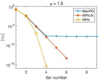
Figure 1: Comparisons with RPN and ManPG algorithms.

5.2 Local superlinear convergence of Algorithm 1

We proceed by testing the local superlinear convergence rate for different problem sizes in sparse PCA. For this task, we will use the polar retraction [AMS08, Example 4.1.3] defined as $R_{x}(\eta_{x})=(x+\eta_{x})(\operatorname{\mathrm{I}}_{r}+\eta_{x}^{\operatorname{\mathrm{T}}}\eta_{x})^{-1/2}$, where $x\in\mathrm{St}(n,r)$, $\eta_{x}\in\operatorname{\mathrm{T}}_{x}\mathrm{St}(n,r)$. We generate the random data matrix $A\in\operatorname{\mathbb{R}}^{m\times n}$ such that its entries are drawn from the standard normal distribution $\mathcal{N}(0,1)$. In Algorithm 1, we set $m=50$ and use $t=1/(2\|A\|_{2}^{2})$, which corresponds to the choice of the stepsize in [CMSZ20, HW22a].

In order to observe the local superlinear convergence, we first choose an initial point $x_{0}$ that is sufficiently close $x_{*}$, where $x_{*}$ is a stationary point of (1.1). Theorem 4.3 shows that $x_{k}$ is sufficiently close to $x_{*}$ when $v_{k}$ is sufficiently small, so we first run the ManPG algorithm to choose a point $x_{k}$ satisfying $\|v_{k}\|_{\operatorname{\mathrm{F}}}\leq 10^{-4}$ as the initial point $x_{0}$ of Algorithm 1. Figure 2 shows $\|v_{k}\|$ versus the number of iterations for multiple values of $n$, $r$, and $\mu$. We can see that the proposed method RPN empirically shows superlinear convergence results which is consistent with the theoretical result.

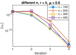
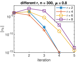
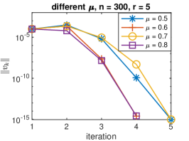
Figure 2: Random data: the norm of search direction for the SPCA. Top left: different $n=\{100,200,300,400\}$ with $r=5$ and $\mu=0.6$; Top right:different $r=\{2,4,6,8\}$ with $n=300$ and $\mu=0.8$; Bottom: different $\mu=\{0.5,0.6,0.7,0.8\}$ with $n=300$ and $r=5$

5.3 Comparisons with ManPG algorithm

In this section, we consider the version of sparse PCA with $r=1$, which admits a simple computation of $u_{k}$ by solving the linear equations (3.2). Thus (5.1) is simplified as

$$\min_{x\in\mathbb{S}^{n-1}}-x^{\operatorname{\mathrm{T}}}A^{\operatorname{\mathrm{T}}}Ax+\mu\|x\|_{1},$$ (5.4)

where the Stiefel manifold reduces to the unit sphere, as discussed in [JTU03, dGJL04]. We compare RPN-G, as stated in Algorithm 2, with the proximal Riemannian gradient method ManPG in [CMSZ20].

The parameters are set as those in Section 5.2. $\epsilon$ is set to be $10^{-4}$. Linear system (3.2) is solved by the built-in Matlab function cgs. ManPG does not terminate until the number of iterations attains the maximal iteration (3000). RPN-G does not terminate until $\|v_{k}\|\leq 10^{-12}$.

Random data:

The matrix $A$ is generated as that in Section 5.2. The results with multiple values of $n$ and $\mu$ are reported in Table 1 and Figure 4. Compared to ManPG, the proposed method RPN-G is able to obtain higher accurate solutions in the sense that $\|v_{k}\|$ from RPN-G is in double precision whereas that from ManPG is only in single precision. In addition, the number of Riemannian proximal Newton steps is not large and usually is only 5-6 iterations. It follows that the RPN-G is faster than ManPG when high accurate solution is needed, as shown in Figure 4.

Synthetic data:

The comparisons are repeated for synthetic data, which is generated by following the experiments in [HW22a, SCE⁺18]. Specifically, the five principal components shown in Figure 3 are repeated $m/5$ times to obtain $m\times n$ noise-free matrix. Then the data matrix $A$ is created by adding each entry of the noise-free matrix by i.i.d. random value drawn from $\mathcal{N}(0,0.25)$. We set $m=400$, $n=4000$ and $\mu=1.2$.

The left and right plots in Figure 5 show $\|v_{k}\|$ versus the number of iterations and $\|v_{k}\|$ versus CPU time, respectively. The behavior of RPN-G and ManPG on the synthetic data is similar to that on the random data, that is, RPN-G converges faster in the sense of both computational time and the number of iterations.

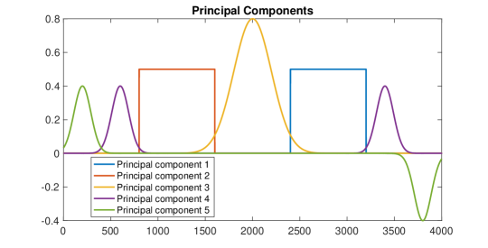
Figure 3: The five principal components used in the synthetic data.

Table 1: An average result of 5 random runs for random data with different setting of $(n,\mu)$. The subscript $k$ indicates a scale of $10^{k}$. iter-v denotes iterations to reach the optimal $\|v_{k}\|$ for the first time, for example, in the second row, 897 denotes the number of iterations that make $\|v_{k}\|$ firstly attain $10^{-8}$. iter-u denotes the number of using the new search direction $u_{k}$.

$(n,\mu)$	Algo	iter	iter-v	iter-u	$f$	sparsity	$\|v_{k}\|$
(5000,1.5)	ManPG	3000	897	-	$-4.59_{1}$	0.37	$7.41_{-8}$
(5000,1.5)	RPN-G	334	-	5	$-4.59_{1}$	0.37	$4.53_{-16}$
(10000,1.8)	ManPG	3000	1736	-	$-1.02_{2}$	0.32	$2.19_{-8}$
(10000,1.8)	RPN-G	580	-	6	$-1.02_{2}$	0.32	$5.69_{-16}$
(30000,2.0)	ManPG	3000	1283	-	$-3.98_{2}$	0.22	$1.19_{-8}$
(30000,2.0)	RPN-G	347	-	5	$-3.98_{2}$	0.22	$5.25_{-15}$
(50000,2.2)	ManPG	3000	1069	-	$-7.06_{2}$	0.18	$4.56_{-7}$
(50000,2.2)	RPN-G	789	-	5	$-7.06_{2}$	0.18	$1.41_{-14}$
(80000,2.5)	ManPG	3000	834	-	$-1.17_{3}$	0.17	$1.41_{-6}$
(80000,2.5)	RPN-G	839	-	6	$-1.17_{3}$	0.17	$1.94_{-15}$

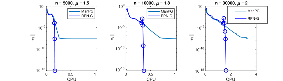
Figure 4: Random data: the norm of search direction $v_{k}$ versus CPU for different $(n,\mu)$, where the blue circle indicates the use of the new direction $u_{k}$.

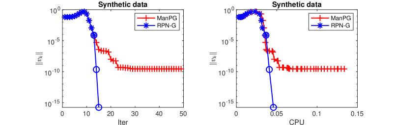
Figure 5: Plots of $\|v_{k}\|$ versus iterations and CPU times respectively, where $\|v_{k}\|$ is the norm of search direction, data matrix $A\in\operatorname{\mathbb{R}}^{4000\times 400}$ is from the synthetic data, $\mu$ is set to be 1.2. Note that the blue circle indicates the use of the new direction $u_{k}$.

Remark 5.2.

Here, we discuss the numbers of floating point arithmetic (flop) for computing $v_{k}$ and $u_{k}$ per iteration. For sparse PCA with $r=1$, the main computation cost is on $Ax$ and $A^{\operatorname{\mathrm{T}}}Ax$ for ManPG, and its flops is $\mathcal{O}(4mn)$, where $A\in\operatorname{\mathbb{R}}^{m\times n}$. Besides the computations in the function value and gradient evaluation, there are computations in the semismooth Newton iterations, where its dominant computational costs focus on $\Psi(\lambda)=B_{x_{k}}^{T}\left(\operatorname{\mathrm{prox}}_{th}\bigl{(}x_{k}-t\left[\nabla f(x_{k})+B_{x_{k}}\lambda\right]\bigr{)}-x_{k}\right)$ in (3.7) and

$$J_{\Psi}(\lambda_{k})[d]=B_{x_{k}}^{T}\left(\partial\operatorname{\mathrm{prox}}_{th}(x_{k}-t\left[\nabla f(x_{k})+B_{x_{k}}\lambda\right])\right)\circ\left(-tB_{x_{k}}d\right),$$

where $\circ$ denotes the entrywise product of two matrices. The computations of $\Psi(\lambda)$ and $J_{\Psi}(\lambda_{k})[d]$ in one evaluation are respectively $\mathcal{O}(4n)$ and $\mathcal{O}(6n)$. Thus, the total computation cost in the semismooth method is on the order of $\mathcal{O}(ssn_{k}*10n)$, where $ssn_{k}$ denotes the iteration number of semismooth Newton at $k$-th step. Therefore, the total complexity of ManPG in one evaluation is on the order of $\mathcal{O}(4mn+ssn_{k}*10n)$.

For RPN and RPN-G, we compute the direction $u_{k}$ by additionally solving $J(x_{k})[u_{k}]=-v_{k}$. We first compute $v_{k}$ by semismooth Newton method and its cost is also $\mathcal{O}(4mn+ssn_{k}*10n)$. When $u_{k}$ is solved by the built-in Matlab function $cgs$, the dominant computational cost per iteration comes from multiplying a vector by the matrix $J(x_{k})$. Assuming that $cgs$ takes $inner_{k}$ iterations for computing $u_{k}$, and the nonzero element of $x_{k}$ is $sp$, the computation of

$$J(x_{k})d= -d+M_{x_{k}}d-M_{x_{k}}x_{k}(x_{k}^{\operatorname{\mathrm{T}}}M_{x_{k}}x_{k})^{-1}x_{k}^{\operatorname{\mathrm{T}}}M_{x_{k}}d$$

$$-t(M_{x_{k}}-M_{x_{k}}x_{k}(x_{k}^{\operatorname{\mathrm{T}}}M_{x_{k}}x_{k})^{-1}x_{k}^{\operatorname{\mathrm{T}}}M_{x_{k}})*(-2A^{\operatorname{\mathrm{T}}}Ad+\lambda_{k}d)$$

costs $\mathcal{O}(2m(n+sp))$ flops. Thus, the overall computation of $u_{k}$ is $\mathcal{O}(inner_{k}*2m(n+sp)+4mn)$. Therefore, when the direction $u_{k}$ is computed, the total complexity of RPN and RPN-G in one evaluation is on the order of $\mathcal{O}(4mn+ssn_{k}*10n+inner_{k}*2m(n+sp))$. According to the numerical test, the inner iteration number for $cgs$ is usually 4 or 5 iterations.

6   Conclusion and Future Work

In this paper, we proposed a Riemannian proximal Newton method for solving optimization problems with separable structure, $f+\mu\|x\|_{1}$, over an embedded submanifold. It is proven that the proposed algorithm achieves superlinear convergence under certain reasonable assumptions. We further proposed a hybrid method that combines a Riemannian proximal gradient method and the Riemannian proximal Newton method. The hybrid method has been proven to have global convergence and the local superlinear convergence rate. Numerical results demonstrate the effectiveness of the proposed methods.

There are several directions for future research. In this paper, we have only considered a specific type of optimization problem, namely $f(x)+h(x)$ with $h(x)=\mu\|x\|_{1}$, on an embedded submanifold. It would be natural to extend the Riemannian proximal Newton method to handle more general nonsmooth functions $h(x)$ and more general manifolds. Additionally, we have only proposed a hybrid method for achieving global convergence, where the global convergence relies on the empirical selection of parameters. Therefore, it would be valuable to further investigate the globalization of the Riemannian proximal Newton method.

Appendix A Semismooth Implicit Function Theorem

The implicit function theorem for semismooth function comes from [Gow04, Theorem 4], it relies on the inverse function theorem for G-semismooth function [Gow04, Theorem 2], we first restate the result in Lemma A.1.

Lemma A.1 (G-semismooth Inverse Function Theorem).

Suppose that $f:\Omega\to\operatorname{\mathbb{R}}^{n}$ be G-semismooth function with respect to $\mathcal{K}_{f}$ on $\Omega$, where $\Omega\subset\operatorname{\mathbb{R}}^{n}$ be an open set. Fix a point $x^{0}\in\Omega$ and suppose that

• If $f$ is differentiable at $x\in\Omega$, then $\nabla f(x)\in\mathcal{K}_{f}(x)$.

• the multivalued mapping $x\mapsto\mathcal{K}_{f}(x)$ is compact valued and upper semicontinuous at each point of $\Omega$.

• $T_{f}(x^{0})$ consists of positively (negatively) oriented matrices.

• the topological index of $f$ at $x^{0}$ is 1 (respectively, -1), i.e., $\mathrm{index}(f,x^{0})=1$(respectively, -1).

Then there exists an open neighborhood $\mathcal{U}$ of $x^{0}$ and an open neighborhood $\mathcal{V}$ of $f(x^{0})$ such that $f:\mathcal{U}\to\mathcal{V}$ is bijective and $f$ has an inverse $h:\mathcal{V}\to\mathcal{U}$ that is locally Lipschitz, and $h$ is G-semismooth at each $v\in\mathcal{V}$ with respect to $\mathcal{K}_{h}(v)=\{A^{-1}:A\in\mathcal{K}_{f}(u)\}$ and $v=f(u)$, where the map $v\mapsto\mathcal{K}_{h}(v)$ is compact valued and upper semicontinuous at each point of $\mathcal{V}$.

Note that Lemma A.1 requires the notion of positively (negatively) oriented matrices and the notion of a topological index of a function. A matrix is said to be positively (negatively) oriented if it has a positive (negative) determinant sign. The topological index is, however, not easy to verify. Fortunately, a sufficient condition has been given in [PSS03, Theorem 6] and we give it in Lemma A.2.

Lemma A.2.

Let $\Phi:\mathbb{R}^{n}\to\mathbb{R}^{n}$ be Lipschitz continuous in an open neighborhood $\mathcal{D}$ of a vector $x^{0}$. Consider the following statements:

• every matrix in $\partial\Phi(x^{0})$ is nonsingular;

• for every $V\in\partial_{\mathrm{B}}\Phi(x^{0})$, $\mathrm{sgn}\det V=\mathrm{index}(\Phi,x^{0})=\pm 1$.

It holds that $(a)\Rightarrow(b)$.

We present and prove the semismooth implicit function theorem in Corollary A.3, which is a rearrangement of Lemma A.1 and Lemma A.2.

Corollary A.3 (Restatement of Corollary 2.7).

Suppose that $F:\mathbb{R}^{n}\times\mathbb{R}^{m}\to\mathbb{R}^{m}$ is a semismooth function with respect to $\partial_{\mathrm{B}}F$ in an open neighborhood of $(x^{0},y^{0})$ with $F(x^{0},y^{0})=0$. Let $H(y)=F(x^{0},y)$. If every matrix in $\partial H(y^{0})$ is nonsingular, then there exists an open set $\mathcal{V}\subset\mathbb{R}^{n}$ containing $x^{0}$, a set-valued function $\mathcal{K}:\mathcal{V}\rightrightarrows\mathbb{R}^{m\times n}$, and a G-semismooth function $f:\mathcal{V}\to\mathbb{R}^{m}$ with respect to $\mathcal{K}$ satisfying $f(x^{0})=y^{0}$,

$$F(x,f(x))=0$$

for every $x\in\mathcal{V}$ and the set-valued function $\mathcal{K}$ is

$$\mathcal{K}:x\mapsto\{-(A_{y})^{-1}A_{x}:[A_{x}\ A_{y}]\in\partial_{\mathrm{B}}F\big{(}x,f(x)\big{)}\},$$

where the map $x\mapsto\mathcal{K}(x)$ is compact valued and upper semicontinuous.

Proof.

Since every matrix in $\partial H(y^{0})$ is nonsingular, where $H:\operatorname{\mathbb{R}}^{m}\to\operatorname{\mathbb{R}}^{m}:y\mapsto H(y)=F(x^{0},y)$, then it follows Lemma A.2, for every $V\in\partial_{\mathrm{B}}H(x^{0})$, $\mathrm{sgn}\det V=\mathrm{index}(H,x^{0})=\pm 1$. Note that $H$ is also G-semismooth at $y^{0}$ with respect to

$$\mathcal{K}_{H}(y^{0})=\{A_{y}:[A_{x}\ A_{y}]\in\partial_{\mathrm{B}}F\big{(}x^{0},y^{0}\big{)}\},$$

where the map $y\mapsto\mathcal{K}_{H}(y)$ is compact valued and upper semicontinuous. Define $\mathcal{F}:\mathcal{D}\to\mathbb{R}^{n}\times\mathbb{R}^{m}$ by

$$\mathcal{F}(x,y)=\left(x,F(x,y)\right),$$

where $\mathcal{D}\subset\mathbb{R}^{n}\times\mathbb{R}^{m}$ is an open set including $(x^{0},y^{0})$. It is easily seen that $\mathcal{F}$ is G-semismooth at $(x^{0},y^{0})\in\mathcal{D}$ with respect to

$$\mathcal{K}_{\mathcal{F}}(x^{0},y^{0})=\{\begin{bmatrix}\operatorname{\mathrm{I}}_{n}&0\\ A_{x}&A_{y}\end{bmatrix}:[A_{x}\ A_{y}]\in\partial_{\mathrm{B}}F\big{(}x^{0},y^{0}\big{)}\},$$

where the map $(x,y)\mapsto\mathcal{K}_{\mathcal{F}}(x,y)$ is compact valued and upper semicontinuous.

We now verify conditions (i)-(iv) of Lemma A.1 for $\mathcal{F}$. Since $\mathcal{K}_{\mathcal{F}}(x,y)$ is defined with the $\partial_{\mathrm{B}}F\big{(}x,y\big{)}$, then conditions (i) and (ii) are clearly satisfied for $\mathcal{F}$ and $\mathcal{K}_{\mathcal{F}}$. As for conditions (iii) and (iv), it involves the property of topological index and the verification process of conditions (iii) and (iv) is exactly the same as that proof of [Gow04, Theorem 4], we omit it and refer interested reader to [Gow04] for more detail.

According to Lemma A.1, there exist a neighborhood $\mathcal{U}$ of $(x^{0},y^{0})$ and a neighborhood $\mathcal{V}\times\mathcal{W}$ of $\mathcal{F}(x^{0},y^{0})$ such that for every $v\in\mathcal{V}$ and $w\in\mathcal{W}$, there is a unique $z=(x,y)\in\mathcal{U}$ such that

$$\mathcal{F}(z)=(v,w).$$

Since $\mathcal{F}(x^{0},y^{0})=(x^{0},0)$, we can fix $\omega$ to be 0. Thus, for each $v\in\mathcal{V}$, there is a unique $z=(x,y)\in\mathcal{U}$ with

$$(x,F(x,y))=\mathcal{F}(z)=(v,0),$$

which implies that $x=v$ and $F(x,y)=0$. Thus, for every $x\in\mathcal{V}$, there is a unique $y$ such that $(x,y)\in\mathcal{U}$ and $F(x,y)=0$. Therefore, $y$ is the function of $x$, we let $y=f(x)$, where $x\in\mathcal{V}$, then $\mathcal{F}(x,f(x))=0$ for any $x\in\mathcal{V}$. Furthermore, let $\mathcal{H}:\mathcal{V}\times\mathcal{W}\to\mathcal{U}$ denote the inverse of $\mathcal{F}$ on $\mathcal{U}$. According to Lemma A.1, $\mathcal{H}$ is also G-semismoooth at any $(v,w)\in\mathcal{V}\times\mathcal{W}$ with respect to $\mathcal{K}_{\mathcal{H}}(v,w)=\{M^{-1}:M\in\mathcal{K}_{\mathcal{F}}(x,y)\}$, where $\mathcal{F}(x,y)=(v,w)$ and the map $(v,w)\mapsto\mathcal{K}_{\mathcal{H}}(v,w)$ is compacted valued and upper semicontinuous at each point of $\mathcal{V}\times\mathcal{W}$.

Now $f$ can be written as

$$f=\mathcal{P}_{2}\circ\mathcal{H}\circ\phi,$$

where $\phi$ is the inclusion map $\phi:\operatorname{\mathbb{R}}^{n}\to\operatorname{\mathbb{R}}^{n}\times\operatorname{\mathbb{R}}^{m}:x\mapsto\phi(x)=(x,0)$ and $\mathcal{P}_{2}$ is the projection map $\mathcal{P}_{2}:\operatorname{\mathbb{R}}^{n}\times\operatorname{\mathbb{R}}^{m}\to\operatorname{\mathbb{R}}^{m}:(x,y)\mapsto\mathcal{P}_{2}(x,y)=y$. Thus, $f$ is also G-semiismooth with respect to

$$\mathcal{K}(x) =\left\{\begin{bmatrix}0&\operatorname{\mathrm{I}}_{m}\end{bmatrix}\begin{bmatrix}\operatorname{\mathrm{I}}_{n}&0\\ A_{x}&A_{y}\end{bmatrix}^{-1}\begin{bmatrix}\operatorname{\mathrm{I}}_{n}\\ 0\end{bmatrix}:[A_{x}\ A_{y}]\in\partial_{\mathrm{B}}F\big{(}x,f(x)\big{)}.\right\}$$

$$=\{-(A_{y})^{-1}A_{x}:[A_{x}\ A_{y}]\in\partial_{\mathrm{B}}F\big{(}x,f(x)\big{)}\},$$

where the map $x\to\mathcal{K}(x)$ is compacted valued and upper semicontinuous.

∎

References

• [AGO20] H S Aghamiry, A Gholami, and S Operto. Full waveform inversion by proximal Newton method using adaptive regularization. Geophysical Journal International, 224(1):169–180, 09 2020.
• [AMS08] P.-A. Absil, R. Mahony, and R. Sepulchre. Optimization algorithms on matrix manifolds. Princeton University Press, Princeton, NJ, 2008.
• [AP16] Hedy Attouch and Juan Peypouquet. The rate of convergence of Nesterov’s accelerated forward-backward method is actually faster than $1/k^{2}$. SIAM Journal on Optimization, 26:1824–1834, 2016.
• [BAC19] Nicolas Boumal, P. A. Absil, and Coralia Cartis. Global rates of convergence for nonconvex optimization on manifolds. IMA Journal of Numerical Analysis, 39:1–33, 1 2019.
• [Bec17] Amir Beck. First-order methods in optimization. SIAM, 2017.
• [BESS19] Matthias Bollhöfer, Aryan Eftekhari, Simon Scheidegger, and Olaf Schenk. Large-scale sparse inverse covariance matrix estimation. SIAM Journal on Scientific Computing, 41:A380–A401, 2019.
• [Bou23] Nicolas Boumal. An introduction to optimization on smooth manifolds. Cambridge University Press, 2023.
• [BT09a] Amir Beck and Marc Teboulle. Fast gradient-based algorithms for constrained total variation image denoising and deblurring problems. IEEE Transactions on Image Processing, 18:2419–2434, 2009.
• [BT09b] Amir Beck and Marc Teboulle. A fast iterative shrinkage-thresholding algorithm for linear inverse problems. SIAM Journal on Imaging Sciences, 2:183–202, 2009.
• [Cla90] Frank H Clarke. Optimization and nonsmooth analysis. SIAM, 1990.
• [CMSZ20] Shixiang Chen, Shiqian Ma, Anthony Man-Cho So, and Tong Zhang. Proximal gradient method for nonsmooth optimization over the Stiefel manifold. SIAM Journal on Optimization, 30:210–239, 2020.
• [CSG+19] Haoran Chen, Yanfeng Sun, Junbin Gao, Yongli Hu, and Baocai Yin. Solving partial least squares regression via manifold optimization approaches. IEEE Transactions on Neural Networks and Learning Systems, 30:588–600, 2 2019.
• [dGJL04] Alexandre d’Aspremont, Laurent Ghaoui, Michael Jordan, and Gert Lanckriet. A direct formulation for sparse PCA using semidefinite programming. In Advances in Neural Information Processing Systems, volume 17. MIT Press, 2004.
• [DRR09] Asen L Dontchev, R Tyrrell Rockafellar, and R Tyrrell Rockafellar. Implicit functions and solution mappings: A view from variational analysis, volume 11. Springer, 2009.
• [FP03] Francisco Facchinei and Jong-Shi Pang. Finite-dimensional variational inequalities and complementarity problems. Springer, 2003.
• [Gow04] M. Seetharama Gowda. Inverse and implicit function theorems for H-differentiable and semismooth functions. Optimization Methods and Software, 19:443–461, 10 2004.
• [HAG17] Wen Huang, P. A. Absil, and K. A. Gallivan. Intrinsic representation of tangent vectors and vector transports on matrix manifolds. Numerische Mathematik, 136:523–543, 6 2017.
• [HHY18] S. Hosseini, W. Huang, and R. Yousefpour. Line search algorithms for locally Lipschitz functions on Riemannian manifolds. SIAM Journal on Optimization, 28:596–619, 2018.
• [HW22a] Wen Huang and Ke Wei. An extension of fast iterative shrinkage-thresholding algorithm to Riemannian optimization for sparse principal component analysis. Numerical Linear Algebra with Applications, 29, 1 2022.
• [HW22b] Wen Huang and Ke Wei. Riemannian proximal gradient methods. Mathematical Programming, 194:371–413, 7 2022.
• [HW23] Wen Huang and Ke Wei. An inexact Riemannian proximal gradient method. Computational Optimization and Applications, 2023.
• [HWGD22] Wen Huang, Meng Wei, Kyle A. Gallivan, and Paul Van Dooren. A Riemannian optimization approach to clustering problems, 2022.
• [Jos79a] Norman H Josephy. Newton’s method for generalized equations. Technical report, Wisconsin Univ-Madison Mathematics Research Center, 1979.
• [Jos79b] Norman H Josephy. Quasi-Newton methods for generalized equations. Technical report, Wisconsin Univ-madison Mathematics Research Center, 1979.
• [JTU03] Ian T. Jolliffe, Nickolay T. Trendafilov, and Mudassir Uddin. A modified principal component technique based on the lasso. Journal of Computational and Graphical Statistics, 12:531–547, 9 2003.
• [KP02] Steven George Krantz and Harold R Parks. The implicit function theorem: history, theory, and applications. Springer Science & Business Media, 2002.
• [KV17] Sahar Karimi and Stephen Vavasis. IMRO: A proximal quasi-Newton method for solving $\ell_{1}$-regularized least squares problems. SIAM Journal on Optimization, 27:583–615, 2017.
• [Lee18] John M Lee. Introduction to Riemannian manifolds, volume 2. Springer, 2018.
• [LL15] Huan Li and Zhouchen Lin. Accelerated proximal gradient methods for nonconvex programming. In Advances in Neural Information Processing Systems, 2015.
• [LSS14] Jason D. Lee, Yuekai Sun, and Michael A. Saunders. Proximal Newton-type methods for minimizing composite functions. SIAM Journal on Optimization, 24:1420–1443, 2014.
• [LST18] Xudong Li, Defeng Sun, and Kim Chuan Toh. On efficiently solving the subproblems of a level-set method for fused lasso problems. SIAM Journal on Optimization, 28:1842–1866, 2018.
• [LYL16] Canyi Lu, Shuicheng Yan, and Zhouchen Lin. Convex sparse spectral clustering: single-view to multi-view. IEEE Transactions on Image Processing, 25:2833–2843, 6 2016.
• [MYZZ23] Boris S. Mordukhovich, Xiaoming Yuan, Shangzhi Zeng, and Jin Zhang. A globally convergent proximal Newton-type method in nonsmooth convex optimization. Mathematical Programming, 198:899–936, 3 2023.
• [Nes83] Yurii Nesterov. A method for solving the convex programming problem with convergence rate $\mathcal{O}(1/k^{2})$. Proceedings of the USSR Academy of Sciences, 269:543–547, 1983.
• [Nes18] Yurii Nesterov. Lectures on convex optimization, volume 137. Springer, 2018.
• [OLCO13] Vidvuds Ozoliņš, Rongjie Lai, Russel Caflisch, and Stanley Osher. Compressed modes for variational problems in mathematics and physics. Proceedings of the National Academy of Sciences, 110:18368–18373, 11 2013.
• [PJL+13] Han Pan, Zhongliang Jing, Ming Lei, Rongli Liu, Bo Jin, and Canlong Zhang. A sparse proximal Newton splitting method for constrained image deblurring. Neurocomputing, 122:245–257, 12 2013.
• [PSS03] Jong-Shi Pang, Defeng Sun, and Jie Sun. Semismooth homeomorphisms and strong stability of semidefinite and Lorentz complementarity problems. Mathematics of Operations Research, 28(1):39–63, 2003.
• [PZ18] Seyoung Park and Hongyu Zhao. Spectral clustering based on learning similarity matrix. Bioinformatics, 34:2069–2076, 6 2018.
• [QS93] Liqun Qi and Jie Sun. A nonsmooth version of Newton’s method. Mathematical Programming, 58:353–367, 1993.
• [SCE+18] Karl Sjöstrand, Line Harder Clemmensen, Gudmundur Einarsson, Rasmus Larsen, and Bjarne Ersbøll. SpaSM: A MATLAB toolbox for sparse statistical modeling. Journal of Statistical Software, 84, 2018.
• [SSS18] P. J.S. Santos, P. S.M. Santos, and S. Scheimberg. A proximal Newton-type method for equilibrium problems. Optimization Letters, 12:997–1009, 7 2018.
• [Sun01] Defeng Sun. A further result on an implicit function theorem for locally Lipschitz functions. Operations Research Letters, 28:193–198, 2001.
• [SYGL14] Xiaoshuang Shi, Yujiu Yang, Zhenhua Guo, and Zhihui Lai. Face recognition by sparse discriminant analysis via joint $\ell_{2,1}$-norm minimization. Pattern Recognition, 47:2447–2453, 2014.
• [Tib96] Robert Tibshirani. Regression shrinkage and selection via the lasso. Journal of the Royal Statistical Society: Series B (Methodological), 58:267–288, 1 1996.
• [Ulb11] Michael Ulbrich. Semismooth Newton methods for variational inequalities and constrained optimization problems in function spaces. SIAM, 2011.
• [VSBV13] Silvia Villa, Saverio Salzo, Luca Baldassarre, and Alessandro Verri. Accelerated and inexact forward-backward algorithms. SIAM Journal on Optimization, 23:1607–1633, 2013.
• [WOR12] Christian Widmer, Cwidmer@cbio Mskcc Org, and Gunnar Rätsch. Multitask learning in computational biology. In Proceedings of ICML Workshop on Unsupervised and Transfer Learning, volume 27, pages 207–216. PMLR, 2012.
• [WY23] Qinsi Wang and Wei Hong Yang. Proximal quasi-Newton method for composite optimization over the Stiefel manifold. Journal of Scientific Computing, 95, 5 2023.
• [XLWZ18] Xiantao Xiao, Yongfeng Li, Zaiwen Wen, and Liwei Zhang. A regularized semismooth Newton method with projection steps for composite convex programs. Journal of Scientific Computing, 76:364–389, 7 2018.
• [ZHT06] Hui Zou, Trevor Hastie, and Robert Tibshirani. Sparse principal component analysis. Journal of Computational and Graphical Statistics, 15:265–286, 6 2006.
• [ZLwK+17] Yuqian Zhang, Yenson Lau, Han wen Kuo, Sky Cheung, Abhay Pasupathy, and John Wright. On the global geometry of sphere-constrained sparse blind deconvolution. In Proceedings of the IEEE Conference on Computer Vision and Pattern Recognition, pages 4894–4902, 2017.
• [ZX18] Hui Zou and Lingzhou Xue. A selective overview of sparse principal component analysis. Proceedings of the IEEE, 106:1311–1320, 8 2018.
• [ZYDR14] Kai Zhong, Ian E H Yen, Inderjit S Dhillon, and Pradeep Ravikumar. Proximal quasi-Newton for computationally intensive $\ell_{1}$-regularized $M$-estimators. In Advances in Neural Information Processing Systems, 2014.