Block-regularized $5\times 2$ Cross-validated McNemar’s Test for Comparing Two Classification Algorithms

Abstract

In the task of comparing two classification algorithms, the widely-used McNemar’s test aims to infer the presence of a significant difference between the error rates of the two classification algorithms. However, the power of the conventional McNemar’s test is usually unpromising because the hold-out (HO) method in the test merely uses a single train-validation split that usually produces a highly varied estimation of the error rates. In contrast, a cross-validation (CV) method repeats the HO method in multiple times and produces a stable estimation. Therefore, a CV method has a great advantage to improve the power of the McNemar’s test. Among all types of CV methods, a block-regularized $5\times 2$ CV (BCV) has been showed in many previous studies to be superior to the other CV methods in the comparison task of algorithms because the $5\times 2$ BCV can produce a high-quality estimator of the error rate by regularizing the numbers of overlapping records between all training sets. In this study, we compress the 10 correlated contingency tables in the $5\times 2$ BCV to form an effective contingency table. Then, we define a $5\times 2$ BCV McNemar’s test on the basis of the effective contingency table. We demonstrate the reasonable type I error and the promising power of the proposed $5\times 2$ BCV McNemar’s test on multiple simulation and real-world data sets.

1 Introduction

In machine learning domain, the popular McNemar’s test aims to compare the error rates of two classification algorithms and choose the better one. It has been widely applied in various real-world applications, including image classification [1, 2], speech and emotion recognition [3, 4], sentiment classification [5, 6], and word segmentation task [7].

The conventional McNemar’s test is typically conducted with a hold-out (HO) validation that merely uses a single train-validation split on a data set. The train set is used to train the two classification algorithms in a comparison, and the validation set is used to induce a $2\times 2$ contingency table that summarizes the counts of the inconsistent predictions between the two algorithms. Because the HO estimator of the error rate of an algorithm is usually unstable [8, 9, 10], the power of the conventional McNemar’s test is unpromising [11].

Compared with an HO validation, a cross-validation (CV) repeats HO validation in multiple times and averages all HO estimators to produce a more stable estimator of the error rate [12]. Therefore, a CV method has a great potential to improve the power of the McNemar’s test. In this study, we aim to improve the McNemar’s test with a CV method. Nevertheless, because all the HO validations in a CV method are performed on a single data set, the contingence tables and the McNemar’s test statistics induced from the multiple HO validations in a CV are correlated. Therefore, the main challenge in the construction of a CV-based McNemar’s test is how to aggregate the correlated contingency tables to form a reasonable McNemar’s test statistic.

An intuitive way to overcome the challenge is summing up all McNemar’s test statistics in a CV method. Specifically, considering the immensely popular $K$-fold CV [8, 13], the $K$ McNemar’s test statistics in a $K$-fold CV are naïvely assumed to be independent and summed up to form a novel test statistic following a $\chi^{2}$ distribution with $K$ degrees of freedom (DoF). However, because there is a large overlap between the $K$ training sets in a $K$-fold CV when $K>2$, the $K$ McNemar’s test statistics are correlated. Thus, the constructed test statistic are unreasonable. In this study, the intuitive McNemar’s test is named a naïve $K$-fold CV McNemar’s test, and it is not recommended.

Previous studies illustrated that a block-regularized $5\times 2$ CV (BCV) has more advantages than the $K$-fold CV in the task of algorithm comparison [14]. Specifically, Dietterich showed that the $5\times 2$ CV outperforms the $K$-fold CV in the paired $t$-tests for comparing classification algorithms [9]. Alpaydin further employed $5\times 2$ CV to develop a combined $F$-test [15]. Furthermore, Wang et al. developed a $3\times 2$ BCV $t$-test and showed that it has comparable type I error and power with the $5\times 2$ CV paired $t$-test and $F$-test [16]. Wang, Li, and Li developed a calibrated $F$-test based on a $5\times 2$ BCV [17], and it achieves the state-of-the-art performance in the task of algorithm comparison. In fact, a $5\times 2$ BCV regularizes the numbers of overlapping records between all training sets, and thus it enjoys a minimal variance property and induces a stable estimator of the error rate of an algorithm [14]. Therefore, we consider using a $5\times 2$ BCV to develop a novel McNemar’s test in this study.

Considering ten contingency tables in a $5\times 2$ BCV are correlated, instead of directly summing up the ten McNemar’s test statistics, we compress the ten correlated contingency tables into a virtual table named an effective contingency table through a reasonable Bayesian investigation where two correlation coefficients between estimators of the disagreement probability in the ten contingency tables are defined and analyzed. The effective contingency table helps us define a novel McNemar’s test analogous to the conventional McNemar’s test. Under a reasonable setting of the correlation coefficients, the novel McNemar’s test is named a $5\times 2$ BCV McNemar’s test.

Extensive experiments are conducted on multiple synthetic data sets and real-world data sets, involving several commonly used classification algorithms. Type I error and power curve are used to measure the performance of a significance test for a comparison of two classification algorithms. Moreover, 14 existing significance tests are investigated in the experiments. The experimental results illustrate that the proposed $5\times 2$ BCV McNemar’s test is superior to the other test methods.

The rest of the paper is organized as follows. We investigate the conventional McNemar’s test in Section 2. We then introduce a naïve $K$-fold CV McNemar’s test in Section 3. Our proposed $5\times 2$ BCV McNemar’s test is elaborated in Section 4. Our experiments and observations are reported in Section 5, followed by a conclusion in Section 6. Proofs of all theorems and lemmas are presented in Appendix.

2 Conventional McNemar’s Test

2.1 McNemar’s test on an HO validation

We let $D_{n}=\{z_{i}:z_{i}=(\boldsymbol{x}_{i},y_{i})\}_{i=1}^{n}$ be a data set consisting of $n$ iid records that are drawn from an unknown population $\mathfrak{D}$. In a record $z_{i}$, $\boldsymbol{x}_{i}$ is a predictor vector, and $y_{i}$ is the true class label of $\boldsymbol{x}_{i}$. We let $\mathcal{A}$ and $\mathcal{B}$ be the two classification algorithms that are compared on $D_{n}$. The comparison task is formalized into the following hypothesis testing problem:

$$H_{0}:\ \mu_{\mathcal{A}}-\mu_{\mathcal{B}}=0\ \ vs.\ \ H_{1}:\ \mu_{\mathcal{A}}-\mu_{\mathcal{B}}\neq 0,$$ (1)

where $\mu_{\mathcal{A}}$ and $\mu_{\mathcal{B}}$ are the error rates of $\mathcal{A}$ and $\mathcal{B}$, respectively, and they are also known as the generalization errors of $\mathcal{A}$ and $\mathcal{B}$ with the one-zero loss [18].

The problem in Eq. (1) can be addressed with a McNemar’s test. The conventional McNemar’s test is performed coupled with an HO validation. In an HO validation, $D_{n}$ is divided into two sub-blocks with a partition $(S,T)$ where $S$ and $T$ correspond to training and validation sets such that $S\cup T=D_{n}$ and $S\cap T=\emptyset$. The sizes of training and validation sets are $n_{1}=|S|$ and $n_{2}=|T|$, respectively.

On the basis of a partition $(S,T)$, algorithms $\mathcal{A}$ and $\mathcal{B}$ are trained on the training set $S$ and generate two classifiers, namely, $\mathcal{A}(S)$ and $\mathcal{B}(S)$. Then, the two classifiers are evaluated on the validation set $T$. The validation result can be summarized into a contingency table $\mathcal{C}=(n_{00},n_{01},n_{10},n_{11})$ such that $n_{00}+n_{01}+n_{10}+n_{11}=n_{2}$. Interpretation of $\mathcal{C}$ is given in Table I.

TABLE I: Interpretation of contingency table $\mathcal{C}$.

		Model $\mathcal{B}(S)$
		Incorrect	Correct
Model $\mathcal{A}(S)$	Incorrect	$n_{00}$: Count of records in $T$ misclassified by both $\mathcal{A}$ and $\mathcal{B}$.	$n_{01}$: Count of records in $T$ misclassified by $\mathcal{A}$ but not by $\mathcal{B}$.
	Correct	$n_{10}$: Count of records in $T$ misclassified by $\mathcal{B}$ but not by $\mathcal{A}$.	$n_{11}$: Count of records in $T$ misclassified by neither $\mathcal{A}$ nor $\mathcal{B}$.

On the basis of $\mathcal{C}$, the conventional McNemar’s test uses the following statistic [19]:

$$\mathcal{M}^{\textrm{HO}}=\frac{(|n_{01}-n_{10}|-1)^{2}}{n_{01}+n_{10}}\sim\chi^{2}(1),$$ (2)

where $-1$ in the numerator is a continuity correction [20]. If $\mathcal{M}^{\textrm{HO}}>\chi^{2}_{\alpha}(1)$ where $\alpha$ is the significance level, then $H_{0}$ is rejected.

2.2 Bayesian interpretation of $\mathcal{C}$

For a record $z$, let $y$ be the true class label, and let $\hat{y}_{\mathcal{A}}$ and $\hat{y}_{\mathcal{B}}$ be the predicted class labels of classifiers $\mathcal{A}(S)$ and $\mathcal{B}(S)$, respectively. Then, a contingency table $\mathcal{C}$ can be assumed to be a sample drawn from a multi-nomial distribution with parameters $\boldsymbol{\pi}=(\pi_{00},\pi_{01},\pi_{10},\pi_{11})$ such that $\pi_{00}+\pi_{01}+\pi_{10}+\pi_{11}=1$. Formally, we denote $\mathcal{C}|\boldsymbol{\pi}\sim\mathbf{M}(n_{2},\boldsymbol{\pi})$, or

$$P(\mathcal{C}|\boldsymbol{\pi})=\frac{n_{2}!}{n_{00}!n_{01}!n_{10}!n_{11}!}\pi_{00}^{n_{00}}\pi_{01}^{n_{01}}\pi_{10}^{n_{10}}\pi_{11}^{n_{11}},$$ (3)

where $\boldsymbol{\pi}$ is defined as follows:

$$\pi_{00} = P(\hat{y}_{\mathcal{A}}\neq y,\hat{y}_{\mathcal{B}}\neq y),$$

$$\pi_{01} = P(\hat{y}_{\mathcal{A}}\neq y,\hat{y}_{\mathcal{B}}=y),$$

$$\pi_{10} = P(\hat{y}_{\mathcal{A}}=y,\hat{y}_{\mathcal{B}}\neq y),$$

$$\pi_{11} = P(\hat{y}_{\mathcal{A}}=y,\hat{y}_{\mathcal{B}}=y).$$

From $\boldsymbol{\pi}$, several meaningful random variables are derived, including a disagreement probability $e$ and three conditional error rates $r$, $q_{a}$, and $q_{b}$. Correspondingly, the estimators of these random variables are induced from $\mathcal{C}$, namely, $E$, $R$, $Q_{a}$, and $Q_{b}$. Interpretation of these random variables and estimators are presented in Table II. Because $\mu_{\mathcal{A}}=\pi_{00}+\pi_{01}$ and $\mu_{\mathcal{B}}=\pi_{00}+\pi_{10}$, the problem in Eq. (1) can be rewritten as

$$H_{0}:\ r=0.5\ \ vs.\ \ H_{1}:\ r\neq 0.5.$$ (4)

TABLE II: Interpretation of several meaningful random variables defined on $\boldsymbol{\pi}$ and their estimators.

Notation	Definition	Probabilistic form	Estimator	Interpretation
$e$	$\pi_{01}+\pi_{10}$	$p(\hat{y}_{\mathcal{A}}\neq\hat{y}_{\mathcal{B}})$	$E=\frac{n_{01}+n_{10}}{n_{2}}$	Disagreement probability of the predictions between algorithms $\mathcal{A}$ and $\mathcal{B}$
$r$	$\frac{\pi_{01}}{\pi_{01}+\pi_{10}}$	$p(\hat{y}_{\mathcal{A}}\neq y|\hat{y}_{\mathcal{A}}\neq\hat{y}_{\mathcal{B}})$	$R=\frac{n_{01}}{n_{01}+n_{10}}$	Conditional error rate of algorithm $\mathcal{A}$ over the disagree predictions
$q_{a}$	$\frac{\pi_{01}}{\pi_{01}+\pi_{11}}$	$p(\hat{y}_{\mathcal{A}}\neq y|\hat{y}_{\mathcal{B}}=y)$	$Q_{a}=\frac{n_{01}}{n_{01}+n_{11}}$	Conditional error rate of algorithm $\mathcal{A}$ when algorithm $\mathcal{B}$ is correct
$q_{b}$	$\frac{\pi_{00}}{\pi_{10}+\pi_{00}}$	$p(\hat{y}_{\mathcal{A}}\neq y|\hat{y}_{\mathcal{B}}\neq y)$	$Q_{b}=\frac{n_{00}}{n_{10}+n_{00}}$	Conditional error rate of algorithm $\mathcal{A}$ when algorithm $\mathcal{B}$ is incorrect

In the estimators $E$, $R$, $Q_{a}$, and $Q_{b}$, the conditional distributions of $n_{01}+n_{10}$, $n_{00}$, and $n_{01}$ are as follows.

Lemma 1

Given that $\mathcal{C}|\boldsymbol{\pi}\sim\mathbf{M}(n_{2},\boldsymbol{\pi})$, we obtain

$$n_{01}+n_{10} \sim \mathbf{B}(n_{2},e),$$

$$n_{01}|n_{01}+n_{10} \sim \mathbf{B}(n_{01}+n_{10},r),$$

$$n_{01}|n_{01}+n_{11} \sim \mathbf{B}(n_{01}+n_{11},q_{a}),$$

$$n_{00}|n_{10}+n_{00} \sim \mathbf{B}(n_{01}+n_{00},q_{b}),$$

where $\mathbf{B}(\cdot,\cdot)$ represents a binomial distribution.

From a Bayesian perspective, priors of $e$, $r$, $q_{a}$, and $q_{b}$ are assumed to be a conjugate Beta distribution $Be(\lambda,\lambda)$. Therefore, the posterior distributions of $e$, $r$ $q_{a}$, and $q_{b}$ conditioned on $\mathcal{C}$ are presented in Lemma 2.

Lemma 2

With a Beta prior $Be(\lambda,\lambda)$, posterior distributions of $e$, $r$, $q_{a}$, and $q_{b}$ are

$$e|\mathcal{C} \sim Be(n_{01}+n_{10}+\lambda,n_{00}+n_{11}+\lambda),$$

$$r|\mathcal{C} \sim Be(n_{01}+\lambda,n_{10}+\lambda),$$

$$q_{a}|\mathcal{C} \sim Be(n_{01}+\lambda,n_{11}+\lambda),$$

$$q_{b}|\mathcal{C} \sim Be(n_{00}+\lambda,n_{10}+\lambda).$$

Corollary 1

Under the non-informative Beta prior with $\lambda=1$, the modes of the posteriors of $e$, $r$, $q_{a}$, and $q_{b}$ are

$$mode[e|\mathcal{C}] = E,$$

$$mode[r|\mathcal{C}] = R,$$

$$mode[q_{a}|\mathcal{C}] = Q_{a},$$

$$mode[q_{b}|\mathcal{C}] = Q_{b}.$$

It is noted that the Bayesian interpretation of a contingency table is not a main contribution of this study because a similar Bayesian interpretation of a confusion matrix has been developed for analyzing precision, recall, and $\textrm{F}_{1}$ score [21][22][23].

3 Naïve $K$-Fold CV McNemar’s Test

In this section, we introduce an intuitive way to integrate the McNemar’s test with a CV method. Considering the immensely popular $K$-fold CV, it produces $K$ contingency tables denoted as $\mathcal{C}_{k}=(n_{00,k},n_{01,k},n_{10,k},n_{11,k})$ with $k=1,\ldots,K$. Furthermore, according to Eq. (2), $K$ McNemar’s test statistics can be defined, namely, $\mathcal{M}^{\textrm{HO}}_{1},\ldots,\mathcal{M}^{\textrm{HO}}_{K}$. Furthermore, we sum up the $K$ statistics and construct the following statistic.

$$\mathcal{M}^{\textrm{KCV}}=\sum_{k=1}^{K}\mathcal{M}^{\textrm{HO}}_{k}=\sum_{k=1}^{K}\frac{(|n_{01,k}-n_{10,k}|-1)^{2}}{n_{01,k}+n_{10,k}}.$$ (5)

If $\mathcal{M}^{\textrm{HO}}_{1},\ldots,\mathcal{M}^{\textrm{HO}}_{K}$ are independent, then $\mathcal{M}^{\textrm{KCV}}\sim\chi^{2}(K)$. Therefore, if $\mathcal{M}^{\textrm{KCV}}>\chi^{2}_{\alpha}(K)$, then $H_{0}$ is rejected.

The above statistic is naïve because $\mathcal{M}_{1},\ldots,\mathcal{M}_{K}$ are correlated due to a large overlap between training sets in $K$-fold CV. Thus, $\mathcal{M}^{\textrm{KCV}}$ is not an exact $\chi^{2}(K)$. In this study, the test on $\mathcal{M}^{\textrm{KCV}}$ is named a naïve $K$-fold CV McNemar’s test, and it is not recommended.

4 $5\times 2$ BCV McNemar’s Test

4.1 $5\times 2$ BCV

Previous studies recommended a $5\times 2$ CV with random partitions (RCV) in a comparison of two algorithms [9][15][24]. However, the random partitions of a $5\times 2$ RCV probably lead to excessively overlapping training sets which would degrade the performance of a algorithm comparison method. In contrast, a $5\times 2$ BCV regularizes the numbers of overlapping records between any two training sets to be identical, and hence the variance of a $5\times 2$ BCV estimator of the error rate is smaller than that of a $5\times 2$ RCV estimator [14][17]. Therefore, a $5\times 2$ BCV provides a promising data partitioning schema for developing a novel algorithm comparison method.

Formally, a $5\times 2$ BCV performs five repetitions of two-fold CV partitioning with five regularized partitions. Let $\mathbb{P}=\{(S_{j},T_{j})\}_{j=1}^{5}$ denote a partition set of a $5\times 2$ BCV with regularized conditions of $|S_{j}|=|T_{j}|=n/2$ and $|S_{j}\cap S_{j^{\prime}}|\approx n/4$ for $j\neq j^{\prime}$. Each partition $(S_{j},T_{j})$ corresponds to a two-fold CV in which $S_{j}$ and $T_{j}$ are used as the training set in a round-robin manner.

For constructing $\mathbb{P}$, $D_{n}$ is first divided into eight equal-sized sub-blocks $D_{1},\ldots,D_{8}$. The sub-blocks are combined to form $\mathbb{P}$ with the heuristic rules in Table III that is extracted from the first five columns of a two-level orthogonal array $L_{8}(2^{7})$ in the domain of Design of Experiments (DoE) [25].

TABLE III: Partition set $\mathbb{P}$ of a $5\times 2$ BCV.

$j$	Fold $S$	Fold $T$
1	$D_{1},D_{2},D_{3},D_{4}$	$D_{5},D_{6},D_{7},D_{8}$
2	$D_{1},D_{3},D_{5},D_{7}$	$D_{2},D_{4},D_{6},D_{8}$
3	$D_{1},D_{2},D_{5},D_{6}$	$D_{3},D_{4},D_{7},D_{8}$
4	$D_{1},D_{4},D_{5},D_{8}$	$D_{2},D_{3},D_{6},D_{7}$
5	$D_{1},D_{3},D_{6},D_{8}$	$D_{2},D_{4},D_{5},D_{7}$

4.2 Contingency tables on $5\times 2$ BCV

When algorithms $\mathcal{A}$ and $\mathcal{B}$ are compared in a $5\times 2$ BCV, a collection of ten contingency tables is obtained, namely, $\boldsymbol{\mathcal{C}}_{5\times 2}=\{\boldsymbol{\mathcal{C}}^{(j)}\}_{j=1}^{5}=\{(\mathcal{C}_{1}^{(j)},\mathcal{C}_{2}^{(j)})\}_{j=1}^{5}$, where $\mathcal{C}_{k}^{(j)}=\left(n_{00,k}^{(j)},n_{01,k}^{(j)},n_{10,k}^{(j)},n_{11,k}^{(j)}\right)$ with $k=1,2$. Table $\mathcal{C}_{1}^{(j)}$ uses $S_{j}$ and $T_{j}$ as the training and validation sets. Table $\mathcal{C}_{2}^{(j)}$ uses $T_{j}$ and $S_{j}$ to train and validate an algorithm.

Furthermore, an averaged contingency table $\bar{\mathcal{C}}_{5\times 2}=(\bar{n}_{00},\bar{n}_{01},\bar{n}_{10},\bar{n}_{11})$ is obtained based on $\boldsymbol{\mathcal{C}}_{5\times 2}$, and it satisfies $\bar{n}_{00}+\bar{n}_{01}+\bar{n}_{10}+\bar{n}_{11}=n/2$ and

$$\bar{n}_{ii^{\prime}}=\frac{1}{10}\sum_{j=1}^{5}\sum_{k=1}^{2}n_{ii^{\prime},k}^{(j)},\ \ \ \ \forall i,i^{\prime}=0,1.$$ (6)

Correspondingly, the estimators of $e$, $r$, $q_{a}$, and $q_{b}$ in $\bar{\mathcal{C}}_{5\times 2}$ are defined as follows.

$$E_{5\times 2} = \frac{2(\bar{n}_{01}+\bar{n}_{10})}{n},$$

$$R_{5\times 2} = \frac{\bar{n}_{01}}{\bar{n}_{01}+\bar{n}_{10}},$$

$$Q_{a,5\times 2} = \frac{\bar{n}_{01}}{\bar{n}_{01}+\bar{n}_{11}},$$

$$Q_{b,5\times 2} = \frac{\bar{n}_{00}}{\bar{n}_{10}+\bar{n}_{00}}.$$

The denominator of $E_{5\times 2}$ is a constant, and thus

$$E_{5\times 2}=\sum_{j=1}^{5}\sum_{k=1}^{2}\frac{(n_{01,k}^{(j)}+n_{10,k}^{(j)})}{5n}=\sum_{j=1}^{5}\sum_{k=1}^{2}\frac{E_{k}^{(j)}}{10},$$ (7)

where $E_{k}^{(j)}$ is the estimator of $e$ on $\mathcal{C}_{k}^{(j)}$.

Theorem 1

The variance of $E_{5\times 2}$ is expressed as follows.

$$\textrm{Var}[E_{5\times 2}|e]=\frac{1+\rho_{1}+8\rho_{2}}{5n}e(1-e),$$ (8)

where $\rho_{1}$ and $\rho_{2}$ have the following definition.

• Let $\sigma^{2}=\textrm{Var}\left[E_{k}^{(j)}\right]=2e(1-e)/n$ be the variance of an HO estimator of $e$;

• $\rho_{1}=\textrm{Cov}\left[E_{1}^{(j)},E_{2}^{(j)}\right]/\sigma^{2}$ is the inter-group correlation coefficient of two HO estimators in $E^{(j)}$ in a two-fold CV.

• $\rho_{2}=\textrm{Cov}\left[E_{k}^{(j)},E_{k^{\prime}}^{(j^{\prime})}\right]/\sigma^{2}$ is the intra-group correlation coefficient of two HO estimators of $e$ in different two-fold CVs where $j\neq j^{\prime}$ and $k,k^{\prime}=1,2$.

Eq. (8) illustrates that $\rho_{2}$ plays a more important role than $\rho_{1}$. Moreover, because $\rho_{1}$ and $\rho_{2}$ have relations with specific algorithm types and data set distributions, it is hard to derive closed-form expressions of $\rho_{1}$ and $\rho_{2}$. Nevertheless, we are able to derive certain useful bounds of $\rho_{1}$ and $\rho_{2}$, and the bounds are indispensible in the statistical inference procedure in a comparison of two algorithms.

4.3 Properties of $\rho_{1}$ and $\rho_{2}$

Given that the five partitions in $5\times 2$ BCV are performed on a single data set, all $E_{k}^{(j)}$s on $\boldsymbol{\mathcal{C}}_{5\times 2}$ are correlated. Thus, $\rho_{1}$ and $\rho_{2}$ usually deviate from zero.

Several theoretical properties of $\rho_{1}$ and $\rho_{2}$ are elaborated as follows.

Lemma 3

Assume that $E_{k}^{(j)}$ merely depends on the validation set and $n$, then $\rho_{1}=0$ and $\rho_{2}=1/2$.

Nevertheless, the correlation between $E_{k}^{(j)}$s is also affected by the training sets in $5\times 2$ BCV because the training sets has a large overlap. Furthermore, under a mild assumption, the bound in Theorem 2 holds.

Theorem 2

Assume that $E_{k}^{(j)}$ depends on the data set size $n$, the validation set, and numbers of overlapping records between the training sets in a $5\times 2$ BCV, the correlation coefficients $\rho_{1}$ and $\rho_{2}$ satisfy the following bound.

$$\rho_{2}<(1+\rho_{1})/2.$$ (9)

Furthermore, if $\rho_{1}=0$, then $\rho_{2}<1/2$.

Many previous studies have investigated $\rho_{1}$ and $\rho_{2}$ over a broad family of loss functions, different algorithms, and various data sets [14][16][17]. These studies confirmed that the bound in Theorem 2 holds, and they showed the bound is loose. Furthermore, these studies slightly tighten the bound to the following form.

$$\rho_{1}\leq 1/2\ \ \textrm{and}\ \ 0\leq\rho_{2}\leq 1/2.$$ (10)

They further revealed that the tight bounds hold with a high probability. Thus, they recommended the bounds in Eq. (10) in a practical comparison scenario of two algorithms. Figure 1 also verifies that most values of $\rho_{1}$ and $\rho_{2}$ satisfy the bounds in Eq. (10).

4.4 Effective contingency table on a $5\times 2$ BCV

In this section, we introduce a notion of “effective contingency table” to approximate the posterior distributions of variables $e$, $r$, $q_{a}$, and $q_{b}$ conditioned on the ten correlated contingency tables in $\boldsymbol{\mathcal{C}}_{5\times 2}$. The effective contingency table is a single virtual contingency table that is denoted as $\mathcal{C}_{e}=(n_{00,e},n_{01,e},n_{10,e},n_{11,e})$. Moreover, let $n_{e}=n_{00,e}+n_{01,e}+n_{10,e}+n_{11,e}$ denote the effective validation set size of $\mathcal{C}_{e}$.

The estimators of $e$, $r$, $q_{a}$, and $q_{b}$ on $\mathcal{C}_{e}$ are defined as $E_{e}$, $R_{e}$, $Q_{a,e}$, and $Q_{b,e}$ with the following forms.

$$E_{e} = \frac{n_{01,e}+n_{10,e}}{n_{e}},$$

$$R_{e} = \frac{n_{01,e}}{n_{01,e}+n_{10,e}},$$

$$Q_{a,e} = \frac{n_{01,e}}{n_{01,e}+n_{11,e}},$$

$$Q_{b,e} = \frac{n_{00,e}}{n_{10,e}+n_{00,e}}.$$

Under certain constraints with regard to the modes of $e$, $r$, $q_{a}$, and $q_{b}$ conditioned on $\mathcal{C}_{e}$ and the variance of the estimator $E_{e}$, a closed-form expression of $\mathcal{C}_{e}$ is given as follows.

Theorem 3

With the non-informative Beta prior and under the constraints of

$$mode[e|\mathcal{C}_{e}] = E_{5\times 2},$$

$$mode[r|\mathcal{C}_{e}] = R_{5\times 2},$$

$$mode[q_{a}|\mathcal{C}_{e}] = Q_{a,5\times 2},$$

$$mode[q_{b}|\mathcal{C}_{e}] = Q_{b,5\times 2},$$

$$Var[E_{e}|e] = Var[E_{5\times 2}|e],$$

the closed-form expression of $\mathcal{C}_{e}$ is

$$\mathcal{C}_{e}=\frac{10}{1+\rho_{1}+8\rho_{2}}\bar{\mathcal{C}}_{5\times 2},$$ (11)

where $n_{00,e}$, $n_{01,e}$, $n_{10,e}$, and $n_{11,e}$ are

$$n_{ii^{\prime},e}=\frac{10\bar{n}_{ii^{\prime}}}{1+\rho_{1}+8\rho_{2}},\ \ \ \forall i,i^{\prime}=0,1.$$

In terms of Eq. (11), we obtain the effective validation set size is

$$n_{e}=\frac{5n}{1+\rho_{1}+8\rho_{2}}.$$ (12)

4.5 $5\times 2$ BCV McNemar’s test

Conditioned on $\mathcal{C}_{e}$ and $\rho_{1}$ and $\rho_{2}$, analogous to $\mathcal{M}^{\textrm{HO}}$ in Eq. (2), a chi-squared statistic is defined as follows.

$$\mathcal{M}^{\textrm{BCV}}_{\rho_{1},\rho_{2}}=\frac{(|n_{01,e}-n_{10,e}|-1)^{2}}{n_{01,e}+n_{10,e}}\sim\chi^{2}(1),$$ (13)

An equivalent form of $\mathcal{M}^{\textrm{BCV}}_{\rho_{1},\rho_{2}}$ is obtained by substituting Eq. (11) into Eq. (13).

$$\mathcal{M}^{\textrm{BCV}}_{t}=\frac{t(|\bar{n}_{01}-\bar{n}_{10}|-1/t)^{2}}{\bar{n}_{01}+\bar{n}_{10}}\sim\chi^{2}(1),$$ (14)

where $t=10/(1+\rho_{1}+8\rho_{2})$.

However, $\mathcal{M}_{t}^{\textrm{BCV}}$ contains an unknown parameter $t$, and thus it can not be used in a significance test. With an increasing $t$, the statistic $\mathcal{M}^{\textrm{BCV}}_{t}$ becomes large, and the McNemar’s test induced from $\mathcal{M}^{\textrm{BCV}}_{t}$ tends to be a liberal test that easily produces false positive conclusions. In contrast, according to the “conservative principle” in the task of algorithm comparison [18], a smaller value of $t$ is preferred. Because $t$ is a monotonic decreasing function with regard to $\rho_{1}$ and $\rho_{2}$. Considering the bounds in Eq. (10), we set $\rho_{1}=\rho_{2}=0.5$ and thus $t=20/11$. The following test statistic is obtained.

$$\mathcal{M}^{\textrm{BCV}}=\frac{20(|\bar{n}_{01}-\bar{n}_{10}|-11/20)^{2}}{11(\bar{n}_{01}+\bar{n}_{10})}\sim\chi^{2}(1),$$ (15)

In this study, $\mathcal{M}^{\textrm{BCV}}$ is named a $5\times 2$ BCV McNemar’s test statistic. Furthermore, the decision rule in a $5\times 2$ BCV McNemar’s test is: If $\mathcal{M}^{\textrm{BCV}}>\chi^{2}_{\alpha}(1)$, then $H_{0}$ is rejected. Moreover, $\alpha=0.05$ and $\chi^{2}_{0.05}(1)\approx 3.841$ are used.

5 Experimental Results and Analysis

To validate the superiority of the proposed $5\times 2$ BCV McNemar’s test, we formulate three research questions (RQs).

RQ1:

How are the correlation coefficients $\rho_{1}$ and $\rho_{2}$ in Eq. (8) distributed?

RQ2:

Is the $5\times 2$ BCV McNemar’s test better than the existing comparison methods of two classification algorithms?

RQ3:

How the block-regularized partition set of the $5\times 2$ BCV performs in the proposed $5\times 2$ BCV McNemar’s test?

For comparing two classification algorithms, the state-of-the-art methods mainly contain 4 families of 17 different significance tests. The existing tests and their recommended settings are as follows.

1. $t$-test family (9 tests).

   1. Repeated HO (RHO) paired $t$-test with 15 repeated HOs and $n_{1}=2n/3$ [9].

   2. $K$-fold CV paired $t$-test with $K=10$ [9].

   3. $5\times 2$ CV paired $t$-test [9].

   4. Corrected RHO $t$-test with $n_{1}=9n/10$ and 15 repeated HOs [18].

   5. Pseudo bootstrap test [18].

   6. Corrected pseudo bootstrap test [18].

   7. Corrected $10\times 10$ CV $t$-test [26].

   8. Combined $5\times 2$ CV $t$-test [24].

   9. Blocked $3\times 2$ CV $t$-test [16].

2. $F$-test family (2 tests)

   1. Combined $5\times 2$ CV $F$-test [15].

   2. Calibrated $5\times 2$ BCV $F$-test [17].

3. $Z$-test family (3 tests)

   1. Proportional test with $n_{1}=2n/3$ [9].

   2. Conservative $Z$-test [18].

   3. $K$-fold CV-CI $Z$-test with $K=10$ and “out” type of variance estimator [27].

4. McNemar’s test family (3 tests)

   1. Conventional HO McNemar’s test with $n_{1}=2n/3$ [9].

   2. $K$-fold CV Naïve McNemar’s test with $K=10$.

   3. $5\times 2$ BCV McNemar’s test.

We exclude the conservative $Z$-test, pseudo bootstrap test, and corrected pseudo bootstrap test in all experiments because Nadeau and Bengio found these three tests are less powerful and more expensive than the corrected RHO $t$-test [18].

5.1 Experiments for RQ1

To show the distribution of $\rho_{1}$ and $\rho_{2}$, 29 real-world UCI data sets and seven popular classification algorithms are used. All the real-world UCI data sets are listed in Table IV. For each data set, the record that contains missing values is omitted. The counts of records, predictors and classes in each data set are showed in Table IV. The seven classification algorithms used in the experiments are elaborated as follows.

1. Majority classifier. Test records are assigned with the class label with a maximum frequency in a training set. The assignment rule is independent to the input predictors.

2. Mean classifier. For each class, a mean vector of the predictors is calculated. A test record is assigned to the class whose mean vector has the smallest euclidean distance to the instance. It can be considered as a special case of linear discriminative analysis with a shared covariance matrix whose diagonals are equal and off-diagonals are zero.

3. logistic regression. The logistic regression classifier in “RWeka” package is used.

4. SVM. The support vector machine with sequential minimal optimization is considered. The “SMO” classifier with the default setting in “RWeka” package is used.

5. RIPPER. The “JRip” classifier with the default setting in “RWeka” package is used.

6. C4.5. The “J48” classifier with the default setting in “RWeka” package is used.

7. KNN. The k-nearest neighborhood classifier in “kknn” package is used. Parameter $k$ is set to 5, and a triangle kernel function is considered.

TABLE IV: Data sets used in the experiments in the submitted paper.

No.	Name	#Record	#Predictor	#Class
1	artificial	30654	7	10
2	australian	690	14	2
3	balance	625	4	3
4	car	1728	6	4
5	cmc	1473	9	3
6	credit	690	15	2
7	donors	748	4	2
8	flare	1388	10	2
9	german	1000	20	2
10	krvskp	3196	36	2
11	letter	20000	16	26
12	magic	19020	10	2
13	mammographic	830	5	2
14	nursery	12960	8	5
15	optdigits	5620	64	10
16	page_block	5473	10	5
17	pendigits	10992	16	10
18	pima	768	8	2
19	ringnorm	7400	20	2
20	satellite47	4435	36	6
21	spambase	4601	57	2
22	splice	3190	60	3
23	tic_tac_toe	958	9	2
24	titanic	2201	3	2
25	transfusion	748	4	2
26	twonorm	7400	20	2
27	wave	5000	40	3
28	wine_quality	4898	11	7
29	yeast	1484	7	10

On each data set, any two algorithms are compared, and thus $\binom{7}{2}=21$ different pairwise comparisons of algorithms are made. In total, $21\times 29=609$ experiments are conducted. In each experiment, we randomly sample 300 records from a data set without replacement and then perform the block-regularized partitions on the records and compute the estimations $E_{i}^{(j)}$. The process is repeated in 1,000 times. The values of $\rho_{1}$ and $\rho_{2}$ are obtained over the 1,000 repetitions.

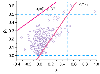
Figure 1: Scatter plot of $\rho_{1}$ and $\rho_{2}$.

Figure 1 shows the distribution of the numeric values of $\rho_{1}$ and $\rho_{2}$ over the 609 experiments. Three observations are obtained as follows.

1. Most values of $\rho_{1}$ and $\rho_{2}$ are distributed lower than 0.5. Moreover, $\rho_{1}$ varies around 0, and $\rho_{2}$ is greater than 0. Therefore, the bounds in Eq. (10) hold in a high probability. The observation is consistent to the previous studies.

2. All values of $\rho_{1}$ and $\rho_{2}$ are located at the right lower area of the red solid line $\rho_{2}=(1+\rho_{1})/2$. The observation confirms the bound in Theorem 2. Furthermore, there is a wide margin between the solid line and the scatter points, which indicates that the bound in Theorem 2 is loose.

3. Majority values of $\rho_{1}$ and $\rho_{2}$ satisfy $\rho_{2}\geq\rho_{1}$.

5.2 Experiments for RQ2

Three synthetic data sets and two real-world data sets are used to answer the RQ2.

Synthetic data set 1: Epsilon data set. The epsilon data set is developed by Dietterich [9] to investigate the type I error of a hypothesis test for comparing two classification algorithms. In the epsilon data set, on the basis of a data set size $n$, we directly generate the one-zero loss vectors of two algorithms. Specifically, let $i$ be a data record index where $i=1,\ldots,n$. Let $\mathbf{1}_{\mathcal{A}}(i)$ and $\mathbf{1}_{\mathcal{B}}(i)$ be the loss values of algorithms $\mathcal{A}$ and $\mathcal{B}$ on the $i$-th data record, respectively. Then, the loss values are generated according to the following rules.

• When $1\leq i\leq n/2$, $\mathbf{1}_{\mathcal{A}}(i)\sim\mathbf{B}(1,\epsilon/2)$ and $\mathbf{1}_{\mathcal{B}}(i)\sim\mathbf{B}(1,3\epsilon/2)$.

• When $n/2+1\leq i\leq n$, $\mathbf{1}_{\mathcal{A}}(i)\sim\mathbf{B}(1,3\epsilon/2)$ and $\mathbf{1}_{\mathcal{B}}(i)\sim\mathbf{B}(1,\epsilon/2)$.

According to the rules, we can obtain that on the first half of the data set, the error rates of algorithms $\mathcal{A}$ and $\mathcal{B}$ are $\mu_{\mathcal{A}}=\epsilon/2$ and $\mu_{\mathcal{A}}=3\epsilon/2$; on the remaining half of the data set, $\mu_{\mathcal{A}}=3\epsilon/2$ and $\mu_{\mathcal{A}}=\epsilon/2$; and on the entire data set, we obtain $\mu_{\mathcal{A}}=\mu_{\mathcal{B}}=\epsilon$, and thus the null hypothesis $H_{0}$ in Eq. (1) is true. Hence, the epsilon data set can merely be used to obtain the type I error of a test. In this data set, the settings of $n=300$ and $\epsilon=0.1$ are used.

Synthetic data set 2: EXP6 data set. The EXP6 data set is a six-class learning problem with two continuous predictors. It was developed in [28] and used in the algorithm comparison task in [9]. Specifically, in an EXP6 data set $D_{n}=\{(y_{i},\boldsymbol{x}_{i})\}_{i=1}^{n}$, let $\boldsymbol{x}=(x_{1},x_{2})$ be two predictors and $y$ be a true class label satisfying $y\in\{Y_{j}\}_{j=1}^{6}$. Predictors $x_{1}$ and $x_{2}$ in an EXP6 data set are uniformly distributed over an uniform grid space of resolution 0.1 over the region $\mathbf{X}=[0,15]\times[0,15]$. Class label $y_{\mathbf{x}}$ is generated as follows.

$$y_{\mathbf{x}}=\left\{\begin{aligned} Y_{1}&\ \ \ \ x_{2}-f_{1}(x_{1})\geq 0\ \land\ x_{2}-f_{2}(x_{1})\geq 0\\ Y_{2}&\ \ \ \ x_{2}-f_{1}(x_{1})<0\ \land\ x_{2}-f_{2}(x_{1})\geq 0\\ &\ \ \ \ \land\ x_{2}-f_{3}(x_{1})\geq 0\\ Y_{3}&\ \ \ \ x_{2}-f_{1}(x_{1})\geq 0\ \land\ x_{2}-f_{2}(x_{1})<0\\ Y_{4}&\ \ \ \ x_{2}-f_{1}(x_{1})<0\ \land\ x_{2}-f_{2}(x_{1})<0\\ &\ \ \ \ \land\ x_{2}-f_{3}(x_{1})\geq 0\\ Y_{5}&\ \ \ \ x_{2}-f_{2}(x_{1})\geq 0\ \land\ x_{2}-f_{3}(x_{1})<0\\ Y_{6}&\ \ \ \ x_{2}-f_{2}(x_{1})<0\ \land\ x_{2}-f_{3}(x_{1})<0\\ \end{aligned}\right.$$ (16)

where $f_{1}$, $f_{2}$ and $f_{3}$ are the following decision boundary functions.

$$f_{1}(x) = x^{2}-4x+6,$$

$$f_{2}(x) = 4sin(x/2)+8,$$

$$f_{3}(x) = -\frac{1}{25}(x^{2}-108x+236).$$ (17)

A scatter plot of an EXP6 data set with $n=300$ is showed in Figure 2. Furthermore, two algorithms are compared on an EXP6 data set.

It is a popular tree-based classification algorithm. J48 in package RWeka implements a C4.5 algorithm and is used with no pruning procedure.

First nearest neighbor uses a weighted Euclidean distance to tune its performance to the level of the C4.5. Specifically, the distance between points $\boldsymbol{x}_{i}=(x_{i1},x_{i2})$ and $\boldsymbol{x}_{j}=(x_{j1},x_{j2})$ is

$$d(\boldsymbol{x}_{i},\boldsymbol{x}_{j})=\omega(x_{i1}-x_{j1})^{2}+\omega^{-1}(x_{i2}-x_{j2})^{2},$$ (18)

where $\omega\in(0.0,1.0]$ is a tunable weight. When $\omega=1.0$, $d(\cdot,\cdot)$ degrades to the typical Euclidean distance.

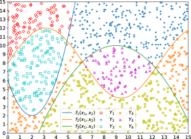
Figure 2: Demonstration of an EXP6 data set with $n=300$.

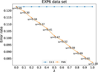
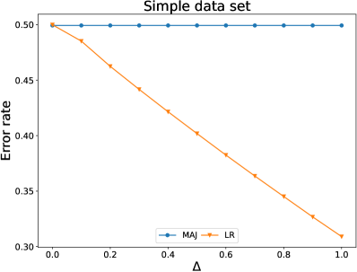
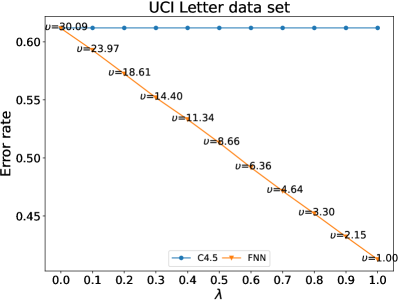
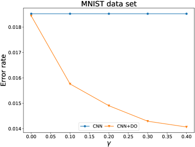
Figure 3: Simulations of true error rates of algorithms on the synthetic and real-world data sets

TABLE V: Type I errors of different algorithm comparison methods over synthetic and real-world data sets.

Family	Test	Synthetic			Real-world
		Epsilon	EXP6	Simple	UCI letter	MNIST
$t$-test family	RHO paired $t$-test	0.478	0.272	0.312	0.385	0.250
	$K$-fold CV paired $t$-test	0.043	0.076	0.109	0.142	0.090
	$5\times 2$ CV paired $t$-test	0.034	0.050	0.084	0.061	0.080
	Corrected RHO $t$-test	0.053	0.040	0.047	0.075	0.000
	Corrected $10\times 10$ CV $t$-test	0.035	0.040	0.063	0.082	0.080
	Combined $5\times 2$ CV $t$-test	0.291	0.156	0.214	0.236	0.150
	Blocked $3\times 2$ CV $t$-test	0.087	0.005	0.015	0.013	0.020
$F$-test family	Combined $5\times 2$ CV $F$-test	0.028	0.028	0.060	0.057	0.010
	Calibrated $5\times 2$ BCV $F$-test	0.035	0.025	0.055	0.042	0.040
$Z$-test family	Proportional test	0.056	0.016	0.014	0.054	0.020
	$K$-fold CV-CI $Z$-test	0.046	0.062	0.106	0.080	0.090
McNemar’s test family	Conventional HO McNemar’s test	0.031	0.037	0.029	0.062	0.060
	Naïve $K$-fold CV McNemar’s test	0.000	0.006	0.020	0.039	0.020
	$5\times 2$ BCV McNemar’s test	0.025	0.006	0.005	0.015	0.010

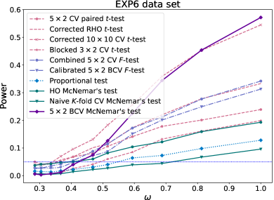
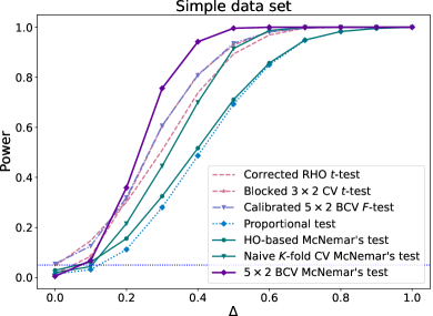
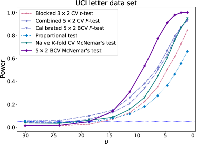
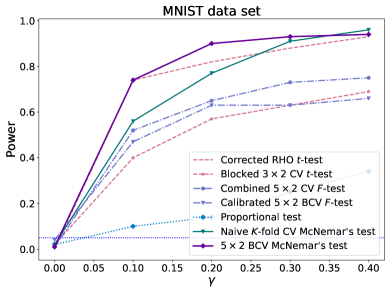
Figure 4: Power curves of different tests on the synthetic and real-world data sets.

True values of the error rates of C4.5 and FNN, namely, $\mu_{C4.5}$ and $\mu_{FNN,\omega}$, are obtained through taking averages over all estimates of the error rates of the classifiers that are trained over 1,000 iid EXP6 data sets with $n=300$ and evaluated with a large EXP6 data set with $(15/0.1+1)^{2}=22,801$ records. Because the error rate of FNN depends on the hyper-parameter $\omega$, we introduce multiple target error rates for FNN algorithm. Specifically, a target error rate $\mu_{target}$ is expressed as a linear interpolation value between $\mu_{C4.5}$ and $\mu_{FNN,1.0}$, i.e., $\mu_{target}=\mu_{C4.5}-\lambda(\mu_{C4.5}-\mu_{FNN,1.0})$. We adjust $\omega$ so that the true error rate of an FNN achieves $\mu_{target}$. The discrete values of $\lambda$ are derived from the range of [0.0, 1.0] with a step of 0.1. In particular, when $\lambda=0.0$, the target error rate of an FNN degrades to $\mu_{C4.5}$, which makes the null hypothesis $H_{0}$ in Eq. (1) being true.

Figure 3 shows the true error rate of C4.5 and FNN with various target error rates. Several specific observations are obtained from Figure 3. The true error rate of C4.5 is 12.27%. The true error rate of FNN decreases with an increasing $\omega$. When $\omega=1.0$, the error rate of FNN is 8.21%. When $\omega=0.29$, FNN achieves an identical error rate with C4.5. Therefore, type I error of a significance test method is obtained with the setting of $\omega=0.29$. Power curve of a test is depicted by increasing $\omega$ from 0.29 to 1.0.

Synthetic data set 3: Simple data set. Let $D_{n}=\{(x_{i},y_{i})\}_{i=1}^{n}$ be a simple binary classification data set where $y_{i}\in\{Y_{0},Y_{1}\}$ is the true class label and $x_{i}$ is the predictor. Class label index $i\sim\mathbf{B}(1,0.5)$ is independently drawn. Then, $x_{i}|y_{i}=Y_{1}\sim N(0,1)$ and $x_{i}|y_{i}=Y_{2}\sim N(\Delta,1)$ where $\Delta\in[0.0,1.0]$ is a tunable parameter. Moreover, on a simple data set, two algorithms are compared.

Logistic regression is implemented by the “glm” package in R software with a binomial link function.

Majority classifier uses the most frequent class label in the training set as a prediction that is independent to the input predictors.

True error rates of LR and MAJ on a simple data set are illustrated in Figure 3. Regardless of $\Delta$, the error rate of MAJ remains unchanged because it merely depends on the prior distribution of class labels. Moreover, when $\Delta=0.0$, the distributions of the predictor $x$ in two classes are completely overlapping, and thus LR degrades to a random guess that possesses an identical error rate with MAJ. When $\Delta$ increases, the error rate of LR monotonically decreases. Therefore, $\Delta=0.0$ is used to obtain the type I error of a test, and a power curve is depicted by increasing $\Delta$ from 0.0 to 1.0. In a simple data set, $n=1,000$ is used.

Real-world data set 1: UCI letter data set. It is a popular data set in the task of algorithm comparison [9, 18]. It contains 20,000 data points, 26 classes, and 16 predictors. The following two classification algorithms are compared.

Classification tree uses the package “tree” with default settings in R software.

First nearest neighbor uses a distorted distance $d(\cdot,\cdot)$ as follows [18].

$$d(\boldsymbol{x}_{i},\boldsymbol{x}_{j})=\sum_{k=1}^{3}\upsilon^{2-k}\sum_{l\in C_{k}}(x_{il}-x_{jl})^{2},$$ (19)

where $\boldsymbol{x}_{i}$ and $\boldsymbol{x}_{j}$ are two predictor vectors, $C_{1}=\{1,3,9,16\}$, $C_{2}=\{2,4,6,7,8,10,12,14,15\}$, and $C_{3}=\{5,11,13\}$. $\upsilon\in[1,50]$ is a tunable parameter to adjust the error rate of an FNN.

Furthermore, 1,000 data sets of $n=300$ are iid drawn from the letter data set with replacement. True values of the error rates of TREE and FNN are obtained by training the algorithms on the 1,000 data sets and validating on the entire letter data set. Similar to the EXP6 data set, the simulation of the true error rates is based on several targeted error rates characterized with an interpolation parameter $\lambda$. The true error rates are showed in Figure 3 which illustrates that the error rate of FNN monotonically increases with an increasing $\upsilon$. When $\upsilon=30.09$, FNN owns an identical error rate with TREE. Thus, the type I error of a test is obtained when $\upsilon=30.09$, and the power curve of a test is depicted by decreasingly changing $\upsilon$ from $30.09$ to $1.0$.

Real-world data set 2: MNIST data set. It is a popular ten-class classification data set in deep learning studies. The gold split of the MNIST data set in the keras library consists of a training set with 60,000 images and a test set with 10,000 images. We merely use the 60,000 images in the training set as a data population. Two deep learning models are compared.

The architecture of the used CNN is expressed as conv$\to$max_pooling$\to$conv$\to$max_pooling$\to$flatten $\to$dense$\to$softmax. We use ReLU as an activation function and cross-entropy as an objective function. The batch size and epoch count are set to 128 and 250. Numbers of filters in the two “conv” layers are 32 and 64, respectively. A same kernel size of $(5,5)$ is used in the two “conv” layers. Moreover, a pooling size of $(2,2)$ is used. Size of the hidden dense layer is 500, and size of the softmax layer is 10.

We apply dropout regularization to the weights between the flatten layer and the dense layer of the above CNN. The dropout rate $\gamma\in[0.0,1.0)$ is used to tune the error rate of CNN+DO.

Considering that it is computationally expensive to train a CNN model, we only generate 100 data sets, each of size $n=10,000$, to simulate 100 separate trails. We use the entire population as a test set to compute the true error rates by averaging the 100 estimators of the models trained on the 100 data set. We changes the drop out rate from 0.0 to 0.4 with a step of 0.1. The true values of the error rates of CNN and CNN+DO are plotted in the last plot of Figure 3. The true error rate of CNN is 1.85% regardless of dropout rate $\gamma$. The true error rate of CNN+DO is decreasing with an increasing drop out rate $\gamma$. When $\gamma=0.0$, the error rate of CNN+DO is equivalent to that of CNN. When $\gamma$ increases, CNN+DO has a lower error rate than CNN. Therefore, for a significance test, we use $\gamma=0.0$ obtain its type I error, and we obtain its power curve by changing $\gamma$ from 0.0 to 0.4.

The type I errors of all significance tests over the simulated and real-world data sets are presented in Table V. The type I errors below $\alpha=0.05$ is indicated in bold font. Two observations are obtained.

1. All type I errors of the $5\times 2$ BCV McNemar’s test and naïve $K$-fold CV McNemar’s test are lower than 0.05. It indicates that the two tests can effectively reduce false positive conclusions for algorithm comparison. Majority of type I errors of blocked $3\times 2$ CV $t$-test and calibrated $5\times 2$ BCV $F$-test are reasonable. In contrast, although $K$-fold CV paired $t$-test and $K$-fold CV-CI $Z$-test own reasonable type I errors on the epsilon data set, all type I errors of the two tests on other data sets exceed 0.05. Therefore, the two tests are unpromising for comparing two classification algorithms. Moreover, all type I errors of the RHO paired $t$-test, combined $5\times 2$ CV $t$-test are larger than 0.05, and thus the two tests which tend to produce false positive conclusions should be used with a very carefully manner in a practical scenario.

2. Over the five data sets, our proposed $5\times 2$ BCV McNemar’s test almost achieves the smallest type I errors which are obviously smaller than 0.05. Therefore, the $5\times 2$ BCV McNemar’s test is more conservative than the other tests because the bounds of $\rho_{1}$ and $\rho_{2}$ in Eq. (10) are loose. Therefore, how to refine the bounds of $\rho_{1}$ and $\rho_{2}$ to further improve a McNemar’s test is an important future research direction.

Figure 4 illustrates the power curves of the tests which own reasonable type I errors on the experimental data sets. A common conclusion obtained from all the plots in Figure 4 is that the $5\times 2$ BCV McNemar’s test possesses a more skewed power curve than the other tests. The observation indicates that the $5\times 2$ BCV McNemar’s test is the most powerful one among all the tests for comparing two classification algorithms.

In sum, all the experimental results in this section show that the $5\times 2$ BCV McNemar’s test possesses not only a reasonably small type I error but also a promising power. Thus, the $5\times 2$ BCV McNemar’s test is superior to the other tests and can reduce false positive conclusions in the task of algorithm comparison. Therefore, we recommend the $5\times 2$ BCV McNemar’s test in the practical comparison task of two classification algorithms.

5.3 Experiments for RQ3

We perform an ablation experiment to verify the effectiveness of the block-regularized partition set in the proposed $5\times 2$ BCV McNemar’s test. In the experiment, we substitute a $5\times 2$ BCV with a common $5\times 2$ RCV [9] with a random partition set. A $5\times 2$ RCV owns $\binom{5}{2}=10$ random numbers of overlapping records between any two training sets attributing to the randomness in a partition set. A number of overlapping records that deviates far from $n/4$ would lead to a low quality partition set [9][29]. If a number of overlapping records reach $n/2$, then two partitions in the partition set are identical. Nevertheless, it is hard to simultaneously control all the overlapping counts in a fine-grained manner and to gradually generate a low quality partition set. Therefore, in the experiment, we consider a family of particular partition sets that a $5\times 2$ RCV has a probability to produce through repeating a single partition in multiple times. Hence, the quality of a partition set in the family can be measured with the repetition count of a partition (RCP). If RCP equals zero, then all partitions are different. In contrast, if RCP is four, all partitions are identical and the partition set is the worst.

In the ablation experiment, considering the space limitation and computational cost, we concentrate on the UCI letter data set which is a popular data set in the studies of algorithm comparison [18][30]. Settings of the data set and algorithms are similar with those in Section 5.2. We compare a $5\times 2$ BCV and a $5\times 2$ RCV with different levels of RCP in a McNemar’s test in terms of the measures of type I error and power curve, respectively.

TABLE VI: Illustration of type I error and $\textrm{Var}[E_{e}]$ in the comparison of $5\times 2$ BCV and $5\times 2$ RCV on a McNemar’s test.

		Type I error	$\textrm{Var}[E_{e}]$
			$\upsilon=30.09$	$\upsilon=4.64$
$5\times 2$ BCV		0.013	3.486$\times 10^{-4}$	3.609$\times 10^{-4}$
$5\times 2$ RCV	RCP=0	0.020	3.724$\times 10^{-4}$	3.757$\times 10^{-4}$
	RCP=1	0.030	4.236$\times 10^{-4}$	4.397$\times 10^{-4}$
	RCP=2	0.033	5.453$\times 10^{-4}$	5.433$\times 10^{-4}$
	RCP=3	0.064	7.230$\times 10^{-4}$	7.078$\times 10^{-4}$
	RCP=4	0.106	9.364$\times 10^{-4}$	9.562$\times 10^{-4}$

Table VI shows type I errors of the McNemar’s tests with $5\times 2$ BCV and $5\times 2$ RCV. The $5\times 2$ BCV McNemar’s test owns the smallest type I error. In contrast, a $5\times 2$ RCV has a larger type I error than the $5\times 2$ BCV. The type I error of a $5\times 2$ RCV gradually increases with an increasing RCP. In particular, when RCP is greater than two, the type I error with a $5\times 2$ RCV exceeds the significance level $\alpha=0.05$. The observation indicates that type I error of a McNemar’s test has a close relationship with the quality of a random partition set. With an increasing RCP, the quality of the partition set of a $5\times 2$ RCV degrades, and the corresponding McNemar’s test tends to produce more false positive conclusions in a comparison of two classification algorithms.

Moreover, Table VI provides numerical values of $\textrm{Var}[E_{e}]$ under 1,000 simulations with $\upsilon=30.09$ (no difference between FNN and TREE) and $\upsilon=4.64$, respectively. In actual, $\textrm{Var}[E_{e}]$ is a key factor of an effective contingency table illustrated in Theorem 3. A more stable estimator $E_{e}$ would result in a better effective contingency table. From Table VI, we obtain that a $5\times 2$ BCV possesses an optimal property of the smallest variance of $E_{e}$. The variance of $E_{e}$ in a $5\times 2$ RCV is larger that that in $5\times 2$ BCV, and the variance increases when an RCP changes from 0 to 4. In another word, the estimator $E_{e}$ becomes unstable in a $5\times 2$ RCV that may degrade the performance of a McNemar’s test.

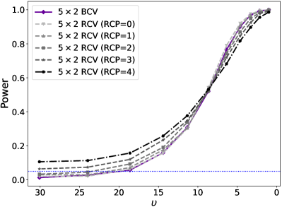
Figure 5: Illustration of the effect of low quality partitions of $5\times 2$ RCV on the McNemar’s test.

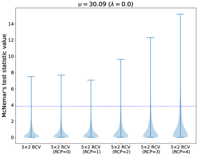
Figure 6: Violin plots of McNemar’s test statistic values in a comparison of $5\times 2$ BCV and $5\times 2$ RCV.

Figure 5 illustrates the effect of the quality of a partition set in a $5\times 2$ RCV on the power of a McNemar’s test. In Figure 5, when RCP increases, the McNemar’s test not only tends to produce more false positive conclusions ($\upsilon=30.09$), but also has a low power to distinguish the difference between the error rates of FNN and TREE. The latter observation is obtained from the figure in the range of $\upsilon\leq 6$. In contrast, $5\times 2$ BCV keeps a promising power in Figure 5. Therefore, from the perspective of power, a $5\times 2$ BCV should be preferred for constructing a novel McNemar’s test rather than a $5\times 2$ RCV.

To further investigate the power of a McNemar’s test, Figure 6 employs violin plots to show the distributions of numerical values of a McNemar’s test statistic in Eq. (15) with $\upsilon=30.09$ and $\upsilon=4.64$, respectively. The blue dotted horizontal line indicates $\chi^{2}_{0.05}(1)\approx 3.841$. When $\upsilon=30.09$, the error rates of FNN and TREE on the UCI letter data set are identical. From Figure 6, we obtain that in a $5\times 2$ RCV, when an RCP increases, the distribution of a McNemar’s test statistic spreads widely, and thus the McNemar’s test becomes unstable. In the first plot, when $\upsilon=30.09$, with an increasing RCP, the area of the distribution of a McNemar’s test statistic above the blue horizontal line becomes large, and thus more false positive conclusions are produced. In the second plot, when $\upsilon=4.64$, when an RCP increases, the area of the distribution under the blue horizontal line enlarges which indicates the power of the McNemar’s test is reducing. In contrast, $5\times 2$ BCV has a narrow distribution, and thus it achieves a promising performance in our proposed McNemar’s test.

6 Conclusion

In this study, we proposed a $5\times 2$ BCV McNemar’s test for comparing two classification algorithms. The proposed test is formulated based on a notion of “effective contingency table” that effectively compress the ten correlated contingency tables in a $5\times 2$ BCV with a Bayesian perspective. The correlations between the tables are well investigated, and theoretical bounds of the correlations are proved. Extensive experiments illustrate that the $5\times 2$ BCV McNemar’s test has a reasonable type I error and a promising power compared with the existing algorithm comparison methods.

In the future, we will refine the McNemar’s test in an $m\times 2$ BCV with a sequential setting and further investigate the $m\times 2$ BCV McNemar’s test from a Bayesian perspective for inferring informative decisions in the task of comparing classification algorithms.

References

- [1] J. d. Leeuw, H. Jia, L. Yang, X. Liu, K. S. Schmidt, and A. K. Skidmore, “Comparing accuracy assessments to infer superiority of image classification methods,” international journal of remote sensing, vol. 27, no. 1, pp. 223–232, 2006.
- [2] T. J. Brinker, A. Hekler, A. H. Enk, C. Berking, S. Haferkamp, A. Hauschild, M. Weichenthal, J. Klode, D. Schadendorf, T. Holland-Letz, C. v. Kalle, S. Fröhling, B. Schilling, and J. S. Utikal, “Deep neural networks are superior to dermatologists in melanoma image classification,” european journal of cancer, vol. 119, pp. 11–17, 2019.
- [3] L. Gillick and S. J. Cox, “Some statistical issues in the comparison of speech recognition algorithms,” in International Conference on Acoustics, Speech, and Signal Processing, 1989, Conference Proceedings, pp. 532–535 vol.1.
- [4] C. E. Erdem, E. Bozkurt, E. Erzin, and A. T. Erdem, “RANSAC-based training data selection for emotion recognition from spontaneous speech,” in Proceedings of the 3rd international workshop on Affective interaction in natural environments. ACM Press, 2010. [Online]. Available: https://doi.org/10.1145%2F1877826.1877831
- [5] L. Williams, C. Bannister, M. Arribas-Ayllon, A. Preece, and I. Spasić, “The role of idioms in sentiment analysis,” expert systems with applications, vol. 42, no. 21, pp. 7375–7385, 2015.
- [6] N. Mukhtar, M. A. Khan, and N. Chiragh, “Effective use of evaluation measures for the validation of best classifier in urdu sentiment analysis,” Cognitive Computation, vol. 9, no. 4, pp. 446–456, 2017. [Online]. Available: https://doi.org/10.1007/s12559-017-9481-5
- [7] Y. Sun, T. S. Butler, A. Shafarenko, R. Adams, M. Loomes, and N. Davey, “Word segmentation of handwritten text using supervised classification techniques,” Applied Soft Computing, vol. 7, no. 1, pp. 71–88, 2007.
- [8] R. Kohavi, “A study of cross-validation and bootstrap for accuracy estimation and model selection,” in Ijcai, vol. 14, 1995, Conference Proceedings, pp. 1137–1145.
- [9] T. G. Dietterich, “Approximate statistical tests for comparing supervised classification learning algorithms,” Neural computation, vol. 10, no. 7, pp. 1895–1923, 1998. [Online]. Available: http://www.mitpressjournals.org/doi/abs/10.1162/089976698300017197
- [10] J. D. Rodríguez, A. Pérez, and J. A. Lozano, “A general framework for the statistical analysis of the sources of variance for classification error estimators,” Pattern Recognition, vol. 46, no. 3, pp. 855–864, 2013. [Online]. Available: http://ac.els-cdn.com/S0031320312003998/1-s2.0-S0031320312003998-main.pdf?_tid=f45b1bfe-3ad1-11e7-b6c0-00000aacb35e&acdnat=1495006088_8c4c1e24a44a58088ac3b782ea57d4f6
- [11] M. Keller, S. Bengio, and S. Y. Wong, “Benchmarking non-parametric statistical tests,” in Advances in neural information processing systems, 2006, Conference Proceedings, pp. 651–658.
- [12] J. Friedman, T. Hastie, and R. Tibshirani, The elements of statistical learning. Springer series in statistics Springer, Berlin, 2001, vol. 1.
- [13] J. D. Rodríguez, A. Pérez, and J. A. Lozano, “Sensitivity analysis of k-fold cross validation in prediction error estimation,” IEEE Transactions on Pattern Analysis and Machine Intelligence, vol. 32, no. 3, pp. 569–575, 2010.
- [14] R. Wang, Y. Wang, J. Li, and X. Yang, “Block-regularized m2 cross-validated estimator of the generalization error,” Neural Computation, vol. 29, no. 2, pp. 519–554, 2017.
- [15] E. Alpaydin, “Combined 52 cv f test for comparing supervised classification learning algorithms,” Neural computation, vol. 11, no. 8, pp. 1885–1892, 1999.
- [16] Y. Wang, R. Wang, H. Jia, and J. Li, “Blocked 32 cross-validated t-test for comparing supervised classification learning algorithms,” Neural Computation, vol. 26, no. 1, pp. 208–235, 2014. [Online]. Available: http://dblp.uni-trier.de/db/journals/neco/neco26.html#WangWJL14
- [17] Y. Wang, J. Li, and Y. Li, “Choosing between two classification learning algorithms based on calibrated balanced cross-validated f-test,” Neural Processing Letters, vol. 46, no. 1, pp. 1–13, 2017. [Online]. Available: https://doi.org/10.1007/s11063-016-9569-z
- [18] C. Nadeau and Y. Bengio, “Inference for the generalization error,” Machine Learning, vol. 52, no. 3, pp. 239–281, 2003.
- [19] Q. McNemar, “Note on the sampling error of the difference between correlated proportions or percentages,” psychometrika, vol. 12, no. 2, pp. 153–157, 1947.
- [20] B. S. Everitt, The analysis of contingency tables. CRC Press, 1992.
- [21] C. Goutte and E. Gaussier, “A probabilistic interpretation of precision, recall and f-score, with implication for evaluation,” in Advances in Information Retrieval, D. E. Losada and J. M. Fernández-Luna, Eds. Berlin, Heidelberg: Springer Berlin Heidelberg, 2005, pp. 345–359.
- [22] Y. Wang and J. Li, “Credible intervals for precision and recall based on a k-fold cross-validated beta distribution,” Neural computation, vol. 28, no. 8, pp. 1694–1722, 2016.
- [23] R. Wang and J. Li, “Bayes test of precision, recall, and f1 measure for comparison of two natural language processing models,” in Proceedings of the 57th Annual Meeting of the Association for Computational Linguistics, 2019, pp. 4135–4145.
- [24] O. T. Yildiz, “Omnivariate rule induction using a novel pairwise statistical test,” Knowledge and Data Engineering, IEEE Transactions on, vol. 25, no. 9, pp. 2105–2118, 2013.
- [25] C. J. Wu and M. S. Hamada, Experiments: planning, analysis, and optimization. John Wiley & Sons, 2011, vol. 552.
- [26] R. R. Bouckaert and E. Frank, Evaluating the replicability of significance tests for comparing learning algorithms. Springer, 2004, pp. 3–12.
- [27] P. Bayle, A. Bayle, L. Janson, and L. Mackey, “Cross-validation confidence intervals for test error,” in Advances in Neural Information Processing Systems, vol. 33, 2020.
- [28] E. B. Kong and T. G. Dietterich, “Error-correcting output coding corrects bias and variance,” in ICML’95 Proceedings of the Twelfth International Conference on International Conference on Machine Learning, 1995, pp. 313–321.
- [29] R. Wang, J. Li, X. Yang, and J. Yang, “Block-regularized repeated learning-testing for estimating generalization error,” Information Sciences, vol. 477, pp. 246–264, 2019.
- [30] Y. Bengio and Y. Grandvalet, “No unbiased estimator of the variance of k-fold cross-validation,” J. Mach. Learn. Res., vol. 5, pp. 1089–1105, 2004.