Continual Learning for LiDAR Semantic Segmentation:
Class-Incremental and Coarse-to-Fine strategies on Sparse Data

Abstract

During the last few years, Continual Learning (CL) strategies for image classification and segmentation have been widely investigated designing innovative solutions to tackle catastrophic forgetting, like knowledge distillation and self-inpainting. However, the application of continual learning paradigms to point clouds is still unexplored and investigation is required, especially using architectures that capture the sparsity and uneven distribution of LiDAR data. The current paper analyzes the problem of class incremental learning applied to point cloud semantic segmentation, comparing approaches and state-of-the-art architectures. To the best of our knowledge, this is the first example of class-incremental continual learning for LiDAR point cloud semantic segmentation. Different CL strategies were adapted to LiDAR point clouds and tested, tackling both classic fine-tuning scenarios and the Coarse-to-Fine learning paradigm. The framework has been evaluated through two different architectures on SemanticKITTI [2, 16], obtaining results in line with state-of-the-art CL strategies and standard offline learning.

1 Introduction

The recent development of autonomous driving, equipped with automatic visual understanding systems, has fostered the research on object identification and segmentation towards more generalizable and portable strategies via inline learning behaviors in place of distinct offline training phases. Particularly, continual learning investigates the capability of incorporating new knowledge in well-established models, shifting to new tasks, labels, or data distributions. Indeed, most of the cases do not benefit from previous training data, which are unavailable due to portability, privacy issues, or costly labeling process. The process is thus usually accomplished by preserving previous knowledge, whilst avoiding catastrophic forgetting. Different CL strategies have been deeply investigated for classification [11, 24, 29, 43] and object detection [45, 23, 40] tasks, while less examples exist for semantic segmentation. The reason is that semantic segmentation is a harder task with respect to classification: classification is about providing one single class label for each image, while in segmentation already-known and totally-new classes can be present together in the same acquisition (image, point cloud, etc.). As a matter of fact, handling with such heterogeneity is one of the additional issues that is addressed considering multiple continual learning scenarios for semantic segmentation [36, 25, 13, 6, 48]. So far, continual learning has generally been applied to images in vision tasks. With respect to point cloud data, images are far simpler data to be retrieved, labeled, and processed thanks to their regular distribution in space, limited memory requirements, and computational cost. Instead, CL techniques on point cloud data are still quite unexplored, made an exception for a few attempts [5, 30, 12, 26, 8], and the investigation of class-incremental CL has not been considered yet. Even if it may seem a simple adaptation of image-based network architectures to point cloud, the sparsity of LiDAR point cloud data and the significant difference in the processing architectures makes their investigation anew. More precisely, the problem turns out to be more challenging in relation to point-based architectures [41, 42, 21], where raw points are directly processed with no discretization (see Sec. 2 for more details). In addition, the inherent nature of point cloud datasets, acquired with different methodologies and in different noise conditions, can vary the final accuracy.

This paper analyzes the challenges of class-incremental continual learning on point cloud semantic segmentation and adapts different CL solutions to different architectures and partitionings. The main novelties brought by this work can be listed as follows.

• It is the first application of class-incremental continual learning to LiDAR semantic segmentation, where point sparsity enhances the issues concerning the co-occurrence of already-known and totally-new classes.

• It provides a general evaluation of different techniques to mitigate catastrophic forgetting on LiDAR point clouds (adapted from image semantic segmentation to a domain with new peculiarities).

• It considers both general Class-Incremental and Coarse-to-Fine scenarios [28, 50, 34, 46].

The paper is structured as follows. Section 2 overviews recent state-of-the-art works, Section 3 presents the main single-headed class-incremental continual learning scenarios. Section 4 analyzes different CL solutions overviewing different partitioning and strategies to mitigate catastrophic forgetting. Finally, in Section 5 we discuss the results obtained with different techniques with a comparison among dataset setups and CL strategies; conclusions are drawn in Section 6.

2 Related Work

LiDAR Semantic Segmentation is usually tackled via deep learning solutions that treat input points in several ways: discretizing into voxels, projecting on 2D images, or processing directly as they are [3, 15]. Voxel based methods [47, 33] are generally used for well-structured point clouds (e.g., terrestrial laser scanning acquisitions [1]) and can easily apply 3D convolutions. Projection based methods [38, 51, 10] are well suited for LiDAR point clouds, as they are acquired in concentric circles and can be easily projected onto cylindrical [51] or spherical [38] surfaces. Both categories of methods are efficient in terms of computational complexity, but approximate point distributions to regular structures. Methods that directly process data [41, 42, 21] avoid such loss of structural information, which is crucial when dealing with few data samples and limited resources. Recent works rely on 4D convolutions [14] or transformers [18] to accomplish the task but require huge computational power and storage capacity; more lightweight approaches process points in mixed strategies, providing voxel-wise predictions refined with point-wise labels [53, 52]. Such models have been widely adopted for various learning approaches including class-balancing regularization [4, 10] Knowledge distillation [20] and open-world 3D scene understanding [5]. Some works have also adopted incremental learning settings for 3D data in object detection [12], place recognition [26], remote sensing [30] and few-shot learning [8]. Nonetheless, no prior work has explored Class-Incremental Continual Learning for LiDAR Semantic Segmentation.

Class-Incremental Continual Learning (CL) has developed a growing research interest for image classification [11, 24, 29, 43], object detection [45, 23, 40] tasks. Many of these works observed the catastrophic interference problem when sequentially learning examples of different input patterns. Among the most popular strategies to reduce forgetting are replay methods [43, 32] that store exemplars to be replayed in future steps and non-exemplar methods; among these parameter isolation dedicates different model parameters to each task to prevent any possible forgetting and regularization methods [29, 24, 48, 7], which add extra regularization loss to consolidate knowledge on previous data. This line of work avoids storing raw inputs, prioritizing privacy, and alleviating memory requirements.

CL in Semantic Segmentation literature is more limited [36, 25, 13, 6, 48]. Major attention has been devoted to class incremental semantic segmentation to learn new categories from new data. The problem is formalized in [36] and tackled with regularization approaches such as parameters freezing and knowledge distillation. In [25] knowledge distillation is coupled with a class importance weighting scheme to emphasize gradients on difficult classes. In [37] the latent space is regularized to improve class-conditional features separation. Cermelli et al. study the distribution shift of the background class in [7] and tackle the problem in a weakly-supervised fashion in [6]. Maracani et al. [32] proposed replaying old classes using either generative networks or web crawled images.

Coarse-to-Fine Semantic Segmentation has been explored in few previous work for part-based regularization [28, 50] and approaches where coarse-level classes are refined into finer categories [34, 46]. Previous approaches developed also different ways to draw class hierarchies. In [44] they are estimated a prior based on semantics; in [4], they are drawn a posteriori based on network misclassifications. Some examples have shown also developing Coarse-to-Fine for continual learning [44, 49], but no previous literature has explored with point cloud data.

	Training Subset $T_{0}$	Training Subset $T_{1}$	Training Subset $T_{2}$	Validation Set
	SemanticKITTI train			SemanticKITTI val
Sequences	$D_{0}=${01,02,03}	$D_{1}=${04,05,09,10}	$D_{2}=${00,06,07}	$D=${08}
Labeled classes	$C_{0}=$ {road, parking, sidewalk, other-ground, vegetation, terrain}	$C_{1}=$ {building, fence, trunk, pole, traffic-sign}	$C_{2}=$ {bicycle, motorcycle, truck, other-vehicle, person, bicyclist, motorcyclist, car}	$C=\{C_{0}\cup C_{1}\cup C_{2}\}$
# Clouds	$6563$	$4623$	$4541$	$4071$
# Points	$355280$	$375140$	$121494$	$19130$
% Labeled pt.	$81.73$%	$19.21$%	$8.82$%	$95.53\%$

Table 1: SemanticKITTI [2] subdivision in experiences. Training set classes and sequences are divided in three parts according to points frequency and cardinality, whilst following [25]. Underline denotes classes that are not present in Cityscapes [9], thus in the original partition.

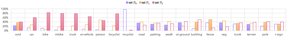
Figure 1: Histogram of point clouds percentage within each training dataset split $D_{k}$. The percentage is normalized for each class $c$ on the total number of points for that specific class in the whole dataset $D_{0}\cup D_{1}\cup D_{2}$.

3 Problem Formulation

Given an input point cloud, i.e., a set of $N$ 3D points ${\bf X}=\{{\bf x}_{1},{\bf x}_{2},\dots,{\bf x}_{N}\}$, and a set of candidate semantic labels $Y=\it\{y_{1},y_{2},\dots,y_{N}\}$, the objective of semantic segmentation is to associate each input point ${\bf x}_{i}$ with a semantic label $y_{i}$. Each label belongs to a given subset of semantic classes $C$ that contains also a special class $b$ (void, which corresponds to the background for images). The void class typically identifies objects out of the range of LiDAR precision or belonging to unknown classes. For the sake of clarity, we call it background as for images to avoid confusion with empty voxels and masked points. Semantic segmentation task is usually achieved by using a suitable deep learning model $\mathcal{M}:X\mapsto\hat{Y}_{C}$, commonly composed of a feature extractor $\mathcal{E}$ followed by a decoding module $\mathcal{D}$, $\mathcal{M}=\mathcal{D}\circ\mathcal{E}$.

In standard supervised learning, the model is learned in a single shot with standard offline training over a fixed and complete set of data $T\subset X\times Y$.

In class incremental learning, instead, we assume that the training is performed in multiple steps and only a subset of the training data is available for training at each step $k=0,\dots,K$. More in detail, we start from an initial step $k=0$ where only training data concerning a subset of all the classes $C_{0}\subset C$ is available (we assume that $b\in C_{0}$). We denote with $\mathcal{M}_{0}:X\mapsto\hat{Y}_{C_{0}}$, $\mathcal{M}_{0}=\mathcal{D}_{0}\circ\mathcal{E}_{0}$ the model trained after this initial step. At a generic step $k$, a new set of classes $C_{k}$ is added to the class collection $C_{0\rightarrow(k-1)}$ learned up to that point, resulting in an expanded set of learnable classes $C_{0\rightarrow k}=C_{0\rightarrow(k-1)}\cup C_{k}$ (we assume $C_{0\rightarrow(k-1)}\cap C_{k}=\emptyset$). The model after the $k$-th step of training is $\mathcal{M}_{k}:X\mapsto\hat{Y}_{C_{0\rightarrow k}}$, where $\mathcal{M}_{k}=\mathcal{D}_{k}\circ\mathcal{E}_{k}$.
Some approaches train the decoder alone after the initial step while keeping the encoder frozen. In our approach, both the encoder and decoder are updated, while only the last layer is changed. This is because the encoder is usually kept frozen when the training is performed on random objects datasets, and the proportion of data between the first step and the subsequent ones is unbalanced toward the first. Instead, in our partitioning (and in general, in autonomous driving datasets), dataset cardinality, number of samples, and frequency of classes are balanced across the different steps.

3.1 Scenarios

Multiple scenarios have been proposed for CL on image semantic segmentation[35, 36]. In each scenario, the original dataset $T$ is divided into $K$ groups that correspond to learning steps; the overall set of labels is also generally divided into $K$ groups. At learning step $k$, the training procedure updates the model using only the tuple $(T_{k},C_{k})$.

Sequential: samples in the $k$-th experience are provided with the labels of all the groups $\leq k$, while points with labels $>k$ are not present at all. Each learning step contains a unique set of samples, whose points belong to classes seen either in the current or in the previous steps.

Sequential masked: samples in the $k$-th experience are provided with the $k$-th experience labels, while the points with labels of classes $<k$ are marked as unlabeled, and points with labels $>k$ are not present at all. In this setup, each learning step contains a unique set of samples, whose points belong either to novel classes or to the unlabeled class, which is not predicted by the model and is masked out from both the results and the training procedure.

Disjoint: samples in the $k$-th experience are provided with the $k$-th experience labels, while points with labels of classes $<k$ are marked as background, and points with labels $>k$ are not present at all. At each learning step, the unique set of training samples is identical to the sequential setup, but old classes are gathered into a common label (background, instead of being unlabelled as in the Sequential masked scenario) that changes its distribution at each step.

Overlapped: At each learning step $k$ all the dataset samples are available but only the current step classes $C_{k}$ are labeled with the correct label and the rest ($C_{j}\neq C_{i}$) with the background labels, either if they belong to experience $j<k$ or $j>k$. In this setup, each training step contains all the point clouds that have at least one point belonging to a class in set $C_{k}$, with only the classes of the set annotated and the rest set to background. In this paper, this scenario is reported for comparison assuming that data can never be shared among different experiences.

Coarse-to-Fine: At each learning step $k$, all points are labeled but their classes are refined with respect to the previous step. At step $k$, coarse labels $C_{k-1}$ are substituted with labels from fine classes $C_{k},|C_{k}|>|C_{k-1}|$. Each coarse class corresponds to its unique set of fine classes.

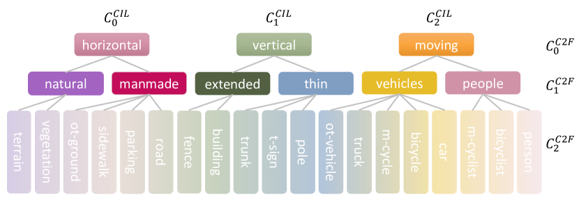
Figure 2: Class hierarchies in SemanticKITTI C2F partition. Each Coarse class is made-up by grouping classes belonging to the same learning step in CIL partition. Sequence splits $D_{k}$ are considered in the same identical order.

4 Methodology

We considered RandLA-Net [21], one of the most famous point-based architectures as a reference, in order to frame the problem in a perspective different from images (i.e., using MLPs in place of convolutional setting). RandLA-Net is an efficient point-based lightweight network composed of an MLP based encoder-decoder structure that achieves remarkably high efficiency in terms of memory and computation. In addition, we evaluate on Cylinder3D [53, 52] voxel based architecture for comparison. Nonetheless, the framework can be applied on top of any architecture for point cloud semantic segmentation.

SemanticKITTI [2, 16] has been chosen as a reference dataset, since it is one of the most popular benchmarks for LiDAR semantic segmentation in autonomous driving. SemanticKITTI consists of $43,552$ densely annotated LiDAR scans, $19,130$ for training, and $4,071$ for validating (that we used for testing, as done by all competing works being the test labels not publicly available).

4.1 Dataset Partitioning

We divided the dataset in order to define incremental experiences for continual learning. As no previous works can be found, we propose two subdivisions of SemanticKITTI: one based on class cardinality and frequency within different sequential acquisitions, and another based on a Coarse-to-Fine semantic partitioning. We denote the former as CIL, as it is based on the effective subdivision of [25], and the latter as C2F.

4.1.1 Semantic Partition (CIL)

Tab. 1 shows the first partition of SemanticKITTI, based on class cardinality and frequency within different sequential acquisitions. This grouping is based on the effective subdivision of Cityscapes [9] proposed in [25]. Cityscapes is an autonomous driving dataset for image semantic segmentation with a class set similar to SemanticKITTI. Specifically, in $T_{0}$ class sky is substituted with parking and other-ground, in $T_{1}$ traffic-light and walls with trunk, and in $T_{2}$ train, bus and rider are replaced with motorcyclist, bicylist and other-vehicle. Such classes are underlined in Tab. 1. Sequence subdivisions are chosen to maximize labeled classes in each group while keeping semantic consistency and balancing the total amount of points/acquisitions within each training subset. Fig. 1 shows the percentage of labeled points within each group normalized for each class $c$ on the cardinality of the specific class.

4.1.2 Coarse-to-Fine Partition (C2F)

Fig. 2 shows the second partition of SemanticKITTI, where grouping is made by splitting labels into three learning steps, and labels are clustered to guarantee semantic consistency. The first coarse set resembles the semantics of CIL: classes of each $C_{k}^{CIL}$ form a single coarse class in $C_{0}^{C2F}$. $C_{1}^{C2F}$ is obtained by further partitioning coarse classes into 2 mid-level classes each; finally, the fine set $C_{2}^{C2F}=C$, i.e., contains all the classes of SemanticKITTI. Note that this partition shares the dataset split of sequences with CIL setup reported in Tab 1.

4.2 CL Strategies

In standard training, background points are usually masked out from the learning procedure and the model weights are optimized using the cross-entropy objective

$$\mathcal{L}_{ce}=-\frac{1}{|T_{k}|}\sum_{{\rm\bf X}_{n}\in T_{k}}\sum_{c\in C_{k-1}}{\rm\bf Y}_{n}[c]\cdot\log(\mathcal{M}_{k}({\rm\bf X}_{n})[c])$$ (1)

where ${\rm\bf Y}_{n}[c]$ the one-hot encoded ground truth and $\mathcal{M}_{k}({\rm\bf X}_{n})[c]$ is the prediction score for class $c$. In the incremental learning setup, we assume that at each incremental training step $k$ only samples from new classes $C_{k}$ are available. In order to include this new information in the model, weights are initialized from previous model $\mathcal{M}_{k-1}$ ($k\geq 1$) and the new class set $C_{0\rightarrow k}$ is then learned by optimizing the standard objective $\mathcal{L}_{ce}(\mathcal{M}_{k};C_{0\rightarrow k},T_{k})$ with data from the current training partition $T_{k}$. However, a naïve fine tuning on novel classes leads to catastrophic forgetting, and therefore, by including points from past classes (no labels) as background, we can recover previous knowledge by self-predicting old labels. To this extent, we consider two strategies: Knowledge Distillation (KD) [29] and Background Self-Inpainting [32]. Fig. 3 provides a visual summary of these techniques.

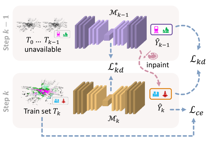
Figure 3: Summary of continual learning strategies employed. At the current learning step ($k$) only training set $T_{k}$ and previous model $\mathcal{M}_{k-1}$ are available.

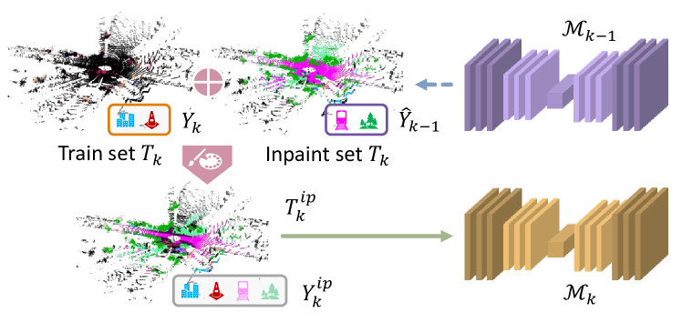
Figure 4: Background Self-Inpainting. Labels for old classes $C_{k-1}$ are predicted by previous model $\mathcal{M}_{k-1}$ and Inpainted onto background labels of current training set $T_{k}$.

4.2.1 Knowledge Distillation

Knowledge Distillation (KD) is the process of transferring knowledge from a model to another (typically smaller) [19, 20]. In our case, we apply knowledge distillation to recall past classes while learning new ones and to deal with the background shift phenomenon. Old labels are recovered from the previous step model $\mathcal{M}_{k-1}$. KD is modeled as an additional objective function $\mathcal{L}_{kd}$ tuned by a hyperparameter $\lambda$, obtaining as a final objective for model $\mathcal{M}_{k}$:

$$\mathcal{L}=\mathcal{L}_{ce}(y_{k},\hat{y}_{k})+\lambda\cdot\mathcal{L}_{kd}(\hat{y}_{k-1},\hat{y}_{k})$$ (2)

where $y_{k}$ are the ground truth labels of step $k$, $\hat{y}_{k}$ are the predictions of step $k$ and $\hat{y}_{k-1}$ are the prediction labels of step $k-1$. At step $k=0$ KD is not applied, as at that stage we lack any prior knowledge of past classes.

Output Level Distillation ($\mathcal{L}_{kd}$)

is typically modeled as an additional Cross-Entropy [17], where labels for past classes are obtained from previous model predictions:

$$\small\mathcal{L}_{kd}=-\frac{1}{|T_{k}|}\sum_{{\rm\bf X}_{n}\in T_{k}}\sum_{c\in C_{k-1}\cup C_{k}}\mathcal{M}_{k-1}({\rm\bf X}_{n})[c]\cdot\log(\mathcal{M}_{k}({\rm\bf X}_{n})[c])$$ (3)

where $\mathcal{M}_{k}({\rm\bf X}_{n})[c]$ and $\mathcal{M}_{k-1}({\rm\bf X}_{n})[c]$ are the prediction scores for class $c$, obtained with current and previous models, respectively. KD can be modeled either by masking predictions of each model $\mathcal{M}_{k}$ on classes $C_{k}$ or joining all the predictions of unknown classes [7]. An alternative formulation updates also the previous model to refine predictions [48]. For Coarse-to-Fine CL, the predictions for classes within the same coarse class are summed before applying the Cross-Entropy loss.

Cylinder3D
	Step 0	Step 1			Step 2
Method	mIoU0	mIoU0	mIoU1	mIoU0,1	mIoU0	mIoU1	mIoU2	mIoU0,1,2
Baseline†	—	—	—	—	—	—	—	54.1
Sequential	55.4	52.7	46.3	50.1	52.8	50.6	32.7	44.9
Sequential Masked	55.4	0.0	77.4	20.4	0.0	0.0	25.7	10.8
Disjoint	55.4	0.0	63.3	20.0	0.0	0.0	25.2	10.6
Output KD [29]	55.4	45.6	41.1	43.5	47.4	32.0	24.5	33.7
Self-Inpaint [32]	55.4	51.2	47.1	49.4	46.2	36.8	26.9	35.6

RandLA-Net
	Step 0	Step 1			Step 2
Method	mIoU0	mIoU0	mIoU1	mIoU0,1	mIoU0	mIoU1	mIoU2	mIoU0,1,2
Baseline†	—	—	—	—	—	—	—	47.2
Sequential	49.0	57.0	39.0	48.8	58.0	48.4	28.2	42.9
Sequential Masked	49.0	0.0	48.5	22.0	0.0	0.0	31.4	13.2
Disjoint	49.0	0.0	37.9	18.0	0.0	0.0	26.1	11.0
Output KD [29]	49.0	56.2	38.0	47.9	58.5	49.1	31.0	44.4
Self-Inpaint [32]	49.0	56.1	34.9	46.5	57.5	43.2	22.6	39.0

Table 2: Results of Cylinder3D and RandLA-Net (CIL). Bold denotes the best result, underline the second best. †: baselines retrained with our configuration.

method	car	bicycle	motorcycle	truck	other-vehicle	person	bicyclist	motorcyclist	road	parking	sidewalk	other-ground	building	fence	vegetation	trunk	terrain	pole	traffic-sign	mIoU $\uparrow$	Std Dev. $\sigma\downarrow$
Baseline†	90.7	1.6	14.6	53.9	37.1	30.5	54.2	0.0	90.9	35.4	75.1	2.2	84.0	46.3	84.9	47.1	69.7	51.7	27.6	47.2	30.1
Sequential	89.3	0.0	12.5	59.4	33.0	8.2	23.2	0.0	90.5	26.0	73.9	0.8	84.2	47.8	85.1	51.9	71.6	49.3	8.7	42.9	33.0
Output KD [29]	88.6	0.0	11.6	52.6	32.2	10.2	52.5	0.0	90.4	28.5	73.9	0.0	84.6	47.0	85.0	55.9	73.3	51.4	6.7	44.4	32.8
Output UKD [7]	88.0	0.0	7.3	27.2	17.8	0.9	16.9	0.0	90.3	29.8	74.3	2.5	83.3	47.4	84.8	50.8	72.8	44.0	1.3	38.9	34.3
Output XKD [48]	86.5	0.0	11.6	59.3	21.0	2.5	45.2	0.0	90.8	32.3	75.1	0.2	83.0	44.3	85.0	46.0	72.6	46.5	8.9	42.7	33.0
Feature KD (L2)	88.4	0.0	13.2	57.0	16.4	9.0	35.1	0.0	90.3	22.4	73.9	0.5	82.5	44.1	84.8	52.6	72.8	49.3	0.1	41.7	33.6
Feature KD (L1)	87.5	0.0	10.9	36.1	35.9	0.0	39.9	0.0	90.4	32.1	74.2	0.1	82.4	40.7	85.7	53.4	75.2	46.6	1.1	41.7	33.4
Both KD [36]	85.3	0.0	10.2	42.9	20.2	0.0	33.9	0.0	90.0	24.8	72.9	0.4	82.7	42.8	84.1	43.7	72.0	44.5	0.0	39.5	33.3
Self-Inpaint [32]	86.3	0.0	7.3	54.5	5.3	0.1	27.0	0.0	90.4	25.0	74.1	1.6	82.9	42.3	82.7	45.3	71.1	45.5	0.0	39.0	34.4

Table 3: Per-class mIoU results of RandLA-Net (CIL). Bold denotes the best result, underline the second best. †: baseline retrained with our configuration.

Feature Level Distillation ($\mathcal{L}^{*}_{kd}$)

is typically modeled as L_p (L₂ or L₁) norm between the features of current and previous models:

$$\mathcal{L}^{*}_{kd}=\frac{||\mathcal{E}_{k-1}({\rm\bf X}_{n})-\mathcal{E}_{k}({\rm\bf X}_{n})||_{p}}{|T_{k}|}$$ (4)

where $\mathcal{E}_{k}({\rm\bf X}_{n})[c]$ and $\mathcal{E}_{k-1}({\rm\bf X}_{n})[c]$ are the features of current and previous models, respectively. The choice of this design is motivated by the fact that this strategy provides learning of a feature map rather than a classification map and distance loss provides an alignment of such embeddings. KD at feature and output levels can be also combined to obtain joint effects from both.

4.2.2 Background Self-Inpainting

Background Self-Inpainting is a simple self-teaching mechanism that provides pseudo labeling of current background samples [32], reducing the background shift while bringing a regularization effect similar to knowledge distillation. At every step $k$ with training set $T_{k}$, we take the background points of each ground truth map $Y_{k}$ and we label it with the associated prediction from the previous model $\mathcal{M}_{k-1}$ (Fig. 4). More formally, we replace each original label map $Y_{k}$ available at step $k>0$ with its inpainted version $Y_{k}^{ip}$:

$${Y}_{k}^{ip}[i]=\begin{cases}{Y_{k}[i]}&\text{if}\quad{Y}[i]\in{C}_{k}\\ {\rho\cdot\hat{Y}_{k-1}[i]}&\text{otherwise}\end{cases}$$ (5)

where $(X_{k},Y_{k})\in T_{k}$. $[i]$ denotes $i$-th sample in $T_{k}$ and $\rho$ defines the inpaining rule. $\rho$ is designed as:

$$\rho=\begin{cases}1&\text{if}\quad\hat{\mathcal{Y}}^{*}_{k}[i]-\hat{\mathcal{Y}}^{**}_{k}[i]>\tau_{1}\quad\text{and}\quad\hat{\mathcal{Y}}^{*}_{k}[i]>\tau_{2}\\ 0&\quad\text{otherwise}.\end{cases}$$ (6)

$\hat{\mathcal{Y}}^{*}_{k}[i]$ and $\hat{\mathcal{Y}}^{**}_{k}[i]$ denote the sets of first and second maximum in the softmax predictions $\hat{\mathcal{Y}}_{k}$ at step $k$. Labels at step $k=0$ are not inpainted, as at that stage we lack any prior knowledge of past classes. When background inpainting is performed, each set $T^{ip}_{k}\subset X\times Y_{C_{0\rightarrow k}}$ ($k>0$) contains all samples of $T_{k}$ after being inpainted.

5 Experimental Results

For the experimental evaluation, we use RandLA-Net [21] (a widely used lightweight point based architecture) and compare results with Cylinder3D [53, 52] (state-of-the-art model based on voxels and point-wise prediction refinements). Note that the approach is generalizable to any other segmentation architecture for point clouds. We used SemanticKITTI [2, 16] as a reference dataset, with classes and data partitioned into learning steps according to CIL and C2F splits, described in Sec. 4.1. The model performance is measured by the mean Intersection over Union (mIoU) [31]. From now on, we use the notation mIoU_k to denote the mIoU computed on class set $C_{k}$.

We train both RandLA-Net and Cylinder3D using Adam optimizer with their standard learning rate policy, momentum, and weight decay. The initial learning rates are set respectively to $0.01$ and $0.001$ for the two models. The incremental training has been performed decreasing the learning rate according to a polynomial decay rule with power $0.95$. Note that at step $k$ the learning rate is initialized to the last learning rate of step $k-1$ to better preserve previous weights. We set batch size $3$ and train each learning step $k$ for a number of epochs $2\times|C_{k}|$, proportional to the number of new classes to be learned. We used PyTorch [39] for the implementation and train both models on NVIDIA GeForce RTX 3090Ti graphics processing unit with CUDA 11.6. The training of each learning step took around 5 hours with RandLA-Net and 30 hours with Cylinder3D. The code is available at: https://github.com/LTTM/CL-PCSS. In the following sections, we discuss the results obtained with CIL and C2F partitions. Baseline results are obtained by training the model from scratch on the whole dataset with all the classes, using the aforementioned configuration.

5.1 CIL

We performed our first set of experiments following CIL configuration. First, we developed standard fine-tuning methods, knowledge distillation, and self-inpainting to compare Cylinder3D with RandLA-Net. Results are reported in Tab. 2. In general, the obtained performances reflect the behavior of the corresponding image-based setups. As expected, the disjoint scenario performs the worst in all the learning steps, strongly suffering the background shift phenomenon. Sequential masked improves a little the results besides showing again the effect of catastrophic forgetting when accounting for new classes.

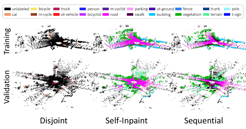
Figure 5: Some qualitative results on CIL with Cylinder3D.

Overall, Cylinder3D shows worse performance with respect to RandLA-Net within a CL framework, despite its better performance in the non-incremental scenario. Its results on the baseline show a strong performance decrease losing $9.8\%$ mIoU in the sequential setup (best case for fine-tuning). Besides, the size of the architecture and the processing of voxels make the training time 6 times longer. KD partially recovers knowledge from previous classes but keeps stability when learning new ones. Instead, Self-Inpainting is more performing and accounts better for new classes. Note that, mIoU₀ is efficiently recovered by both methods across the steps, while mIoU₁ is hardly restored. This is partially due to the fact that labels for step $k=0$ are robust classes with many points and a general method for catastrophic forgetting mitigation can be sufficient for recovering knowledge. Contrarily, step $k=1$ has a huge decrease in the number of labeled points that reflects the increasing difficulty in obtaining good recovery from previous training. Self-Inpainting hardly pseudo-labels old classes, not preserving the uncertainty of predictions, and penalizing the learning of new classes. The introduction of inpainting rules (Tab. 5) brings a slight improvement, avoiding strongly wrong predictions to be considered as true labels in the subsequent step. In this way, previous knowledge is hardly restored only in case of accurate predictions and blended into the current model in a stronger way with respect to KD. Finally, both methods perform worse with respect to the sequential setup. Qualitative results of the self-inpainting strategy are shown in Fig. 5.

	Step 0	Step 1			Step 2
Method	mIoU0	mIoU0	mIoU1	mIoU0,1	mIoU0	mIoU1	mIoU2	mIoU0,1,2
Baseline†	—	—	—	—	—	—	—	47.2
Overlapped	60.2	0.0	51.6	23.4	0.0	0.0	32.2	13.6
Disjoint	49.0	0.0	37.9	18.0	0.0	0.0	26.1	11.0
Output KD [29]	49.0	56.2	38.0	47.9	58.5	49.1	31.0	44.4
Output UKD [7]	49.0	56.1	35.3	46.6	59.1	45.4	19.8	38.9
Output XKD [48]	49.0	56.0	35.4	46.7	59.3	45.7	28.3	42.7
Feature KD (L2)	49.0	55.9	40.7	49.0	57.5	45.7	27.4	41.7
Feature KD (L1)	49.0	55.5	36.4	46.8	59.6	44.8	26.3	41.7
Both KD [36]	49.0	56.5	33.9	46.2	57.4	42.7	24.1	39.5

Table 4: RandLA-Net (CIL). Bold denotes the best result, underline the second best. †: baseline retrained with our configuration.

		Step 0	Step 1			Step 2
$\boldsymbol{\tau_{1}}$	$\boldsymbol{\tau_{2}}$	mIoU0	mIoU0	mIoU1	mIoU0,1	mIoU0	mIoU1	mIoU2	mIoU0,1,2
0	0	55.4	50.7	39.6	45.8	47.7	42.8	19.4	34.5
0	0.7	55.4	48.4	37.9	43.6	44.0	38.7	25.0	34.6
0.2	0	55.4	55.8	40.5	48.9	45.2	35.9	28.0	35.5
0.2	0.7	55.4	51.2	47.1	49.4	46.2	36.8	26.9	35.6

Table 5: Ablation study on Self-Inpainting with Cylinder3D. $\tau_{1},\tau_{2}$ are the parameters for inpainting. Bold denotes the best result.

	Step 0	Step 1		Step 2
Method	mIoU0	mIoU0	mIoU1	mIoU0	mIoU1	mIoU2
Baseline†	—	—	—	—	—	47.2
Fine-Tuning	86.7	74.6	74.6	51.0	51.0	47.1
Output KD	86.7	52.9	52.9	48.8	48.8	45.1
Feature KD (L1)	86.7	57.2	57.2	47.1	47.1	42.8

Table 6: RandLA-Net on SemanticKITTI (C2F). Bold denotes the best result. †: baseline retrained with our configuration.

method	car	bicycle	motorcycle	truck	other-vehicle	person	bicyclist	motorcyclist	road	parking	sidewalk	other-ground	building	fence	vegetation	trunk	terrain	pole	traffic-sign	mIoU $\uparrow$	Std Dev. $\sigma\downarrow$
Baseline†	90.7	1.6	14.6	53.9	37.1	30.5	54.2	0.0	90.9	35.4	75.1	2.2	84.0	46.3	84.9	47.1	69.7	51.7	27.6	47.2	30.1
Fine-Tuning	89.7	6.2	17.4	47.0	24.8	28.3	65.5	0.0	88.8	30.7	73.0	0.6	83.6	45.8	87.2	55.4	75.1	50.8	24.4	47.1	30.7
Output KD	90.3	0.2	16.6	53.2	30.0	14.8	42.1	0.0	90.7	26.9	74.1	0.1	84.5	43.9	86.5	56.8	73.9	52.0	21.1	45.1	31.9
Feature KD (L1)	89.2	0.0	12.5	65.7	29.6	3.6	41.4	0.0	91.2	37.9	74.3	0.8	84.8	45.4	86.2	50.1	72.9	48.7	18.2	44.9	32.7

Table 7: Per-class mIoU results on C2F with RandLA-Net. Bold denotes the best result. †: baseline retrained with our configuration.

step	car	bicycle	motorcycle	truck	other-vehicle	person	bicyclist	motorcyclist	road	parking	sidewalk	other-ground	vegetation	terrain	building	fence	trunk	pole	traffic-sign	mIoU $\uparrow$ [31]	Std Dev. $\sigma\downarrow$	PA $\uparrow$ [22]	PP $\uparrow$ [27]
0	85.1								95.6						79.5					86.7	8.2	93.0	92.6
1	89.1					43.4			92.2				89.8		81.7		51.3			74.6	21.5	80.4	89.6
2	89.7	6.2	17.4	47.0	24.8	28.3	65.5	0.0	88.8	30.7	73.0	0.6	87.2	75.1	83.6	45.8	55.4	50.8	24.4	47.1	30.7	56.2	67.7

Table 8: Per-class Coarse-to-Fine results, standard fine-tuning. Different colors are associated with different Coarse partitions.

On the other hand, RandLA-Net shows great suitability for continual learning settings, with a decrease of only $4.7\%$ mIoU in the sequential setup, with respect to the baseline. Surprisingly, recovering knowledge via distillation obtains $44.4\%$ mIoU, improving the sequential setup of $1.5\%$ mIoU with a gap from the baseline of only $2.8\%$ mIoU. This is again a consequence of the label frequency of each split: early steps have a large number of labeled samples, while later steps contain only a few labeled samples. The network is subject to this imbalance when it is trained only with $\mathcal{L}_{ce}$, both in sequential Fine-Tuning and Self-Inpainting.

For this extent, we led extensive experiments with RandLA-Net on Knowledge Distillation, considering both the case of Distilling output predictions and intermediate features. Tab. 4 reports the overall mIoU results across learning steps, while Tab. 3 reports per-class results in the final learning step. Both distillation methods consistently improve the overall results. The overall best solution is represented by the standard output level distillation, but also KD at the feature level performs quite well. However, in general, per-class results show that the incremental setup emphasizes the gap in performance between frequent and infrequent classes. For example, class car obtains always good results around $90\%$ mIoU, while class bicycle (belonging to the same partition) obtains $1.6\%$ mIoU on the baseline but is never classified correctly in the incremental setup. Similarly, traffic-sign obtains $27.6\%$ mIoU in the baseline but its performance decrease drastically when incremental learning is applied; in Self-inpainting it is never classified correctly. Indeed, the lowest standard deviation is achieved by the baseline model.

Finally, worth to be mentioned is the result of the Overlapped setup (reported in Tab. 4) in comparison with the Disjoint one: training on the whole dataset brings as expected an improvement ($2.6\%$ on the final mIoU) but still suffers for catastrophic forgetting.

5.2 Coarse-to-Fine

Results on the Coarse-to-Fine partition are reported in Tab. 7. Fine-tuning on coarse classes obtains results comparable with the standard baseline training ($47.1\%$ vs $47.2\%$ mIoU), despite a higher standard deviation among classes. Note that this tuning is performed on the split sequences of Tab. 1, while general Coarse-to-Fine approaches rely on the Overlapped approach. Contrarily to CIL, a direct application of Knowledge Distillation leads here to poor performance, both when applied at the output level and intermediate feature space, losing $2.0\%$ and $2.2\%$ mIoU respectively. Hence, this setting requires the application of more sophisticated loss functions in order to obtain a substantial improvement. Tab. 8 reports the results of the C2F fine-tuning in terms of mIoU, Point Accuracy (PA) [22] and Point Precision (PP) [27]. Results in the first step achieve higher accuracy with a low standard deviation, which increases with learning steps (classes are fairly distributed up to step $k=1$). This result suggests that additional intermediate steps could be beneficial to improve the final performance, which in general requires further refinement.

6 Conclusion

The paper tackled the problem of class incremental continual learning for LiDAR semantic segmentation. We formally partitioned SemanticKITTI into semantically-consistent groups, and we evaluated partitions on CL strategies addressing different techniques to prevent catastrophic forgetting. A comparison of RandLA-Net and Cylinder3D performance shows that the former (point based and lightweight) fits better into the class-incremental setup. Experiments on our proposed subdivision of SemanticKITTI prove the efficiency of CL strategies in alleviating catastrophic forgetting, even on sparse data. The overall problem still requires improvements as the performance is lower than the ones achieved after standard single-step training. Future work will expand the experimental framework by introducing class balancing constraints among previous and current experiences, and geometric constraints, designed ad hoc for LiDAR point clouds.

References

- [1] Iro Armeni, Ozan Sener, Amir R Zamir, Helen Jiang, Ioannis Brilakis, Martin Fischer, and Silvio Savarese. 3D semantic parsing of large-scale indoor spaces. In CVPR, pages 1534–1543, 2016.
- [2] J. Behley, M. Garbade, A. Milioto, J. Quenzel, S. Behnke, C. Stachniss, and J. Gall. SemanticKITTI: A Dataset for Semantic Scene Understanding of LiDAR Sequences. In Proc. of the IEEE/CVF International Conf. on Computer Vision (ICCV), 2019.
- [3] Elena Camuffo, Daniele Mari, and Simone Milani. Recent advancements in learning algorithms for point clouds: An updated overview. Sensors, 22(4):1357, 2022.
- [4] Elena Camuffo, Umberto Michieli, and Simone Milani. Learning from mistakes: Self-regularizing hierarchical semantic representations in point cloud segmentation. arXiv preprint arXiv:2301.11145, 2023.
- [5] Jun Cen, Peng Yun, Shiwei Zhang, Junhao Cai, Di Luan, Michael Yu Wang, Ming Liu, and Mingqian Tang. Open-world semantic segmentation for lidar point clouds. arXiv preprint arXiv:2207.01452, 2022.
- [6] Fabio Cermelli, Dario Fontanel, Antonio Tavera, Marco Ciccone, and Barbara Caputo. Incremental learning in semantic segmentation from image labels. In CVPR, June 2022.
- [7] Fabio Cermelli, Massimiliano Mancini, Samuel Rota Bulo, Elisa Ricci, and Barbara Caputo. Modeling the background for incremental learning in semantic segmentation. In Proceedings of the IEEE Conference on Computer Vision and Pattern Recognition (CVPR), pages 9233–9242, 2020.
- [8] Townim Chowdhury, Ali Cheraghian, Sameera Ramasinghe, Sahar Ahmadi, Morteza Saberi, and Shafin Rahman. Few-shot class-incremental learning for 3d point cloud objects. ECCV, pages 204–220, 10 2022.
- [9] Marius Cordts, Mohamed Omran, Sebastian Ramos, Timo Rehfeld, Markus Enzweiler, Rodrigo Benenson, Uwe Franke, Stefan Roth, and Bernt Schiele. The cityscapes dataset for semantic urban scene understanding. In Proceedings of the IEEE Conference on Computer Vision and Pattern Recognition (CVPR), June 2016.
- [10] Tiago Cortinhal, George Tzelepis, and Eren Erdal Aksoy. Salsanext: Fast, uncertainty-aware semantic segmentation of lidar point clouds for autonomous driving, 2020.
- [11] Matthias De Lange, Rahaf Aljundi, Marc Masana, Sarah Parisot, Xu Jia, Aleš Leonardis, Gregory Slabaugh, and Tinne Tuytelaars. A continual learning survey: Defying forgetting in classification tasks. IEEE Transactions on Pattern Analysis and Machine Intelligence, 44(7):3366–3385, 2022.
- [12] Jiahua Dong, Yang Cong, Gan Sun, Bingtao Ma, and Lichen Wang. I3dol: Incremental 3d object learning without catastrophic forgetting. In AAAI Conference on Artificial Intelligence, 2020.
- [13] Arthur Douillard, Yifu Chen, Arnaud Dapogny, and Matthieu Cord. Plop: Learning without forgetting for continual semantic segmentation. In CVPR, 2021.
- [14] Hehe Fan, Xin Yu, Yuhang Ding, Yi Yang, and Mohan Kankanhalli. PSTNet: Point spatio-temporal convolution on point cloud sequences. ICLR, 2021.
- [15] Biao Gao, Yancheng Pan, Chengkun Li, Sibo Geng, and Huijing Zhao. Are we hungry for 3d lidar data for semantic segmentation? a survey of datasets and methods. IEEE Transactions on Intelligent Transportation Systems, 2021.
- [16] A. Geiger, P. Lenz, and R. Urtasun. Are we ready for Autonomous Driving? The KITTI Vision Benchmark Suite. In Proceedings of the IEEE Conference on Computer Vision and Pattern Recognition (CVPR), pages 3354–3361, 2012.
- [17] I. J. Good. Rational decisions. Journal of the Royal Statistical Society. Series B (Methodological), 14(1):107–114, 1952.
- [18] Meng-Hao Guo, Jun-Xiong Cai, Zheng-Ning Liu, Tai-Jiang Mu, Ralph R. Martin, and Shi-Min Hu. Pct: Point cloud transformer. Computational Visual Media, 7(2):187–199, Apr 2021.
- [19] Geoffrey Hinton, Oriol Vinyals, and Jeff Dean. Distilling the knowledge in a neural network. WACV, 2015.
- [20] Yuenan Hou, Xinge Zhu, Yuexin Ma, Chen Change Loy, and Yikang Li. Point-to-voxel knowledge distillation for lidar semantic segmentation. In IEEE Conference on Computer Vision and Pattern Recognition, pages 8479–8488, 2022.
- [21] Qingyong Hu, Bo Yang, Linhai Xie, Stefano Rosa, Yulan Guo, Zhihua Wang, Niki Trigoni, and Andrew Markham. Randla-net: Efficient semantic segmentation of large-scale point clouds. Proceedings of the IEEE Conference on Computer Vision and Pattern Recognition, 2020.
- [22] Matthew Johnson-Roberson, Charlie Barto, Rounak Mehta, Sharath Nittur Sridhar, Karl Rosaen, and Ram Vasudevan. Driving in the matrix: Can virtual worlds replace human-generated annotations for real world tasks? ICRA, pages 746–753, 2016.
- [23] KJ Joseph, Salman Khan, Fahad Shahbaz Khan, and Vineeth N Balasubramanian. Towards open world object detection. In Proceedings of the IEEE Conference on Computer Vision and Pattern Recognition (CVPR), pages 5830–5840, 2021.
- [24] James Kirkpatrick, Razvan Pascanu, Neil Rabinowitz, Joel Veness, Guillaume Desjardins, Andrei A. Rusu, Kieran Milan, John Quan, Tiago Ramalho, Agnieszka Grabska-Barwinska, Demis Hassabis, Claudia Clopath, Dharshan Kumaran, and Raia Hadsell. Overcoming catastrophic forgetting in neural networks. Proceedings of the National Academy of Sciences, 114(13):3521–3526, 2017.
- [25] Marvin Klingner, Andreas Bär, Philipp Donn, and Tim Fingscheidt. Class-incremental learning for semantic segmentation re-using neither old data nor old labels. In 2020 IEEE 23rd International Conference on Intelligent Transportation Systems (ITSC), pages 1–8. IEEE, 2020.
- [26] Joshua Knights, Peyman Moghadam, Milad Ramezani, Sridha Sridharan, and Clinton Fookes. Incloud: Incremental learning for point cloud place recognition. In 2022 IEEE/RSJ International Conference on Intelligent Robots and Systems (IROS), pages 8559–8566. IEEE, 2022.
- [27] Alex Lang, Sourabh Vora, Holger Caesar, Lubing Zhou, Jiong Yang, and Oscar Beijbom. Pointpillars: Fast encoders for object detection from point clouds. Proceedings of the IEEE Conference on Computer Vision and Pattern Recognition (CVPR), pages 12689–12697, 06 2019.
- [28] Junnan Li, Pan Zhou, Caiming Xiong, and Steven CH Hoi. Prototypical contrastive learning of unsupervised representations. In ICLR, 2021.
- [29] Zhizhong Li and Derek Hoiem. Learning without forgetting. IEEE Transactions on Pattern Analysis and Machine Intelligence, 40:2935–2947, 2016.
- [30] Yaping Lin, George Vosselman, Yanpeng Cao, and Michael Ying Yang. Active and incremental learning for semantic als point cloud segmentation. ISPRS Journal of Photogrammetry and Remote Sensing, 169:73–92, 2020.
- [31] Jonathan Long, Evan Shelhamer, and Trevor Darrell. Fully convolutional networks for semantic segmentation. Proceedings of the IEEE Conference on Computer Vision and Pattern Recognition (CVPR), pages 3431–3440, 2015.
- [32] Andrea Maracani, Umberto Michieli, Marco Toldo, and Pietro Zanuttigh. Recall: Replay-based continual learning in semantic segmentation. In Proceedings of the IEEE/CVF International Conference on Computer Vision, pages 7026–7035, 2021.
- [33] Daniel Maturana and Sebastian Scherer. Voxnet: A 3d convolutional neural network for real-time object recognition. In 2015 IEEE/RSJ International Conference on Intelligent Robots and Systems (IROS), pages 922–928, 2015.
- [34] Mazen Mel, Umberto Michieli, and Pietro Zanuttigh. Incremental and multi-task learning strategies for coarse-to-fine semantic segmentation. Technologies, 8(1):1, 2020.
- [35] Umberto Michieli, Marco Toldo, and Pietro Zanuttigh. Chapter 8 - domain adaptation and continual learning in semantic segmentation. In E.R. Davies and Matthew A. Turk, editors, Advanced Methods and Deep Learning in Computer Vision, Computer Vision and Pattern Recognition, pages 275–303. Academic Press, 2022.
- [36] Umberto Michieli and Pietro Zanuttigh. Incremental learning techniques for semantic segmentation. In International Conference on Computer Vision (ICCV), Workshop on Transferring and Adapting Source Knowledge in Computer Vision (TASK-CV), 2019.
- [37] Umberto Michieli and Pietro Zanuttigh. Continual semantic segmentation via repulsion-attraction of sparse and disentangled latent representations. In Proceedings of the IEEE Conference on Computer Vision and Pattern Recognition (CVPR), pages 1114–1124, 2021.
- [38] Andres Milioto, Ignacio Vizzo, Jens Behley, and Cyrill Stachniss. Rangenet++: Fast and accurate lidar semantic segmentation. In IROS, pages 4213–4220. IEEE, 2019.
- [39] Adam Paszke, Sam Gross, Francisco Massa, Adam Lerer, James Bradbury, Gregory Chanan, Trevor Killeen, Zeming Lin, Natalia Gimelshein, Luca Antiga, Alban Desmaison, Andreas Kopf, Edward Yang, Zachary DeVito, Martin Raison, Alykhan Tejani, Sasank Chilamkurthy, Benoit Steiner, Lu Fang, Junjie Bai, and Soumith Chintala. Pytorch: An imperative style, high-performance deep learning library. In Advances in Neural Information Processing Systems 32, pages 8024–8035. Curran Associates, Inc., 2019.
- [40] Can Peng, Kun Zhao, and Brian C. Lovell. Faster ilod: Incremental learning for object detectors based on faster rcnn. Pattern Recognition Letters, 140:109–115, 2020.
- [41] Charles R Qi, Hao Su, Kaichun Mo, and Leonidas J Guibas. Pointnet: Deep learning on point sets for 3d classification and segmentation. Proceedings of the IEEE Conference on Computer Vision and Pattern Recognition (CVPR), 2016.
- [42] Charles R Qi, Li Yi, Hao Su, and Leonidas J Guibas. Pointnet++: Deep hierarchical feature learning on point sets in a metric space. NeurIPS, 2017.
- [43] Sylvestre-Alvise Rebuffi, Alexander Kolesnikov, Georg Sperl, and Christoph Lampert. icarl: Incremental classifier and representation learning. pages 5533–5542, 07 2017.
- [44] Donald Shenaj, Francesco Barbato, Umberto Michieli, and Pietro Zanuttigh. Continual coarse-to-fine domain adaptation in semantic segmentation. Image and Vision Computing, 121:104426, 2022.
- [45] Konstantin Shmelkov, Cordelia Schmid, and Karteek Alahari. Incremental learning of object detectors without catastrophic forgetting. In 2017 IEEE International Conference on Computer Vision (ICCV), pages 3420–3429, 2017.
- [46] Otilia Stretcu, Emmanouil Antonios Platanios, Tom Mitchell, and Barnabás Póczos. Coarse-to-fine curriculum learning for classification. In ICLRW, 2020.
- [47] Lyne P. Tchapmi, Christopher Bongsoo Choy, Iro Armeni, JunYoung Gwak, and Silvio Savarese. Segcloud: Semantic segmentation of 3d point clouds. 2017 International Conference on 3D Vision (3DV), pages 537–547, 2017.
- [48] Marco Toldo, Umberto Michieli, and Pietro Zanuttigh. Learning with style: Continual semantic segmentation across tasks and domains. 2022.
- [49] Xiang Xiang, Yuwen Tan, Qian Wan, Jing Ma, Alan Yuille, and Gregory D Hager. Coarse-to-fine incremental few-shot learning. In Computer Vision–ECCV 2022: 17th European Conference, Tel Aviv, Israel, October 23–27, 2022, Proceedings, Part XXXI, pages 205–222. Springer, 2022.
- [50] Boyu Yang, Fang Wan, Chang Liu, Bohao Li, Xiangyang Ji, and Qixiang Ye. Part-based semantic transform for few-shot semantic segmentation. IEEE Transactions on Neural Networks and Learning Systems, 2021.
- [51] Yang Zhang, Zixiang Zhou, Philip David, Xiangyu Yue, Zerong Xi, Boqing Gong, and Hassan Foroosh. Polarnet: An improved grid representation for online lidar point clouds semantic segmentation. In Proceedings of the IEEE Conference on Computer Vision and Pattern Recognition (CVPR), pages 9601–9610, 2020.
- [52] Xinge Zhu, Hui Zhou, Tai Wang, Fangzhou Hong, Wei Li, Yuexin Ma, Hongsheng Li, Ruigang Yang, and Dahua Lin. Cylindrical and asymmetrical 3d Convolution Networks for lidar-based perception. IEEE Transactions on Pattern Analysis and Machine Intelligence, 2021.
- [53] Xinge Zhu, Hui Zhou, Tai Wang, Fangzhou Hong, Yuexin Ma, Wei Li, Hongsheng Li, and Dahua Lin. Cylindrical and asymmetrical 3d convolution networks for lidar segmentation. In IEEE Conference on Computer Vision and Pattern Recognition, pages 9939–9948, 2021.