The $n$-vehicle exploration problem is NP-complete

Abstract

The $n$-vehicle exploration problem (NVEP) is a combinatorial optimization problem, which tries to find an optimal permutation of a fleet to maximize the length traveled by the last vehicle. NVEP has a fractional form of objective function, and its computational complexity of general case remains open. We show that Hamiltonian path $\leq_{P}$ NVEP, and consequently prove that NVEP is NP-complete.

1 Introduction

The $n$-vehicle exploration problem (NVEP) is motivated by a problem in a contest puzzle in China [7]: there are $n$ vehicles $V_{1},\cdots,V_{n}$ with fuel capacities $a_{i}$ and fuel consumption rates $b_{i}$ for $(1\leq i\leq n)$. It is assumed that these $n$ vehicles start toward the same direction from the same point at the same time. During the trip, they can not get fuel from outside, but at any point any vehicle can stop and transfer its remaining fuel to other vehicles. The goal is to determine a drop out permutation $\pi=\{\pi(1),\cdots,\pi(n)\}$ and its related sequence $V_{\pi}=\{V_{\pi(1)},\cdots,V_{\pi(n)}\}$ that maximize the traveled length by the last vehicle. Then given an arbitrary drop out order $\pi$, the traveled length of sequence $V_{\pi}$ is

(1) $$\sum\limits_{j=1}^{n}(a_{\pi(j)}/\sum\limits_{k=j}^{n}b_{\pi(k)}).$$

A special characteristic of model (1) is that it has a fractional form of objective function with different permutation of vehicles. Such kind of model is the same with model of the airplane refueling problem[6], which is considered as an equivalent problem of NVEP. The cases where all vehicles have identical fuel capacities and where all vehicles have identical fuel consumption rates can be solved by sorting, but the computational complexity of the general case is still open [6]. Most of research on NVEP and its related problems focused on algorithm design and resorted to heuristic algorithm, approximation algorithm, or branch and bound technique. Gamzu and Segev [1] proposed a polynomial-time approximation scheme for airplane refueling problem with exhaustive computational complexity. Li et. [4] posed a fast exact algorithm for airplane refueling problem which executes effectively for some large scale instances. However, to our knowledge, there is no literature until now has proved the NP-completeness of NVEP.

In this paper we concentrate our efforts on proving the NP-completeness of NVEP. It is hard for us to reduce a known NP-complete problem [2] to NVEP. We finally choose Hamiltonian path to reduce to NVEP when we regard NVEP as a directed graph. Here a Hamiltonian path in a directed graph is a directed path which passes through each vertex exactly once, but need not to return to its starting point [5][3]. We show that each Hamiltonian path of a directed graph is equivalent to a running order of NVEP. Thus we prove the NP-completeness of NVEP, and the equivalent problems of NVEP are probably computationally intractable.

2 Preliminaries

Suppose the trail sequence is determined, and let $V_{\pi}$ denote the running sequence. In a sequence$\{V_{\pi(1)},\cdots,V_{\pi(n)}\}$, $V_{\pi(i)}$ always refuels to $V_{\pi(j)}$ for $i<j$. Let $D_{\pi}$ denote the longest running distance associated with sequence $V_{\pi}$, then the optimal solution for the running order $\pi$ is:

(2) $$D_{\pi}=\sum\limits_{j=1}^{n}{d_{\pi(j)}}=\sum\limits_{j=1}^{n}{\Big{(}a_{\pi(j)}\bigg{/}\sum\limits_{k=j}^{n}{b_{\pi(k)}}\Big{)}}$$

Each $D_{\pi}$ corresponds to a permutation of $n$ vehicles, so there supposed to be $n!$ alternatives of $D_{\pi}$, which requires a search of all the alternatives before we could be sure of finding the optimal solution.

Given a new problem $X$, here is the basic strategy proving it is NP-complete [3].

• Prove that $X\in NP$.

• Choose a problem $Y$ that is known to be NP-complete.

• Consider an arbitrary instance $S_{Y}$ of problem $Y$, and show how to construct, in polynomial time, an instance $S_{X}$ of problem $X$ that satisfies the following properties:

  • If $S_{Y}$ is a ”yes” instance of $Y$, then $S_{X}$ is a ”yes” instance of $X$.

  • If $S_{X}$ is a ”yes” instance of $X$, then $S_{Y}$ is a ”yes” instance of $Y$.

3 Main result

We present the decision version of the Hamiltonian path [3]:

Instance: Given a directed graph $G=(V,E)$.

Question: Is there a Hamiltonian path $P$ in $G$ that contains each vertex exactly once? (The path is allowed to start at any node and end at any node.)

Let us regard each node $v_{i}$ in $G$ as vehicle $V_{i}$, and each edge $(v_{i},v_{j})$ as a pair of vehicles $V_{i}\Rightarrow V_{j}$ (denotes that $V_{i}$ refuels to $V_{j}$) in a running order. For a directed graph $G=(V,E)$ with $4$ nodes and its related $4$-vehicle exploration problem are shown in Fig. 1

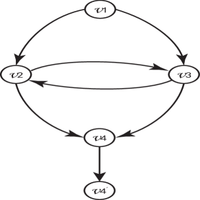
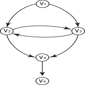
Figure 1: A subgraph of Hamiltonian path from $v_{1}$ to $v_{4}$ Versus. a $4$-vehicle sequence from $V_{1}$ to $V_{4}$. Here $v_{4}^{{}^{\prime}}$ is not a node but an exit point from $v_{4}$, and $V_{4}^{{}^{\prime}}$ is not a vehicle but a destination point that $V_{4}$ can reach.

There are $2$ Hamiltonian paths in Fig. 1$(a)$ as $v_{1}\rightarrow v_{2}\rightarrow v_{3}\rightarrow v_{4}\rightarrow v_{4}^{{}^{\prime}}$ and $v_{1}\rightarrow v_{3}\rightarrow v_{2}\rightarrow v_{4}\rightarrow v_{4}^{{}^{\prime}}$, Which are correspond to $2$ running orders as $V_{1}\Rightarrow V_{2}\Rightarrow V_{3}\Rightarrow V_{4}\Rightarrow V_{4}^{{}^{\prime}}$ and $V_{1}\Rightarrow V_{3}\Rightarrow V_{2}\Rightarrow V_{4}\Rightarrow V_{4}^{{}^{\prime}}$ in Fig. 1$(b)$. When we allow the Hamiltonian path start at any node and end at any node, then there should be $4$ start nodes and correspond to $3$ end nodes. So there are $4\times 3=12$ similar options of subgraphs as in Fig. 1$(a)$, and consequently totally $24$ Hamiltonian paths. For its related $4$-vehicle exploration instance, there are totally $24$ possible running orders.

For a directed graph $G=(V,E)$ with $5$ nodes and its related $5$-vehicle exploration problem are shown in Fig. 2.

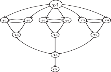
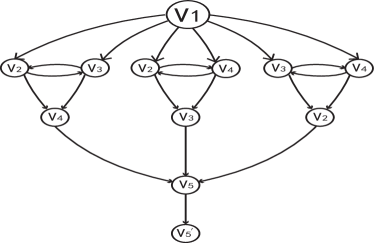
Figure 2: A subgraph of Hamiltonian path from $v_{1}$ to $v_{5}$ Versus. a $5$-vehicle sequence from $V_{1}$ to $V_{5}$. Here $v_{5}^{{}^{\prime}}$ is not a node but an exit point from $v_{5}$, and $V_{5}^{{}^{\prime}}$ is not a vehicle but a destination point that $V_{5}$ can reach.

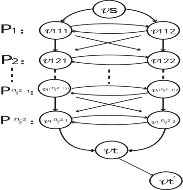
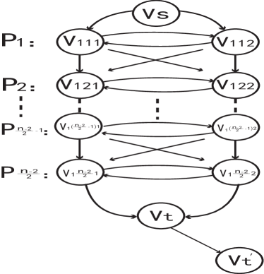
Figure 3: A subgraph of Hamiltonian path from $v_{s}$ to $v_{t}$ Versus. an $n$-vehicle sequence from $V_{s}$ to $V_{t}$. For each node $v_{ijk}$ and each vehicle $V_{ijk}$, it has $i=1,\cdots,(n-2)!/2^{\frac{n-2}{2}}$, $j=1,\cdots,\frac{n-2}{2}$, and $k=1,2$. Here $v_{t}^{{}^{\prime}}$ is not a node but an exit point from $v_{t}$, and $V_{t}^{{}^{\prime}}$ is not a vehicle but a destination point that $V_{t}$ can reach.

There are $6$ Hamiltonian paths in Fig. 2$(a)$ and $6$ sequences in Fig. 2$(b)$. When we allow the Hamiltonian path start at any node and end at any node, then there might be $5$ start nodes and correspond to $4$ end nodes. So there are $5\times 4=20$ similar options of subgraphs as in Fig. 2$(a)$, and consequently totally $120$ Hamiltonian paths. For its related $5$-vehicle exploration instance, there are totally $120$ possible running orders.

Let us consider a graph with $n$ nodes (assuming $n$ is an even number) and its related NVEP instances.

We show the restriction process from Fig. 3$(a)$ to Fig. 3$(b)$ as follows. We construct $\frac{n-2}{2}$ layers $P_{1},\cdots,P_{\frac{n-2}{2}}$, where $P_{j}$ consists of $2$ nodes $v_{ij1}$, $v_{ij2}$ (or $2$ vehicles $V_{ij1}$, $V_{ij2}$). There are edges from $v_{ij1}$ to $v_{ij2}$, and in the other direction from $v_{ij2}$ to $v_{ij1}$. Thus $P_{j}$ can be traversed ”left to right”, from $v_{ij1}$ to $v_{ij2}$, or ”right to left”, from $v_{ij2}$ to $v_{ij1}$. For each $j=1,2,\ldots,\frac{n-2}{2}-1$, we define edges from $v_{ij1}$ to $v_{i(j+1)1}$ and to $v_{i(j+1)2}$. We also define edges from $v_{ij2}$ to $v_{i(j+1)1}$ and to $v_{i(j+1)2}$. A Hamiltonian path starts at $v_{s}$ and ends at $v_{t}$, and we define edges from $v_{s}$ to $v_{i11}$ and $v_{i12}$; from $v_{i\frac{n-2}{2}1}$ and $v_{i\frac{n-2}{2}2}$ to $v_{t}$. A Hamiltonian path must start from $v_{s}$, after entering $v_{s}$, the ordering can then traverse $P_{1}$ either left to right or right to left, regardless of what it does here, it can then traverse $P_{2}$ either left to right or right to left; and so forth, until it finishes traversing $P_{\frac{n-2}{2}}$ and enters $v_{t}$. Therefore, there are exactly $2^{\frac{n-2}{2}}$ different Hamiltonian paths. A directed graph $G=(V,E)$ contains $n!/2^{\frac{n-2}{2}}$ subgraphs as shown in Fig. 3$(a)$. Thus there are $n!$ Hamiltonian paths for $G$.

Theorem 3.1.

NVEP is NP-complete.

Proof 3.2.

It is easy to see that NVEP is in $\mathcal{NP}$: The certificate could be a permutation of the vehicles, and a certifier checks that the running order contains each vehicle exactly once and the length of the corresponding trip is equal to $n$.

We now show that Hamiltonian Path $\leq_{P}$ NVEP, and we aim to show that any arbitrary Hamiltonian path can be reduced, in polynomial time, to a feasible permutation of vehicles of length $n$. Given a directed graph $G=(V,E)$ as shown in Fig. 3$(a)$, we define the following instance of NVEP. We have a vehicle $V_{i}$ for each node $v_{i}$ in graph $G$. We define $d(V_{i},V_{j})$ to be $1$ if there is an edge $(v_{i},v_{j})$ in $G$, and we define it to be $0$ otherwise. We add a virtual node $v_{t}^{{}^{\prime}}$ and a direct edge $v_{t}\rightarrow v_{t}^{{}^{\prime}}$. Similarly we define a virtual vehicle $V_{t}^{{}^{\prime}}$ as a destination vehicle, and we define $d(V_{t},V_{t}^{{}^{\prime}})=1$. Now we claim that $G$ has a Hamiltonian path if and only if there is a sequence of length that is equal to $n$ in our NVEP instance. For an arbitrary Hamiltonian path $P=\{v_{i_{1}},v_{i_{2}},\cdots,v_{i_{n}}\}$, there is a corresponding permutation of nodes, which leads to a permutation of vehicles belongs to an NVEP instance according to the following Algorithm 1.

Algorithm 1 Algorithm to get an NVEP instance in polynomial time

  Given an arbitrary Hamiltonian path $P=\{v_{i_{1}},v_{i_{2}},\cdots,v_{i_{n}}\}$

  A permutation of vehicles $\pi=\{V_{i_{1}},V_{i_{2}},\cdots,V_{i_{n}}\}$ corresponding to $P$

  Set $a_{i_{1}}=n,a_{i_{2}}=n-1,\cdots,a_{i_{n}}=1$

  Set $b_{i_{1}}=b_{i_{2}}=\cdots=b_{i_{n}}=1$

  According to equation (2), $D_{\pi}=\frac{a_{i_{1}}}{b_{i_{1}}+\cdots+b_{i_{n}}}+\cdots+\frac{a_{i_{n}}}{b_{i_{n}}}$

  return  $D_{\pi}=n$

According to Algorithm 1, an arbitrary Hamiltonian path $P$ is ”spread” to NVEP by constructing a permutation $\pi$, which is a feasible solution of NVEP that its corresponding running distance $D_{\pi}$ is no less than (actually equals to) $n$. A following result is that each term of $d_{\pi}$ must equal to $1$. Now we claim that $G$ has a Hamiltonian path if and only if there is a sequence of length that is equal to $n$ in our NVEP instance. The ordering $\pi$ determined by Algorithm 1 leads to $D_{\pi}$ equals to $n$.

Conversely, suppose there is a sequence of length equal to $n$ for the above NVEP instance. The length is a sum of $n$ terms, each of which must be equal to $1$. Hence each pair of nodes in $G$ that correspond to the consecutive vehicles in the sequence must be connected by an edge, and the ordering of these corresponding nodes must form a Hamiltonian path.

4 Conclusion

Proving the NP-completeness of the NVEP and its equivalent combinatorial optimization problems has shown particular difficulties before. The main difficulty is obvious which is caused by the fractional form of objective function. We reduce Hamiltonian path to NVEP and consequently prove that NVEP is NP-complete.

References

- [1] G. Iftah and S. Danny, A polynomial-time approximateion shceme for the airplane refueling problem, J. Sched., 22 (2019), pp. 429–444.
- [2] R. M. Karp, Reducibility among combinatorial problems, Complexity of Computations, R.E. Miller and J.W.Thatcher (eds.), New York: Plenum Press (1972), pp. 85–104.
- [3] J. Kleinberg and É. Tardos, Algorithm design, Pearson Education Asia Limited and Tsinghua University Press, Cornell University, 2006.
- [4] J. Li, X. Hu, J. Luo, and J. Cui, A fast exact algorithm for airplane refueling problem, Combinatorial Optimization and Applications, Proceedings, LNCS 11949, Springer Internaticonal Publishing (2019), pp. 316–327.
- [5] D. S. J. Michael R. Garey, Computers and intractability: a guide to the theory of NP-Completeness, W. H. Freeman and Company, New York, 1979.
- [6] G. J. Woeginger, The airplane refueling problem. Scheduling: Dagstuhl Seminar Proceedings 10071, Apr. 2010.
- [7] R. Yang, A travelling problem and its extended research, Bulletin of Maths, 9 (1999), pp. 44–45.