Quantum dynamics as a pseudo-density matrix

Abstract

While in relativity theory space evolves over time into a single entity known as spacetime, quantum theory lacks a standard notion of how to encapsulate the dynamical evolution of a quantum state into a single "state over time". Recently it was emphasized in the work of Fitzsimons, Jones and Vedral that if such a state over time is to encode not only spatial but also temporal correlations which exist within a quantum dynamical process, then it should be represented not by a density matrix, but rather, by a pseudo-density matrix. A pseudo-density matrix is a hermitian matrix of unit trace whose marginals are density matrices, and in this work, we make use a factorization system for quantum channels to associate a pseudo-density matrix with a quantum system which is to evolve according to a finite sequence of quantum channels. We then view such a pseudo-density matrix as the quantum analog of a local patch of spacetime, and we make an in-depth mathematical analysis of such quantum dynamical pseudo-density matrices and the properties they satisfy. We also show how to explicitly extract quantum dynamics from a given pseudo-density matrix, thus solving an open problem posed in the literature.

1 Introduction

In 1907 Hermann Minkowski showed that the work of Maxwell, Lorentz and Einstein could be viewed geometrically as a 4-dimensional theory of spacetime [MKWSKI], after which he boldly predicted that space by itself, and time by itself, were then "doomed to fade away in mere shadows". Minkowski’s prediction was indeed correct, and ever since we have only furthered our understanding of the inextricable connection between space and time. By 1927 quantum theory had been established through the revolutionary work Bohr, Heisenberg, Schrödinger, Born and others, where the fundamental view was that at the sub-atomic realm, reality was appropriately described by "quantum states" evolving in time. While debates have raged through the ages regarding the ontological status of a quantum state, the one thing that most can agree upon is that at a fundamental level a quantum state consists of information, and there is an emerging viewpoint — famously coined by Wheeler as "it from bit" — that such quantum information is the basis of our physical reality. But while our macroscopic view of the world has blossomed from Minkowski’s unification of space and time, for the most part there has not been an analogous unification of information and time in quantum theory, where we seemed to have left the insights of Minkowski behind. In particular, while in relativity theory space evolves in time to form a single mathematical object called spacetime, quantum theory lacks a standard notion of how to encapsulate the global evolution of a quantum state over successive instances of time into a single entity, or rather, as a "state over time". In this letter, we then provide an answer to the "?" in the following analogy:

$$\text{\text@underline{General Relativity}}:\quad\,\text{space + time} =\,\text{ spacetime}$$

$$\text{\text@underline{Quantum Theory}}:\quad\,\text{state + time} =\hskip 5.69054pt\text{?}$$

Moreover, as spacetime is fundamental to our understanding of gravity, it seems only natural that a mathematically precise formulation of the above analogy will yield insights into the nature of quantum gravity.

To summarize our approach to such an analogy, consider a local patch $S$ of spacetime, which we may view as a fibration $\varphi:S\to[t_{0},t_{1}]$ of spatial slices over an interval of time $[t_{0},t_{1}]$. In such a case, we may view $S$ as a cobordism, i.e., as representing the process of the spatial slice $S_{0}=\varphi^{-1}(t_{0})$ evolving over time into the spatial slice $S_{1}=\varphi^{-1}(t_{1})$. As such, in general relativity, the objects encoding evolution over time are of the same class of entity as the objects which are evolving over time, as $S$, $S_{0}$ and $S_{1}$ are all manifolds. However, a crucial distinction between the process manifold $S$ and the spatial slices $S_{0}$ and $S_{1}$, is that while $S_{0}$ and $S_{1}$ are of euclidean signature, the signature of the process manifold $S$ picks up a negative sign as it extends over time.

For our quantum analogy of a local patch of spacetime, suppose there is a quantum system in state $\rho\in\mathcal{A}_{0}$ at time $t=t_{0}$, which is to evolve according to a quantum channel $\mathscr{E}:\mathcal{A}_{0}\to\mathcal{A}_{1}$, so that $\mathscr{E}(\rho)\in\mathcal{A}_{1}$ is then viewed as the state of the system at time $t=t_{1}$. We also assume that $\Delta t=t_{1}-t_{0}$ is on the order of the Planck time, so that the interval $[t_{0},t_{1}]$ may be viewed as a single discrete time-step. Then in accordance with our spacetime analogy, we wish to associate a "state over time"

$$\psi(\rho,\mathscr{E})\in\mathcal{A}_{0}\otimes\mathcal{A}_{1}$$

encoding the dynamical evolution of $\rho$ according to the channel $\mathscr{E}:\mathcal{A}_{0}\to\mathcal{A}_{1}$. Moreover, in analogy with the spatial slices $S_{0}$ and $S_{1}$ being the source and target of the process manifold $S$, the states $\rho$ and $\mathscr{E}(\rho)$ should be the reduced density matrices of the state over time $\psi(\rho,\mathscr{E})$ with respect to tracing out $\mathcal{A}_{1}$ and $\mathcal{A}_{0}$ respectively. In the case that $\mathcal{A}_{0}$ and $\mathcal{A}_{1}$ admit large tensor factorizations

$$\mathcal{A}_{0}=\bigotimes_{i=1}^{m}\mathbb{M}_{i}\qquad\&\qquad\mathcal{A}_{1}=\bigotimes_{j=1}^{n}\mathbb{M}_{j}$$

(where $\mathbb{M}_{k}$ denotes the matrix algebra of $k\times k$ matrices with complex entries), each tensor factor $\mathbb{M}_{i}$ and $\mathbb{M}_{j}$ may be identified with a region of space at times $t=t_{0}$ and $t=t_{1}$ respectively, and in such a case, we view the state over time $\psi(\rho,\mathscr{E})$ as a quantum mechanical unit of spacetime.

While various formulations of dynamical quantum states have appeared in the literature, including the pseudo-density operator (PDO) formalism for systems of qubits first appearing in the work of Fitzsimons, Jones and Vedral [FJV15, LQDV, ZPTGVF18, ZhangV20, Marletto2021], the causal states of Leifer and Spekkens [Le06, Le07, LeSp13], the right bloom construction of Parzygnat and Russo [PaRuBayes, PaRu19], the super-density operators of Cotler et alia [Cotler2018], the compound states of Ohya [Ohya1983], the generalized conditional expectations of Tsang [Ts22], the Wigner function approach of Wooters [Woot87] and the process states of Huang and Guo [GuoZ1], in this work we focus mainly on the state over time $\psi(\rho,\mathscr{E})$ given by

$$\psi(\rho,\mathscr{E})=\frac{1}{2}\left\{(\rho\otimes\mathds{1})\mathscr{J}[\mathscr{E}]\right\},$$ (1.1)

where $\{*,*\}$ denotes the anti-commutator, and

$$\mathscr{J}[\mathscr{E}]=\sum_{i,j}|i\rangle\langle j|\otimes\mathscr{E}(|j\rangle\langle i|)$$

is the Jamiołkowski matrix associated with the channel $\mathscr{E}:\mathcal{A}_{0}\to\mathcal{A}_{1}$. The state over time given by (1.1) was shown in [FuPa22, FuPa22a] to satisfy a list of desiderata for states over time put forth in [HHPBS17], and at present it is the only known state over time construction to satisfy such properties. We note however that while the state over time given by (1.1) is hermitian and of unit trace, it is not positive in general, and as such, is often referred to as a pseudo-density matrix. In our spacetime analogy, the negative eigenvalues of a state over time are analogous to the negative sign appearing in the time-component of the spacetime metric, and further justification for such a state over time to have negative eigenvalues appears in [FJV15], where it is argued that negative eigenvalues serve as a witness to temporal correlations encoded in $\psi(\rho,\mathscr{E})$.

One desideratum for states over time is a property often referred to as "associativity", as it allows one to unambiguously associate a "2-step state over time"

$$\psi(\rho,\mathscr{E},\mathscr{F})\in\mathcal{A}_{0}\otimes\mathcal{A}_{1}\otimes\mathcal{A}_{2}$$

associated with the evolution of a state $\rho$ according to a 2-chain $\mathcal{A}_{0}\overset{\mathscr{E}}{\to}\mathcal{A}_{1}\overset{\mathscr{F}}{\to}\mathcal{A}_{2}$ of quantum channels. The potential ambiguity stems from the fact that there are two parenthezations $(\mathcal{A}_{0}\otimes\mathcal{A}_{1})\otimes\mathcal{A}_{2}$ and $\mathcal{A}_{0}\otimes(\mathcal{A}_{1}\otimes\mathcal{A}_{2})$ of the matrix algebra $\mathcal{A}_{0}\otimes\mathcal{A}_{1}\otimes\mathcal{A}_{2}$, which lead to 2 fundamentally different constructions of a 2-step state over time $\psi(\rho,\mathscr{E},\mathscr{F})$. The associativity condition then ensures that these two distinct constructions of 2-step states over time are in fact equal, leading to a well-defined notion of a 2-step state over time.

In this work, we consider the case of a quantum state $\rho$ evolving according to an $n$-chain of quantum channels

$$\mathcal{A}_{0}\overset{\mathscr{E}_{1}}{\longrightarrow}\mathcal{A}_{1}\longrightarrow\cdots\longrightarrow\mathcal{A}_{n-1}\overset{\mathscr{E}_{n}}{\longrightarrow}\mathcal{A}_{n},$$ (1.2)

with which we wish to associate an "$n$-step" state over time

$$\psi(\rho,\mathscr{E}_{1},...,\mathscr{E}_{n})\in\mathcal{A}_{0}\otimes\cdots\otimes\mathcal{A}_{n}.$$

Similar to how the ambiguity for 2-step states over time arises from the two different parenthezations of the matrix algebra $\mathcal{A}_{0}\otimes\mathcal{A}_{1}\otimes\mathcal{A}_{2}$, there is an ambiguity for $n$-step states over time corresponding to the $n$th Catalan number $c_{n}=\frac{1}{n+1}\binom{2n}{n}$ of ways to parenthesize the matrix algebra $\mathcal{A}_{0}\otimes\cdots\otimes\mathcal{A}_{n}$, leading to $c_{n}$ fundamentally distinct constructions of an $n$-step state over time. We then prove that the $c_{n}$ different constructions of such an $n$-step state over time are all in fact equal (see item ii of Theorem 7.4), leading to a well-defined notion of an $n$-step state over time. In accordance with our spacetime analogy, we then view an $n$-step state over time $\psi(\rho,\mathscr{E}_{1},...,\mathscr{E}_{n})$ as a quantum analog of a local patch of spacetime fibered over an interval of time

$$[t_{0},t_{n}]=[t_{0},t_{1}]\cup\cdots\cup[t_{n-1},t_{n}],$$

where $\Delta t=t_{i}-t_{i-1}$ is on the order Planck time, so that $[t_{i-1},t_{i}]$ is viewed as a discrete time-step corresponding to the evolution of the quantum system according to the channel $\mathscr{E}_{i}:\mathcal{A}_{i-1}\to\mathcal{A}_{i}$.

As the $n$-step extension of the state over time given by (1.1) is the only known construction which always yields a hermitian state over time, we denote the associated state over time by $\text{\Yinyang}(\rho,\mathscr{E}_{1},...,\mathscr{E}_{n})$, and refer to the mapping

$$(\rho,\mathscr{E}_{1},...,\mathscr{E}_{n})\longmapsto\text{\Yinyang}(\rho,\mathscr{E}_{1},...,\mathscr{E}_{n})$$

as the -function. In Example 8.20 we show that in the case of dynamically evolving systems of qubits, the output of the -function coincides with the coarse-grained pseudo-density operator (PDO) associated with the system, which was introduced in [FJV15] to treat temporal and spatial correlations in quantum theory on equal footing. As such, the -function may be viewed as a generalization to arbitrary finite-dimensional quantum systems of the pseudo-density operator formalism for systems of qubits. We also prove that given a unit-trace hermitian element $\tau\in\mathcal{A}_{0}\otimes\cdots\otimes\mathcal{A}_{n}$ satisfying some technical conditions, one may explicitly extract a dynamical process $(\rho,\mathscr{E}_{1},...,\mathscr{E}_{n})$ such that $\text{\Yinyang}(\rho,\mathscr{E}_{1},...,\mathscr{E}_{n})=\tau$ (see Theorem 9.5). This solves an open question recently posed in [jia2023], where it is stated "Another interesting and closely relevant open question is, for a given PDO (pseudo-density operator), how to find a quantum process to realize it.".

In what follows, we provide the necessary definitions and notation which will be used throughout in Section 2. In Section 3, we motivate the definition of quantum state over time by first analyzing the classical case of a random variable $X$ stochastically evolving into a random variable $Y$. In particular, we show that classical joint distribution $\mathbb{P}(x,y)$ associated with such stochastic evolution arises from a unique factorization of the associated classical channel, and moreover, that $\mathbb{P}(x,y)$ may be re-written in a way that is valid for any 1-step quantum process $(\rho,\mathscr{E})$. In Section 4 we then define a factorization system for quantum channels in terms of a quantum bloom map, and then we use such a factorization system to define quantum states over time associated with 1-step processes $(\rho,\mathscr{E})$. In Section 5 we recall the associativity property for quantum bloom maps which allow states over time for 1-step processes to extend to well-defined states over time for 2-step processes $(\rho,\mathscr{E},\mathscr{F})$, and prove some general results regarding 2-step states over time. In Section 6 we then show how the associativity property for quantum bloom maps yields uniquely-defined extensions to quantum bloom maps for $n$-chains of quantum channels. In Section 7 we then use the quantum bloom maps for $n$-chains to define states over time $\psi(\rho,\mathscr{E}_{1},...,\mathscr{E}_{n})$ associated with $n$-step processes $(\rho,\mathscr{E}_{1},...,\mathscr{E}_{n})$ for arbitrary $n>0$. In Section 8 we then focus on the $n$-step states over time associated with the -function, and we prove some general properties of the -function. We also two distinct formulas for $\text{\Yinyang}(\rho,\mathscr{E}_{1},...,\mathscr{E}_{n})$ in terms of $\rho$ and the states $\mathscr{J}[\mathscr{E}_{1}],...,\mathscr{J}[\mathscr{E}_{n}]$ which are Jamiołkowski-isomorphic to the channels $\mathscr{E}_{1},...,\mathscr{E}_{n}$. In Section 9 we then show that the -function yields a bijection when restricted to a suitably nice set of $n$-step processes, and we prove an explicit formula for its inverse in such a case.

Acknowledgements. We thank Arthur J. Parzygnat and Franceso Buscemi for many useful discussions. This work is supported in part by the Blaumann Foundation.

2 Preliminaries

In this section we provide the basic definitions, notation and terminology which will be used throughout.

Definition 2.1.

Let $X$ be a finite set. A function $p:X\to{{\mathbb{R}}}$ will be referred to as a quasi-probability distribution if and only if $\sum_{x\in X}p(x)=1$. In such a case, $p(x)\in{{\mathbb{R}}}$ will be denoted by $p_{x}$ for all $x\in X$. If $p_{x}\in[0,1]$ for all $x\in X$, then $p$ will be referred to as a probability distribution.

Definition 2.2.

Let $X$ and $Y$ be finite sets. A stochastic map $f:X\mathrel{\leavevmode\hbox to10.66pt{\vbox to6.76pt{\text{[drawing]}}}}Y$ consists of the assignment of a probability distribution $f_{x}:Y\to[0,1]$ for every $x\in X$. In such a case, $(f_{x})_{y}$ will be denoted by $f_{yx}$ for all $x\in X$ and $y\in Y$, which is interpreted as the probability of $y$ given $x$. A stochastic map $f:X\mathrel{\leavevmode\hbox to10.66pt{\vbox to6.76pt{\text{[drawing]}}}}Y$ together with a prior distribution $p$ on its set of inputs $X$ will be denoted by $(p,f)$. The set of stochastic maps from $X$ to $Y$ will be denoted by $\mathbb{Stoch}(X,Y)$.

Remark 2.3.

A stochastic map $f:X\mathrel{\leavevmode\hbox to10.66pt{\vbox to6.76pt{\text{[drawing]}}}}Y$ is also commonly referred to as a Markov kernel, or a discrete memoryless channel.

Notation and Terminology 2.4.

Given a natural number $m\in{{\mathbb{N}}}$, the set of $m\times m$ matrices with complex entries will be denoted by $\mathbb{M}_{m}$, and will be referred to as a matrix algebra. As the matrix algebra $\mathbb{M}_{1}$ is simply the complex numbers, it will be denoted by ${{\mathbb{C}}}$. The matrix units in $\mathbb{M}_{m}$ will be denoted by $E_{ij}^{(m)}$ (or simply $E_{ij}$ if $m$ is clear from the context), and for every $\rho\in\mathbb{M}_{m}$, $\rho^{{\dagger}}\in\mathbb{M}_{m}$ denotes the conjugate-transpose of $\rho$. Given a finite set $X$, a direct sum $\bigoplus_{x\in X}\mathbb{M}_{m_{x}}$ will be referred to as a multi-matrix algebra, whose multiplication and addition are defined component-wise. If $\mathcal{A}$ and $\mathcal{B}$ are multi-matrix algebras, then the vector space of all linear maps from $\mathcal{A}$ to $\mathcal{B}$ will be denoted by $\text{Hom}(\mathcal{A},\mathcal{B})$. The trace of an element $A=\bigoplus_{x\in X}A_{x}\in\bigoplus_{x\in X}\mathbb{M}_{m_{x}}$ is the complex number $\text{tr}(A)$ given by $\text{tr}(A)=\sum_{x\in X}{\rm tr}(A_{x})$ (where $\text{tr}(*)$ is the usual trace on matrices), and the dagger of $A$ is the element $A^{{\dagger}}\in\bigoplus_{x\in X}\mathbb{M}_{m_{x}}$ given by $A^{{\dagger}}=\bigoplus_{x\in X}A_{x}^{{\dagger}}$. Given $\mathscr{E}\in\text{Hom}(\mathcal{A},\mathcal{B})$ with $\mathcal{A}$ and $\mathcal{B}$ multi-matrix algebras, we let $\mathscr{E}^{*}\in\text{Hom}(\mathcal{B},\mathcal{A})$ denote the Hilbert–Schmidt dual (or adjoint) of $\mathscr{E}$, which is uniquely determined by the condition

$$\text{tr}\left(\mathscr{E}(A)^{{\dagger}}B\right)=\text{tr}\left(A^{{\dagger}}\mathscr{E}^{*}(B)\right)$$

for all $A\in\mathcal{A}$ and $B\in\mathcal{B}$. The identity map between algebras will be denoted by $\mathrm{id}$, while the unit element in an algebra will be denoted by $\mathds{1}$ (subscripts such as $\mathrm{id}_{{{\mathcal{A}}}}$ and $\mathds{1}_{{{\mathcal{A}}}}$ will be used if deemed necessary).

Remark 2.5.

Every finite-dimensional $C^{*}$-algebra is isomorphic to a multi-matrix algebra [Fa01].

Notation 2.6.

Given a finite set $X$, the multi-matrix algebra $\bigoplus_{x\in X}{{\mathbb{C}}}$ is canonically isomorphic to algebra ${{\mathbb{C}}}^{X}$ of complex-valued functions on $X$. As such, we will write an element $\rho\in\bigoplus_{x\in X}{{\mathbb{C}}}\cong{{\mathbb{C}}}^{X}$ as

$$\rho=\sum_{x\in X}\rho_{x}\delta_{x}\in{{\mathbb{C}}}^{X},$$

where $\delta_{x}\in{{\mathbb{C}}}^{X}$ is the Dirac-delta of $x$, which is the function taking the value 1 at $x$ and 0 otherwise. In such a case, $\rho_{x}\in{{\mathbb{C}}}$ will be referred to as the $x$-component of $\rho$ for all $x\in X$.

Definition 2.7.

Let $X$ be a finite set and let $\mathcal{A}=\bigoplus_{x\in X}\mathbb{M}_{m_{x}}$ be a multi-matrix algebra. An element $A=\bigoplus_{x\in X}A_{x}\in\mathcal{A}$ is said to be

• self-adjoint if and only if $A_{x}^{{\dagger}}=A_{x}$ for all $x\in X$.

• positive if and only if $A_{x}\in\mathbb{M}_{m_{x}}$ is self-adjoint and has non-negative eigenvalues for all $x\in X$.

• a state if and only if $A$ is positive and of unit trace. If $X$ contains only one element, then a state $A$ will often be referred to as a density matrix. The set of all states on $\mathcal{A}$ will be denoted by $\mathcal{S}(\mathcal{A})$.

Remark 2.8.

If $X$ is a finite set and $\mathcal{A}={{\mathbb{C}}}^{X}$, then a state $\rho\in\mathcal{S}({{\mathbb{C}}}^{X})$ is of the form $\rho=\sum_{x\in X}\rho_{x}\delta_{x}$ with $\rho_{x}\geq 0$ and $\sum_{x\in X}\rho_{x}=1$. As such, any state on ${{\mathbb{C}}}^{X}$ may be identified with a probability distribution on $X$.

Definition 2.9.

Let $\mathcal{A}=\bigoplus_{x\in X}\mathbb{M}_{m_{x}}$ and $\mathcal{B}=\bigoplus_{y\in Y}\mathbb{M}_{n_{y}}$. The tensor product of $\mathcal{A}$ and $\mathcal{B}$ is the multi-matrix algebra $\mathcal{A}\otimes\mathcal{B}$ given by

$$\mathcal{A}\otimes\mathcal{B}=\bigoplus_{(x,y)\in X\times Y}\mathbb{M}_{m_{x}}\otimes\mathbb{M}_{n_{y}},$$

where $\mathbb{M}_{m_{x}}\otimes\mathbb{M}_{n_{y}}$ is the usual tensor product of matrix algebras. Given elements $\bigoplus_{x\in X}A_{x}\in\mathcal{A}$ and $\bigoplus_{y\in Y}B_{y}\in\mathcal{B}$, the element $(\bigoplus_{x\in X}A_{x})\otimes(\bigoplus_{y\in Y}B_{y})\in\mathcal{A}\otimes\mathcal{B}$ is the multi-matrix given by

$$\left(\bigoplus_{x\in X}A_{x}\right)\otimes\left(\bigoplus_{y\in Y}B_{y}\right)=\bigoplus_{(x,y)\in X\times Y}A_{x}\otimes B_{y},$$

where $A_{x}\otimes B_{y}$ is the usual tensor product of matrices. Given maps $\mathscr{E}\in\text{Hom}(\mathcal{A},\mathcal{A}^{\prime})$ and $\mathscr{F}\in\text{Hom}(\mathcal{B},\mathcal{B}^{\prime})$, then $\mathscr{E}\otimes\mathscr{F}\in\text{Hom}(\mathcal{A}\otimes\mathcal{B},\mathcal{A}^{\prime}\otimes\mathcal{B}^{\prime})$ is the map corresponding to the linear extension of the assignment $(\mathscr{E}\otimes\mathscr{F})(A\otimes B)=\mathscr{E}(A)\otimes\mathscr{F}(B)$.

Definition 2.10.

Given multi-matrix algebras $\mathcal{A}=\bigoplus_{x\in X}\mathbb{M}_{m_{x}}$ and $\mathcal{B}=\bigoplus_{y\in Y}\mathbb{M}_{m_{y}}$, an element $\mathscr{E}\in\text{Hom}(\mathcal{A},\mathcal{B})$ consists of elements $\mathscr{E}_{yx}\in\text{Hom}(\mathbb{M}_{m_{x}},\mathbb{M}_{n_{y}})$ such that

$$\mathscr{E}\left(\bigoplus_{x\in X}\rho_{x}\right)=\bigoplus_{y\in Y}\left(\sum_{x\in X}\mathscr{E}_{yx}(\rho_{x})\right).$$

In such a case, the $\mathscr{E}_{yx}$ will be referred to as the component functions of $\mathscr{E}$.

Definition 2.11.

Let $\mathcal{A}$ and $\mathcal{B}$ be multi-matrix algebras. A map $\mathscr{E}\in\text{Hom}(\mathcal{A},\mathcal{B})$ is said to be

• ${\dagger}$-preserving if and only if $\mathscr{E}(A)^{{\dagger}}=\mathscr{E}(A^{{\dagger}})$ for all $A\in\mathcal{A}$.

• trace-preserving if and only if $\text{tr}(\mathscr{E}(A))=\text{tr}(A)$ for all $A\in\mathcal{A}$.

• positive if and only if $\mathscr{E}(A)$ is positive whenever $A\in\mathcal{A}$ is positive.

• completely positive if and only if $\mathscr{E}\otimes\mathrm{id}_{\mathcal{C}}:\mathcal{A}\otimes\mathcal{C}\to\mathcal{B}\otimes\mathcal{C}$ is positive for every multi-matrix algebra $\mathcal{C}$.

Notation 2.12.

Let $(\mathcal{A},\mathcal{B})$ be pair of multi-matrix algebras. The subset of $\text{Hom}(\mathcal{A},\mathcal{B})$ consisting of completely positive, trace-preserving maps will be denoted by $\mathbb{CPTP}(\mathcal{A},\mathcal{B})$, while the subset of $\text{Hom}(\mathcal{A},\mathcal{B})$ consisting of trace-preserving maps will be denoted by $\mathbb{TP}(\mathcal{A},\mathcal{B})$. An element of $\mathbb{CPTP}(\mathcal{A},\mathcal{B})$ with $\mathcal{A}$ and $\mathcal{B}$ matrix algebras will often be referred to as a quantum channel.

Definition 2.13.

Let $X$ and $Y$ be finite sets. An element $\mathscr{E}\in\mathbb{CPTP}({{\mathbb{C}}}^{X},{{\mathbb{C}}}^{Y})$ will be referred to as a classical channel. In such a case, we let $\mathscr{E}_{yx}\in[0,1]$ denote the elements such that

$$\mathscr{E}(\delta_{x})=\sum_{y\in Y}\mathscr{E}_{yx}\delta_{y}.$$

In such a case, the elements $\mathscr{E}_{yx}$ will be referred to as the conditional probabilities associated with $\mathscr{E}$.

Definition 2.14.

Given a pair $(\mathcal{A},\mathcal{B})$ of multi-matrix algebras, an element $(\rho,\mathscr{E})\in\mathcal{S}(\mathcal{A})\times\mathbb{CPTP}(\mathcal{A},\mathcal{B})$ will be referred to as a process, and the set of processes $\mathcal{S}(\mathcal{A})\times\mathbb{CPTP}(\mathcal{A},\mathcal{B})$ will be denoted by $\mathscr{P}(\mathcal{A},\mathcal{B})$. The subset of $\mathscr{P}(\mathcal{A},\mathcal{B})$ consisting of processes $(\rho,\mathscr{E})$ with $\rho$ invertible will be denoted by $\mathscr{P}_{+}(\mathcal{A},\mathcal{B})$. When $\mathcal{A}={{\mathbb{C}}}^{X}$ and $\mathcal{B}={{\mathbb{C}}}^{Y}$ for finite sets $X$ and $Y$, then $(\rho,\mathscr{E})\in\mathscr{P}({{\mathbb{C}}}^{X},{{\mathbb{C}}}^{Y})$ will be referred to as a classical process.

Definition 2.15.

Let $(\mathcal{A},\mathcal{B})$ be a pair of multi-matrix algebras, and let $\mathscr{E}\in\text{Hom}(\mathcal{A},\mathcal{B})$. The channel state of $\mathscr{E}$ is the element $\mathscr{J}[\mathscr{E}]\in\mathcal{A}\otimes\mathcal{B}$ given by

$$\mathscr{J}[\mathscr{E}]=(\text{id}_{\mathcal{A}}\otimes\mathscr{E})(\mu^{*}(\mathds{1})),$$

where $\mu^{*}:\mathcal{A}\to\mathcal{A}\otimes\mathcal{A}$ is the Hilbert-Schmidt dual of the multiplication map $\mu:\mathcal{A}\otimes\mathcal{A}\to\mathcal{A}$.

Remark 2.16.

Given a pair $(\mathcal{A},\mathcal{B})$ of multi-matrix algebras, the map $\text{Hom}(\mathcal{A},\mathcal{B})\longrightarrow\mathcal{A}\otimes\mathcal{B}$ given by $\mathscr{E}\longmapsto\mathscr{J}[\mathscr{E}]$ is a linear isomorphism, which we refer to as the Jamiołkowski isomorphism [Jam72]. In this work we will also make heavy use of the the inverse $\mathscr{J}^{-1}:\mathcal{A}\otimes\mathcal{B}\longrightarrow\text{Hom}(\mathcal{A},\mathcal{B})$ of the Jamiołowski isomorphism, which is given by

$$\mathscr{J}^{-1}(\tau)(\rho)=\text{tr}_{\mathcal{A}}((\rho\otimes\mathds{1})\tau).$$

Definition 2.17.

If $\mathcal{A}$, $\mathcal{B}$ and $\mathcal{C}$ are matrix algebras, there exists an associator isomorphism $\mathcal{A}\otimes(\mathcal{B}\otimes\mathcal{C})\longrightarrow(\mathcal{A}\otimes\mathcal{B})\otimes\mathcal{C}$ which then allows one to define tensor products of of a finite number of matrix algebras iteratively. We can then extend such a constriction to multi-matrix algebras as follows. Let $\{\mathcal{A}_{x}\}_{x\in X}$ be a collection of multi-matrix algebras indexed by a finite set $X$, where $\mathcal{A}_{x}=\bigoplus_{\lambda_{x}\in\Lambda_{x}}\mathcal{A}_{\lambda_{x}}$. The tensor product of the algebras $\mathcal{A}_{x}$ is the multi-matrix algebra $\bigotimes_{x\in X}\mathcal{A}_{x}$ indexed by the set $\Gamma=\prod_{x\in X}\Lambda_{x}$ given by

$$\bigotimes_{x\in X}\mathcal{A}_{x}=\bigoplus_{(\lambda_{x})_{x\in X}\in\Gamma}\left(\bigotimes_{x\in X}A_{\lambda_{x}}\right).$$

If the index set $X$ is of the form $X=\{0,1,...,n\}$, then we will write $\bigotimes_{x\in X}\mathcal{A}_{x}$ as $\mathcal{A}_{0}\otimes\cdots\otimes\mathcal{A}_{n}$.

Definition 2.18.

Let $\mathcal{A}=\mathcal{A}_{0}\otimes\cdots\otimes\mathcal{A}_{n}$ be a tensor product of multi-matrix algebras. The $i$th partial trace for $i\in\{0,...,n\}$ is the map $\text{tr}_{i}:\mathcal{A}\longrightarrow\mathcal{A}_{i}$ given by the linear extension of the assignment

$$\text{tr}_{i}(A_{0}\otimes\cdots\otimes A_{n})=\text{tr}\left(A_{0}\otimes\cdots\otimes\widehat{A_{i}}\otimes\cdots\otimes A_{n}\right)A_{i}\in\mathcal{A}_{i},$$

where $\widehat{A_{i}}$ denotes the empty matrix for all $i\in\{0,...,n\}$.

Notation 2.19.

If $\mathcal{C}=\mathcal{A}\otimes\mathcal{B}$, then the partial trace maps $\text{tr}_{1}:\mathcal{A}\otimes\mathcal{B}\longrightarrow\mathcal{A}$ and $\text{tr}_{2}:\mathcal{A}\otimes\mathcal{B}\longrightarrow\mathcal{B}$ will be denoted by $\text{tr}_{\mathcal{B}}$ and $\text{tr}_{\mathcal{A}}$ respectively. If $\mathcal{A}={{\mathbb{C}}}^{X}$ and $\mathcal{B}={{\mathbb{C}}}^{Y}$, then the partial trace maps $\text{tr}_{{{\mathbb{C}}}^{X}}:{{\mathbb{C}}}^{X}\otimes{{\mathbb{C}}}^{Y}\longrightarrow{{\mathbb{C}}}^{Y}$ and $\text{tr}_{{{\mathbb{C}}}^{Y}}:{{\mathbb{C}}}^{X}\otimes{{\mathbb{C}}}^{Y}\longrightarrow{{\mathbb{C}}}^{X}$ will be denoted by $\text{tr}_{X}$ and $\text{tr}_{Y}$. If $\mathcal{A}=\mathcal{A}_{0}\otimes\cdots\otimes\mathcal{A}_{n}$, then we will frequently make use of the $n$th partial trace $\text{tr}_{n}:\mathcal{A}\longrightarrow\mathcal{A}_{n}$, and as such, we will often denote $\text{tr}_{n}$ simply by tr.

Definition 2.20.

Let $X$ be a finite set and let $\mathcal{A}=\bigoplus_{x\in X}\mathbb{M}_{m_{x}}$ be a multi-matrix algebra. A self-adjoint element $\tau\in\mathcal{A}$ is said to be a pseudo-density operator with respect to the factorization $\mathcal{A}=\mathcal{A}_{0}\otimes\cdots\otimes\mathcal{A}_{n}$ if and only if for all $i\in\{0,...,n\}$ we have

$$\text{tr}_{i}(\tau)\in\mathcal{S}(\mathcal{A}_{i}).$$

If $\mathcal{A}$ is a matrix algebra (i.e., when $X$ consists of a single element), then a pseudo-density operator $\tau\in\mathcal{A}$ with respect to the factorization $\mathcal{A}=\mathcal{A}_{0}\otimes\cdots\otimes\mathcal{A}_{n}$ will be referred to as a pseudo-density matrix. The set of all pseudo-density operators with respect to the factorization $\mathcal{A}=\mathcal{A}_{0}\otimes\cdots\otimes\mathcal{A}_{n}$ will be denoted by $\mathscr{T}(\mathcal{A}_{0}\otimes\cdots\otimes\mathcal{A}_{n})$.

Remark 2.21.

A pseudo-density operator with respect to the trivial factorization $\mathcal{A}=\mathcal{A}_{0}$ is simply a state, so that $\mathscr{T}(\mathcal{A}_{0})=\mathcal{S}(\mathcal{A}_{0})$.

Remark 2.22.

Since all of the marginals of a pseudo-density operator are of unit trace, it follows that a pseudo-density operator is necessarily of unit trace as well.

3 Classical probability as CPTP dynamics

In this section we recall how classical probability may be recast in terms of CPTP maps between multi-matrix algebras. In particular, we will show how the joint distribution associated with a classical channel $\mathscr{E}:{{\mathbb{C}}}^{X}\longrightarrow{{\mathbb{C}}}^{Y}$ arises from a unique factorization of the channel of the form $\mathscr{E}={\rm tr}_{X}\circ\operatorname{\rotatebox[origin={c}]{180.0}{$!$}}_{\mathscr{E}}$, where $\operatorname{\rotatebox[origin={c}]{180.0}{$!$}}_{\mathscr{E}}:{{\mathbb{C}}}^{X}\longrightarrow{{\mathbb{C}}}^{X\times Y}\cong{{\mathbb{C}}}^{X}\otimes{{\mathbb{C}}}^{Y}$ is a map referred to as the bloom of $\mathscr{E}$. If $\rho\in{{\mathbb{C}}}^{X}$ is a state, then the element $\operatorname{\rotatebox[origin={c}]{180.0}{$!$}}_{\mathscr{E}}(\rho)$ is the joint distribution associated with the classical process $(\rho,\mathscr{E})$, which in a more dynamical language we refer to as the state over time associated with $(\rho,\mathscr{E})$. We will then re-write the classical state over time $\operatorname{\rotatebox[origin={c}]{180.0}{$!$}}_{\mathscr{E}}(\rho)$ in a way that is valid for any quantum process $(\rho,\mathscr{E})\in\mathscr{P}(\mathcal{A},\mathcal{B})$ with $\mathcal{A}$ and $\mathcal{B}$ arbitrary multi-matrix algebras, thus paving the way for a quantum generalization of the classical state over time $\operatorname{\rotatebox[origin={c}]{180.0}{$!$}}_{\mathscr{E}}(\rho)$.

The following proposition shows how classical stochastic maps may be recast in terms of CPTP dynamics.

Proposition 3.1.

Let $(X,Y)$ be a pair of finite sets, and let $\mathbb{Q}:\mathbb{Stoch}(X,Y)\longrightarrow\mathbb{CPTP}({{\mathbb{C}}}^{X},{{\mathbb{C}}}^{Y})$ be the map given by

$$\mathbb{Q}(f)(\delta_{x})=\sum_{y\in Y}f_{yx}\delta_{y}.$$

Then $\mathbb{Q}$ is a continuous bijection.

Proof.

This follows form the fact that stochastic maps $f:X\mathrel{\leavevmode\hbox to10.66pt{\vbox to6.76pt{\text{[drawing]}}}}Y$ and CPTP maps $\mathscr{E}:{{\mathbb{C}}}^{X}\longrightarrow{{\mathbb{C}}}^{Y}$ are completely determined by their associated conditional probabilities $f_{yx}$ and $\mathscr{E}_{yx}$. ∎

The next proposition shows that factorizations of classical channels are essentially unique, which we will use to characterize joint distributions associated with stochastic dynamics.

Proposition 3.2.

Let $(X,Y)$ be a pair of finite sets, let $\mathscr{E}\in\mathbb{CPTP}({{\mathbb{C}}}^{X},{{\mathbb{C}}}^{Y})$, and let $\operatorname{\rotatebox[origin={c}]{180.0}{$!$}}_{\mathscr{E}}\in\mathbb{CPTP}({{\mathbb{C}}}^{X},{{\mathbb{C}}}^{X}\otimes{{\mathbb{C}}}^{Y})$ be such that $\mathscr{E}=\emph{tr}_{X}\circ\operatorname{\rotatebox[origin={c}]{180.0}{$!$}}_{\mathscr{E}}$ and $\mathrm{id}_{{{\mathbb{C}}}^{X}}=\emph{tr}_{Y}\circ\operatorname{\rotatebox[origin={c}]{180.0}{$!$}}_{\mathscr{E}}$. Then $\operatorname{\rotatebox[origin={c}]{180.0}{$!$}}_{\mathscr{E}}$ is the linear map given by

$$\operatorname{\rotatebox[origin={c}]{180.0}{$!$}}_{\mathscr{E}}\left(\sum_{x\in X}\rho_{x}\delta_{x}\right)=\sum_{(x,y)\in X\times Y}\rho_{x}\mathscr{E}_{yx}(\delta_{x}\otimes\delta_{y}),$$ (3.3)

where $\mathscr{E}_{yx}$ are the conditional probabilities associated with the map $\mathscr{E}$.

Proof.

We show that given $x_{0}\in X$, we have

$$\operatorname{\rotatebox[origin={c}]{180.0}{$!$}}_{\mathscr{E}}(\delta_{x_{0}})=\sum_{(x,y)\in X\times Y}\delta_{xx_{0}}\mathscr{E}_{yx}(\delta_{x}\otimes\delta_{y}).$$

The result then follows as $\operatorname{\rotatebox[origin={c}]{180.0}{$!$}}_{\mathscr{E}}$ is assumed to be linear and Dirac deltas form a basis of ${{\mathbb{C}}}^{X}$. So let $x_{0}\in X$ be arbitrary, and let $\widetilde{\mathscr{E}}_{(x,y)x_{0}}$ be the conditional probabilities associated with the map $\operatorname{\rotatebox[origin={c}]{180.0}{$!$}}_{\mathscr{E}}$, so that

$$\operatorname{\rotatebox[origin={c}]{180.0}{$!$}}_{\mathscr{E}}(\delta_{x_{0}})=\sum_{(x,y)\in X\times Y}\widetilde{\mathscr{E}}_{(x,y)x_{0}}(\delta_{x}\otimes\delta_{y}).$$

From the conditions $\mathscr{E}=\text{tr}_{X}\circ\operatorname{\rotatebox[origin={c}]{180.0}{$!$}}_{\mathscr{E}}$ and $\mathrm{id}_{{{\mathbb{C}}}^{X}}=\text{tr}_{Y}\circ\operatorname{\rotatebox[origin={c}]{180.0}{$!$}}_{\mathscr{E}}$ we then have

$$\sum_{y\in Y}\mathscr{E}_{yx_{0}}\delta_{y}=\mathscr{E}(\delta_{x_{0}})=\text{tr}_{X}(\operatorname{\rotatebox[origin={c}]{180.0}{$!$}}_{\mathscr{E}}(\delta_{x_{0}}))=\sum_{y\in Y}\left(\sum_{x\in X}\widetilde{\mathscr{E}}_{(x,y)x_{0}}\right)\delta_{y}$$

and

$$\sum_{x\in X}\delta_{xx_{0}}\delta_{x}=\delta_{x_{0}}=\text{tr}_{Y}\left(\operatorname{\rotatebox[origin={c}]{180.0}{$!$}}_{\mathscr{E}}(\delta_{x_{0}})\right)=\sum_{x\in X}\left(\sum_{y\in Y}\widetilde{\mathscr{E}}_{(x,y)x_{0}}\right)\delta_{x},$$

where $\delta_{xx_{0}}$ is the Kronecker delta. For all $y\in Y$ we then have

$$\sum_{x\in X}\widetilde{\mathscr{E}}_{(x,y)x_{0}}=\mathscr{E}_{yx_{0}},$$

and for all $x\in X$ we have

$$\sum_{y\in Y}\widetilde{\mathscr{E}}_{(x,y)x_{0}}=\delta_{xx_{0}}.$$

It then follows that for all $(x,y)\in X\times Y$ we have $\widetilde{\mathscr{E}}_{(x,y)x_{0}}=\delta_{xx_{0}}\mathscr{E}_{yx}$, thus

$$\operatorname{\rotatebox[origin={c}]{180.0}{$!$}}_{\mathscr{E}}(\delta_{x_{0}})=\sum_{(x,y)\in X\times Y}\widetilde{\mathscr{E}}_{(x,y)x_{0}}(\delta_{x}\otimes\delta_{y})=\sum_{(x,y)\in X\times Y}\delta_{xx_{0}}\mathscr{E}_{yx}(\delta_{x}\otimes\delta_{y}),$$

as desired. ∎

Definition 3.4.

Let $(X,Y)$ be a pair of finite sets and let $(\rho,\mathscr{E})\in\mathscr{P}({{\mathbb{C}}}^{X},{{\mathbb{C}}}^{Y})$ be a classical process.

• The map $\operatorname{\rotatebox[origin={c}]{180.0}{$!$}}_{\mathscr{E}}\in\mathbb{CPTP}({{\mathbb{C}}}^{X},{{\mathbb{C}}}^{X}\otimes{{\mathbb{C}}}^{Y})$ defined by (3.3) will be referred to as the bloom of $\mathscr{E}$.

• The element $\operatorname{\rotatebox[origin={c}]{180.0}{$!$}}_{\mathscr{E}}(\rho)\in\mathcal{S}({{\mathbb{C}}}^{X}\otimes{{\mathbb{C}}}^{Y})$ will be referred to as the state over time associated with the classical process $(\rho,\mathscr{E})$.

• The map on classical processes given by $(\rho,\mathscr{E})\longmapsto\operatorname{\rotatebox[origin={c}]{180.0}{$!$}}_{\mathscr{E}}(\rho)$ will be referred to as the classical state over time function.

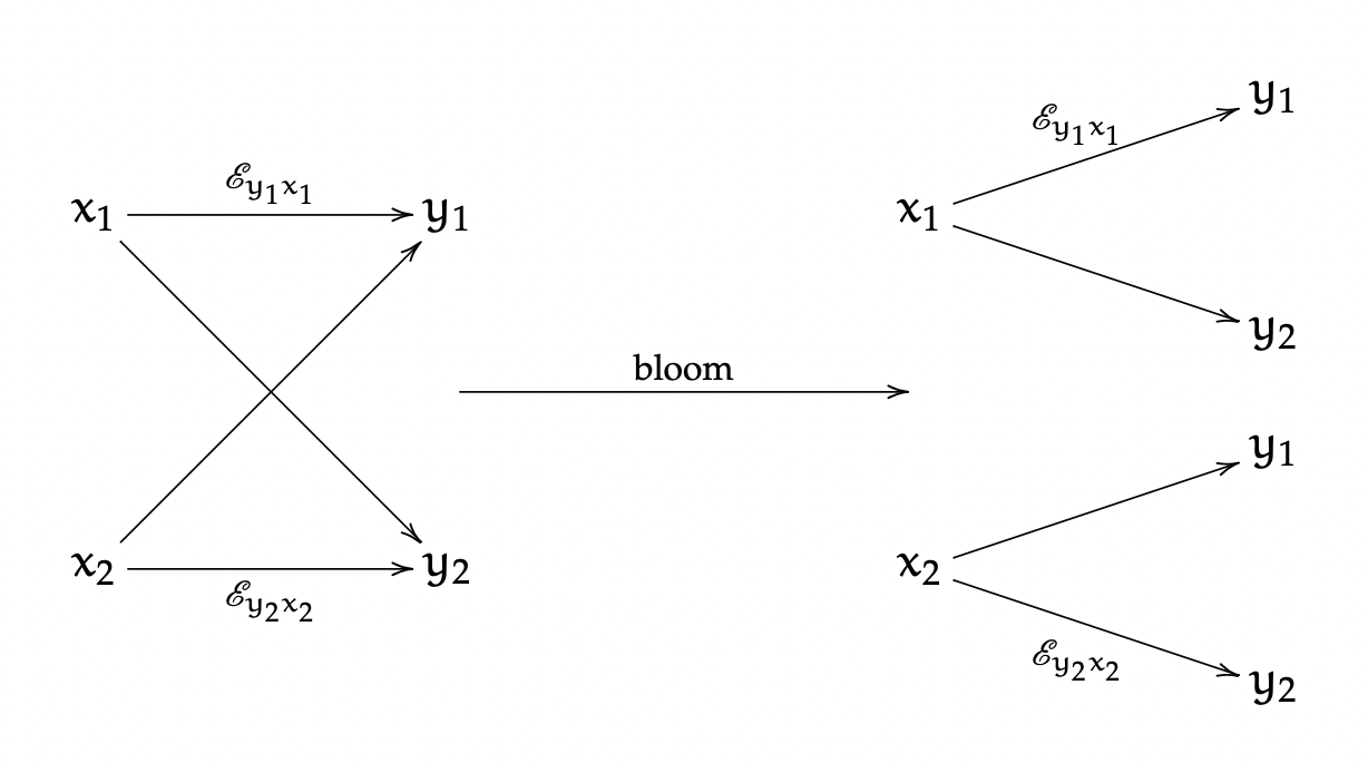
Figure 1: The bloom map "opens up" the classical channel $\mathscr{E}$.

Remark 3.5.

Given a pair of finite sets $(X,Y)$ and a classical process $(\rho,\mathscr{E})\in\mathscr{P}({{\mathbb{C}}}^{X},{{\mathbb{C}}}^{Y})$, if we identify $\mathscr{E}_{yx}$ with conditional probabilities $\mathbb{P}(y|x)$, $\rho\in\mathcal{S}({{\mathbb{C}}}^{X})$ with a probability distribution $\mathbb{P}(x)$ on $X$, and $\operatorname{\rotatebox[origin={c}]{180.0}{$!$}}_{\mathscr{E}}(\rho)$ with a joint probability distribution $\mathbb{P}(x,y)$ on $X\times Y$, then the equation

$$\operatorname{\rotatebox[origin={c}]{180.0}{$!$}}_{\mathscr{E}}(\rho)_{(x,y)}=\rho_{x}\mathscr{E}_{yx}$$

may be re-written as

$$\mathbb{P}(x,y)=\mathbb{P}(x)\mathbb{P}(y|x),$$ (3.6)

which is the classical equation relating a joint distribution with a conditional distribution and a prior. As such, Proposition 3.2 may be interpreted as saying that the joint distribution $\mathbb{P}(x,y)$ associated with a classical process $(\rho,\mathscr{E})\in\mathscr{P}({{\mathbb{C}}}^{X},{{\mathbb{C}}}^{Y})$ arises as an intermediary step in a canonical factorization $\mathscr{E}=\text{tr}_{X}\circ\operatorname{\rotatebox[origin={c}]{180.0}{$!$}}_{\mathscr{E}}$ of the associated channel. This observation will be crucial for generalizing joint distributions to the quantum domain.

Next we show that in the classical domain, joint distributions are in a bijective correspondence with classical processes.

Notation 3.7.

Given a pair $(X,Y)$ of finite sets, let $\mathcal{S}^{X}_{+}({{\mathbb{C}}}^{X}\otimes{{\mathbb{C}}}^{Y})\subset\mathcal{S}({{\mathbb{C}}}^{X}\otimes{{\mathbb{C}}}^{Y})$ denote the subset given by

$$\mathcal{S}^{X}_{+}({{\mathbb{C}}}^{X}\otimes{{\mathbb{C}}}^{Y})=\left\{\tau\in\mathcal{S}({{\mathbb{C}}}^{X}\otimes{{\mathbb{C}}}^{Y})\hskip 2.84526pt|\hskip 2.84526pt\text{$\text{tr}_{Y}(\tau)$ is invertible}\right\}.$$

Proposition 3.8.

Let $(X,Y)$ be a pair of finite sets, and let

$$\mathfrak{S}:\mathscr{P}_{+}({{\mathbb{C}}}^{X},{{\mathbb{C}}}^{Y})\longrightarrow\mathcal{S}^{X}_{+}({{\mathbb{C}}}^{X}\otimes{{\mathbb{C}}}^{Y})$$

be the map given by $\mathfrak{S}(\rho,\mathscr{E})=\operatorname{\rotatebox[origin={c}]{180.0}{$!$}}_{\mathscr{E}}(\rho)$. Then $\mathfrak{S}$ is a bijection, whose inverse is determined by the condition

$$\mathfrak{S}^{-1}(\tau)=(\rho,\mathscr{E})\implies\mathscr{E}_{yx}=\frac{\tau_{(x,y)}}{\rho_{x}}\quad\quad\forall(x,y)\in X\times Y.$$

Proof.

Let $(X,Y)$ be a pair of finite sets, and let $\mathfrak{C}:\mathcal{S}^{X}_{+}({{\mathbb{C}}}^{X}\otimes{{\mathbb{C}}}^{Y})\longrightarrow\mathscr{P}_{+}({{\mathbb{C}}}^{X},{{\mathbb{C}}}^{Y})$ be the map uniquely determined by the condition

$$\mathfrak{C}(\tau)=(\rho,\mathscr{E})\implies\mathscr{E}_{yx}=\frac{\tau_{(x,y)}}{\rho_{x}}\quad\quad\forall(x,y)\in X\times Y.$$

We will show $\mathfrak{C}\circ\mathfrak{S}=\text{id}$ and $\mathfrak{S}\circ\mathfrak{C}=\text{id}$. For the former case, let $(\rho,\mathscr{E})\in\mathscr{P}_{+}({{\mathbb{C}}}^{X},{{\mathbb{C}}}^{Y})$, and let $(\widetilde{\rho},\widetilde{\mathscr{E}})=\mathfrak{C}\left(\mathfrak{S}(\rho,\mathscr{E})\right)$. By the definition of $\mathfrak{C}$ we have

$$\mathfrak{C}(\tau)=(\rho,\mathscr{E}) \implies \mathscr{E}_{yx}=\frac{\tau_{(x,y)}}{\rho_{x}}\quad\quad\hskip 75.39963pt\forall(x,y)\in X\times Y$$

$$\implies \sum_{y\in Y}\tau_{(x,y)}=\sum_{y\in Y}\rho_{x}\mathscr{E}_{yx}=\rho_{x}\quad\quad\forall x\in X$$

$$\implies \text{tr}_{Y}(\tau)=\rho,$$

thus

$$\widetilde{\rho}=\text{tr}_{Y}\left(\mathfrak{S}(\rho,\mathscr{E})\right)=\text{tr}_{Y}\left(\operatorname{\rotatebox[origin={c}]{180.0}{$!$}}_{\mathscr{E}}(\rho)\right)=\rho.$$

Moreover, by definition of $\mathfrak{C}$, for all $(x,y)\in X\times Y$ we have

$$\widetilde{\mathscr{E}}_{yx}=\frac{\operatorname{\rotatebox[origin={c}]{180.0}{$!$}}_{\mathscr{E}}(\rho)_{(x,y)}}{\widetilde{\rho}_{x}}=\frac{\rho_{x}\mathscr{E}_{yx}}{\rho_{x}}=\mathscr{E}_{yx}\implies\widetilde{\mathscr{E}}=\mathscr{E},$$

thus $\mathfrak{C}\circ\mathfrak{S}=\text{id}$.

Now let $\tau\in\mathcal{S}^{X}_{+}({{\mathbb{C}}}^{X}\otimes{{\mathbb{C}}}^{Y})$, let $(\rho,\mathscr{E})=\mathfrak{C}(\tau)$, and let $\widetilde{\tau}=\mathfrak{S}(\mathfrak{C}(\tau))$. Then for all $(x,y)\in X\times Y$ we have

$$\widetilde{\tau}_{(x,y)}=\mathfrak{S}(\rho,\mathscr{E})_{(x,y)}=\rho_{x}\mathscr{E}_{yx}=\rho_{x}\left(\frac{\tau_{(x,y)}}{\rho_{x}}\right)=\tau_{(x,y)}\implies\widetilde{\tau}=\tau,$$

thus $\mathfrak{S}\circ\mathfrak{C}=\text{id}$, as desired. ∎

Remark 3.9.

In light of Proposition 3.8, it follows that a state $\tau\in\mathcal{S}^{X}_{+}({{\mathbb{C}}}^{X}\otimes{{\mathbb{C}}}^{Y})$ may either be viewed as a joint distribution associated with two space-like separated random variables $X$ and $Y$ occurring in parallel, or as a state over time $\operatorname{\rotatebox[origin={c}]{180.0}{$!$}}_{\mathscr{E}}(\rho)$ associated with the process $(\rho,\mathscr{E})=\mathfrak{C}(\tau)\in\mathscr{P}_{+}({{\mathbb{C}}}^{X},{{\mathbb{C}}}^{Y})$. These two equivalent viewpoints are what we refer to as the static-dynamic duality for classical joint states in $\mathcal{S}^{X}_{+}({{\mathbb{C}}}^{X}\otimes{{\mathbb{C}}}^{Y})$. Another way to think of the static-dynamic duality for classical joint states, is that classical probability does not distinguish between temporal correlations and spatial correlations, revealing a certain symmetry between space and time for classical random variables. For quantum systems however it turns out that such a symmetry between space and time does not exist, as there exists quantum processes for which temporal correlations may not be viewed as spatial correlations and vice-versa [FJV15]. As such, the static-dynamic duality for classical joint states does not generalize to the quantum domain, and we will see that this is manifested in the fact that quantum states over time are not positive in general. This fact will play a crucial role in the general theory of states over time for quantum processes.

In the next proposition, we show how the state over time $\operatorname{\rotatebox[origin={c}]{180.0}{$!$}}_{\mathscr{E}}(\rho)$ associated with a classical process $(\rho,\mathscr{E})\in\mathscr{P}({{\mathbb{C}}}^{X},{{\mathbb{C}}}^{Y})$ may be re-written in a way that is valid for all quantum processes, which we will use in the next section for a quantum generalization of states over time.

Proposition 3.10.

Let $(X,Y)$ be a pair of finite sets, and let $\mathscr{E}\in\mathbb{CPTP}({{\mathbb{C}}}^{X},{{\mathbb{C}}}^{Y})$. Then

$$\operatorname{\rotatebox[origin={c}]{180.0}{$!$}}_{\mathscr{E}}(\rho)=(\rho\otimes\mathds{1})\mathscr{J}[\mathscr{E}]$$ (3.11)

for all $\rho\in{{\mathbb{C}}}^{X}$. In particular, if $\rho\in\mathcal{S}({{\mathbb{C}}}^{X})$, then $(\rho\otimes\mathds{1})\mathscr{J}[\mathscr{E}]$ is the state over time associated with the classical process $(\rho,\mathscr{E})$.

Proof.

Let $\mu:{{\mathbb{C}}}^{X}\otimes{{\mathbb{C}}}^{X}\longrightarrow{{\mathbb{C}}}^{X}$ denote the multiplication map. From the definition of the Hilbert-Schmidt dual we have

$$\mu^{*}(\mathds{1})=\sum_{x\in X}\delta_{x}\otimes\delta_{x}\hskip 0.7113pt,$$

thus

$$\mathscr{J}[\mathscr{E}] = \left(\text{id}_{{{\mathbb{C}}}^{X}}\otimes\mathscr{E}\right)(\mu^{*}(\mathds{1}))=\left(\text{id}_{{{\mathbb{C}}}^{X}}\otimes\mathscr{E}\right)\left(\sum_{x\in X}\delta_{x}\otimes\delta_{x}\right)=\sum_{x\in X}\delta_{x}\otimes\mathscr{E}(\delta_{x})$$

$$= \sum_{x\in X}\delta_{x}\otimes\left(\sum_{y\in Y}\mathscr{E}_{yx}\delta_{y}\right)=\sum_{(x,y)\in X\times Y}\mathscr{E}_{yx}(\delta_{x}\otimes\delta_{y}).$$

And since for all $\rho\in{{\mathbb{C}}}^{X}$ we have

$$\rho\otimes\mathds{1}=\left(\sum_{x\in X}\rho_{x}\delta_{x}\right)\otimes\left(\sum_{y\in Y}\delta_{y}\right)=\sum_{(x,y)\in X\times Y}\rho_{x}(\delta_{x}\otimes\delta_{y}),$$

it follows that

$$(\rho\otimes\mathds{1})\mathscr{J}[\mathscr{E}] = \left(\sum_{(x,y)\in X\times Y}\rho_{x}(\delta_{x}\otimes\delta_{y})\right)\left(\sum_{(x,y)\in X\times Y}\mathscr{E}_{yx}(\delta_{x}\otimes\delta_{y})\right)$$

$$= \sum_{(x,y)\in X\times Y}\rho_{x}\mathscr{E}_{yx}(\delta_{x}\otimes\delta_{y})$$

$$= \operatorname{\rotatebox[origin={c}]{180.0}{$!$}}_{\mathscr{E}}(\rho),$$

as desired. ∎

Remark 3.12.

While up to now the left-hand side of equation (3.11) is only defined for classical processes, the right-hand side is defined for any quantum process $(\rho,\mathscr{E})$. Moreover, since for classical processes we have $\left[\mathscr{J}[\mathscr{E}],(\rho\otimes\mathds{1})\right]=0$, the right-hand side of equation (3.11) coincides with

$$\lambda(\rho\otimes\mathds{1})\mathscr{J}[\mathscr{E}]+(1-\lambda)\mathscr{J}[\mathscr{E}](\rho\otimes\mathds{1})$$ (3.13)

for all $\lambda\in{{\mathbb{C}}}$, which is also well-defined for any quantum process $(\rho,\mathscr{E})$. However when $\left[(\rho\otimes\mathds{1}),\mathscr{J}[\mathscr{E}]\right]\neq 0$ and $\lambda\neq 1$ the expression (3.13) is distinct from $(\rho\otimes\mathds{1})\mathscr{J}[\mathscr{E}]$, thus in the quantum domain, (3.13) yields a parametric family of states over time associated with a general quantum process $(\rho,\mathscr{E})$ which generalizes the classical state over time $\operatorname{\rotatebox[origin={c}]{180.0}{$!$}}_{\mathscr{E}}(\rho)$. Another crucial point, is that while the multi-matrix (3.13) is of unit trace for all $\lambda\in{{\mathbb{C}}}$, in the quantum domain it is rarely positive (even for $\lambda\in{{\mathbb{R}}}$), and is only guaranteed to be self-adjoint for $\lambda=1/2$. As such, when generalizing states over time to the quantum domain, we will relax the positivity condition and only require states over time to be self-adjoint elements of unit trace. In fact, as first pointed out in [FJV15], it is the negative eigenvalues of a quantum state over time which act as a witness to causal correlations which exist in the associated process, and are a feature of the theory rather than a defect.

4 In quantum bloom

The classical bloom map $\operatorname{\rotatebox[origin={c}]{180.0}{$!$}}_{\mathscr{E}}$ from Proposition 3.2 may be viewed as the output of a mapping that associates every pair $(X,Y)$ of finite sets with a function

$$\operatorname{\rotatebox[origin={c}]{180.0}{$!$}}_{(*)}:\mathbb{CPTP}({{\mathbb{C}}}^{X},{{\mathbb{C}}}^{Y})\longrightarrow\mathbb{CPTP}({{\mathbb{C}}}^{X},{{\mathbb{C}}}^{X}\otimes{{\mathbb{C}}}^{Y})$$ (4.1)

such that $\text{tr}_{X}\circ\operatorname{\rotatebox[origin={c}]{180.0}{$!$}}_{\mathscr{E}}=\mathscr{E}$ and $\text{tr}_{Y}\circ\operatorname{\rotatebox[origin={c}]{180.0}{$!$}}_{\mathscr{E}}=\mathrm{id}_{{{\mathbb{C}}}^{X}}$ for all $\mathscr{E}\in\mathbb{CPTP}({{\mathbb{C}}}^{X},{{\mathbb{C}}}^{Y})$. Moreover, the bloom map $\operatorname{\rotatebox[origin={c}]{180.0}{$!$}}_{(*)}$ naturally extends to a map on all of $\text{Hom}({{\mathbb{C}}}^{X},{{\mathbb{C}}}^{Y})$, which together with the partial trace provides a factorization system on $\text{Hom}({{\mathbb{C}}}^{X},{{\mathbb{C}}}^{Y})$ which yields the state over time $\operatorname{\rotatebox[origin={c}]{180.0}{$!$}}_{\mathscr{E}}(\rho)$ associated with every classical process $(\rho,\mathscr{E})\in\mathscr{P}({{\mathbb{C}}}^{X},{{\mathbb{C}}}^{Y})$. In this section, we extend the classical bloom map (4.1) to the quantum domain. Though there are various such extensions, the extension referred to as the symmetric bloom yields a state over time which is always self-adjoint, and will be the focus of our work.

Definition 4.2.

A bloom map associates every pair $(\mathcal{A},\mathcal{B})$ of multi-matrix algebras with a map $\operatorname{\rotatebox[origin={c}]{180.0}{$!$}}:\mathbb{TP}(\mathcal{A},\mathcal{B})\longrightarrow\mathbb{TP}(\mathcal{A},\mathcal{A}\otimes\mathcal{B})$ such that $\text{tr}_{\mathcal{A}}\circ\operatorname{\rotatebox[origin={c}]{180.0}{$!$}}(\mathscr{E})=\mathscr{E}$ and $\text{tr}_{\mathcal{B}}\circ\operatorname{\rotatebox[origin={c}]{180.0}{$!$}}(\mathscr{E})=\text{id}_{\mathcal{A}}$ for all $\mathscr{E}\in\mathbb{TP}(\mathcal{A},\mathcal{B})$.

Definition 4.3.

If $(\rho,\mathscr{E})\in\mathscr{P}(\mathcal{A},\mathcal{B})$ is a quantum process, and $\operatorname{\rotatebox[origin={c}]{180.0}{$!$}}$ is a bloom map, then $\operatorname{\rotatebox[origin={c}]{180.0}{$!$}}(\mathscr{E})(\rho)$ will be referred to as the state over time associated with the process $(\rho,\mathscr{E})$ and the bloom map $\operatorname{\rotatebox[origin={c}]{180.0}{$!$}}$, and will be denoted by $\operatorname{\rotatebox[origin={c}]{180.0}{$!$}}(\rho,\mathscr{E})$. The map on quantum processes given by

$$(\rho,\mathscr{E})\longmapsto\operatorname{\rotatebox[origin={c}]{180.0}{$!$}}(\rho,\mathscr{E})$$

will then be referred to as the state over time function associated with $\operatorname{\rotatebox[origin={c}]{180.0}{$!$}}$.

Definition 4.4.

Given a bloom map $\operatorname{\rotatebox[origin={c}]{180.0}{$!$}}$, the factorization $\mathscr{E}=\text{tr}_{\mathcal{A}}\circ\operatorname{\rotatebox[origin={c}]{180.0}{$!$}}(\mathscr{E})$ will be referred to as the bloom-shriek factorization of $\mathscr{E}\in\mathbb{TP}(\mathcal{A},\mathcal{B})$.

Remark 4.5.

An analogue of bloom-shriek factorization for free gs-monoidal categories appears in [fritz2023free] under the name bloom-circuitry factorization.

Example 4.6.

Let $(\mathcal{A},\mathcal{B})$ be a pair of multi-matrix algebras, and let

$$\operatorname{\rotatebox[origin={c}]{180.0}{$!$}}:\mathbb{TP}(\mathcal{A},\mathcal{B})\longrightarrow\mathbb{TP}(\mathcal{A},\mathcal{A}\otimes\mathcal{B})$$

be the map given by $\operatorname{\rotatebox[origin={c}]{180.0}{$!$}}(\mathscr{E})(\rho)=(\rho\otimes\mathds{1})\mathscr{J}[\mathscr{E}]$. When $\mathcal{A}$ is a matrix algebra it was shown in [PaRuBayes] that $\mu_{\mathcal{A}}^{*}(\mathds{1})=\sum_{i,j}E_{ij}\otimes E_{ji}$, where $E_{ij}$ are the matrix units in $\mathcal{A}$. We then have

$$\operatorname{\rotatebox[origin={c}]{180.0}{$!$}}(\mathscr{E})(\rho) = (\rho\otimes\mathds{1})\mathscr{J}[\mathscr{E}]=(\rho\otimes\mathds{1})(\mathrm{id}_{\mathcal{A}}\otimes\mathscr{E})\left(\mu_{\mathcal{A}}^{*}(\mathds{1})\right)$$

$$= (\rho\otimes\mathds{1})(\mathrm{id}_{\mathcal{A}}\otimes\mathscr{E})\left(\sum_{i,j}E_{ij}\otimes E_{ji}\right)=(\rho\otimes\mathds{1})\left(\sum_{i,j}E_{ij}\otimes\mathscr{E}(E_{ji})\right)$$

$$= \sum_{i,j}\rho E_{ij}\otimes\mathscr{E}(E_{ji}),$$

from which it follows that

$$\text{tr}_{\mathcal{A}}\left(\operatorname{\rotatebox[origin={c}]{180.0}{$!$}}(\mathscr{E})(\rho)\right)=\sum_{i,j}\text{tr}(\rho E_{ij})\mathscr{E}(E_{ji})=\sum_{i,j}\rho_{ji}\mathscr{E}(E_{ji})=\mathscr{E}(\rho),$$

and

$$\text{tr}_{\mathcal{B}}\left(\operatorname{\rotatebox[origin={c}]{180.0}{$!$}}(\mathscr{E})(\rho)\right)=\sum_{i,j}\text{tr}(\mathscr{E}(E_{ji}))\rho E_{ij}=\sum_{i,j}\delta_{ji}\rho E_{ij}=\sum_{i}\rho E_{ii}=\rho,$$

thus $\operatorname{\rotatebox[origin={c}]{180.0}{$!$}}$ defines a bloom map in this case. When $\mathcal{A}=\bigoplus_{x\in X}\mathbb{M}_{m_{x}}$ and $\mathcal{B}=\bigoplus_{y\in Y}\mathbb{M}_{n_{y}}$ are both multi-matrix algebras, then

$$\rho=\bigoplus_{x\in X}\rho_{x}\quad\&\quad\mathscr{J}[\mathscr{E}]=\bigoplus_{(x,y)\in X\times Y}\mathscr{J}[\mathscr{E}_{yx}],$$

where $\mathscr{E}_{yx}$ are the component functions of $\mathscr{E}\in\text{Hom}(\mathcal{A},\mathcal{B})$. We then have

$$\operatorname{\rotatebox[origin={c}]{180.0}{$!$}}(\mathscr{E})(\rho)=(\rho\otimes\mathds{1})\mathscr{J}[\mathscr{E}]=\bigoplus_{(x,y)\in X\times Y}(\rho_{x}\otimes\mathds{1})\mathscr{J}[\mathscr{E}_{yx}],$$

thus the above arguments in the case when $\mathcal{A}$ is a matrix algebra may be applied component-wise to deduce $\text{tr}_{\mathcal{A}}\circ\operatorname{\rotatebox[origin={c}]{180.0}{$!$}}(\mathscr{E})=\mathscr{E}$ and $\text{tr}_{\mathcal{B}}\circ\operatorname{\rotatebox[origin={c}]{180.0}{$!$}}(\mathscr{E})=\text{id}_{\mathcal{A}}$, thus $\operatorname{\rotatebox[origin={c}]{180.0}{$!$}}$ defines a bloom map. Moreover, it follows from Proposition 3.10 that this bloom map recovers the classical state over time $\operatorname{\rotatebox[origin={c}]{180.0}{$!$}}_{\mathscr{E}}(\rho)$ associated with classical processes $(\rho,\mathscr{E})\in\mathscr{P}({{\mathbb{C}}}^{X},{{\mathbb{C}}}^{Y})$.

In light of the previous example, the following definition provides three examples of bloom maps.

Definition 4.7.

Let $(\mathcal{A},\mathcal{B})$ be a pair of multi-matrix algebras.

• The right bloom is the map $\operatorname{\rotatebox[origin={c}]{180.0}{$!$}}_{R}:\mathbb{TP}(\mathcal{A},\mathcal{B})\longrightarrow\mathbb{TP}(\mathcal{A},\mathcal{A}\otimes\mathcal{B})$ given by $\mathscr{E}\longmapsto\operatorname{\rotatebox[origin={c}]{180.0}{$!$}}_{R}(\mathscr{E})$, where

  $$\operatorname{\rotatebox[origin={c}]{180.0}{$!$}}_{R}(\mathscr{E})(\rho)=(\rho\otimes\mathds{1})\mathscr{J}[\mathscr{E}]$$

  for all $\rho\in\mathcal{A}$.

• The left bloom is the map $\operatorname{\rotatebox[origin={c}]{180.0}{$!$}}_{L}:\mathbb{TP}(\mathcal{A},\mathcal{B})\longrightarrow\mathbb{TP}(\mathcal{A},\mathcal{A}\otimes\mathcal{B})$ given by $\mathscr{E}\longmapsto\operatorname{\rotatebox[origin={c}]{180.0}{$!$}}_{L}(\mathscr{E})$, where

  $$\operatorname{\rotatebox[origin={c}]{180.0}{$!$}}_{L}(\mathscr{E})(\rho)=\mathscr{J}[\mathscr{E}](\rho\otimes\mathds{1})$$

  for all $\rho\in\mathcal{A}$.

• The symmetric bloom is the map $\text{\Yinyang}:\mathbb{TP}(\mathcal{A},\mathcal{B})\longrightarrow\mathbb{TP}(\mathcal{A},\mathcal{A}\otimes\mathcal{B})$ given by $\mathscr{E}\longmapsto\text{\Yinyang}(\mathscr{E})$, where

  $$\text{\Yinyang}(\mathscr{E})(\rho)=\frac{1}{2}\left((\rho\otimes\mathds{1})\mathscr{J}[\mathscr{E}]+\mathscr{J}[\mathscr{E}](\rho\otimes\mathds{1})\right)$$

  for all $\rho\in\mathcal{A}$.

Remark 4.8.

The symmetric bloom was introduced in [FuPa22], where it was proved that the associated state over time function $(\rho,\mathscr{E})\longmapsto\text{\Yinyang}(\rho,\mathscr{E}):=\text{\Yinyang}(\mathscr{E})(\rho)$ satisfies a list of axioms set forth in [HHPBS17]. The list of axioms include hermiticity of $\text{\Yinyang}(\rho,\mathscr{E})$, bilinearity of $\text{\Yinyang}(*,*)$, a classical limit axiom, and an associativity axiom which ensures that extends in a well-defined way to $n$-step processes $(\rho,\mathscr{E}_{1},...,\mathscr{E}_{n})$. In a later work we will prove that the symmetric bloom is in fact the only state over time function satisfying the aforementioned list of axioms.

The following statement yields an important property of the symmetric bloom which will be useful for our purposes.

Proposition 4.9.

The $(\mathcal{A},\mathcal{B})$ be a pair of multi-matrix algebras, and let $\mathscr{E}\in\mathbb{TP}(\mathcal{A},\mathcal{B})$. Then the following statements are equivalent.

1. $\mathscr{E}$ is ${\dagger}$-preserving.

2. $\mathscr{J}[\mathscr{E}]$ is self-adjoint.

3. $\emph{\Yinyang}(\mathscr{E})$ is ${\dagger}$-preserving.

Proof.

We prove the statement in the case of matrix algebras.

i$\implies$ ii: Let $\mu:\mathcal{A}\otimes\mathcal{A}\longrightarrow\mathcal{A}$ denote the multiplication map. It follows from [PaRuBayes] that

$$\mu^{*}(\mathds{1})=\sum_{i,j}E_{ij}\otimes E_{ji},$$

thus

$$\mathscr{J}[\mathscr{E}]=\left(\mathrm{id}_{\mathcal{A}}\otimes\mathscr{E}\right)\mu^{*}(\mathds{1})=\left(\mathrm{id}_{\mathcal{A}}\otimes\mathscr{E}\right)\left(\sum_{i,j}E_{ij}\otimes E_{ji}\right)=\sum_{i,j}E_{ij}\otimes\mathscr{E}(E_{ji}).$$

We then have

$$\mathscr{J}[\mathscr{E}]^{{\dagger}} = \left(\sum_{i,j}E_{ij}\otimes\mathscr{E}(E_{ji})\right)^{{\dagger}}=\sum_{i,j}E_{ij}^{{\dagger}}\otimes\mathscr{E}(E_{ji})^{{\dagger}}$$

$$= \sum_{i,j}E_{ji}\otimes\mathscr{E}(E_{ji}^{{\dagger}})=\sum_{i,j}E_{ji}\otimes\mathscr{E}(E_{ij})$$

$$= \mathscr{J}[\mathscr{E}],$$

as desired.

ii$\implies$ iii: Let $\rho\in\mathcal{A}$. Then

$$\text{\Yinyang}(\mathscr{E})(\rho)^{{\dagger}} = \frac{1}{2}\left((\rho\otimes\mathds{1})\mathscr{J}[\mathscr{E}]+\mathscr{J}[\mathscr{E}](\rho\otimes\mathds{1})\right)^{{\dagger}}$$

$$= \frac{1}{2}\left(\mathscr{J}[\mathscr{E}]^{{\dagger}}(\rho\otimes\mathds{1})^{{\dagger}}+(\rho\otimes\mathds{1})^{{\dagger}}\mathscr{J}[\mathscr{E}]^{{\dagger}}\right)$$

$$= \frac{1}{2}\left(\mathscr{J}[\mathscr{E}](\rho^{{\dagger}}\otimes\mathds{1})+(\rho^{{\dagger}}\otimes\mathds{1})\mathscr{J}[\mathscr{E}]\right)$$

$$= \text{\Yinyang}(\mathscr{E})(\rho^{{\dagger}}),$$

thus $\text{\Yinyang}(\mathscr{E})$ is ${\dagger}$-preserving.

iii$\implies$ i: Since

$$\text{tr}_{\mathcal{A}}(A\otimes B)^{{\dagger}}=\left(\text{tr}(A)B\right)^{{\dagger}}=\overline{\text{tr}(A)}B^{{\dagger}}=\text{tr}(A^{{\dagger}})B^{{\dagger}}=\text{tr}_{\mathcal{A}}(A^{{\dagger}}\otimes B^{{\dagger}})=\text{tr}_{\mathcal{A}}\left((A\otimes B)^{{\dagger}}\right),$$

it follows that $\text{tr}_{\mathcal{A}}$ is ${\dagger}$-preserving. For all $\rho\in A$ we then have

$$\mathscr{E}(\rho)^{{\dagger}}=(\text{tr}_{\mathcal{A}}\circ\text{\Yinyang}(\mathscr{E}))(\rho)^{{\dagger}}=\text{tr}_{\mathcal{A}}\left(\text{\Yinyang}(\mathscr{E})(\rho)\right)^{{\dagger}}=\text{tr}_{\mathcal{A}}\left(\text{\Yinyang}(\mathscr{E})(\rho)^{{\dagger}}\right)=\text{tr}_{\mathcal{A}}\left(\text{\Yinyang}(\mathscr{E})(\rho^{{\dagger}})\right)=\mathscr{E}(\rho^{{\dagger}}),$$

as desired. ∎

Definition 4.10.

A bloom map $\operatorname{\rotatebox[origin={c}]{180.0}{$!$}}$ is said to be

• classically reducible if and only if $\left[(\rho\otimes\mathds{1}),\mathscr{J}[\mathscr{E}]\right]=0\implies\operatorname{\rotatebox[origin={c}]{180.0}{$!$}}(\mathscr{E})(\rho)=(\rho\otimes\mathds{1})\mathscr{J}[\mathscr{E}]$.

• hermitian if and only if $\operatorname{\rotatebox[origin={c}]{180.0}{$!$}}(\mathscr{E})$ is ${\dagger}$-preserving whenever $\mathscr{E}$ is ${\dagger}$-preserving.

Remark 4.11.

By Proposition 4.9 it follows that the symmetric bloom is hermitian, and it follows directly from its definition that the symmetric bloom is classically reducible. These are two key properties one should expect from a quantum bloom map if it is to be viewed as generalization of the classical bloom. While we have reason to believe that the symmetric bloom is the only bloom map which is both hermitian and classically reducible, we have yet to prove such a result.

We now generalize Proposition 3.8 using the symmetric bloom. In particular, given a pseudo-density operator on $\tau\in\mathcal{A}\otimes\mathcal{B}$, we derive an explicit formula for a process $(\rho,\mathscr{E})$ such that $\tau=\text{\Yinyang}(\rho,\mathscr{E})$. For this, we recall that $\mathscr{T}(\mathcal{A}\otimes\mathcal{B})$ denotes the set of pseudo-density operators with respect to the tensor factorization $\mathcal{A}_{0}=\mathcal{A}\otimes\mathcal{B}$ (see Definition 2.20).

Lemma 4.12.

Let $\tau\in\mathscr{T}(\mathcal{A}\otimes\mathcal{B})$ be such that $\emph{tr}_{\mathcal{B}}(\tau)$ is invertible. Then there exists a unique element $X_{\tau}\in\mathcal{A}\otimes\mathcal{B}$ such that

$$(\emph{tr}_{\mathcal{B}}(\tau)\otimes\mathds{1})X_{\tau}+X_{\tau}(\emph{tr}_{\mathcal{B}}(\tau)\otimes\mathds{1})=2\tau.$$ (4.13)

Proof.

We prove the statement in the case of matrix algebras, where we will use the fact from linear algebra that if $A,B,C\in\mathbb{M}_{n}$, then the Sylvester equation $AX+XB=C$ has a unique solution $X\in\mathbb{M}_{n}$ if and only if $A$ and $-B$ have disjoint spectrums. So let $\tau\in\mathscr{T}(\mathcal{A}\otimes\mathcal{B})$ be such that $\text{tr}_{\mathcal{B}}(\tau)$ is invertible. Since $\text{tr}_{\mathcal{B}}(\tau)$ is a state which is invertible, it follows that the eigenvalues of $\text{tr}_{\mathcal{B}}(\tau)$ are strictly positive, thus the spectrums of $\text{tr}_{\mathcal{B}}(\tau)\otimes\mathds{1}$ and $-(\text{tr}_{\mathcal{B}}(\tau)\otimes\mathds{1})$ are disjoint. It then follows that the Sylvester equation

$$(\text{tr}_{\mathcal{B}}(\tau)\otimes\mathds{1})X+X(\text{tr}_{\mathcal{B}}(\tau)\otimes\mathds{1})=2\tau$$

has a unique solution $X_{\tau}\in\mathcal{A}\otimes\mathcal{B}$, thus proving the statement. ∎

Notation 4.14.

Given a pair $(\mathcal{A},\mathcal{B})$ of multi-matrix algebras, we let

$$\mathscr{T}_{*}(\mathcal{A}\otimes\mathcal{B})\subset\mathscr{T}^{\mathcal{A}}_{+}(\mathcal{A}\otimes\mathcal{B})\subset\mathscr{T}(\mathcal{A}\otimes\mathcal{B})$$ (4.15)

denote the subsets given by

$$\mathscr{T}^{\mathcal{A}}_{+}(\mathcal{A}\otimes\mathcal{B})=\left\{\tau\in\mathscr{T}(\mathcal{A}\otimes\mathcal{B})\hskip 2.84526pt|\hskip 2.84526pt\text{tr}_{\mathcal{B}}(\tau)\hskip 2.84526pt\text{is invertible}\right\},$$

and

$$\mathscr{T}_{*}(\mathcal{A}\otimes\mathcal{B})=\left\{\tau\in\mathscr{T}^{\mathcal{A}}_{+}(\mathcal{A}\otimes\mathcal{B})\hskip 2.84526pt|\hskip 2.84526pt\mathscr{J}^{-1}(X_{\tau})\in\mathbb{CPTP}(\mathcal{A},\mathcal{B})\right\},$$

where $X_{\tau}\in\mathcal{A}\otimes\mathcal{B}$ is the unique element satisfying (4.13).

Lemma 4.16.

Let $(\mathcal{A},\mathcal{B})$ be a pair of multi-matrix algebras. Then $\text{\Yinyang}(\rho,\mathscr{E})\in\mathscr{T}_{*}(\mathcal{A}\otimes\mathcal{B})$ for all $(\rho,\mathscr{E})\in\mathscr{P}_{+}(\mathcal{A},\mathcal{B})$.

Proof.

Let $(\rho,\mathscr{E})\in\mathscr{P}_{+}(\mathcal{A},\mathcal{B})$ and let $\tau=\text{\Yinyang}(\rho,\mathscr{E})$. To show $\tau\in\mathscr{T}_{*}(\mathcal{A}\otimes\mathcal{B})$ we need to show that $\tau$ is a pseudo-density operator such that $\text{tr}_{\mathcal{B}}(\tau)$ is invertible and $\mathscr{J}^{-1}(X_{\tau})$ is CPTP. To show $\tau$ is a pseuso-density operator we first show $\tau$ is self-adjoint. Now since $\mathscr{E}$ is CPTP it is ${\dagger}$-preserving thus $\text{\Yinyang}(\mathscr{E})$ is ${\dagger}$-preserving by Proposition 4.9. We then have

$$\tau^{{\dagger}}=\text{\Yinyang}(\rho,\mathscr{E})^{{\dagger}}=\text{\Yinyang}(\mathscr{E})(\rho)^{{\dagger}}=\text{\Yinyang}(\mathscr{E})(\rho^{{\dagger}})=\text{\Yinyang}(\mathscr{E})(\rho)=\tau,$$

thus $\tau$ is self-adjoint. And since the marginals of $\tau$ are $\rho$ and $\mathscr{E}(\rho)$ with $\rho$ invertible (since $(\rho,\mathscr{E})\in\mathscr{P}_{+}(\mathcal{A},\mathcal{B})$), it follows that $\tau\in\mathscr{T}^{\mathcal{A}}_{+}(\mathcal{A}\otimes\mathcal{B})$. Moreover, since $\rho=\text{tr}_{\mathcal{B}}(\tau)$ and

$$\tau=\frac{1}{2}\left((\rho\otimes\mathds{1})\mathscr{J}[\mathscr{E}]+\mathscr{J}[\mathscr{E}](\rho\otimes\mathds{1})\right),$$

it follows that $X_{\tau}=\mathscr{J}[\mathscr{E}]$ and $\mathscr{J}^{-1}(X_{\tau})=\mathscr{E}\in\mathbb{CPTP}(\mathcal{A},\mathcal{B})$, thus $\tau\in\mathscr{T}_{*}(\mathcal{A}\otimes\mathcal{B})$, as desired. ∎

Theorem 4.17.

Let $(\mathcal{A},\mathcal{B})$ be a pair of multi-matrix algebras, and let $\mathfrak{S}:\mathscr{P}_{+}(\mathcal{A},\mathcal{B})\longrightarrow\mathscr{T}_{*}(\mathcal{A}\otimes\mathcal{B})$ be the map given by $\mathfrak{S}(\rho,\mathscr{E})=\text{\Yinyang}(\rho,\mathscr{E})$. Then $\mathfrak{S}$ is a bijection, whose inverse is given by

$$\mathfrak{S}^{-1}(\tau)=\left(\emph{tr}_{\mathcal{B}}(\tau),\mathscr{J}^{-1}(X_{\tau})\right),$$ (4.18)

where $X_{\tau}\in\mathcal{A}\otimes\mathcal{B}$ is the unique element satisfying (4.13).

Proof.

Let $\mathfrak{C}:\mathscr{T}_{*}(\mathcal{A}\otimes\mathcal{B})\longrightarrow\mathscr{P}_{+}(\mathcal{A},\mathcal{B})$ be the map given by $\mathfrak{C}(\tau)=(\text{tr}_{\mathcal{B}}(\tau),\mathscr{J}^{-1}(X_{\tau}))$. We now show $\mathfrak{C}\circ\mathfrak{S}=\mathrm{id}$ and $\mathfrak{S}\circ\mathfrak{C}=\mathrm{id}$. So let $(\rho,\mathscr{E})\in\mathscr{P}_{+}(\mathcal{A},\mathcal{B})$ and let $\tau=\mathfrak{S}(\rho,\mathscr{E})$, so that $\rho=\text{tr}_{\mathcal{B}}(\tau)$ and

$$\tau=\frac{1}{2}\left((\rho\otimes\mathds{1})\mathscr{J}[\mathscr{E}]+\mathscr{J}[\mathscr{E}](\rho\otimes\mathds{1})\right)\implies\mathscr{J}[\mathscr{E}]=X_{\tau}\implies\mathscr{E}=\mathscr{J}^{-1}(X_{\tau}).$$

We then have

$$(\mathfrak{C}\circ\mathfrak{S})(\rho,\mathscr{E})=\mathfrak{C}(\tau)=(\text{tr}_{\mathcal{B}}(\tau),\mathscr{J}^{-1}(X_{\tau}))=(\rho,\mathscr{E}),$$

thus $\mathfrak{C}\circ\mathfrak{S}=\mathrm{id}$. Now let $\tau\in\mathscr{T}_{*}(\mathcal{A}\otimes\mathcal{B})$, so that

$$\frac{1}{2}\left(\text{tr}_{\mathcal{B}}(\tau)\otimes\mathds{1})X_{\tau}+X_{\tau}(\text{tr}_{\mathcal{B}}(\tau)\otimes\mathds{1}\right)=\tau.$$

We then have

$$(\mathfrak{S}\circ\mathfrak{C})(\tau) = \mathfrak{S}\left(\mathfrak{C}(\tau)\right)$$

$$= \mathfrak{S}(\text{tr}_{\mathcal{B}}(\tau),\mathscr{J}^{-1}(X_{\tau}))$$

$$= \frac{1}{2}\left((\text{tr}_{\mathcal{B}}(\tau)\otimes\mathds{1})\mathscr{J}[\mathscr{J}^{-1}(X_{\tau})]+\mathscr{J}[\mathscr{J}^{-1}(X_{\tau})](\text{tr}_{\mathcal{B}}(\tau)\otimes\mathds{1})\right)$$

$$= \frac{1}{2}\left(\text{tr}_{\mathcal{B}}(\tau)\otimes\mathds{1})X_{\tau}+X_{\tau}(\text{tr}_{\mathcal{B}}(\tau)\otimes\mathds{1}\right)$$

$$= \tau,$$

thus $\mathfrak{S}\circ\mathfrak{C}=\mathrm{id}$, as desired. ∎

5 Blooming 2-chains

Our next goal is to extend bloom maps to $n$-chains, but first we need to consider the case $n=2$. In this section we will show is that if a bloom map satisfies an associativity condition on $2$-chains, then it naturally extends to a unique bloom map on $2$-chains. We then show that the right bloom, left bloom and symmetric bloom are all associative, and as such, yield well-defined state over time functions for 2-step processes. In such a case we also prove an explicit formula for the symmetric bloom state over time function, and show that is satisfies a certain compositionality property. This will provide us with the mathematical foundation for using bloom maps to define explicit states over time associated with the dynamics of $n$-step quantum processes for all $n>0$.

Definition 5.1.

Given a triple $(\mathcal{A},\mathcal{B},\mathcal{C})$ of multi-matrix algebras, a $2$-chain consists of a pair $(\mathscr{E},\mathscr{F})\in\mathbb{TP}(\mathcal{A},\mathcal{B})\times\mathbb{TP}(\mathcal{B},\mathcal{C})$. The set of all such $2$-chains will be denoted by $\mathbb{TP}(\mathcal{A},\mathcal{B},\mathcal{C})$.

Example 5.2 (Blooming 2-chains).

Let $\mathcal{A}\overset{\mathscr{E}}{\longrightarrow}\mathcal{B}\overset{\mathscr{F}}{\longrightarrow}\mathcal{C}$ be a 2-chain, let $\operatorname{\rotatebox[origin={c}]{180.0}{$!$}}$ be a bloom map, and consider the following diagram.

(5.3)

Using only maps in the above diagram, there are two maps one may construct in $\mathbb{TP}(\mathcal{A},\mathcal{A}\otimes\mathcal{B}\otimes\mathcal{C})$, namely, $\operatorname{\rotatebox[origin={c}]{180.0}{$!$}}\left(\operatorname{\rotatebox[origin={c}]{180.0}{$!$}}(\mathscr{F})\circ\mathscr{E}\right)$ and $\operatorname{\rotatebox[origin={c}]{180.0}{$!$}}(\mathscr{F}\circ\text{tr})\circ\operatorname{\rotatebox[origin={c}]{180.0}{$!$}}(\mathscr{E})$. As the map $\operatorname{\rotatebox[origin={c}]{180.0}{$!$}}\left(\operatorname{\rotatebox[origin={c}]{180.0}{$!$}}(\mathscr{F})\circ\mathscr{E}\right)$ has codomain $\mathcal{A}\otimes(\mathcal{B}\otimes\mathcal{C})$ and the map $\operatorname{\rotatebox[origin={c}]{180.0}{$!$}}(\mathscr{F}\circ\text{tr})\circ\operatorname{\rotatebox[origin={c}]{180.0}{$!$}}(\mathscr{E})$ has codomain $(\mathcal{A}\otimes\mathcal{B})\otimes\mathcal{C}$, there is a bijection between 2-blooms constructed from the above diagram and parenthezations of the multi-matrix algebra $\mathcal{A}\otimes\mathcal{B}\otimes\mathcal{C}$. It is then a natural to question whether or not the two maps $\operatorname{\rotatebox[origin={c}]{180.0}{$!$}}\left(\operatorname{\rotatebox[origin={c}]{180.0}{$!$}}(\mathscr{F})\circ\mathscr{E}\right)$ and $\operatorname{\rotatebox[origin={c}]{180.0}{$!$}}(\mathscr{F}\circ\text{tr})\circ\operatorname{\rotatebox[origin={c}]{180.0}{$!$}}(\mathscr{E})$ are equal. If the two maps are in fact equal, then the bloom map $\operatorname{\rotatebox[origin={c}]{180.0}{$!$}}$ naturally extends to a unique bloom map on 2-chains. Such considerations then motivate the following definition.

Definition 5.4.

A bloom map $\operatorname{\rotatebox[origin={c}]{180.0}{$!$}}$ is said to be associative if and only if for every 2-chain

$$\mathcal{A}\overset{\mathscr{E}}{\longrightarrow}\mathcal{B}\overset{\mathscr{F}}{\longrightarrow}\mathcal{C}$$

we have

$$\operatorname{\rotatebox[origin={c}]{180.0}{$!$}}\left(\operatorname{\rotatebox[origin={c}]{180.0}{$!$}}(\mathscr{F})\circ\mathscr{E}\right)=\operatorname{\rotatebox[origin={c}]{180.0}{$!$}}(\mathscr{F}\circ\text{tr})\circ\operatorname{\rotatebox[origin={c}]{180.0}{$!$}}(\mathscr{E}).$$ (5.5)

It turns out that the right bloom, left bloom and symmetric bloom are indeed associative, but before giving the proof, we will first prove the following lemma, which will also be useful later on.

Lemma 5.6.

Let $(\mathcal{A},\mathcal{B},\mathcal{C})$ be a triple of matrix algebras, and let $(\mathscr{E},\mathscr{F})\in\mathbb{TP}(\mathcal{A},\mathcal{B},\mathcal{C})$ be a 2-chain. Then the following statements hold.

1. $\mathscr{J}[\operatorname{\rotatebox[origin={c}]{180.0}{$!$}}_{R}(\mathscr{F})\circ\mathscr{E}]=\left(\mathscr{J}[\mathscr{E}]\otimes\mathds{1}\right)\left(\mathds{1}\otimes\mathscr{J}[\mathscr{F}]\right)$

2. $\mathscr{J}[\operatorname{\rotatebox[origin={c}]{180.0}{$!$}}_{L}(\mathscr{F})\circ\mathscr{E}]=\left(\mathds{1}\otimes\mathscr{J}[\mathscr{F}]\right)\left(\mathscr{J}[\mathscr{E}]\otimes\mathds{1}\right)$

3. $\mathscr{J}[\mathscr{F}\circ{\rm tr}]=\mathds{1}\otimes\mathscr{J}[\mathscr{F}]$

4. $\operatorname{\rotatebox[origin={c}]{180.0}{$!$}}_{L}(\operatorname{\rotatebox[origin={c}]{180.0}{$!$}}_{R}(\mathscr{F})\circ\mathscr{E})=\operatorname{\rotatebox[origin={c}]{180.0}{$!$}}_{R}(\mathscr{F}\circ\emph{tr})\circ\operatorname{\rotatebox[origin={c}]{180.0}{$!$}}_{L}(\mathscr{E})$

5. $\operatorname{\rotatebox[origin={c}]{180.0}{$!$}}_{R}(\operatorname{\rotatebox[origin={c}]{180.0}{$!$}}_{L}(\mathscr{F})\circ\mathscr{E})=\operatorname{\rotatebox[origin={c}]{180.0}{$!$}}_{L}(\mathscr{F}\circ\emph{tr})\circ\operatorname{\rotatebox[origin={c}]{180.0}{$!$}}_{R}(\mathscr{E})$

Proof.

Item i: Indeed, for all $\rho\in\mathcal{A}$ we have

$$\mathscr{J}[\operatorname{\rotatebox[origin={c}]{180.0}{$!$}}_{R}(\mathscr{F})\circ\mathscr{E}] = \sum_{i,j}E_{ij}^{\mathcal{A}}\otimes\left(\operatorname{\rotatebox[origin={c}]{180.0}{$!$}}_{R}(\mathscr{F})\circ\mathscr{E}\right)(E_{ji}^{\mathcal{A}})$$

$$= \sum_{i,j}E_{ij}^{\mathcal{A}}\otimes\operatorname{\rotatebox[origin={c}]{180.0}{$!$}}_{R}(\mathscr{F})\left(\mathscr{E}(E_{ji}^{\mathcal{A}})\right)$$

$$= \sum_{i,j}E_{ij}^{\mathcal{A}}\otimes\left((\mathscr{E}(E_{ji}^{\mathcal{A}})\otimes\mathds{1})\mathscr{J}[\mathscr{F}]\right)$$

$$= \sum_{i,j}E_{ij}^{\mathcal{A}}\otimes\left((\mathscr{E}(E_{ji}^{\mathcal{A}})\otimes\mathds{1})\left(\sum_{k,l}E_{kl}^{\mathcal{B}}\otimes\mathscr{F}(E_{lk}^{\mathcal{B}})\right)\right)$$

$$= \sum_{i,j,k,l}E_{ij}^{\mathcal{A}}\otimes\mathscr{E}(E_{ji}^{\mathcal{A}})E_{kl}^{\mathcal{B}}\otimes\mathscr{F}(E_{lk}^{\mathcal{B}})$$

$$= \left(\sum_{i,j}E^{\mathcal{A}}_{ij}\otimes\mathscr{E}(E^{\mathcal{A}}_{ji})\otimes\mathds{1}\right)\left(\sum_{k,l}\mathds{1}\otimes E^{\mathcal{B}}_{kl}\otimes\mathscr{F}(E^{\mathcal{B}}_{lk})\right)$$

$$= \left(\mathscr{J}[\mathscr{E}]\otimes\mathds{1}\right)\left(\mathds{1}\otimes\mathscr{J}[\mathscr{F}]\right),$$

as desired.

Item ii: The proof is similar to that of item i.

Item iii: Indeed,

$$\mathscr{J}[\mathscr{F}\circ{\rm tr}] = \sum_{r,s,k,l}\left(E_{rs}^{\mathcal{A}}\otimes E_{kl}^{\mathcal{B}}\right)\otimes\left((\mathscr{F}\circ\text{tr})(E_{sr}^{\mathcal{A}}\otimes E_{lk}^{\mathcal{B}})\right)$$

$$= \sum_{r,s,k,l}\left(E_{rs}^{\mathcal{A}}\otimes E_{kl}^{\mathcal{B}}\right)\otimes\left(\delta_{sr}\mathscr{F}(E_{lk}^{\mathcal{B}})\right)$$

$$= \sum_{r,k,l}\left(E_{rr}^{\mathcal{A}}\otimes E_{kl}^{\mathcal{B}}\right)\otimes\mathscr{F}(E_{lk}^{\mathcal{B}})$$

$$= \sum_{k,l}\left(\mathds{1}\otimes E_{kl}^{\mathcal{B}}\right)\otimes\mathscr{F}(E_{lk}^{\mathcal{B}})$$

$$= \mathds{1}\otimes\mathscr{J}[\mathscr{F}],$$

as desired.

Item iv: Indeed, for all $\rho\in\mathcal{A}$ we have

$$\left(\operatorname{\rotatebox[origin={c}]{180.0}{$!$}}_{R}(\mathscr{F}\circ{\rm tr})\circ\operatorname{\rotatebox[origin={c}]{180.0}{$!$}}_{L}(\mathscr{E})\right)(\rho) = \operatorname{\rotatebox[origin={c}]{180.0}{$!$}}_{R}(\mathscr{F}\circ\text{tr})\left((\operatorname{\rotatebox[origin={c}]{180.0}{$!$}}_{L}(\mathscr{E})(\rho)\right)$$

$$= \left(\operatorname{\rotatebox[origin={c}]{180.0}{$!$}}_{L}(\mathscr{E})(\rho)\otimes\mathds{1}\right)\mathscr{J}[\mathscr{F}\circ{\rm tr}]$$

$$= \left(\mathscr{J}[\mathscr{E}]\otimes\mathds{1}\right)\left(\rho\otimes\mathds{1}\otimes\mathds{1}\right)\left(\mathds{1}\otimes\mathscr{J}[\mathscr{F}]\right)$$

$$= \left(\mathscr{J}[\mathscr{E}]\otimes\mathds{1}\right)\left(\mathds{1}\otimes\mathscr{J}[\mathscr{F}]\right)\left(\rho\otimes\mathds{1}\otimes\mathds{1}\right)$$

$$= \mathscr{J}[\operatorname{\rotatebox[origin={c}]{180.0}{$!$}}_{R}(\mathscr{F})\circ\mathscr{E}](\rho\otimes\mathds{1})$$

$$= \operatorname{\rotatebox[origin={c}]{180.0}{$!$}}_{L}(\operatorname{\rotatebox[origin={c}]{180.0}{$!$}}_{R}(\mathscr{F})\circ\mathscr{E})(\rho),$$

where the third and fifth equalities follows from items iii and i. It then follows that $\operatorname{\rotatebox[origin={c}]{180.0}{$!$}}_{L}(\operatorname{\rotatebox[origin={c}]{180.0}{$!$}}_{R}(\mathscr{F})\circ\mathscr{E})=\operatorname{\rotatebox[origin={c}]{180.0}{$!$}}_{R}(\mathscr{F}\circ{\rm tr})\circ\operatorname{\rotatebox[origin={c}]{180.0}{$!$}}_{L}(\mathscr{E})$, as desired.

Item v: The proof is similar to that of item iv. ∎

Proposition 5.7.

The right bloom, left bloom and symmetric bloom are all associative.

Proof.

Right bloom: Indeed, for all $\rho\in\mathcal{A}$ we have

$$\left(\operatorname{\rotatebox[origin={c}]{180.0}{$!$}}_{R}(\mathscr{F}\circ\text{tr})\circ\operatorname{\rotatebox[origin={c}]{180.0}{$!$}}_{R}(\mathscr{E})\right)(\rho) = \operatorname{\rotatebox[origin={c}]{180.0}{$!$}}_{R}(\mathscr{F}\circ\text{tr})\left((\operatorname{\rotatebox[origin={c}]{180.0}{$!$}}_{R}(\mathscr{E})(\rho)\right)$$

$$= \left(\operatorname{\rotatebox[origin={c}]{180.0}{$!$}}_{R}(\mathscr{E})(\rho)\otimes\mathds{1}\right)\mathscr{J}[\mathscr{F}\circ{\rm tr}]$$

$$= (\rho\otimes\mathds{1})\left(\mathscr{J}[\mathscr{E}]\otimes\mathds{1}\right)\left(\mathds{1}\otimes\mathscr{J}[\mathscr{F}]\right)$$

$$= (\rho\otimes\mathds{1})\mathscr{J}[\operatorname{\rotatebox[origin={c}]{180.0}{$!$}}_{R}(\mathscr{F})\circ\mathscr{E}]$$

$$= \operatorname{\rotatebox[origin={c}]{180.0}{$!$}}_{R}(\operatorname{\rotatebox[origin={c}]{180.0}{$!$}}_{R}(\mathscr{F})\circ\mathscr{E})(\rho),$$

where the third and fourth equalities follow from items iii and i of Lemma 5.6. It then follows that $\operatorname{\rotatebox[origin={c}]{180.0}{$!$}}_{R}\left(\operatorname{\rotatebox[origin={c}]{180.0}{$!$}}_{R}(\mathscr{F})\circ\mathscr{E}\right)=\operatorname{\rotatebox[origin={c}]{180.0}{$!$}}_{R}(\mathscr{F}\circ\text{tr})\circ\operatorname{\rotatebox[origin={c}]{180.0}{$!$}}_{R}(\mathscr{E})$, as desired.

Left bloom: The proof is similar to that for the right bloom.

Symmetric bloom: We first compute

$$\text{\Yinyang}(\text{\Yinyang}(\mathscr{F})\circ\mathscr{E}) = \frac{1}{2}\left(\operatorname{\rotatebox[origin={c}]{180.0}{$!$}}_{R}\left(\frac{1}{2}\left(\operatorname{\rotatebox[origin={c}]{180.0}{$!$}}_{R}(\mathscr{F})+\operatorname{\rotatebox[origin={c}]{180.0}{$!$}}_{L}(\mathscr{F})\right)\circ\mathscr{E}\right)+\operatorname{\rotatebox[origin={c}]{180.0}{$!$}}_{L}\left(\frac{1}{2}\left(\operatorname{\rotatebox[origin={c}]{180.0}{$!$}}_{R}(\mathscr{F})+\operatorname{\rotatebox[origin={c}]{180.0}{$!$}}_{L}(\mathscr{F})\right)\circ\mathscr{E}\right)\right)$$

$$= \frac{1}{4}\left(\operatorname{\rotatebox[origin={c}]{180.0}{$!$}}_{R}\left(\operatorname{\rotatebox[origin={c}]{180.0}{$!$}}_{R}(\mathscr{F})\circ\mathscr{E}\right)+\operatorname{\rotatebox[origin={c}]{180.0}{$!$}}_{L}\left(\operatorname{\rotatebox[origin={c}]{180.0}{$!$}}_{L}(\mathscr{F})\circ\mathscr{E}\right)+\operatorname{\rotatebox[origin={c}]{180.0}{$!$}}_{R}\left(\operatorname{\rotatebox[origin={c}]{180.0}{$!$}}_{L}(\mathscr{F})\circ\mathscr{E}\right)+\operatorname{\rotatebox[origin={c}]{180.0}{$!$}}_{L}\left(\operatorname{\rotatebox[origin={c}]{180.0}{$!$}}_{R}(\mathscr{F})\circ\mathscr{E}\right)\right).$$

Now let $\aleph=\text{\Yinyang}(\mathscr{F}\circ\text{tr})\circ\text{\Yinyang}(\mathscr{E})$. Then

$$\aleph = \text{\Yinyang}(\mathscr{F}\circ\text{tr})\circ\text{\Yinyang}(\mathscr{E})$$

$$= \frac{1}{2}\left(\operatorname{\rotatebox[origin={c}]{180.0}{$!$}}_{R}(\mathscr{F}\circ\text{tr})+\operatorname{\rotatebox[origin={c}]{180.0}{$!$}}_{L}(\mathscr{F}\circ\text{tr})\right)\circ\frac{1}{2}\left(\operatorname{\rotatebox[origin={c}]{180.0}{$!$}}_{R}(\mathscr{E})+\operatorname{\rotatebox[origin={c}]{180.0}{$!$}}_{L}(\mathscr{E})\right)$$

$$= \frac{1}{4}\left(\operatorname{\rotatebox[origin={c}]{180.0}{$!$}}_{R}(\mathscr{F}\circ\text{tr})\circ\operatorname{\rotatebox[origin={c}]{180.0}{$!$}}_{R}(\mathscr{E})+\operatorname{\rotatebox[origin={c}]{180.0}{$!$}}_{L}(\mathscr{F}\circ\text{tr})\circ\operatorname{\rotatebox[origin={c}]{180.0}{$!$}}_{L}(\mathscr{E})+\operatorname{\rotatebox[origin={c}]{180.0}{$!$}}_{R}(\mathscr{F}\circ\text{tr})\circ\operatorname{\rotatebox[origin={c}]{180.0}{$!$}}_{L}(\mathscr{E})+\operatorname{\rotatebox[origin={c}]{180.0}{$!$}}_{L}(\mathscr{F}\circ\text{tr})\circ\operatorname{\rotatebox[origin={c}]{180.0}{$!$}}_{R}(\mathscr{E})\right)$$

$$= \frac{1}{4}\left(\operatorname{\rotatebox[origin={c}]{180.0}{$!$}}_{R}\left(\operatorname{\rotatebox[origin={c}]{180.0}{$!$}}_{R}(\mathscr{F})\circ\mathscr{E}\right)+\operatorname{\rotatebox[origin={c}]{180.0}{$!$}}_{L}\left(\operatorname{\rotatebox[origin={c}]{180.0}{$!$}}_{L}(\mathscr{F})\circ\mathscr{E}\right)+\operatorname{\rotatebox[origin={c}]{180.0}{$!$}}_{R}\left(\operatorname{\rotatebox[origin={c}]{180.0}{$!$}}_{L}(\mathscr{F})\circ\mathscr{E}\right)+\operatorname{\rotatebox[origin={c}]{180.0}{$!$}}_{L}\left(\operatorname{\rotatebox[origin={c}]{180.0}{$!$}}_{R}(\mathscr{F})\circ\mathscr{E}\right)\right)$$

$$= \text{\Yinyang}(\text{\Yinyang}(\mathscr{F})\circ\mathscr{E}),$$

where the second-to-last equality follows from the associativity of $\operatorname{\rotatebox[origin={c}]{180.0}{$!$}}_{R}$, the associativity of $\operatorname{\rotatebox[origin={c}]{180.0}{$!$}}_{L}$, and items v and iv of Lemma 5.6. ∎

Associative bloom maps yield well-defined state over time functions on 2-step processes, as we now show.

Definition 5.8.

Given a triple $(\mathcal{A},\mathcal{B},{{\mathbb{C}}})$ of multi-matrix algebras, an element $(\rho,\mathscr{E},\mathscr{F})\in\mathcal{S}(\mathcal{A})\times\mathbb{CPTP}(\mathcal{A},\mathcal{B})\times\mathbb{CPTP}(\mathcal{B},\mathcal{C})$ will be referred to as a 2-step process, and the set of 2-step processes $\mathcal{S}(\mathcal{A})\times\mathbb{CPTP}(\mathcal{A},\mathcal{B})\times\mathbb{CPTP}(\mathcal{B},\mathcal{C})$ will be denoted by $\mathscr{P}(\mathcal{A},\mathcal{B},\mathcal{C})$. The subset of $\mathscr{P}(\mathcal{A},\mathcal{B},\mathcal{C})$ consisting of processes $(\rho,\mathscr{E},\mathscr{F})$ with $\rho$ invertible will be denoted by $\mathscr{P}_{+}(\mathcal{A},\mathcal{B},\mathcal{C})$.

Definition 5.9.

Suppose $\operatorname{\rotatebox[origin={c}]{180.0}{$!$}}$ is associative. If $(\rho,\mathscr{E},\mathscr{F})\in\mathscr{P}(\mathcal{A},\mathcal{B},\mathcal{C})$ is a 2-step process, then

$$\operatorname{\rotatebox[origin={c}]{180.0}{$!$}}\left(\operatorname{\rotatebox[origin={c}]{180.0}{$!$}}(\mathscr{F})\circ\mathscr{E}\right)(\rho)=\left(\operatorname{\rotatebox[origin={c}]{180.0}{$!$}}(\mathscr{F}\circ\text{tr})\circ\operatorname{\rotatebox[origin={c}]{180.0}{$!$}}(\mathscr{E})\right)(\rho)\in\mathcal{A}\otimes\mathcal{B}\otimes\mathcal{C}$$

will be referred to as the state over time associated with the 2-step process $(\rho,\mathscr{E},\mathscr{F})$ and the bloom map $\operatorname{\rotatebox[origin={c}]{180.0}{$!$}}$, and will be denoted by $\operatorname{\rotatebox[origin={c}]{180.0}{$!$}}(\rho,\mathscr{E},\mathscr{F})$. The map on 2-step quantum processes given by

$$(\rho,\mathscr{E},\mathscr{F})\longmapsto\operatorname{\rotatebox[origin={c}]{180.0}{$!$}}(\rho,\mathscr{E},\mathscr{F})$$

will then be referred to as the 2-step state over time function associated with $\operatorname{\rotatebox[origin={c}]{180.0}{$!$}}$.

The next result shows that the state over time $\operatorname{\rotatebox[origin={c}]{180.0}{$!$}}(\rho,\mathscr{E},\mathscr{F})$ has the expected marginals.

Proposition 5.10.

Suppose $\operatorname{\rotatebox[origin={c}]{180.0}{$!$}}$ is associative, and let $(\rho,\mathscr{E},\mathscr{F})\in\mathscr{P}(\mathcal{A},\mathcal{B},\mathcal{C})$ be a 2-step process. Then the following statements hold.

1. $\emph{tr}_{\mathcal{C}}\left(\operatorname{\rotatebox[origin={c}]{180.0}{$!$}}(\rho,\mathscr{E},\mathscr{F})\right)=\operatorname{\rotatebox[origin={c}]{180.0}{$!$}}(\rho,\mathscr{E})$

2. $\emph{tr}_{\mathcal{A}}\left(\operatorname{\rotatebox[origin={c}]{180.0}{$!$}}(\rho,\mathscr{E},\mathscr{F})\right)=\operatorname{\rotatebox[origin={c}]{180.0}{$!$}}(\mathscr{E}(\rho),\mathscr{F})$

3. $\emph{tr}_{\mathcal{B}\otimes\mathcal{C}}\left(\operatorname{\rotatebox[origin={c}]{180.0}{$!$}}(\rho,\mathscr{E},\mathscr{F})\right)=\rho$

4. $\emph{tr}_{\mathcal{A}\otimes\mathcal{C}}\left(\operatorname{\rotatebox[origin={c}]{180.0}{$!$}}(\rho,\mathscr{E},\mathscr{F})\right)=\mathscr{E}(\rho)$

5. $\emph{tr}_{\mathcal{A}\otimes\mathcal{B}}\left(\operatorname{\rotatebox[origin={c}]{180.0}{$!$}}(\rho,\mathscr{E},\mathscr{F})\right)=\mathscr{F}(\mathscr{E}(\rho))$

Proof.

Associativity is used in the proofs by identifying $\operatorname{\rotatebox[origin={c}]{180.0}{$!$}}(\rho,\mathscr{E},\mathscr{F})$ with either $\left(\operatorname{\rotatebox[origin={c}]{180.0}{$!$}}(\mathscr{F}\circ\text{tr})\circ\operatorname{\rotatebox[origin={c}]{180.0}{$!$}}(\mathscr{E})\right)(\rho)$ or $\operatorname{\rotatebox[origin={c}]{180.0}{$!$}}(\operatorname{\rotatebox[origin={c}]{180.0}{$!$}}(\mathscr{F})\circ\mathscr{E})(\rho)$.

Item i:

$$\text{tr}_{\mathcal{C}}\left(\operatorname{\rotatebox[origin={c}]{180.0}{$!$}}(\rho,\mathscr{E},\mathscr{F})\right) = \text{tr}_{\mathcal{C}}\left(\operatorname{\rotatebox[origin={c}]{180.0}{$!$}}(\mathscr{F}\circ\text{tr})\left(\operatorname{\rotatebox[origin={c}]{180.0}{$!$}}(\mathscr{E})(\rho)\right)\right)$$

$$= \operatorname{\rotatebox[origin={c}]{180.0}{$!$}}(\mathscr{E})(\rho)$$

$$= \operatorname{\rotatebox[origin={c}]{180.0}{$!$}}(\rho,\mathscr{E}),$$

as desired.

Item ii:

$$\text{tr}_{\mathcal{A}}\left(\operatorname{\rotatebox[origin={c}]{180.0}{$!$}}(\rho,\mathscr{E},\mathscr{F})\right) = \text{tr}_{\mathcal{A}}\left(\operatorname{\rotatebox[origin={c}]{180.0}{$!$}}(\operatorname{\rotatebox[origin={c}]{180.0}{$!$}}(\mathscr{F})\circ\mathscr{E})(\rho)\right)$$

$$= (\operatorname{\rotatebox[origin={c}]{180.0}{$!$}}(\mathscr{F})\circ\mathscr{E})(\rho)$$

$$= \operatorname{\rotatebox[origin={c}]{180.0}{$!$}}(\mathscr{F})(\mathscr{E}(\rho))$$

$$= \operatorname{\rotatebox[origin={c}]{180.0}{$!$}}(\mathscr{E}(\rho),\mathscr{F}),$$

as desired.

Item iii: Indeed,

$$\text{tr}_{\mathcal{B}\otimes\mathcal{C}}\left(\operatorname{\rotatebox[origin={c}]{180.0}{$!$}}(\rho,\mathscr{E},\mathscr{F})\right) = \text{tr}_{\mathcal{B}}\left(\text{tr}_{\mathcal{C}}\left(\operatorname{\rotatebox[origin={c}]{180.0}{$!$}}(\rho,\mathscr{E},\mathscr{F})\right)\right)$$

$$= \text{tr}_{\mathcal{B}}\left(\operatorname{\rotatebox[origin={c}]{180.0}{$!$}}(\rho,\mathscr{E})\right)$$

$$= \rho,$$

where the second equality follows from item i.

Item iv: Indeed,

$$\text{tr}_{\mathcal{A}\otimes\mathcal{C}}\left(\operatorname{\rotatebox[origin={c}]{180.0}{$!$}}(\rho,\mathscr{E},\mathscr{F})\right) = \text{tr}_{\mathcal{A}}\left(\text{tr}_{\mathcal{C}}\left(\operatorname{\rotatebox[origin={c}]{180.0}{$!$}}(\rho,\mathscr{E},\mathscr{F})\right)\right)$$

$$= \text{tr}_{\mathcal{A}}\left(\operatorname{\rotatebox[origin={c}]{180.0}{$!$}}(\rho,\mathscr{E})\right)$$

$$= \mathscr{E}(\rho),$$

where the second equality follows from item i.

Item v: Indeed,

$$\text{tr}_{\mathcal{A}\otimes\mathcal{B}}\left(\operatorname{\rotatebox[origin={c}]{180.0}{$!$}}(\rho,\mathscr{E},\mathscr{F})\right) = \text{tr}_{\mathcal{B}}\left(\text{tr}_{\mathcal{A}}\left(\operatorname{\rotatebox[origin={c}]{180.0}{$!$}}(\rho,\mathscr{E},\mathscr{F})\right)\right)$$

$$= \text{tr}_{\mathcal{B}}\left(\operatorname{\rotatebox[origin={c}]{180.0}{$!$}}(\mathscr{E}(\rho),\mathscr{F})\right)$$

$$= (\mathscr{F}\circ\mathscr{E})(\rho),$$

where the second equality follows from item ii. ∎

We now derive a formula for the symmetric bloom state over time $\text{\Yinyang}(\rho,\mathscr{E},\mathscr{F})$ in terms of $\rho$, $\mathscr{J}[\mathscr{E}]$ and $\mathscr{J}[\mathscr{F}]$.

Definition 5.11.

Let $\mathcal{A}$ be a multi-matrix algebra. The normalized Jordan product is the map $\mathbb{Jor}:\mathcal{A}\times\mathcal{A}\longrightarrow\mathcal{A}$ given by

$$\mathbb{Jor}\left(A,B\right)=\frac{1}{2}\left(AB+BA\right).$$

Lemma 5.12.

Let $(\mathscr{E},\mathscr{F})\in\mathbb{TP}(\mathcal{A},\mathcal{B},\mathcal{C})$ be a 2-chain. Then

$$\mathscr{J}[\text{\Yinyang}(\mathscr{F})\circ\mathscr{E}]=\mathbb{Jor}\left(\mathscr{J}[\mathscr{E}]\otimes\mathds{1},\mathds{1}\otimes\mathscr{J}[\mathscr{F}]\right).$$

Proof.

Indeed,

$$\mathscr{J}[\text{\Yinyang}(\mathscr{F})\circ\mathscr{E}] = \mathscr{J}\left[\frac{1}{2}(\operatorname{\rotatebox[origin={c}]{180.0}{$!$}}_{R}(\mathscr{F})+\operatorname{\rotatebox[origin={c}]{180.0}{$!$}}_{L}(\mathscr{F}))\circ\mathscr{E}\right]$$

$$= \frac{1}{2}\mathscr{J}\left[\operatorname{\rotatebox[origin={c}]{180.0}{$!$}}_{R}(\mathscr{F})\circ\mathscr{E}+\operatorname{\rotatebox[origin={c}]{180.0}{$!$}}_{L}(\mathscr{F})\circ\mathscr{E}\right]$$

$$= \frac{1}{2}\left(\mathscr{J}\left[\operatorname{\rotatebox[origin={c}]{180.0}{$!$}}_{R}(\mathscr{F})\circ\mathscr{E}]+\mathscr{J}[\operatorname{\rotatebox[origin={c}]{180.0}{$!$}}_{L}(\mathscr{F})\circ\mathscr{E}\right]\right)$$

$$= \frac{1}{2}\left(\left(\mathscr{J}[\mathscr{E}]\otimes\mathds{1}\right)\left(\mathds{1}\otimes\mathscr{J}[\mathscr{F}]\right)+\left(\mathds{1}\otimes\mathscr{J}[\mathscr{F}]\right)\left(\mathscr{J}[\mathscr{E}]\otimes\mathds{1}\right)\right)$$

$$= \mathbb{Jor}\left(\mathscr{J}[\mathscr{E}]\otimes\mathds{1},\mathds{1}\otimes\mathscr{J}[\mathscr{F}]\right),$$

where the second to last equation follows from items i and ii of Lemma 5.6. ∎

Proposition 5.13.

Let $(\rho,\mathscr{E},\mathscr{F})\in\mathscr{P}(\mathcal{A},\mathcal{B},\mathcal{C})$ be a 2-step process. Then

$$\text{\Yinyang}(\rho,\mathscr{E},\mathscr{F})=\mathbb{Jor}\left(\rho\otimes\mathds{1},\mathbb{Jor}(\mathscr{J}[\mathscr{E}]\otimes\mathds{1},\mathds{1}\otimes\mathscr{J}[\mathscr{F}])\right).$$ (5.14)

Proof.

Indeed,

$$\mathscr{J}[\text{\Yinyang}(\mathscr{F})\circ\mathscr{E}]) = \mathscr{J}\left[\frac{1}{2}\left(\operatorname{\rotatebox[origin={c}]{180.0}{$!$}}_{R}(\mathscr{F})+\operatorname{\rotatebox[origin={c}]{180.0}{$!$}}_{L}(\mathscr{F})\right)\circ\mathscr{E}\right]$$

$$= \frac{1}{2}\left(\mathscr{J}[\operatorname{\rotatebox[origin={c}]{180.0}{$!$}}_{R}(\mathscr{F})\circ\mathscr{E}]+\operatorname{\rotatebox[origin={c}]{180.0}{$!$}}_{L}(\mathscr{F})\circ\mathscr{E}]\right)$$

$$= \frac{1}{2}\left((\mathscr{J}[\mathscr{E}]\otimes\mathds{1})(\mathds{1}\otimes\mathscr{J}[\mathscr{F}])+(\mathds{1}\otimes\mathscr{J}[\mathscr{F}])(\mathscr{J}[\mathscr{E}]\otimes\mathds{1})\right)$$

$$= \mathbb{Jor}\left(\mathscr{J}[\mathscr{E}]\otimes\mathds{1},\mathds{1}\otimes\mathscr{J}[\mathscr{F}]\right),$$

where the third equality follows from items iv and v Lemma 5.6. We then have

$$\text{\Yinyang}(\rho,\mathscr{E},\mathscr{F}) = \text{\Yinyang}\left(\text{\Yinyang}(\mathscr{F})\circ\mathscr{E}\right)(\rho)$$

$$= \mathbb{Jor}(\rho\otimes\mathds{1},\mathscr{J}[\text{\Yinyang}(\mathscr{F})\circ\mathscr{E}])$$

$$= \mathbb{Jor}(\rho\otimes\mathds{1},\mathbb{Jor}\left(\mathscr{J}[\mathscr{E}]\otimes\mathds{1},\mathds{1}\otimes\mathscr{J}[\mathscr{F}]\right)),$$

as desired. ∎

To conclude the section, we prove a result which will be useful later on.

Proposition 5.15 (Compositionality).

Let $(\rho,\mathscr{E},\mathscr{F})\in\mathscr{P}(\mathcal{A},\mathcal{B},\mathcal{C})$ be a two-step process. Then

$$\emph{tr}_{\mathcal{B}}\left(\text{\Yinyang}(\rho,\mathscr{E},\mathscr{F})\right)=\text{\Yinyang}(\rho,\mathscr{F}\circ\mathscr{E}).$$ (5.16)

Proof.

It follows by direct computation that

$$\mathbb{Jor}\left(\mathscr{J}[\mathscr{E}]\otimes\mathds{1},\mathds{1}\otimes\mathscr{J}[\mathscr{F}]\right)=\sum_{i,j,k,l}E_{ij}^{\mathcal{A}}\otimes\mathbb{Jor}\left(\mathscr{E}(E_{ij}^{\mathcal{A}}),E_{kl}^{\mathcal{B}}\right)\otimes\mathscr{F}(E_{lk}^{\mathcal{B}}),$$

thus

$${\rm tr}_{\mathcal{B}}\left((\rho\otimes\mathds{1})\mathbb{Jor}\left(\mathscr{J}[\mathscr{E}]\otimes\mathds{1},\mathds{1}\otimes\mathscr{J}[\mathscr{F}]\right)\right) = {\rm tr}_{\mathcal{B}}\left(\sum_{i,j,k,l}\rho E_{ij}^{\mathcal{A}}\otimes\mathbb{Jor}\left(\mathscr{E}(E_{ij}^{\mathcal{A}}),E_{kl}^{\mathcal{B}}\right)\otimes\mathscr{F}(E_{lk}^{\mathcal{B}})\right)$$

$$= \sum_{i,j,k,l}\rho E_{ij}^{\mathcal{A}}\otimes\left(\mathscr{E}(E_{ij}^{\mathcal{A}})E_{kl}^{\mathcal{B}}\mathscr{F}(E_{lk}^{\mathcal{B}})\right)$$

$$= \sum_{i,j,k,l}\rho E_{ij}^{\mathcal{A}}\otimes\left(\mathscr{E}(E_{ij}^{\mathcal{A}})_{lk}\mathscr{F}(E_{lk}^{\mathcal{B}})\right)$$

$$= (\rho\otimes\mathds{1})\sum_{i,j}E_{ij}^{\mathcal{A}}\otimes(\mathscr{F}\circ\mathscr{E})(E_{ji}^{\mathcal{A}})$$

$$= (\rho\otimes\mathds{1})\mathscr{J}[\mathscr{F}\circ\mathscr{E}].$$

Similarly, we have

$${\rm tr}_{\mathcal{B}}\left(\mathbb{Jor}\left(\mathscr{J}[\mathscr{E}]\otimes\mathds{1},\mathds{1}\otimes\mathscr{J}[\mathscr{F}]\right)(\rho\otimes\mathds{1})\right)=\mathscr{J}[\mathscr{F}\circ\mathscr{E}](\rho\otimes\mathds{1}),$$

thus

$${\rm tr}_{\mathcal{B}}\left(\text{\Yinyang}(\rho,\mathscr{E},\mathscr{F})\right) \overset{\eqref{2STPFXM91}}{=} {\rm tr}_{\mathcal{B}}\left(\mathbb{Jor}\left(\rho\otimes\mathds{1},\mathbb{Jor}(\mathscr{J}[\mathscr{E}]\otimes\mathds{1},\mathds{1}\otimes\mathscr{J}[\mathscr{F}])\right)\right)$$

$$= \mathbb{Jor}\left(\rho\otimes\mathds{1},\mathscr{J}[\mathscr{F}\circ\mathscr{E}]\right)$$

$$= \text{\Yinyang}(\rho,\mathscr{F}\circ\mathscr{E}),$$

as desired. ∎

6 Blooming $n$-chains

In this section we show how associative bloom maps naturally extend to bloom maps for arbitrary $n$-chains.

Definition 6.1.

Given an $(n+1)$-tuple $(\mathcal{A}_{0},...,\mathcal{A}_{n})$ of multi-matrix algebras, an $n$-chain consists of a $n$-tuple

$$(\mathscr{E}_{1},...,\mathscr{E}_{n})\in\mathbb{TP}(\mathcal{A}_{0},\mathcal{A}_{1})\times\cdots\times\mathbb{TP}(\mathcal{A}_{n-1},\mathcal{A}_{n}).$$

The set of all such $n$-chains will be denoted by $\mathbb{TP}(\mathcal{A}_{0},...,\mathcal{A}_{n})$.

Definition 6.2.

An $n$-bloom associates every $(n+1)$-tuple $(\mathcal{A}_{0},...,\mathcal{A}_{n})$ of multi-matrix algebras with a map $\operatorname{\rotatebox[origin={c}]{180.0}{$!$}}:\mathbb{TP}(\mathcal{A}_{0},...,\mathcal{A}_{n})\longrightarrow\mathbb{TP}(\mathcal{A}_{0},\mathcal{A}_{0}\otimes\cdots\otimes\mathcal{A}_{n})$ such that

$$\text{tr}_{i}\circ\operatorname{\rotatebox[origin={c}]{180.0}{$!$}}(\mathscr{E}_{1},...,\mathscr{E}_{n})=\begin{cases}\mathscr{E}_{i}\circ\cdots\circ\mathscr{E}_{1}\quad\quad\text{for $i\in\{1,...,n\}$}\\ \mathrm{id}_{\mathcal{A}_{0}}\quad\quad\hskip 34.99677pt\text{for $i=0$}\end{cases}$$ (6.3)

for all $(\mathscr{E}_{1},...,\mathscr{E}_{n})\in\mathbb{TP}(\mathcal{A}_{0},...,\mathcal{A}_{n})$.

Example 6.4 (Blooming 3-chains).

Let $\operatorname{\rotatebox[origin={c}]{180.0}{$!$}}$ be a bloom map, and let

$$\mathcal{A}_{0}\overset{\mathscr{E}_{1}}{\longrightarrow}\mathcal{A}_{1}\overset{\mathscr{E}_{2}}{\longrightarrow}\mathcal{A}_{2}\overset{\mathscr{E}_{3}}{\longrightarrow}\mathcal{A}_{3}$$

be a 3-chain, which after incorporating bloom-shriek factorizations yields the following diagram:

(6.5)

Similar to the case of 2-chains, there are then five 3-blooms in $\mathbb{TP}(\mathcal{A}_{0},\mathcal{A}_{0}\otimes\mathcal{A}_{1}\otimes\mathcal{A}_{2}\otimes\mathcal{A}_{3})$ one may construct from the above diagram (6.5), each of which corresponds to a parenthezation of $\mathcal{A}_{0}\otimes\mathcal{A}_{1}\otimes\mathcal{A}_{2}\otimes\mathcal{A}_{3}$.

For example, the 3-bloom associated with the parenthezation $\mathcal{A}_{0}\otimes(\mathcal{A}_{1}\otimes(\mathcal{A}_{2}\otimes\mathcal{A}_{3}))$ is constructed as follows. We first associate a map with what is inside the outermost parantheses of $\mathcal{A}_{0}\otimes(\mathcal{A}_{1}\otimes(\mathcal{A}_{2}\otimes\mathcal{A}_{3}))$, namely, $\mathcal{A}_{1}\otimes(\mathcal{A}_{2}\otimes\mathcal{A}_{3})$, which is a parenthezation of the multi-matrix algebra $\mathcal{A}_{1}\otimes\mathcal{A}_{2}\otimes\mathcal{A}_{3}$. As we’ve already seen in the case of 2-chains, the 2-bloom associated with $\mathcal{A}_{1}\otimes(\mathcal{A}_{2}\otimes\mathcal{A}_{3})$ is then

$$\operatorname{\rotatebox[origin={c}]{180.0}{$!$}}\left(\operatorname{\rotatebox[origin={c}]{180.0}{$!$}}(\mathscr{E}_{3})\circ\mathscr{E}_{2}\right):\mathcal{A}_{1}\longrightarrow\mathcal{A}_{1}\otimes(\mathcal{A}_{2}\otimes\mathcal{A}_{3}),$$

and then post-composing with $\mathscr{E}_{1}$ yields

$$\operatorname{\rotatebox[origin={c}]{180.0}{$!$}}\left(\operatorname{\rotatebox[origin={c}]{180.0}{$!$}}(\mathscr{E}_{3})\circ\mathscr{E}_{2}\right)\circ\mathscr{E}_{1}:\mathcal{A}_{0}\longrightarrow\mathcal{A}_{1}\otimes(\mathcal{A}_{2}\otimes\mathcal{A}_{3}),$$

so that taking a final bloom yields

$$\operatorname{\rotatebox[origin={c}]{180.0}{$!$}}\left(\operatorname{\rotatebox[origin={c}]{180.0}{$!$}}\left(\operatorname{\rotatebox[origin={c}]{180.0}{$!$}}(\mathscr{E}_{3})\circ\mathscr{E}_{2}\right)\circ\mathscr{E}_{1}\right):\mathcal{A}_{0}\longrightarrow\mathcal{A}_{0}\otimes(\mathcal{A}_{1}\otimes(\mathcal{A}_{2}\otimes\mathcal{A}_{3})),$$

which is the desired 3-bloom. The 3-blooms associated with the other 4 parenthezations of $\mathcal{A}_{0}\otimes\mathcal{A}_{1}\otimes\mathcal{A}_{2}\otimes\mathcal{A}_{3}$ may then be obtained by considering the pentagon where each vertex corresponds to one of the 5 parenthezations of $\mathcal{A}_{0}\otimes\mathcal{A}_{1}\otimes\mathcal{A}_{2}\otimes\mathcal{A}_{3}$, and a directed edge is drawn between two vertices if and only if they are related by a single application of the associator transformation $\mathcal{A}\otimes(\mathcal{B}\otimes\mathcal{C})\longmapsto(\mathcal{A}\otimes\mathcal{B})\otimes\mathcal{C}$:

The associated 3-blooms for the other 4 parenthezations of $\mathcal{A}_{0}\otimes\mathcal{A}_{1}\otimes\mathcal{A}_{2}\otimes\mathcal{A}_{3}$ can then be obtained from $\operatorname{\rotatebox[origin={c}]{180.0}{$!$}}\left(\operatorname{\rotatebox[origin={c}]{180.0}{$!$}}\left(\operatorname{\rotatebox[origin={c}]{180.0}{$!$}}(\mathscr{E}_{3})\circ\mathscr{E}_{2}\right)\circ\mathscr{E}_{1}\right)$ by applying corresponding associator transformations of maps $\operatorname{\rotatebox[origin={c}]{180.0}{$!$}}\left(\operatorname{\rotatebox[origin={c}]{180.0}{$!$}}(\mathscr{F})\circ\mathscr{E}\right)\longmapsto\operatorname{\rotatebox[origin={c}]{180.0}{$!$}}(\mathscr{F}\circ\text{tr})\circ\operatorname{\rotatebox[origin={c}]{180.0}{$!$}}(\mathscr{E})$ along the pentagon:

This procedure then yields the following 3-blooms associated with each parenthezation of $\mathcal{A}_{0}\otimes\mathcal{A}_{1}\otimes\mathcal{A}_{2}\otimes\mathcal{A}_{3}$:

1. $\underline{\mathcal{A}_{0}\otimes(\mathcal{A}_{1}\otimes(\mathcal{A}_{2}\otimes\mathcal{A}_{3}))}:\hskip 5.69054pt\operatorname{\rotatebox[origin={c}]{180.0}{$!$}}\left(\operatorname{\rotatebox[origin={c}]{180.0}{$!$}}\left(\operatorname{\rotatebox[origin={c}]{180.0}{$!$}}(\mathscr{E}_{3})\circ\mathscr{E}_{2}\right)\circ\mathscr{E}_{1}\right)$

2. $\underline{(\mathcal{A}_{0}\otimes\mathcal{A}_{1})\otimes(\mathcal{A}_{2}\otimes\mathcal{A}_{3})}:\hskip 5.69054pt\operatorname{\rotatebox[origin={c}]{180.0}{$!$}}\left(\operatorname{\rotatebox[origin={c}]{180.0}{$!$}}(\mathscr{E}_{3})\circ\mathscr{E}_{2}\circ\text{tr}\right)\circ\operatorname{\rotatebox[origin={c}]{180.0}{$!$}}(\mathscr{E}_{1})$

3. $\underline{((\mathcal{A}_{0}\otimes\mathcal{A}_{1})\otimes\mathcal{A}_{2})\otimes\mathcal{A}_{3}}:\hskip 5.69054pt\operatorname{\rotatebox[origin={c}]{180.0}{$!$}}\left(\mathscr{E}_{3}\circ\text{tr}\right)\circ\operatorname{\rotatebox[origin={c}]{180.0}{$!$}}\left(\mathscr{E}_{2}\circ\text{tr}\right)\circ\operatorname{\rotatebox[origin={c}]{180.0}{$!$}}(\mathscr{E}_{1})$

4. $\underline{\mathcal{A}_{0}\otimes((\mathcal{A}_{1}\otimes\mathcal{A}_{2})\otimes\mathcal{A}_{3})}:\hskip 5.69054pt\operatorname{\rotatebox[origin={c}]{180.0}{$!$}}\left(\operatorname{\rotatebox[origin={c}]{180.0}{$!$}}(\mathscr{E}_{3}\circ\text{tr})\circ\operatorname{\rotatebox[origin={c}]{180.0}{$!$}}(\mathscr{E}_{2})\circ\mathscr{E}_{1}\right)$

5. $\underline{(\mathcal{A}_{0}\otimes(\mathcal{A}_{1}\otimes\mathcal{A}_{2}))\otimes\mathcal{A}_{3}}:\hskip 5.69054pt\operatorname{\rotatebox[origin={c}]{180.0}{$!$}}\left(\mathscr{E}_{3}\circ\text{tr}\right)\circ\operatorname{\rotatebox[origin={c}]{180.0}{$!$}}(\operatorname{\rotatebox[origin={c}]{180.0}{$!$}}(\mathscr{E}_{2})\circ\mathscr{E}_{1})$

If $\operatorname{\rotatebox[origin={c}]{180.0}{$!$}}$ is assumed to be associative, then this implies that these five 3-blooms are all equal:

i $=$ ii: The statement follows from (5.5) with $\mathscr{E}=\mathscr{E}_{1}$ and $\mathscr{F}=\operatorname{\rotatebox[origin={c}]{180.0}{$!$}}(\mathscr{E}_{3})\circ\mathscr{E}_{2}$.

ii $=$ iii: The statement follows from (5.5) with $\mathscr{E}=\mathscr{E}_{2}\circ\text{tr}$ and $\mathscr{F}=\mathscr{E}_{3}$.

i $=$ iv: The statement follows from (5.5) with $\mathscr{E}=\mathscr{E}_{2}$ and $\mathscr{F}=\mathscr{E}_{3}$.

iv $=$ v: The statement follows from (5.5) with $\mathscr{E}=\operatorname{\rotatebox[origin={c}]{180.0}{$!$}}(\mathscr{E}_{2})\circ\mathscr{E}_{1}$ and $\mathscr{F}=\mathscr{E}_{3}\circ\text{tr}$.

Remark 6.6.

Note that when showing iv$=$v we have set $\text{tr}\circ\text{tr}=\text{tr}$ as we are eliding the domains and codomains of the partial trace, which we will continue to do throughout.

We now generalize the previous two examples to $n$-chains for all $n>1$. Let $\operatorname{\rotatebox[origin={c}]{180.0}{$!$}}$ be a bloom map, let $n>1$, and let

$$\mathcal{A}_{0}\overset{\mathscr{E}_{1}}{\longrightarrow}\mathcal{A}_{1}\longrightarrow\cdots\longrightarrow\mathcal{A}_{n-1}\overset{\mathscr{E}_{n}}{\longrightarrow}\mathcal{A}_{n}$$ (6.7)

be an $n$-chain. With every parenthezation $\vartheta(\mathcal{A}_{0},...,\mathcal{A}_{n})$ of the multi-matrix algebra $\mathcal{A}_{0}\otimes\cdots\otimes\mathcal{A}_{n}$ we associate a map

$$\operatorname{\rotatebox[origin={c}]{180.0}{$!$}}_{\vartheta}(\mathscr{E}_{1},...,\mathscr{E}_{n}):\mathcal{A}_{0}\longrightarrow\vartheta(\mathcal{A}_{0},...,\mathcal{A}_{n})$$

constructed from the bloom map $\operatorname{\rotatebox[origin={c}]{180.0}{$!$}}$, the maps $\mathscr{E}_{i}$ for $i=1,...,n$ and the partial trace tr. For the case $n=2$, we know from Example 5.2 that there are two parenthezations of $\mathcal{A}_{0}\otimes\mathcal{A}_{1}\otimes\mathcal{A}_{2}$, namely,

$$\vartheta(\mathcal{A}_{0},\mathcal{A}_{1},\mathcal{A}_{2})=(\mathcal{A}_{0}\otimes\mathcal{A}_{1})\otimes\mathcal{A}_{3}\quad\&\quad\widetilde{\vartheta}(\mathcal{A}_{0},\mathcal{A}_{1},\mathcal{A}_{2})=\mathcal{A}_{0}\otimes(\mathcal{A}_{1}\otimes\mathcal{A}_{2}).$$

and we let

$$\operatorname{\rotatebox[origin={c}]{180.0}{$!$}}_{\vartheta}(\mathscr{E}_{1},\mathscr{E}_{2})=\operatorname{\rotatebox[origin={c}]{180.0}{$!$}}(\mathscr{E}_{2}\circ\text{tr})\circ\operatorname{\rotatebox[origin={c}]{180.0}{$!$}}(\mathscr{E}_{1})\quad\&\quad\operatorname{\rotatebox[origin={c}]{180.0}{$!$}}_{\widetilde{\vartheta}}(\mathscr{E}_{1},\mathscr{E}_{2})=\operatorname{\rotatebox[origin={c}]{180.0}{$!$}}(\operatorname{\rotatebox[origin={c}]{180.0}{$!$}}(\mathscr{E}_{2})\circ\mathscr{E}_{1}).$$

In such a case we have that $\operatorname{\rotatebox[origin={c}]{180.0}{$!$}}_{\vartheta}(\mathscr{E}_{1},\mathscr{E}_{2})$ may be obtained from $\operatorname{\rotatebox[origin={c}]{180.0}{$!$}}_{\widetilde{\vartheta}}(\mathscr{E}_{1},\mathscr{E}_{2})$ by a transformation of the form

$$\operatorname{\rotatebox[origin={c}]{180.0}{$!$}}(\operatorname{\rotatebox[origin={c}]{180.0}{$!$}}(\mathscr{F})\circ\mathscr{E})\longmapsto\operatorname{\rotatebox[origin={c}]{180.0}{$!$}}(\mathscr{F}\circ\text{tr})\circ\operatorname{\rotatebox[origin={c}]{180.0}{$!$}}(\mathscr{E})$$

with $\mathscr{F}=\mathscr{E}_{2}$ and $\mathscr{E}=\mathscr{E}_{1}$. For general $n>2$ we will build up recursively from this case.

So now let $n>2$ and let $\vartheta(\mathcal{A}_{0},...,\mathcal{A}_{n})$ be an arbitrary parenthezation of $\mathcal{A}_{0}\otimes\cdots\otimes\mathcal{A}_{n}$. It then follows that $\vartheta(\mathcal{A}_{0},...,\mathcal{A}_{n})$ is in one of the three forms:

$$I: \vartheta(\mathcal{A}_{0},...,\mathcal{A}_{n}) =\hskip 2.84526pt\mathcal{A}_{0}\otimes\left(\omega(\mathcal{A}_{1},...,\mathcal{A}_{n})\right)$$

$$II: \vartheta(\mathcal{A}_{0},...,\mathcal{A}_{n}) =\hskip 2.84526pt\left(\omega(\mathcal{A}_{0},...,\mathcal{A}_{n-1})\right)\otimes\mathcal{A}_{n}$$

$$III: \vartheta(\mathcal{A}_{0},...,\mathcal{A}_{n}) =\hskip 2.84526pt\left(\omega(\mathcal{A}_{0},...,\mathcal{A}_{k-1})\right)\otimes\left(\chi(\mathcal{A}_{k},...,\mathcal{A}_{n})\right)$$

where $1<k<n$ and $\omega(\mathcal{A}_{1},...,\mathcal{A}_{n})$, $\omega(\mathcal{A}_{0},...,\mathcal{A}_{n-1})$, $\omega(\mathcal{A}_{0},...,\mathcal{A}_{k-1})$ and $\chi(\mathcal{A}_{k},...,\mathcal{A}_{n})$ are the parenthezations of the multi-matrix algebras $\mathcal{A}_{1}\otimes\cdots\otimes\mathcal{A}_{n}$, $\mathcal{A}_{0}\otimes\cdots\otimes\mathcal{A}_{n-1}$, $\mathcal{A}_{0}\otimes\cdots\otimes\mathcal{A}_{k-1}$ and $\mathcal{A}_{k}\otimes\cdots\otimes\mathcal{A}_{n}$ for which the above equations hold. In each of the three cases we define the associated $n$-blooms recursively as follows.

$$I: \operatorname{\rotatebox[origin={c}]{180.0}{$!$}}_{\vartheta}(\mathscr{E}_{1},...,\mathscr{E}_{n}) =\hskip 5.69054pt\operatorname{\rotatebox[origin={c}]{180.0}{$!$}}\left(\operatorname{\rotatebox[origin={c}]{180.0}{$!$}}_{\omega}(\mathscr{E}_{2},...,\mathscr{E}_{n})\circ\hskip 2.13394pt\mathscr{E}_{1}\right)$$

$$II: \operatorname{\rotatebox[origin={c}]{180.0}{$!$}}_{\vartheta}(\mathscr{E}_{1},...,\mathscr{E}_{n}) =\hskip 5.69054pt\operatorname{\rotatebox[origin={c}]{180.0}{$!$}}(\mathscr{E}_{n}\circ\text{tr})\circ\operatorname{\rotatebox[origin={c}]{180.0}{$!$}}_{\omega}(\mathscr{E}_{1},...,\mathscr{E}_{n-1})$$

$$III: \operatorname{\rotatebox[origin={c}]{180.0}{$!$}}_{\vartheta}(\mathscr{E}_{1},...,\mathscr{E}_{n}) =\hskip 5.69054pt\operatorname{\rotatebox[origin={c}]{180.0}{$!$}}\left(\operatorname{\rotatebox[origin={c}]{180.0}{$!$}}_{\chi}(\mathscr{E}_{k+1},...,\mathscr{E}_{n})\circ\hskip 2.13394pt\mathscr{E}_{k}\circ\text{tr}\right)\circ\operatorname{\rotatebox[origin={c}]{180.0}{$!$}}_{\omega}(\mathscr{E}_{1},...,\mathscr{E}_{k-1})$$

The next proposition shows that $\operatorname{\rotatebox[origin={c}]{180.0}{$!$}}_{\vartheta}$, when viewed as a map on $n$-chains, is an actual $n$-bloom, i.e., that $\operatorname{\rotatebox[origin={c}]{180.0}{$!$}}_{\vartheta}$ satisfies the condition (6.3) in Definition 6.2.

Proposition 6.8.

Let $n>1$, let $(\mathcal{A}_{0},...,\mathcal{A}_{n})$ be an $(n+1)$-tuple of multi-matrix algebras, let $\vartheta(\mathcal{A}_{0},...,\mathcal{A}_{n})$ be a parenthezation of $\mathcal{A}_{0}\otimes\cdots\otimes\mathcal{A}_{n}$, and let $\operatorname{\rotatebox[origin={c}]{180.0}{$!$}}$ be a bloom map. Then $\operatorname{\rotatebox[origin={c}]{180.0}{$!$}}_{\vartheta}$ is an $n$-bloom, i.e.,

$$\emph{tr}_{i}\circ\operatorname{\rotatebox[origin={c}]{180.0}{$!$}}_{\vartheta}(\mathscr{E}_{1},...,\mathscr{E}_{n})=\begin{cases}\mathscr{E}_{i}\circ\cdots\circ\mathscr{E}_{1}\quad\quad\text{for $i\in\{1,...,n\}$}\\ \mathrm{id}_{\mathcal{A}_{0}}\quad\quad\hskip 34.99677pt\text{for $i=0$}\end{cases}$$ (6.9)

for all $(\mathscr{E}_{1},...,\mathscr{E}_{n})\in\mathbb{TP}(\mathcal{A}_{0},...,\mathcal{A}_{n})$.

Proof.

We use induction on $n$. For $n=2$ the statement follows from Proposition 5.10. Now suppose the result holds for $n=m-1>2$, and let $\vartheta(\mathcal{A}_{0},...,\mathcal{A}_{m})$ be a parenthezation of $\mathcal{A}_{0}\otimes\cdots\otimes\mathcal{A}_{m}$. We then consider the three cases as for $\vartheta(\mathcal{A}_{0},...,\mathcal{A}_{m})$ as defined above.

Case I: In this case we have $\vartheta(\mathcal{A}_{0},...,\mathcal{A}_{m})=\mathcal{A}_{0}\otimes\left(\omega(\mathcal{A}_{1},...,\mathcal{A}_{m})\right)$ and

$$\operatorname{\rotatebox[origin={c}]{180.0}{$!$}}_{\vartheta}(\mathscr{E}_{1},...,\mathscr{E}_{m})=\operatorname{\rotatebox[origin={c}]{180.0}{$!$}}\left(\operatorname{\rotatebox[origin={c}]{180.0}{$!$}}_{\omega}(\mathscr{E}_{2},...,\mathscr{E}_{m})\circ\hskip 2.13394pt\mathscr{E}_{1}\right)$$

for all $m$-chains $(\mathscr{E}_{1},...,\mathscr{E}_{m})$. For $i=0$ we then have

$$\text{tr}_{0}\circ\operatorname{\rotatebox[origin={c}]{180.0}{$!$}}_{\vartheta}(\mathscr{E}_{1},...,\mathscr{E}_{n})=\text{tr}_{0}\circ\operatorname{\rotatebox[origin={c}]{180.0}{$!$}}\left(\operatorname{\rotatebox[origin={c}]{180.0}{$!$}}_{\omega}(\mathscr{E}_{2},...,\mathscr{E}_{m})\circ\hskip 2.13394pt\mathscr{E}_{1}\right)=\mathrm{id}_{\mathcal{A}_{0}},$$

where the last equality follows from the definition of a bloom map. As for $0<i\leq m$, we have

$$\text{tr}_{i}\circ\operatorname{\rotatebox[origin={c}]{180.0}{$!$}}_{\vartheta}(\mathscr{E}_{1},...,\mathscr{E}_{n}) = \text{tr}_{\mathcal{A}_{0}\otimes\cdots\otimes\widehat{\mathcal{A}_{i}}\otimes\cdots\otimes\mathcal{A}_{m}}\circ\operatorname{\rotatebox[origin={c}]{180.0}{$!$}}\left(\operatorname{\rotatebox[origin={c}]{180.0}{$!$}}_{\omega}(\mathscr{E}_{2},...,\mathscr{E}_{m})\circ\hskip 2.13394pt\mathscr{E}_{1}\right)$$

$$= \text{tr}_{\mathcal{A}_{1}\otimes\cdots\otimes\widehat{\mathcal{A}_{i}}\otimes\cdots\otimes\mathcal{A}_{m}}\circ\text{tr}_{\mathcal{A}_{0}}\circ\operatorname{\rotatebox[origin={c}]{180.0}{$!$}}\left(\operatorname{\rotatebox[origin={c}]{180.0}{$!$}}_{\omega}(\mathscr{E}_{2},...,\mathscr{E}_{m})\circ\hskip 2.13394pt\mathscr{E}_{1}\right)$$

$$= \text{tr}_{\mathcal{A}_{1}\otimes\cdots\otimes\widehat{\mathcal{A}_{i}}\otimes\cdots\otimes\mathcal{A}_{m}}\circ\operatorname{\rotatebox[origin={c}]{180.0}{$!$}}_{\omega}(\mathscr{E}_{2},...,\mathscr{E}_{m})\circ\hskip 2.13394pt\mathscr{E}_{1}$$

$$\overset{\text{induction}}{=} (\mathscr{E}_{i}\circ\cdots\circ\mathscr{E}_{2})\circ\mathscr{E}_{1}$$

$$= \mathscr{E}_{i}\circ\cdots\circ\mathscr{E}_{1},$$

thus $\operatorname{\rotatebox[origin={c}]{180.0}{$!$}}_{\vartheta}$ is an $m$-bloom.

Case II: In this case we have $\vartheta(\mathcal{A}_{0},...,\mathcal{A}_{m})=\left(\omega(\mathcal{A}_{0},...,\mathcal{A}_{m-1})\right)\otimes\mathcal{A}_{m}$ and

$$\operatorname{\rotatebox[origin={c}]{180.0}{$!$}}_{\vartheta}(\mathscr{E}_{1},...,\mathscr{E}_{m})=\operatorname{\rotatebox[origin={c}]{180.0}{$!$}}(\mathscr{E}_{m}\circ\text{tr})\circ\operatorname{\rotatebox[origin={c}]{180.0}{$!$}}_{\omega}(\mathscr{E}_{1},...,\mathscr{E}_{m-1})$$

for all $m$-chains $(\mathscr{E}_{1},...,\mathscr{E}_{m})$, where $\text{tr}=\text{tr}_{\mathcal{A}_{0}\otimes\cdots\otimes\mathcal{A}_{m-2}}:\mathcal{A}_{0}\otimes\cdots\otimes\mathcal{A}_{m-1}\longrightarrow\mathcal{A}_{m-1}$. For $i=m$ we then have

$$\text{tr}_{m}\circ\operatorname{\rotatebox[origin={c}]{180.0}{$!$}}_{\vartheta}(\mathscr{E}_{1},...,\mathscr{E}_{n}) = \text{tr}_{\mathcal{A}_{0}\otimes\cdots\otimes\mathcal{A}_{m-1}}\circ\operatorname{\rotatebox[origin={c}]{180.0}{$!$}}(\mathscr{E}_{m}\circ\text{tr})\circ\operatorname{\rotatebox[origin={c}]{180.0}{$!$}}_{\omega}(\mathscr{E}_{1},...,\mathscr{E}_{m-1})$$

$$= \mathscr{E}_{m}\circ\left(\text{tr}\circ\operatorname{\rotatebox[origin={c}]{180.0}{$!$}}_{\omega}(\mathscr{E}_{1},...,\mathscr{E}_{m-1})\right)$$

$$\overset{\text{induction}}{=} \mathscr{E}_{m}\circ\left(\mathscr{E}_{m-1}\circ\cdots\circ\mathscr{E}_{1}\right)$$

$$= \mathscr{E}_{m}\circ\cdots\circ\mathscr{E}_{1}.$$

As for $0\leq i<m$, we have

$$\text{tr}_{i}\circ\operatorname{\rotatebox[origin={c}]{180.0}{$!$}}_{\vartheta}(\mathscr{E}_{1},...,\mathscr{E}_{n}) = \text{tr}_{\mathcal{A}_{0}\otimes\cdots\otimes\widehat{\mathcal{A}_{i}}\otimes\cdots\otimes\mathcal{A}_{m-1}}\circ\left(\text{tr}_{\mathcal{A}_{m}}\circ\operatorname{\rotatebox[origin={c}]{180.0}{$!$}}(\mathscr{E}_{m}\circ\text{tr})\right)\circ\operatorname{\rotatebox[origin={c}]{180.0}{$!$}}_{\omega}(\mathscr{E}_{1},...,\mathscr{E}_{m-1})$$

$$= \text{tr}_{\mathcal{A}_{0}\otimes\cdots\otimes\widehat{\mathcal{A}_{i}}\otimes\cdots\otimes\mathcal{A}_{m-1}}\circ\mathrm{id}_{\mathcal{A}_{0}\otimes\cdots\otimes\mathcal{A}_{m-1}}\circ\operatorname{\rotatebox[origin={c}]{180.0}{$!$}}_{\omega}(\mathscr{E}_{1},...,\mathscr{E}_{m-1})$$

$$= \text{tr}_{\mathcal{A}_{0}\otimes\cdots\otimes\widehat{\mathcal{A}_{i}}\otimes\cdots\otimes\mathcal{A}_{m-1}}\circ\operatorname{\rotatebox[origin={c}]{180.0}{$!$}}_{\omega}(\mathscr{E}_{1},...,\mathscr{E}_{m-1})$$

$$\overset{\text{induction}}{=} \begin{cases}\mathscr{E}_{i}\circ\cdots\circ\mathscr{E}_{1}\quad\quad\text{for $i\in\{1,...,m-1\}$}\\ \mathrm{id}_{\mathcal{A}_{0}}\quad\quad\hskip 34.99677pt\text{for $i=0$},\end{cases}$$

thus $\operatorname{\rotatebox[origin={c}]{180.0}{$!$}}_{\vartheta}$ is an $m$-bloom.

Case III: In this case we have $\vartheta(\mathcal{A}_{0},...,\mathcal{A}_{m})=\left(\omega(\mathcal{A}_{0},...,\mathcal{A}_{k-1})\right)\otimes\left(\chi(\mathcal{A}_{k},...,\mathcal{A}_{m})\right)$ for some $1<k<m$ and

$$\operatorname{\rotatebox[origin={c}]{180.0}{$!$}}_{\vartheta}(\mathscr{E}_{1},...,\mathscr{E}_{m})=\operatorname{\rotatebox[origin={c}]{180.0}{$!$}}\left(\operatorname{\rotatebox[origin={c}]{180.0}{$!$}}_{\chi}(\mathscr{E}_{k+1},...,\mathscr{E}_{m})\circ\hskip 2.13394pt\mathscr{E}_{k}\circ\text{tr}\right)\circ\operatorname{\rotatebox[origin={c}]{180.0}{$!$}}_{\omega}(\mathscr{E}_{1},...,\mathscr{E}_{k-1})$$

for all $m$-chains $(\mathscr{E}_{1},...,\mathscr{E}_{m})$, where $\text{tr}=\text{tr}_{\mathcal{A}_{0}\otimes\cdots\otimes\mathcal{A}_{k-2}}:\mathcal{A}_{0}\otimes\cdots\otimes\mathcal{A}_{k-1}\longrightarrow\mathcal{A}_{k-1}$. Now let $\aleph=\text{tr}_{i}\circ\operatorname{\rotatebox[origin={c}]{180.0}{$!$}}_{\vartheta}(\mathscr{E}_{1},...,\mathscr{E}_{n})$. Then for $0\leq i<k$ we have

$$\aleph = \text{tr}_{i}\circ\operatorname{\rotatebox[origin={c}]{180.0}{$!$}}_{\vartheta}(\mathscr{E}_{1},...,\mathscr{E}_{n})$$

$$= \text{tr}_{\mathcal{A}_{0}\otimes\cdots\otimes\widehat{\mathcal{A}_{i}}\otimes\cdots\otimes\mathcal{A}_{m}}\circ\operatorname{\rotatebox[origin={c}]{180.0}{$!$}}\left(\operatorname{\rotatebox[origin={c}]{180.0}{$!$}}_{\chi}(\mathscr{E}_{k+1},...,\mathscr{E}_{m})\circ\hskip 2.13394pt\mathscr{E}_{k}\circ\text{tr}\right)\circ\operatorname{\rotatebox[origin={c}]{180.0}{$!$}}_{\omega}(\mathscr{E}_{1},...,\mathscr{E}_{k-1})$$

$$= \text{tr}_{\mathcal{A}_{0}\otimes\cdots\otimes\widehat{\mathcal{A}_{i}}\otimes\cdots\otimes\mathcal{A}_{k-1}}\circ\left(\text{tr}_{\mathcal{A}_{k}\otimes\cdots\mathcal{A}_{m}}\circ\operatorname{\rotatebox[origin={c}]{180.0}{$!$}}\left(\operatorname{\rotatebox[origin={c}]{180.0}{$!$}}_{\chi}(\mathscr{E}_{k+1},...,\mathscr{E}_{m})\right)\circ\hskip 2.13394pt\mathscr{E}_{k}\circ\text{tr}\right)\circ\operatorname{\rotatebox[origin={c}]{180.0}{$!$}}_{\omega}(\mathscr{E}_{1},...,\mathscr{E}_{k-1})$$

$$= \text{tr}_{\mathcal{A}_{0}\otimes\cdots\otimes\widehat{\mathcal{A}_{i}}\otimes\cdots\otimes\mathcal{A}_{k-1}}\circ\mathrm{id}_{\mathcal{A}_{0}\otimes\cdots\otimes\mathcal{A}_{k-1}}\circ\operatorname{\rotatebox[origin={c}]{180.0}{$!$}}_{\omega}(\mathscr{E}_{1},...,\mathscr{E}_{k-1})$$

$$= \text{tr}_{\mathcal{A}_{0}\otimes\cdots\otimes\widehat{\mathcal{A}_{i}}\otimes\cdots\otimes\mathcal{A}_{k-1}}\circ\operatorname{\rotatebox[origin={c}]{180.0}{$!$}}_{\omega}(\mathscr{E}_{1},...,\mathscr{E}_{k-1})$$

$$\overset{\text{induction}}{=} \begin{cases}\mathscr{E}_{i}\circ\cdots\circ\mathscr{E}_{1}\quad\quad\text{for $i\in\{1,...,k-1\}$}\\ \mathrm{id}_{\mathcal{A}_{0}}\quad\quad\hskip 34.99677pt\text{for $i=0$}.\end{cases}$$

As for $k\leq i\leq m$, we have

$$\aleph = \text{tr}_{i}\circ\operatorname{\rotatebox[origin={c}]{180.0}{$!$}}_{\vartheta}(\mathscr{E}_{1},...,\mathscr{E}_{n})$$

$$= \text{tr}_{\mathcal{A}_{0}\otimes\cdots\otimes\widehat{\mathcal{A}_{i}}\otimes\cdots\otimes\mathcal{A}_{m}}\circ\operatorname{\rotatebox[origin={c}]{180.0}{$!$}}\left(\operatorname{\rotatebox[origin={c}]{180.0}{$!$}}_{\chi}(\mathscr{E}_{k+1},...,\mathscr{E}_{m})\circ\hskip 2.13394pt\mathscr{E}_{k}\circ\text{tr}\right)\circ\operatorname{\rotatebox[origin={c}]{180.0}{$!$}}_{\omega}(\mathscr{E}_{1},...,\mathscr{E}_{k-1})$$

$$= \text{tr}_{\mathcal{A}_{k}\otimes\cdots\otimes\widehat{\mathcal{A}_{i}}\otimes\cdots\otimes\mathcal{A}_{m}}\circ\left(\text{tr}_{\mathcal{A}_{0}\otimes\cdots\otimes\mathcal{A}_{k-1}}\circ\operatorname{\rotatebox[origin={c}]{180.0}{$!$}}\left(\operatorname{\rotatebox[origin={c}]{180.0}{$!$}}_{\chi}(\mathscr{E}_{k+1},...,\mathscr{E}_{m})\circ\hskip 2.13394pt\mathscr{E}_{k}\circ\text{tr}\right)\right)\circ\operatorname{\rotatebox[origin={c}]{180.0}{$!$}}_{\omega}(\mathscr{E}_{1},...,\mathscr{E}_{k-1})$$

$$= \text{tr}_{\mathcal{A}_{k}\otimes\cdots\otimes\widehat{\mathcal{A}_{i}}\otimes\cdots\otimes\mathcal{A}_{m}}\circ\left(\operatorname{\rotatebox[origin={c}]{180.0}{$!$}}_{\chi}(\mathscr{E}_{k+1},...,\mathscr{E}_{m})\circ\hskip 2.13394pt\mathscr{E}_{k}\circ\text{tr}\right)\circ\operatorname{\rotatebox[origin={c}]{180.0}{$!$}}_{\omega}(\mathscr{E}_{1},...,\mathscr{E}_{k-1})$$

$$= \left(\text{tr}_{\mathcal{A}_{k}\otimes\cdots\otimes\widehat{\mathcal{A}_{i}}\otimes\cdots\otimes\mathcal{A}_{m}}\circ\operatorname{\rotatebox[origin={c}]{180.0}{$!$}}_{\chi}(\mathscr{E}_{k+1},...,\mathscr{E}_{m})\right)\circ\hskip 2.13394pt\mathscr{E}_{k}\circ\left(\text{tr}_{\mathcal{A}_{0}\otimes\cdots\otimes\mathcal{A}_{k-2}}\circ\operatorname{\rotatebox[origin={c}]{180.0}{$!$}}_{\omega}(\mathscr{E}_{1},...,\mathscr{E}_{k-1})\right)$$

$$\overset{\text{induction}}{=} \left(\begin{cases}\mathscr{E}_{i}\circ\cdots\circ\mathscr{E}_{k+1}\quad\quad\text{for $i\in\{k+1,...,m\}$}\\ \mathrm{id}_{\mathcal{A}_{k}}\quad\quad\hskip 46.37813pt\text{for $i=k$}\end{cases}\right)\circ\mathscr{E}_{k}\circ\mathscr{E}_{k-1}\circ\cdots\circ\mathscr{E}_{1}$$

$$= \mathscr{E}_{i}\circ\cdots\circ\mathscr{E}_{1},$$

thus $\operatorname{\rotatebox[origin={c}]{180.0}{$!$}}_{\vartheta}$ is an $m$-bloom, as desired. ∎

Remark 6.10.

If $\vartheta(\mathcal{A}_{0},...,\mathcal{A}_{n})$ and $\widetilde{\vartheta}(\mathcal{A}_{0},...,\mathcal{A}_{n})$ are two parenthezations of $\mathcal{A}_{0}\otimes\cdots\otimes\mathcal{A}_{n}$ such that $\widetilde{\vartheta}(\mathcal{A}_{0},...,\mathcal{A}_{n})$ is obtained from $\vartheta(\mathcal{A}_{0},...,\mathcal{A}_{n})$ by an associator transformation of the form $\mathcal{A}\otimes(\mathcal{B}\otimes\mathcal{C})\longmapsto(\mathcal{A}\otimes\mathcal{B})\otimes\mathcal{C}$, then there exists a 2-chain

$$\mathcal{A}\overset{\mathscr{E}}{\longrightarrow}\mathcal{B}\overset{\mathscr{F}}{\longrightarrow}\mathcal{C}$$

such that $\operatorname{\rotatebox[origin={c}]{180.0}{$!$}}_{\widetilde{\vartheta}}$ is obtained from $\operatorname{\rotatebox[origin={c}]{180.0}{$!$}}_{\vartheta}$ by an associator transformation at the level of maps associated with the 2-chain $(\mathscr{E},\mathscr{F})$, i.e.,

$$\operatorname{\rotatebox[origin={c}]{180.0}{$!$}}_{\vartheta}=\operatorname{\rotatebox[origin={c}]{180.0}{$!$}}(\operatorname{\rotatebox[origin={c}]{180.0}{$!$}}(\mathscr{F})\circ\mathscr{E})\longmapsto\operatorname{\rotatebox[origin={c}]{180.0}{$!$}}(\mathscr{F}\circ\text{tr})\circ\operatorname{\rotatebox[origin={c}]{180.0}{$!$}}(\mathscr{E})=\operatorname{\rotatebox[origin={c}]{180.0}{$!$}}_{\widetilde{\vartheta}}.$$

The previous remark motivates the following definition.

Definition 6.11.

Let $n>1$ and let $0<k<l\leq n$. The associator relation on the set of maps $\mathbb{TP}(\mathcal{A}_{l-k},\mathcal{A}_{l-k}\otimes\cdots\otimes\mathcal{A}_{l})$ is the subset

$$\mathscr{A}\subset\mathbb{TP}(\mathcal{A}_{l-k},\mathcal{A}_{l-k}\otimes\cdots\otimes\mathcal{A}_{l})\times\mathbb{TP}(\mathcal{A}_{l-k},\mathcal{A}_{l-k}\otimes\cdots\otimes\mathcal{A}_{l})$$

given by $(\psi,\varphi)\in\mathscr{A}$ if and only if $\varphi$ is obtained from $\psi$ from successive transformations of the form

$$\operatorname{\rotatebox[origin={c}]{180.0}{$!$}}(\operatorname{\rotatebox[origin={c}]{180.0}{$!$}}(\mathscr{F})\circ\mathscr{E})\longmapsto\operatorname{\rotatebox[origin={c}]{180.0}{$!$}}(\mathscr{F}\circ\text{tr})\circ\operatorname{\rotatebox[origin={c}]{180.0}{$!$}}(\mathscr{E}).$$

In such a case, we use the notation $\psi\searrow\varphi$ to denote the fact that $(\psi,\varphi)\in\mathscr{A}$.

Lemma 6.12.

Let $k>0$. Then $\operatorname{\rotatebox[origin={c}]{180.0}{$!$}}(\operatorname{\rotatebox[origin={c}]{180.0}{$!$}}(\mathscr{F}_{1})\circ\cdots\circ\operatorname{\rotatebox[origin={c}]{180.0}{$!$}}(\mathscr{F}_{k})\circ\mathscr{E})\searrow\operatorname{\rotatebox[origin={c}]{180.0}{$!$}}(\mathscr{F}_{1}\circ\emph{tr})\circ\cdots\operatorname{\rotatebox[origin={c}]{180.0}{$!$}}(\mathscr{F}_{k}\circ\emph{tr})\circ\operatorname{\rotatebox[origin={c}]{180.0}{$!$}}(\mathscr{E})$.

Proof.

We use induction on $k$. The case $k=1$ holds by definition of the associator relation, so now assume the result holds for $k=m-1$. Then

$$\operatorname{\rotatebox[origin={c}]{180.0}{$!$}}(\operatorname{\rotatebox[origin={c}]{180.0}{$!$}}(\mathscr{F}_{1})\circ\cdots\circ\operatorname{\rotatebox[origin={c}]{180.0}{$!$}}(\mathscr{F}_{m-1})\circ\operatorname{\rotatebox[origin={c}]{180.0}{$!$}}(\mathscr{F}_{m})\circ\mathscr{E}) \overset{\text{induction}}{\searrow} \operatorname{\rotatebox[origin={c}]{180.0}{$!$}}(\mathscr{F}_{1}\circ\text{tr})\circ\cdots\operatorname{\rotatebox[origin={c}]{180.0}{$!$}}(\mathscr{F}_{m-1}\circ\text{tr})\circ\operatorname{\rotatebox[origin={c}]{180.0}{$!$}}(\operatorname{\rotatebox[origin={c}]{180.0}{$!$}}(\mathscr{F}_{m})\circ\mathscr{E})$$

$$\overset{\text{associator}}{\searrow} \operatorname{\rotatebox[origin={c}]{180.0}{$!$}}(\mathscr{F}_{1}\circ\text{tr})\circ\cdots\operatorname{\rotatebox[origin={c}]{180.0}{$!$}}(\mathscr{F}_{m-1}\circ\text{tr})\circ\operatorname{\rotatebox[origin={c}]{180.0}{$!$}}(\mathscr{F}_{m}\circ\text{tr})\circ\operatorname{\rotatebox[origin={c}]{180.0}{$!$}}(\mathscr{E}),$$

thus the result holds for $k=m$, as desired. ∎

Proposition 6.13.

Let $n>1$, and let $\vartheta(\mathcal{A}_{0},...,\mathcal{A}_{n})$ be a parenthezation of $\mathcal{A}_{0}\otimes\cdots\otimes\mathcal{A}_{n}$. Then

$$\operatorname{\rotatebox[origin={c}]{180.0}{$!$}}_{\vartheta}(\mathscr{E}_{1},...,\mathscr{E}_{n})\searrow\operatorname{\rotatebox[origin={c}]{180.0}{$!$}}(\mathscr{E}_{n}\circ\emph{tr})\circ\operatorname{\rotatebox[origin={c}]{180.0}{$!$}}(\mathscr{E}_{n-1}\circ\emph{tr})\circ\cdots\circ\operatorname{\rotatebox[origin={c}]{180.0}{$!$}}(\mathscr{E}_{2}\circ\emph{tr})\circ\operatorname{\rotatebox[origin={c}]{180.0}{$!$}}(\mathscr{E}_{1}).$$

Proof.

We will consider each of the three cases given above for the definition of $\operatorname{\rotatebox[origin={c}]{180.0}{$!$}}_{\vartheta}$, and use strong induction on $n$. The case $n=2$ follows by definition, so now assume the result holds for all $m$ with $1<m<n$.

Case I: Indeed,

$$\operatorname{\rotatebox[origin={c}]{180.0}{$!$}}_{\vartheta}(\mathscr{E}_{1},...,\mathscr{E}_{n}) = \operatorname{\rotatebox[origin={c}]{180.0}{$!$}}(\operatorname{\rotatebox[origin={c}]{180.0}{$!$}}_{\omega}(\mathscr{E}_{2},...,\mathscr{E}_{n})\circ\hskip 2.13394pt\mathscr{E}_{1})$$

$$\overset{\text{induction}}{\searrow} \operatorname{\rotatebox[origin={c}]{180.0}{$!$}}\left(\operatorname{\rotatebox[origin={c}]{180.0}{$!$}}(\mathscr{E}_{n}\circ\text{tr})\circ\cdots\circ\operatorname{\rotatebox[origin={c}]{180.0}{$!$}}(\mathscr{E}_{3}\circ\text{tr})\circ\operatorname{\rotatebox[origin={c}]{180.0}{$!$}}(\mathscr{E}_{2})\circ\mathscr{E}_{1}\right)$$

$$\overset{\text{Lemma~{}\ref{LXMMA8971}}}{\searrow} \operatorname{\rotatebox[origin={c}]{180.0}{$!$}}(\mathscr{E}_{n}\circ\text{tr})\circ\operatorname{\rotatebox[origin={c}]{180.0}{$!$}}(\mathscr{E}_{n-1}\circ\text{tr})\circ\cdots\circ\operatorname{\rotatebox[origin={c}]{180.0}{$!$}}(\mathscr{E}_{2}\circ\text{tr})\circ\operatorname{\rotatebox[origin={c}]{180.0}{$!$}}(\mathscr{E}_{1}),$$

where in the last line we note that we have repeatedly used the elision $\text{tr}\circ\text{tr}=\text{tr}$, thus the result holds.

Case II: Indeed,

$$\operatorname{\rotatebox[origin={c}]{180.0}{$!$}}_{\vartheta}(\mathscr{E}_{1},...,\mathscr{E}_{n}) = \operatorname{\rotatebox[origin={c}]{180.0}{$!$}}(\mathscr{E}_{n}\circ\text{tr})\circ\operatorname{\rotatebox[origin={c}]{180.0}{$!$}}_{\omega}(\mathscr{E}_{1},...,\mathscr{E}_{n-1})$$

$$\overset{\text{induction}}{\searrow} \operatorname{\rotatebox[origin={c}]{180.0}{$!$}}(\mathscr{E}_{n}\circ\text{tr})\circ\operatorname{\rotatebox[origin={c}]{180.0}{$!$}}(\mathscr{E}_{n-1}\circ\text{tr})\circ\cdots\circ\operatorname{\rotatebox[origin={c}]{180.0}{$!$}}(\mathscr{E}_{2}\circ\text{tr})\circ\operatorname{\rotatebox[origin={c}]{180.0}{$!$}}(\mathscr{E}_{1}),$$

as desired.

Case III: Let $\aleph=\operatorname{\rotatebox[origin={c}]{180.0}{$!$}}_{\vartheta}(\mathscr{E}_{1},...,\mathscr{E}_{n})$. Then

$$\aleph = \operatorname{\rotatebox[origin={c}]{180.0}{$!$}}_{\vartheta}(\mathscr{E}_{1},...,\mathscr{E}_{n})$$

$$= \operatorname{\rotatebox[origin={c}]{180.0}{$!$}}\left(\operatorname{\rotatebox[origin={c}]{180.0}{$!$}}_{\chi}(\mathscr{E}_{k+1},...,\mathscr{E}_{n})\circ\hskip 2.13394pt\mathscr{E}_{k}\circ\text{tr}\right)\circ\operatorname{\rotatebox[origin={c}]{180.0}{$!$}}_{\omega}(\mathscr{E}_{1},...,\mathscr{E}_{k-1})$$

$$\overset{\text{induction}}{\searrow} \operatorname{\rotatebox[origin={c}]{180.0}{$!$}}\left(\operatorname{\rotatebox[origin={c}]{180.0}{$!$}}(\mathscr{E}_{n}\circ\text{tr})\circ\cdots\circ\operatorname{\rotatebox[origin={c}]{180.0}{$!$}}(\mathscr{E}_{k+1})\circ\mathscr{E}_{k}\circ\text{tr}\right)\circ\operatorname{\rotatebox[origin={c}]{180.0}{$!$}}(\mathscr{E}_{k-1}\circ\text{tr})\circ\cdots\circ\operatorname{\rotatebox[origin={c}]{180.0}{$!$}}(\mathscr{E}_{2}\circ\text{tr})\circ\operatorname{\rotatebox[origin={c}]{180.0}{$!$}}(\mathscr{E}_{1})$$

$$\overset{\text{Lemma~{}\ref{LXMMA8971}}}{\searrow} \operatorname{\rotatebox[origin={c}]{180.0}{$!$}}(\mathscr{E}_{n}\circ\text{tr})\circ\cdots\circ\operatorname{\rotatebox[origin={c}]{180.0}{$!$}}(\mathscr{E}_{k+1}\circ\text{tr})\circ\operatorname{\rotatebox[origin={c}]{180.0}{$!$}}(\mathscr{E}_{k}\circ\text{tr})\circ\operatorname{\rotatebox[origin={c}]{180.0}{$!$}}(\mathscr{E}_{k-1}\circ\text{tr})\circ\cdots\circ\operatorname{\rotatebox[origin={c}]{180.0}{$!$}}(\mathscr{E}_{2}\circ\text{tr})\circ\operatorname{\rotatebox[origin={c}]{180.0}{$!$}}(\mathscr{E}_{1}),$$

where again in the last line we note that we have repeatedly used the elision $\text{tr}\circ\text{tr}=\text{tr}$, thus the result holds. ∎

The following theorem follows directly from Proposition 6.13, and will form the basis for a definition of states over time associated with $n$-step processes, as we will see in the next section.

Theorem 6.14.

If $\operatorname{\rotatebox[origin={c}]{180.0}{$!$}}$ is associative, then

$$\operatorname{\rotatebox[origin={c}]{180.0}{$!$}}_{\vartheta}(\mathscr{E}_{1},...,\mathscr{E}_{n})=\operatorname{\rotatebox[origin={c}]{180.0}{$!$}}(\mathscr{E}_{n}\circ\emph{tr})\circ\operatorname{\rotatebox[origin={c}]{180.0}{$!$}}(\mathscr{E}_{n-1}\circ\emph{tr})\circ\cdots\circ\operatorname{\rotatebox[origin={c}]{180.0}{$!$}}(\mathscr{E}_{2}\circ\emph{tr})\circ\operatorname{\rotatebox[origin={c}]{180.0}{$!$}}(\mathscr{E}_{1})$$

for every parenthezation $\vartheta(\mathcal{A}_{0},...,\mathcal{A}_{n})$ of $\mathcal{A}_{0}\otimes\cdots\otimes\mathcal{A}_{n}$.

7 States over time for $n$-step processes

In this section we use bloom maps for $n$-chains to define states over time for arbitrary finite-step quantum processes.

Definition 7.1.

Given an $(n+1)$-tuple $(\mathcal{A}_{0},...,\mathcal{A}_{n})$ of multi-matrix algebras, an element

$$\left(\rho,\mathscr{E}_{1},...,\mathscr{E}_{n}\right)\in\mathcal{S}(\mathcal{A}_{0})\times\mathbb{CPTP}(\mathcal{A}_{0},\mathcal{A}_{1})\times\cdots\times\mathbb{CPTP}(\mathcal{A}_{n-1},\mathcal{A}_{n})$$

will be referred to as an $n$-step process, and the set $\mathcal{S}(\mathcal{A}_{0})\times\mathbb{CPTP}(\mathcal{A}_{0},\mathcal{A}_{1})\times\cdots\times\mathbb{CPTP}(\mathcal{A}_{n-1},\mathcal{A}_{n})$ of all such $n$-step processes will be denoted by $\mathscr{P}(\mathcal{A}_{0},...,\mathcal{A}_{n})$. Given an $n$-step process $\left(\rho,\mathscr{E}_{1},...,\mathscr{E}_{n}\right)$, we let $\rho_{0}=\rho$ and $\rho_{i}=(\mathscr{E}_{i}\circ\cdots\circ\mathscr{E}_{1})(\rho)$ for all $i\in\{1,...,n\}$.

Definition 7.2.

An $n$-step state over time function associates every $(n+1)$-tuple $(\mathcal{A}_{0},\ldots,\mathcal{A}_{n})$ of multi-matrix algebras with a map

$$\psi:\mathscr{P}(\mathcal{A}_{0},...,\mathcal{A}_{n})\longrightarrow\mathscr{T}\left(\mathcal{A}_{0}\otimes\cdots\otimes\mathcal{A}_{n}\right)$$

such that

$$\text{tr}_{i}\left(\psi(\rho,\mathscr{E}_{1},...,\mathscr{E}_{n})\right)=\rho_{i},$$ (7.3)

for all $i\in\{0,...,n\}$. In such a case, the pseudo-density operator $\psi(\rho,\mathscr{E}_{1},...,\mathscr{E}_{n})$ will be referred to as the state over time associated with the $n$-step process $(\rho,\mathscr{E}_{1},...,\mathscr{E}_{n})$. For $n=1$ an $n$-step state over time function will be referred to simply as a state over time function.

Theorem 7.4.

Let $\operatorname{\rotatebox[origin={c}]{180.0}{$!$}}$ be a bloom map which is hermitian, let $n>0$, and let $\psi$ be the map on $n$-step processes given by

$$\psi(\rho,\mathscr{E}_{1},...,\mathscr{E}_{n})=(\operatorname{\rotatebox[origin={c}]{180.0}{$!$}}(\mathscr{E}_{n}\circ\emph{tr})\circ\cdots\circ\operatorname{\rotatebox[origin={c}]{180.0}{$!$}}(\mathscr{E}_{2}\circ\emph{tr})\circ\operatorname{\rotatebox[origin={c}]{180.0}{$!$}}(\mathscr{E}_{1}))(\rho).$$ (7.5)

Then the following statements hold.

1. The map $\psi$ is an $n$-step state over time function.

2. If $\operatorname{\rotatebox[origin={c}]{180.0}{$!$}}$ is also associative and $(\rho,\mathscr{E}_{1},...,\mathscr{E}_{n})\in\mathscr{P}(\mathcal{A}_{0},...,\mathcal{A}_{n})$, then $\psi(\rho,\mathscr{E}_{1},...,\mathscr{E}_{n})=\operatorname{\rotatebox[origin={c}]{180.0}{$!$}}_{\vartheta}(\mathscr{E}_{1},...,\mathscr{E}_{n})(\rho)$ for every parenthezation $\vartheta(\mathcal{A}_{0},...,\mathcal{A}_{n})$ of $\mathcal{A}_{0}\otimes\cdots\otimes\mathcal{A}_{n}$.

Proof.

Item i: Let $(\mathcal{A}_{0},...,\mathcal{A}_{n})$ be an $(n+1)$-tuple of multi-matrix algebras, let $(\rho,\mathscr{E}_{1},...,\mathscr{E}_{n})\in\mathscr{P}(\mathcal{A}_{0},...,\mathcal{A}_{n})$ be an $n$-step process. Then for all $i\in\{0,...,n\}$ we have

$$\text{tr}_{i}\left(\psi(\rho,\mathscr{E}_{1},...,\mathscr{E}_{n})\right) = \text{tr}_{\mathcal{A}_{0}\otimes\cdots\otimes\widehat{\mathcal{A}_{i}}\otimes\cdots\otimes\mathcal{A}_{n}}\left((\operatorname{\rotatebox[origin={c}]{180.0}{$!$}}(\mathscr{E}_{n}\circ\text{tr})\circ\cdots\circ\operatorname{\rotatebox[origin={c}]{180.0}{$!$}}(\mathscr{E}_{2}\circ\text{tr})\circ\operatorname{\rotatebox[origin={c}]{180.0}{$!$}}(\mathscr{E}_{1}))(\rho)\right)$$

$$\overset{\eqref{BXCXDMA381}}{=} \begin{cases}(\mathscr{E}_{i}\circ\cdots\circ\mathscr{E}_{1})(\rho)\quad\quad\text{for $i\in\{1,...,n\}$}\\ \mathrm{id}_{\mathcal{A}_{0}}(\rho)\quad\quad\hskip 44.38622pt\text{for $i=0$}\end{cases}$$

$$= \rho_{i},$$

thus $\psi$ satisfies condition (7.3) of being a state over time function.

To conclude the proof, we must show that $\psi(\rho,\mathscr{E}_{1},...,\mathscr{E}_{n})$ is self-adjoint, for which we use induction on $n$. For $n=1$ we have $\psi(\rho,\mathscr{E}_{1})=\operatorname{\rotatebox[origin={c}]{180.0}{$!$}}(\mathscr{E}_{1})(\rho)$, and since $\mathscr{E}_{1}$ is CPTP it is ${\dagger}$-preserving, thus $\operatorname{\rotatebox[origin={c}]{180.0}{$!$}}(\mathscr{E}_{1})$ is ${\dagger}$-preserving by the hermitian assumption on $\operatorname{\rotatebox[origin={c}]{180.0}{$!$}}$. We then have

$$\operatorname{\rotatebox[origin={c}]{180.0}{$!$}}(\mathscr{E}_{1})(\rho)^{{\dagger}}=\operatorname{\rotatebox[origin={c}]{180.0}{$!$}}(\mathscr{E}_{1})(\rho^{{\dagger}})=\operatorname{\rotatebox[origin={c}]{180.0}{$!$}}(\mathscr{E}_{1})(\rho),$$

where the last equality follows from the fact that $\rho$ is a state (and so self-adjoint), thus $\operatorname{\rotatebox[origin={c}]{180.0}{$!$}}(\mathscr{E}_{1})(\rho)$ is self-adjoint. Now assume the result holds for $n=m-1>1$, and let $\sigma=(\operatorname{\rotatebox[origin={c}]{180.0}{$!$}}(\mathscr{E}_{m-1}\circ\text{tr})\circ\cdots\circ\operatorname{\rotatebox[origin={c}]{180.0}{$!$}}(\mathscr{E}_{2}\circ\text{tr})\circ\operatorname{\rotatebox[origin={c}]{180.0}{$!$}}(\mathscr{E}_{1}))(\rho)$, so that

$$\psi(\rho,\mathscr{E}_{1},...,\mathscr{E}_{m})=\operatorname{\rotatebox[origin={c}]{180.0}{$!$}}(\mathscr{E}_{m}\circ\text{tr})(\sigma).$$

Now since $\mathscr{E}_{m}$ and tr are both completely positive, it follows that $\mathscr{E}_{m}\circ\text{tr}$ is ${\dagger}$-preserving, thus by the hermitian assumption on $\operatorname{\rotatebox[origin={c}]{180.0}{$!$}}$ it follows that $\operatorname{\rotatebox[origin={c}]{180.0}{$!$}}(\mathscr{E}_{m}\circ\text{tr})$ is ${\dagger}$-preserving as well. We then have

$$\psi(\rho,\mathscr{E}_{1},...,\mathscr{E}_{m})^{{\dagger}}=\operatorname{\rotatebox[origin={c}]{180.0}{$!$}}(\mathscr{E}_{m}\circ\text{tr})(\sigma)^{{\dagger}}=\operatorname{\rotatebox[origin={c}]{180.0}{$!$}}(\mathscr{E}_{m}\circ\text{tr})(\sigma^{{\dagger}})=\operatorname{\rotatebox[origin={c}]{180.0}{$!$}}(\mathscr{E}_{m}\circ\text{tr})(\sigma)=\psi(\rho,\mathscr{E}_{1},...,\mathscr{E}_{m}),$$

where the last equality follows from the fact that $\sigma$ is self-adjoint by the inductive hypothesis, thus $\psi(\rho,\mathscr{E}_{1},...,\mathscr{E}_{m})$ is self-adjoint.

Item ii: The statement follows from Theorem 6.14. ∎

8 The -function

Since the symmetric bloom is hermitian and associative, it follows from Theorem 7.4 that extends to a uniquely defined $n$-step state over time function for all $n\in{{\mathbb{N}}}$, which we refer to as the -function. In this section we will prove various properties the -function satisfies, including multi-linearity, classical reducibility and a multi-marginal property that will be used in the next section to solve an open problem from the literature. We also prove a general formula for the -function evaluated on an $n$-step process $(\rho,\mathscr{E}_{1},...,\mathscr{E}_{n})$ in terms of $\rho$ and the channel states $\mathscr{J}[\mathscr{E}_{1}],...,\mathscr{J}[\mathscr{E}_{n}]$. To conclude the section, we show that in the case of a closed system of dynamically evolving qubits, the -function recovers the pseudo-density matrix formalism first introduced by Fitzsimons, Jones and Vedral [FJV15].

Definition 8.1.

The -function is the function on all finite-step processes given by

$$\text{\Yinyang}(\rho,\mathscr{E}_{1},...,\mathscr{E}_{n})=(\text{\Yinyang}(\mathscr{E}_{n}\circ\text{tr})\circ\cdots\circ\text{\Yinyang}(\mathscr{E}_{2}\circ\text{tr})\circ\text{\Yinyang}(\mathscr{E}_{1}))(\rho).$$ (8.2)

Remark 8.3.

Note that the -function as given by (8.2) is well-defined even if $\rho$ is not a state and even if $\mathscr{E}_{i}$ is not CPTP for any $i\in\{1,...,n\}$. As such, we may view the -function as being defined on the set

$$\mathcal{A}_{0}\times\text{Hom}(\mathcal{A}_{0},...,\mathcal{A}_{n})$$

for any $(n+1)$-tuple of multi-matrix algebras $(\mathcal{A}_{0},...,\mathcal{A}_{n})$. However, the element $\text{\Yinyang}(\rho,\mathscr{E}_{1},...,\mathscr{E}_{n})$ will only be viewed as a state over time when $(\rho,\mathscr{E}_{1},...,\mathscr{E}_{n})\in\mathscr{P}(\mathcal{A}_{0},...,\mathcal{A}_{n})$.

We now prove various properties the -function satisfies, but first we introduce some notation.

Notation 8.4.

Let $\mathcal{A}=\mathcal{A}_{0}\otimes\cdots\otimes\mathcal{A}_{n}$. Given $0\leq i_{1}<\cdots<i_{m}\leq n$, we let

$${\rm tr}_{i_{1}\cdots i_{m}}:\mathcal{A}\longrightarrow\mathcal{A}_{i_{1}}\otimes\cdots\otimes\mathcal{A}_{i_{m}}$$

denote the partial trace map.

Theorem 8.5.

The -function satisfies the following properties.

1. (Hermiticity) $\text{\Yinyang}(\rho,\mathscr{E}_{1},...,\mathscr{E}_{n})$ is self-adjoint of unit trace for all finite step processes $(\rho,\mathscr{E}_{1},...,\mathscr{E}_{n})$.

2. (Multi-Linearity) The -function is multi-linear, i.e.,

   $$\text{\Yinyang}(\lambda\rho+(1-\lambda)\sigma,\mathscr{E}_{1},...,\mathscr{E}_{n})=\lambda\text{\Yinyang}(\rho,\mathscr{E}_{1},...,\mathscr{E}_{n})+(1-\lambda)\text{\Yinyang}(\sigma,\mathscr{E}_{1},...,\mathscr{E}_{n})$$ (8.6)

   and

   $$\text{\Yinyang}(\rho,\mathscr{E}_{1},...,\lambda\mathscr{E}_{i}+(1-\lambda)\mathscr{F}_{i},...,\mathscr{E}_{n})=\lambda\text{\Yinyang}(\rho,\mathscr{E}_{1},...,\mathscr{E}_{i},...,\mathscr{E}_{n})+(1-\lambda)\text{\Yinyang}(\rho,\mathscr{E}_{n},...,\mathscr{F}_{i},...,\mathscr{E}_{n})$$ (8.7)

   for all $i\in\{1,...,n\}$ and for all $\lambda\in{{\mathbb{C}}}$.

3. (Reduction) $\text{\Yinyang}(\rho,\mathscr{E}_{1},...,\mathscr{E}_{n})=\text{\Yinyang}\left(\rho,\mathscr{E}_{1},...,\text{\Yinyang}(\mathscr{E}_{i+1})\circ\mathscr{E}_{i}\hskip 0.99585pt,\hskip 0.99585pt\mathscr{E}_{i+2}\circ\emph{tr},\hskip 0.99585pt\mathscr{E}_{i+3},...,\mathscr{E}_{n}\right)$ for all $i\in\{1,...,n-1\}$.

4. (The Multi-Marginal Property) Let $0\leq i_{1}<\cdots<i_{m}\leq n$. Then

   $$\emph{tr}_{i_{1}\cdots i_{m}}\left(\text{\Yinyang}(\rho,\mathscr{E}_{1},...,\mathscr{E}_{n})\right)=\text{\Yinyang}(\rho_{i_{1}},\mathscr{E}_{i_{2}}\circ\cdots\circ\mathscr{E}_{i_{1}+1},...,\mathscr{E}_{i_{m}}\circ\cdots\circ\mathscr{E}_{i_{m-1}+1})$$ (8.8)

5. (Classical Reducibility) If $(\rho,\mathscr{E}_{1},...,\mathscr{E}_{n})\in\mathscr{P}({{\mathbb{C}}}^{X_{0}},...,{{\mathbb{C}}}^{X_{n}})$ is a classical process, then

   $$\text{\Yinyang}(\rho,\mathscr{E}_{1},...,\mathscr{E}_{n})=\bigoplus_{(x_{0},...,x_{n})\in X_{0}\times\cdots\times X_{n}}\mathbb{P}(x_{n}|x_{n-1})\cdots\mathbb{P}(x_{1}|x_{0})\mathbb{P}(x_{0}),$$

   where $\mathbb{P}(x_{0})$ is the classical distribution associated with $\rho$ and $\mathbb{P}(x_{i}|x_{i-1})$ are conditional probabilities associated with $\mathscr{J}[\mathscr{E}_{i}]$.

Proof.

Item i: The statement follows from item i of Theorem 7.4.

Item ii: Equation (8.6) follows from the fact that $\text{\Yinyang}(\mathscr{E}_{n}\circ{\rm tr})\circ\cdots\circ\text{\Yinyang}(\mathscr{E}_{1})$ is a linear map, while equation (8.7) follows from the fact that

$$\text{\Yinyang}((\lambda\mathscr{E}_{i}+(1-\lambda)\mathscr{F}_{i})\circ{\rm tr})=\lambda\text{\Yinyang}(\mathscr{E}_{i}\circ{\rm tr})+(1-\lambda)\text{\Yinyang}(\mathscr{F}_{i}\circ{\rm tr})$$

for all $i\in\{1,...,n\}$ and all $\lambda\in{{\mathbb{C}}}$.

Item iii: Let $i\in\{1,...,n-1\}$, and let $\aleph=\text{\Yinyang}\left(\rho,\mathscr{E}_{1},...,\text{\Yinyang}(\mathscr{E}_{i+1})\circ\mathscr{E}_{i}\hskip 0.99585pt,\hskip 0.99585pt\mathscr{E}_{i+2}\circ\text{tr},\hskip 0.99585pt\mathscr{E}_{i+3},...,\mathscr{E}_{n}\right)$. Then

$$\aleph = \text{\Yinyang}\left(\rho,\mathscr{E}_{1},...,\text{\Yinyang}(\mathscr{E}_{i+1})\circ\mathscr{E}_{i}\hskip 0.99585pt,\hskip 0.99585pt\mathscr{E}_{i+2}\circ\text{tr},\hskip 0.99585pt\mathscr{E}_{i+3},...,\mathscr{E}_{n}\right)$$

$$= \left(\text{\Yinyang}(\mathscr{E}_{n}\circ{\rm tr})\circ\cdots\circ\text{\Yinyang}\left(\text{\Yinyang}(\mathscr{E}_{i+1})\circ\mathscr{E}_{i}\circ{\rm tr}\right)\circ\cdots\circ\text{\Yinyang}(\mathscr{E}_{1})\right)(\rho)$$

$$= \left(\text{\Yinyang}(\mathscr{E}_{n}\circ{\rm tr})\circ\cdots\circ\text{\Yinyang}(\mathscr{E}_{i+1}\circ{\rm tr})\circ\text{\Yinyang}(\mathscr{E}_{i}\circ{\rm tr})\circ\cdots\circ\text{\Yinyang}(\mathscr{E}_{1})\right)(\rho)$$

$$= \text{\Yinyang}(\rho,\mathscr{E}_{1},...,\mathscr{E}_{n}),$$

where the third equality follows from the associativity of the symmetric bloom.

Item iv: The proof relies on two lemmas, which we will prove after we finish proving the theorem. The case $m=1$ follows from item i of Theorem 7.4, so now suppose $m>1$. The partial trace map ${\rm tr}_{i_{1}\cdots i_{m}}$ may be written as

$${\rm tr}_{i_{1}\cdots i_{m}}=\left({\rm tr}_{\mathcal{A}_{i_{1}+1}\otimes\cdots\otimes\mathcal{A}_{i_{2}-1}}\circ\cdots\circ{\rm tr}_{\mathcal{A}_{i_{m-1}+1}\otimes\cdots\otimes\mathcal{A}_{i_{m}-1}}\right)\circ{\rm tr}_{\mathcal{A}_{0}\otimes\cdots\otimes\mathcal{A}_{{i_{1}}-1}\otimes\mathcal{A}_{{i_{m}}+1}\otimes\cdots\otimes\mathcal{A}_{n}},$$

where if $i_{j}-i_{j-1}=1$, we set ${\rm tr}_{\mathcal{A}_{i_{j-1}+1}\otimes\cdots\otimes\mathcal{A}_{i_{j}-1}}=\mathrm{id}$. Now by items i and ii Lemma 8.9 we have

$${\rm tr}_{\mathcal{A}_{0}\otimes\cdots\otimes\mathcal{A}_{{i_{1}}-1}\otimes\mathcal{A}_{{i_{m}}+1}\otimes\cdots\otimes\mathcal{A}_{n}}\left(\text{\Yinyang}(\rho,\mathscr{E}_{1},...,\mathscr{E}_{n})\right)=\text{\Yinyang}(\rho_{i_{1}},\mathscr{E}_{i_{1}+1},...,\mathscr{E}_{i_{m}})\in\mathcal{A}_{i_{1}}\otimes\mathcal{A}_{i_{1}+1}\otimes\cdots\otimes\mathcal{A}_{i_{m}},$$

thus

$${\rm tr}_{i_{1}\cdots i_{m}}\left(\text{\Yinyang}(\rho,\mathscr{E}_{1},...,\mathscr{E}_{n})\right) = {\rm tr}_{\mathcal{A}_{i_{1}+1}\otimes\cdots\otimes\mathcal{A}_{i_{2}-1}}\circ\cdots\circ{\rm tr}_{\mathcal{A}_{i_{m-1}+1}\otimes\cdots\otimes\mathcal{A}_{i_{m}-1}}\left(\text{\Yinyang}(\rho_{i_{1}},\mathscr{E}_{i_{1}+1},...,\mathscr{E}_{i_{m}})\right)$$

$$= \text{\Yinyang}(\rho_{i_{1}},\mathscr{E}_{i_{2}}\circ\cdots\circ\mathscr{E}_{i_{1}+1},...,\mathscr{E}_{i_{m}}\circ\cdots\circ\mathscr{E}_{i_{m-1}+1}),$$

where the last equality follows from Lemma 8.10.

Item v: In the proof of Proposition 3.10 we established that if $\mathscr{E}:{{\mathbb{C}}}^{X}\longrightarrow{{\mathbb{C}}}^{Y}$ is a classical channel, then

$$\mathscr{J}[\mathscr{E}]=\sum_{(x,y)\in X\times Y}\mathscr{E}_{yx}(\delta_{x}\otimes\delta_{y}),$$

where we recall $\mathscr{E}_{yx}$ are the conditional probabilities associated with the classical channel $\mathscr{E}$. The statement then follows directly from the definition of the symmetric bloom. ∎

We now prove the lemmas needed for the proof of the multi-marginal property of the -function (item iv of Theorem 8.5).

Lemma 8.9.

Let $(\rho,\mathscr{E}_{1},...,\mathscr{E}_{n})\in\mathscr{P}(\mathcal{A}_{0},...,\mathcal{A}_{n})$ be an $n$-step process. Then the following statements hold.

1. $\emph{tr}_{\mathcal{A}_{0}\otimes\cdots\otimes\mathcal{A}_{i-1}}(\text{\Yinyang}(\rho,\mathscr{E}_{1},...,\mathscr{E}_{n}))=\text{\Yinyang}(\rho_{i},\mathscr{E}_{i+1},...,\mathscr{E}_{n})$ for all $i\in\{1,...,n\}$.

2. $\emph{tr}_{\mathcal{A}_{i+1}\otimes\cdots\otimes\mathcal{A}_{n}}(\text{\Yinyang}(\rho,\mathscr{E}_{1},...,\mathscr{E}_{n}))=\text{\Yinyang}(\rho,\mathscr{E}_{1},...,\mathscr{E}_{i})$ for all $i\in\{0,...,n-1\}$.

Proof.

Item i: We use induction on $i$. For $i=0$ we have

$${\rm tr}_{\mathcal{A}_{0}}\left(\text{\Yinyang}(\rho,\mathscr{E}_{1},...,\mathscr{E}_{n})\right) = {\rm tr}_{\mathcal{A}_{0}}\left(\left(\text{\Yinyang}(\mathscr{E}_{n}\circ{\rm tr})\circ\cdots\circ\text{\Yinyang}(\mathscr{E}_{2}\circ{\rm tr})\circ\text{\Yinyang}(\mathscr{E}_{1})\right)(\rho)\right)$$

$$= {\rm tr}_{\mathcal{A}_{0}}\left(\text{\Yinyang}\left(\text{\Yinyang}(\mathscr{E}_{n}\circ{\rm tr})\circ\cdots\circ\text{\Yinyang}(\mathscr{E}_{2})\circ\mathscr{E}_{1}\right)(\rho)\right)$$

$$= \left(\text{\Yinyang}(\mathscr{E}_{n}\circ{\rm tr})\circ\cdots\circ\text{\Yinyang}(\mathscr{E}_{2})\right)(\mathscr{E}_{1}(\rho))$$

$$= \text{\Yinyang}(\rho_{1},\mathscr{E}_{2},...,\mathscr{E}_{n}),$$

where the second equality follows from Lemma 6.12 and the third equality follows from the definition of a bloom map, thus the result holds for $i=0$. Now suppose the result holds for $i=m-1$ with $m-1<n$. Then

$${\rm tr}_{\mathcal{A}_{0}\otimes\cdots\otimes\mathcal{A}_{m-1}}\left(\text{\Yinyang}(\rho,\mathscr{E}_{1},...,\mathscr{E}_{n})\right) = {\rm tr}_{\mathcal{A}_{m-1}}\left({\rm tr}_{\mathcal{A}_{0}\otimes\cdots\otimes\mathcal{A}_{m-2}}\left(\text{\Yinyang}(\rho,\mathscr{E}_{1},...,\mathscr{E}_{n})\right)\right)$$

$$= {\rm tr}_{\mathcal{A}_{m-1}}\left(\text{\Yinyang}(\rho_{m-1},\mathscr{E}_{m},...\mathscr{E}_{n})\right)$$

$$= \text{\Yinyang}(\rho_{m},\mathscr{E}_{m+1},...\mathscr{E}_{n}),$$

where the last equality follows from a calculation similar to the $i=0$ case. It then follows that the result holds for $i=m$, as desired.

Item ii: We prove the equivalent statement ${\rm tr}_{\mathcal{A}_{n-i}\otimes\cdots\otimes\mathcal{A}_{n}}(\text{\Yinyang}(\rho,\mathscr{E}_{1},...,\mathscr{E}_{n}))=\text{\Yinyang}(\rho,\mathscr{E}_{1},...,\mathscr{E}_{n-i-1})$ for all $i\in\{0,...,n-1\}$ by induction on $i$. For $i=0$ we have

$${\rm tr}_{\mathcal{A}_{n}}\left(\text{\Yinyang}(\rho,\mathscr{E}_{1},...,\mathscr{E}_{n})\right)={\rm tr}_{\mathcal{A}_{n}}\left(\text{\Yinyang}(\mathscr{E}_{n}\circ{\rm tr})\left(\text{\Yinyang}(\rho,\mathscr{E}_{1},...,\mathscr{E}_{n-1})\right)\right)=\text{\Yinyang}(\rho,\mathscr{E}_{1},...,\mathscr{E}_{n-1}),$$

where the last equality follows from the definition of bloom map, thus the result holds for $i=0$. Now suppose the result holds for $i=m-1$ with $m-1<n-1$. Then

$${\rm tr}_{\mathcal{A}_{n-m}\otimes\cdots\otimes\mathcal{A}_{n}}(\text{\Yinyang}(\rho,\mathscr{E}_{1},...,\mathscr{E}_{n})) = {\rm tr}_{\mathcal{A}_{n-m}}\left({\rm tr}_{\mathcal{A}_{n-m+1}\otimes\cdots\otimes\mathcal{A}_{n}}(\text{\Yinyang}(\rho,\mathscr{E}_{1},...,\mathscr{E}_{n}))\right)$$

$$= {\rm tr}_{\mathcal{A}_{n-m}}\left(\text{\Yinyang}(\rho,\mathscr{E}_{1},...,\mathscr{E}_{n-(m-1)-1})\right)$$

$$= {\rm tr}_{\mathcal{A}_{n-m}}\left(\text{\Yinyang}(\rho,\mathscr{E}_{1},...,\mathscr{E}_{n-m})\right)$$

$$= \text{\Yinyang}(\rho,\mathscr{E}_{1},...,\mathscr{E}_{n-m-1}),$$

where the last equality follows from a calculation similar to the $i=0$ case. It then follows that the result holds for $i=m$, as desired. ∎

Lemma 8.10.

Let $(\mathscr{E}_{1},...,\mathscr{E}_{n})\in\mathbb{TP}(\mathcal{A}_{0},...,\mathcal{A}_{n})$ be an $n$-chain, let $0=i_{1}<\cdots<i_{m}=n$, let $\rho\in\mathcal{A}_{i_{1}}$, and let $\aleph\in\mathcal{A}_{i_{1}}\otimes\mathcal{A}_{i_{2}}\otimes\cdots\otimes\mathcal{A}_{i_{m}}$ be the element given by

$$\aleph={\rm tr}_{\mathcal{A}_{i_{m-1}+1}\otimes\cdots\otimes\mathcal{A}_{i_{m}-1}}\circ\cdots\circ{\rm tr}_{\mathcal{A}_{i_{1}+1}\otimes\cdots\otimes\mathcal{A}_{i_{2}-1}}\left(\text{\Yinyang}(\rho,\mathscr{E}_{i_{1}+1},...,\mathscr{E}_{i_{m}})\right),$$

where we set ${\rm tr}_{\mathcal{A}_{i_{j-1}+1}\otimes\cdots\otimes\mathcal{A}_{i_{j}-1}}=\mathrm{id}$   if   $i_{j}-i_{j-1}=1$. Then

$$\aleph=\text{\Yinyang}\left(\rho,\mathscr{E}_{i_{2}}\circ\cdots\circ\mathscr{E}_{i_{1}+1},...,\mathscr{E}_{i_{m}}\circ\cdots\circ\mathscr{E}_{i_{m-1}+1}\right).$$ (8.11)

Proof.

We use induction on $m$. The case $m=1$ follows from item ii of Lemma 8.9. So assume the result holds for $m=k-1>1$, and let $\aleph_{k}$ be the element given by

$$\aleph_{k}={\rm tr}_{\mathcal{A}_{i_{k-1}+1}\otimes\cdots\otimes\mathcal{A}_{i_{k}-1}}\circ\cdots\circ{\rm tr}_{\mathcal{A}_{i_{1}+1}\otimes\cdots\otimes\mathcal{A}_{i_{2}-1}}\left(\text{\Yinyang}(\rho,\mathscr{E}_{i_{1}+1},...,\mathscr{E}_{i_{k}})\right).$$

The result then follows once we show

$$\aleph_{k}=\text{\Yinyang}\left(\rho,\mathscr{E}_{i_{2}}\circ\cdots\circ\mathscr{E}_{i_{1}+1},...,\mathscr{E}_{i_{k}}\circ\cdots\circ\mathscr{E}_{i_{k-1}+1}\right).$$

For this, we first consider the 2-chain

$$\mathcal{A}_{i_{1}}\overset{\mathscr{E}}{\longrightarrow}\mathcal{A}_{i_{1}+1}\otimes\cdots\otimes\mathcal{A}_{i_{2}-1}\overset{\mathscr{F}}{\longrightarrow}\mathcal{A}_{i_{2}}\otimes\mathcal{A}_{i_{2}+1}\otimes\cdots\otimes\mathcal{A}_{i_{m}},$$

where $\mathscr{E}=\text{\Yinyang}(\mathscr{E}_{i_{2}-1}\circ{\rm tr})\circ\cdots\circ\text{\Yinyang}(\mathscr{E}_{i_{1}+2})\circ\mathscr{E}_{i_{1}+1}$ and $\mathscr{F}=\text{\Yinyang}(\mathscr{E}_{i_{k}}\circ{\rm tr})\circ\cdots\circ\text{\Yinyang}(\mathscr{E}_{i_{2}+1})\circ\mathscr{E}_{i_{2}}\circ{\rm tr}$. Then after letting $\chi=\text{\Yinyang}(\rho,\mathscr{E},\mathscr{F})$, we have

$$\chi = \text{\Yinyang}(\rho,\mathscr{E},\mathscr{F})$$

$$= \left(\text{\Yinyang}(\mathscr{F}\circ{\rm tr})\circ\text{\Yinyang}(\mathscr{E})\right)(\rho)$$

$$= \left(\text{\Yinyang}(\text{\Yinyang}(\mathscr{E}_{i_{k}}\circ{\rm tr})\circ\cdots\circ\text{\Yinyang}(\mathscr{E}_{i_{2}+1})\circ\mathscr{E}_{i_{2}}\circ{\rm tr})\circ\text{\Yinyang}\left(\text{\Yinyang}(\mathscr{E}_{i_{2}-1}\circ{\rm tr})\circ\cdots\circ\text{\Yinyang}(\mathscr{E}_{i_{1}+2})\circ\mathscr{E}_{i_{1}+1}\right)\right)(\rho)$$

$$= \left(\text{\Yinyang}(\mathscr{E}_{i_{2}}\circ{\rm tr})\circ\cdots\circ\text{\Yinyang}(\mathscr{E}_{i_{1}+2}\circ{\rm tr})\circ\text{\Yinyang}(\mathscr{E}_{i_{1}+1})\right)(\rho)$$

$$= \text{\Yinyang}(\rho,\mathscr{E}_{i_{1}+1},...,\mathscr{E}_{i_{k}}),$$

where the fourth equality follows from the associativity of the symmetric bloom. Then after letting $\xi={\rm tr}_{\mathcal{A}_{i_{1}+1}\otimes\cdots\otimes\mathcal{A}_{1_{2}-1}}\left(\text{\Yinyang}(\rho,\mathscr{E}_{i_{1}+1},...,\mathscr{E}_{i_{k}})\right)$, we then have

$$\xi = {\rm tr}_{\mathcal{A}_{i_{1}+1}\otimes\cdots\otimes\mathcal{A}_{1_{2}-1}}\left(\text{\Yinyang}(\rho,\mathscr{E}_{i_{1}+1},...,\mathscr{E}_{i_{k}})\right)$$

$$= {\rm tr}_{\mathcal{A}_{i+1}\otimes\cdots\otimes\mathcal{A}_{j-1}}\left(\text{\Yinyang}(\rho,\mathscr{E},\mathscr{F})\right)$$

$$\overset{\eqref{CMPXALTX67}}{=} \text{\Yinyang}(\rho,\mathscr{F}\circ\mathscr{E})$$

$$= \text{\Yinyang}\left(\rho,\text{\Yinyang}(\mathscr{E}_{i_{k}}\circ{\rm tr})\circ\cdots\circ\text{\Yinyang}(\mathscr{E}_{i_{2}+1})\circ\mathscr{E}_{i_{2}}\circ{\rm tr}\circ\text{\Yinyang}(\mathscr{E}_{i_{2}-1}\circ{\rm tr})\circ\cdots\circ\text{\Yinyang}(\mathscr{E}_{i_{1}+2})\circ\mathscr{E}_{i_{1}+1}\right)$$

$$= \text{\Yinyang}\left(\rho,\text{\Yinyang}(\mathscr{E}_{i_{k}}\circ{\rm tr})\circ\cdots\circ\text{\Yinyang}(\mathscr{E}_{i_{2}+1})\circ\mathscr{E}_{i_{2}}\circ\mathscr{E}_{i_{2}-1}\circ\cdots\circ\mathscr{E}_{i_{1}+1}\right)$$

$$= \text{\Yinyang}\left(\text{\Yinyang}(\mathscr{E}_{i_{k}}\circ{\rm tr})\circ\cdots\circ\text{\Yinyang}(\mathscr{E}_{i_{2}+1})\circ\mathscr{E}_{i_{2}}\circ\mathscr{E}_{i_{2}-1}\circ\cdots\circ\mathscr{E}_{i_{1}+1}\right)(\rho)$$

$$= \left(\text{\Yinyang}(\mathscr{E}_{i_{k}}\circ{\rm tr})\circ\cdots\circ\text{\Yinyang}(\mathscr{E}_{i_{2}+1}\circ{\rm tr})\circ\text{\Yinyang}\left(\mathscr{E}_{i_{2}}\circ\mathscr{E}_{i_{2}-1}\circ\cdots\circ\mathscr{E}_{i_{1}+1}\right)\right)(\rho)$$

$$= \text{\Yinyang}(\rho,\mathscr{E}_{i_{2}}\circ\mathscr{E}_{i_{2}-1}\circ\cdots\circ\mathscr{E}_{i_{1}+1},\mathscr{E}_{i_{2}+1},...,\mathscr{E}_{i_{k}}),$$

where the fifth equality follows from the fact that $\mathscr{E}_{i_{2}}\circ{\rm tr}\circ\text{\Yinyang}(\mathscr{E}_{i_{2}-1}\circ{\rm tr})\circ\cdots\circ\text{\Yinyang}(\mathscr{E}_{i_{1}+2})\circ\mathscr{E}_{i_{1}+1}=\mathscr{E}_{i_{2}}\circ\mathscr{E}_{i_{2}-1}\circ\cdots\circ\mathscr{E}_{i_{1}+1}$, and the seventh equality follows from the associativity of symmetric bloom. Now let $\sigma=\text{\Yinyang}(\rho,\mathscr{E}_{i_{2}}\circ\mathscr{E}_{i_{2}-1}\circ\cdots\circ\mathscr{E}_{i_{1}+1})$, so that

$$\text{\Yinyang}(\rho,\mathscr{E}_{i_{2}}\circ\mathscr{E}_{i_{2}-1}\circ\cdots\circ\mathscr{E}_{i_{1}+1},\mathscr{E}_{i_{2}+1},...,\mathscr{E}_{i_{k}}) = \left(\text{\Yinyang}(\mathscr{E}_{i_{k}}\circ{\rm tr})\circ\cdots\circ\text{\Yinyang}\left(\mathscr{E}_{i_{2}}\circ\mathscr{E}_{i_{2}-1}\circ\cdots\circ\mathscr{E}_{i_{1}+1}\right)\right)(\rho)$$

$$= \left(\text{\Yinyang}(\mathscr{E}_{i_{k}}\circ{\rm tr})\circ\cdots\circ\text{\Yinyang}\left(\mathscr{E}_{i_{2}+1}\circ{\rm tr}\right)\right)(\sigma)$$

$$= \text{\Yinyang}(\sigma,\mathscr{E}_{i_{2}+1}\circ{\rm tr},\mathscr{E}_{i_{2}+2},...,\mathscr{E}_{i_{k}}).$$

We then have

$$\aleph_{k} = {\rm tr}_{\mathcal{A}_{i_{k-1}+1}\otimes\cdots\otimes\mathcal{A}_{i_{k}-1}}\circ\cdots\circ{\rm tr}_{\mathcal{A}_{i_{1}+1}\otimes\cdots\otimes\mathcal{A}_{i_{2}-1}}\left(\text{\Yinyang}(\rho,\mathscr{E}_{i_{1}+1},...,\mathscr{E}_{i_{k}})\right)$$

$$= {\rm tr}_{\mathcal{A}_{i_{k-1}+1}\otimes\cdots\otimes\mathcal{A}_{i_{k}-1}}\circ\cdots\circ{\rm tr}_{\mathcal{A}_{i_{2}+1}\otimes\cdots\otimes\mathcal{A}_{i_{3}-1}}\left({\rm tr}_{\mathcal{A}_{i_{1}+1}\otimes\cdots\otimes\mathcal{A}_{1_{2}-1}}\left(\text{\Yinyang}(\rho,\mathscr{E}_{i_{1}+1},...,\mathscr{E}_{i_{k}})\right)\right)$$

$$= {\rm tr}_{\mathcal{A}_{i_{k-1}+1}\otimes\cdots\otimes\mathcal{A}_{i_{k}-1}}\circ\cdots\circ{\rm tr}_{\mathcal{A}_{i_{2}+1}\otimes\cdots\otimes\mathcal{A}_{i_{3}-1}}\left(\text{\Yinyang}(\rho,\mathscr{E}_{i_{2}}\circ\mathscr{E}_{i_{2}-1}\circ\cdots\circ\mathscr{E}_{i_{1}+1},\mathscr{E}_{i_{2}+1},...,\mathscr{E}_{i_{k}})\right)$$

$$= {\rm tr}_{\mathcal{A}_{i_{k-1}+1}\otimes\cdots\otimes\mathcal{A}_{i_{k}-1}}\circ\cdots\circ{\rm tr}_{\mathcal{A}_{i_{2}+1}\otimes\cdots\otimes\mathcal{A}_{i_{3}-1}}\left(\text{\Yinyang}(\sigma,\mathscr{E}_{i_{2}+1}\circ{\rm tr},\mathscr{E}_{i_{2}+2},...,\mathscr{E}_{i_{k}})\right)$$

$$\overset{\text{induction}}{=} \text{\Yinyang}\left(\sigma,\mathscr{E}_{i_{3}}\circ\cdots\circ\mathscr{E}_{i_{2}+1}\circ{\rm tr},...,\mathscr{E}_{i_{k}}\circ\cdots\circ\mathscr{E}_{i_{k-1}+1}\right)$$

$$= \text{\Yinyang}\left(\text{\Yinyang}(\rho,\mathscr{E}_{i_{2}}\circ\mathscr{E}_{i_{2}-1}\circ\cdots\circ\mathscr{E}_{i_{1}+1}),\mathscr{E}_{i_{3}}\circ\cdots\circ\mathscr{E}_{i_{2}+1}\circ{\rm tr},...,\mathscr{E}_{i_{k}}\circ\cdots\circ\mathscr{E}_{i_{k-1}+1}\right)$$

$$= \text{\Yinyang}\left(\rho,\mathscr{E}_{i_{2}}\circ\cdots\circ\mathscr{E}_{i_{1}+1},...,\mathscr{E}_{i_{k}}\circ\cdots\circ\mathscr{E}_{i_{k-1}+1}\right),$$

where the final equality follows from item iii of Theorem ii, thus concluding the proof. ∎

We now prove a formula for $\text{\Yinyang}(\rho,\mathscr{E}_{1},...,\mathscr{E}_{n})$ in terms of $\rho$ and the channel states $\mathscr{J}[\mathscr{E}_{1}]$, …, $\mathscr{J}[\mathscr{E}_{n}]$.

Notation 8.12.

Let $[n]=\{1,...,n\}$ for every natural number $n\in{{\mathbb{N}}}$. For every subset $\{i_{1},...,i_{m}\}\subset[n]$, the subscripts $i_{j}$ are chosen so that $i_{1}<\cdots<i_{m}$. In such a case, we denote the complement $[n]\setminus\{i_{1},...,i_{m}\}$ by $\{\underline{i}_{1},...,\underline{i}_{n-m}\}$, with the same convention that $\underline{i}_{1}<\cdots<\underline{i}_{n-m}$.

Notation 8.13.

Given an $n$-chain $(\mathscr{E}_{1},...,\mathscr{E}_{n})\in\mathbb{TP}(\mathcal{A}_{0},...,\mathcal{A}_{n})$ and an element $j\in[n]$, we let $\widetilde{\mathscr{J}}[\mathscr{E}_{j}]\in\mathcal{A}_{0}\otimes\cdots\otimes\mathcal{A}_{n}$ be the element given by

$$\widetilde{\mathscr{J}}[\mathscr{E}_{j}]=\begin{cases}\mathscr{J}[\mathscr{E}_{1}]\otimes\mathds{1}\quad\hskip 19.63246pt\text{if $j=1$}\\ \mathds{1}\otimes\mathscr{J}[\mathscr{E}_{j}]\otimes\mathds{1}\quad\text{if $1<j<n$}\\ \mathds{1}\otimes\mathscr{J}[\mathscr{E}_{n}]\quad\hskip 18.20973pt\text{if $j=n$}.\end{cases}$$

Theorem 8.14.

Let $(\rho,\mathscr{E}_{1},...,\mathscr{E}_{n})\in\mathscr{P}(\mathcal{A}_{0},...,\mathcal{A}_{n})$ be an $n$-step process. Then

$$\text{\Yinyang}(\rho,\mathscr{E}_{1},...,\mathscr{E}_{n})=\frac{1}{2^{n}}\sum_{\{i_{1},...,i_{m}\}\subset[n]}\widetilde{\mathscr{J}}[\mathscr{E}_{i_{m}}]\cdots\widetilde{\mathscr{J}}[\mathscr{E}_{i_{1}}](\rho\otimes\mathds{1})\widetilde{\mathscr{J}}[\mathscr{E}_{\underline{i}_{1}}]\cdots\widetilde{\mathscr{J}}[\mathscr{E}_{\underline{i}_{n-m}}]$$ (8.15)

Proof.

We use induction on $n$. For $n=1$ the result holds by definition of the -function. So now suppose the result holds for $n=k-1>1$. Then after letting $\aleph=\text{\Yinyang}(\rho,\mathscr{E}_{1},...,\mathscr{E}_{k})$, we have

$$\aleph = \text{\Yinyang}(\rho,\mathscr{E}_{1},...,\mathscr{E}_{k})$$

$$= (\text{\Yinyang}(\mathscr{E}_{k}\circ\text{tr})\circ\cdots\circ\text{\Yinyang}(\mathscr{E}_{2}\circ\text{tr})\circ\text{\Yinyang}(\mathscr{E}_{1}))(\rho)$$

$$= \text{\Yinyang}(\mathscr{E}_{k}\circ\text{tr})\left(\text{\Yinyang}(\rho,\mathscr{E}_{1},...,\mathscr{E}_{k-1})\right)$$

$$= \mathbb{Jor}\left(\text{\Yinyang}(\rho,\mathscr{E}_{1},...,\mathscr{E}_{k-1})\otimes\mathds{1},\mathscr{J}[\mathscr{E}_{k}\circ{\rm tr}]\right)$$

$$= \mathbb{Jor}\left(\text{\Yinyang}(\rho,\mathscr{E}_{1},...,\mathscr{E}_{k-1})\otimes\mathds{1},\mathds{1}\otimes\mathscr{J}[\mathscr{E}_{k}]\right)$$

$$= \mathbb{Jor}\left(\left(\frac{1}{2^{k-1}}\sum_{\{i_{1},...,i_{m}\}\subset[k-1]}\widetilde{\mathscr{J}}[\mathscr{E}_{i_{m}}]\cdots\widetilde{\mathscr{J}}[\mathscr{E}_{i_{1}}](\rho\otimes\mathds{1})\widetilde{\mathscr{J}}[\mathscr{E}_{\underline{i}_{1}}]\cdots\widetilde{\mathscr{J}}[\mathscr{E}_{\underline{i}_{k-1-m}}]\right)\otimes\mathds{1},\widetilde{\mathscr{J}}[\mathscr{E}_{k}]\right)$$

$$= \frac{1}{2^{k}}\sum_{\{i_{1},...,i_{m}\}\subset[k]}\widetilde{\mathscr{J}}[\mathscr{E}_{i_{m}}]\cdots\widetilde{\mathscr{J}}[\mathscr{E}_{i_{1}}](\rho\otimes\mathds{1})\widetilde{\mathscr{J}}[\mathscr{E}_{\underline{i}_{1}}]\cdots\widetilde{\mathscr{J}}[\mathscr{E}_{\underline{i}_{k-m}}],$$

where the second to last equality follows from the inductive assumption. It then follows that the result holds for $n=k$, as desired. ∎

We now extend the normalized Jordan product to an $n$-ary operation for all $n>0$, which we will then use to derive a formula for the -function which may be viewed as the $n$-step generalization of the 2-step formula (5.14).

Definition 8.16.

Give a multi-matrix algebra $\mathcal{A}$, the extended Jordan product is the map

$$\mathbb{Jor}:\mathcal{A}\times\cdots\times\mathcal{A}\longrightarrow\mathcal{A}$$

given by

$$\mathbb{Jor}(A_{1},...,A_{n})=\mathbb{Jor}\left(A_{0},\mathbb{Jor}(A_{1},\mathbb{Jor}(\cdots,\mathbb{Jor}(A_{n-1},A_{n})))\right).$$ (8.17)

Theorem 8.18.

Let $(\rho,\mathscr{E}_{1},...,\mathscr{E}_{n})\in\mathscr{P}(\mathcal{A}_{0},...,\mathcal{A}_{n})$ be an $n$-step process. Then

$$\text{\Yinyang}(\rho,\mathscr{E}_{1},...,\mathscr{E}_{n})=\mathbb{Jor}\left(\rho\otimes\mathds{1},\mathscr{J}[\mathscr{E}_{1}]\otimes\mathds{1},...,\mathds{1}\otimes\mathscr{J}[\mathscr{E}_{j}]\otimes\mathds{1},...,\mathds{1}\otimes\mathscr{J}[\mathscr{E}_{n}]\right)$$ (8.19)

Proof.

The statement follows from Theorem 8.14 together with the fact that $(\rho\otimes\mathds{1})$ commutes with $\widetilde{\mathscr{J}}[\mathscr{E}_{j}]$ for all $j\in[n]$ with $j>1$. ∎

To conclude this section, we show how the -function recovers the pseudo-density matrix formalism for qubits.

Example 8.20 (The pseudo-density matrix formalism for systems of qubits).

Let $\rho\in\bigotimes_{i=1}^{k}\mathbb{M}_{2}$ be the initial state of an $k$-qubit system, let $\{\sigma_{0},\sigma_{1},\sigma_{2},\sigma_{3}\}$ be the Pauli basis of $\mathbb{M}_{2}$, and let $(\rho,\mathscr{E}_{1},...,\mathscr{E}_{n})$ be an $n$-step process with initial state $\rho$. In the formalism introduced by Fitzsimons, Jones and Vedral [FJV15], the pseudo-density matrix associated with $(\rho,\mathscr{E}_{1},...,\mathscr{E}_{n})$ is the matrix $R_{n}\in\bigotimes_{j=0}^{n}\mathbb{M}_{2}^{\otimes k}$ given by

$$R_{n}=\frac{1}{2^{k(n+1)}}\sum_{i_{0}=1}^{4^{k}}\cdots\sum_{i_{n}=1}^{4^{k}}\left\langle\left(\widetilde{\sigma}_{i_{\alpha}}\right)_{\alpha=0}^{n}\right\rangle\bigotimes_{\alpha=0}^{n}\widetilde{\sigma}_{i_{\alpha}},$$

where $\widetilde{\sigma}_{i_{\alpha}}\in\{\sigma_{0},...,\sigma_{3}\}^{\otimes k}$ and $\left\langle\left\{\widetilde{\sigma}_{i_{\alpha}}\right\}_{\alpha=0}^{n}\right\rangle$ denotes the expectation value associated with the observable $\left(\widetilde{\sigma}_{i_{\alpha}}\right)_{\alpha=0}^{n}$. In [LQDV], it was recently proved that

$$R_{1}=\mathbb{Jor}(\rho\otimes\mathds{1},\mathscr{J}[\mathscr{E}_{1}])\equiv\text{\Yinyang}(\rho,\mathscr{E}_{1})\quad\&\quad R_{n}=\mathbb{Jor}\left(R_{n-1}\otimes\mathds{1},\mathds{1}\otimes\mathscr{J}[\mathscr{E}_{n}]\right),$$

and since

$$\text{\Yinyang}(\rho,\mathscr{E}_{1},...,\mathscr{E}_{n}) = (\text{\Yinyang}(\mathscr{E}_{n}\circ\text{tr})\circ\cdots\circ\text{\Yinyang}(\mathscr{E}_{2}\circ\text{tr})\circ\text{\Yinyang}(\mathscr{E}_{1}))(\rho)$$

$$= \text{\Yinyang}(\mathscr{E}_{n}\circ\text{tr})\left(\text{\Yinyang}(\rho,\mathscr{E}_{1},...,\mathscr{E}_{n-1})\right)$$

$$= \mathbb{Jor}\left(\text{\Yinyang}(\rho,\mathscr{E}_{1},...,\mathscr{E}_{n-1})\otimes\mathds{1},\mathscr{J}[\mathscr{E}_{n}\circ{\rm tr}]\right)$$

$$= \mathbb{Jor}\left(\text{\Yinyang}(\rho,\mathscr{E}_{1},...,\mathscr{E}_{n-1})\otimes\mathds{1},\mathds{1}\otimes\mathscr{J}[\mathscr{E}_{n}]\right),$$

it follows via induction that $\text{\Yinyang}(\rho,\mathscr{E}_{1},...,\mathscr{E}_{n})=R_{n}$ (the final equality follows from item iii of Lemma 5.6). As such, the -function recovers the pseudo-density matrix formalism for systems of qubits first introduced in [FJV15], and moreover, Theorems 8.14 and 8.18 yield new formulas for $R_{n}$.

9 Extracting dynamics from a pseudo-density matrix

In this section, we derive an explicit expression for the inverse of the -function restricted to a suitably nice subset of $n$-step processes. In particular, given a pseudo-density matrix $\tau$, we show how to identify $\tau$ with an $n$-step process $(\rho,\mathscr{E}_{1},...,\mathscr{E}_{n})$ such that $\text{\Yinyang}(\rho,\mathscr{E}_{1},...,\mathscr{E}_{n})=\tau$. This solves an open problem from [jia2023], where it is stated "Another interesting and closely relevant open question is, for a given PDO (pseudo-density matrix), how to find a quantum process to realize it.".

Notation 9.1.

Given an element $\tau\in\mathcal{A}_{0}\otimes\cdots\otimes\mathcal{A}_{n}$ with ${\rm tr}_{0}(\tau)\in\mathcal{A}_{0}$ invertible, we let $X_{\tau}\in\mathcal{A}_{0}\otimes\cdots\otimes\mathcal{A}_{n}$ be the unique element such that $\tau=\mathbb{Jor}(({\rm tr}(\tau_{0})\otimes\mathds{1}),X_{\tau})$.

Notation 9.2.

Given an $(n+1)$-tuple $(\mathcal{A}_{0},...,\mathcal{A}_{n})$ of multi-matrix algebras, we let $\mathscr{P}_{+}(\mathcal{A}_{0},...,\mathcal{A}_{n})\subset\mathscr{P}(\mathcal{A}_{0},...,\mathcal{A}_{n})$ denote the subset given by

$$\mathscr{P}_{+}(\mathcal{A}_{0},...,\mathcal{A}_{n})=\left\{(\rho,\mathscr{E}_{1},...,\mathscr{E}_{n})\in\mathscr{P}(\mathcal{A}_{0},...,\mathcal{A}_{n})\hskip 2.84526pt|\hskip 2.84526pt\rho_{i}\hskip 2.84526pt\text{is invertible for $i=0,...,n-1$}\right\},$$

and we let $\mathscr{T}_{*}(\mathcal{A}_{0}\otimes\cdots\otimes\mathcal{A}_{n})\subset\mathscr{T}(\mathcal{A}_{0}\otimes\cdots\otimes\mathcal{A}_{n})$ be the subset consisting of elements $\tau\in\mathscr{T}(\mathcal{A}_{0}\otimes\cdots\otimes\mathcal{A}_{n})$ such that

• $\tau_{i}\in\mathscr{T}_{*}(\mathcal{A}_{i-1}\otimes\mathcal{A}_{i})$ for $i=1,...,n$, where $\mathscr{T}_{*}(\mathcal{A}_{i-1}\otimes\mathcal{A}_{i})$ is as defined by (4.15).

• $X_{\tau}=\mathbb{Jor}(X_{\tau_{1}}\otimes\mathds{1},...,\mathds{1}\otimes X_{\tau_{n}})$

where $\tau_{i}=\text{tr}_{i-1,i}(\tau)$ and $\text{tr}_{i-1,i}:\mathcal{A}_{0}\otimes\cdots\otimes\mathcal{A}_{n}\longrightarrow\mathcal{A}_{i-1}\otimes\mathcal{A}_{i}$ is the partial trace map.

Remark 9.3.

We have reason to believe that the two conditions defining $\mathscr{T}_{*}(\mathcal{A}_{0}\otimes\cdots\otimes\mathcal{A}_{n})$ are in fact equivalent, but we have yet to find a proof.

We now are going to prove that the -function restricted to $\mathscr{P}_{+}(\mathcal{A}_{0},...,\mathcal{A}_{n})$ defines a bijection onto $\mathscr{T}_{*}(\mathcal{A}_{0}\otimes\cdots\otimes\mathcal{A}_{n})$, and we will also give a precise formula for the inverse. Before doing so however, we first prove that the image of the -function restricted to $\mathscr{P}_{+}(\mathcal{A}_{0},...,\mathcal{A}_{n})$ indeed lies in $\mathscr{T}_{*}(\mathcal{A}_{0}\otimes\cdots\otimes\mathcal{A}_{n})$.

Proposition 9.4.

Let $(\rho,\mathscr{E}_{1},...,\mathscr{E}_{n})\in\mathscr{P}_{+}(\mathcal{A}_{0},...,\mathcal{A}_{n})$. Then $\text{\Yinyang}(\rho,\mathscr{E}_{1},...,\mathscr{E}_{n})\in\mathscr{T}_{*}(\mathcal{A}_{0}\otimes\cdots\otimes\mathcal{A}_{n})$.

Proof.

Let $(\rho,\mathscr{E}_{1},...,\mathscr{E}_{n})\in\mathscr{P}_{+}(\mathcal{A}_{0},...,\mathcal{A}_{n})$, let $\tau=\text{\Yinyang}(\rho,\mathscr{E}_{1},...,\mathscr{E}_{n})$, and let

$$\tau_{i}=\text{tr}_{i-1,i}\left(\text{\Yinyang}(\rho,\mathscr{E}_{1},...,\mathscr{E}_{n})\right)\in\mathcal{A}_{i-1}\otimes\mathcal{A}_{i}$$

for all $i\in[n]$. Then it follows from the multi-marginal property of the -function that $\tau_{i}=\text{\Yinyang}(\rho_{i-1},\mathscr{E}_{i})$, and since $\rho_{i-1}$ is invertible by the definition of $\mathscr{P}_{+}(\mathcal{A}_{0},...,\mathcal{A}_{n})$, it follows that $(\rho_{i-1},\mathscr{E}_{i})\in\mathscr{P}_{+}(\mathcal{A}_{i-1},\mathcal{A}_{i})$, thus $\tau_{i}\in\mathscr{T}_{*}(\mathcal{A}_{i-1}\otimes\mathcal{A}_{i})$ for $i=1,...,n$ by Lemma 4.16, showing that $\tau$ satisfies the first condition for being an element of $\mathscr{T}_{*}(\mathcal{A}_{0}\otimes\cdots\otimes\mathcal{A}_{n})$. Moreover, it follows from Theorem 4.17 that $\mathscr{E}_{i}=\mathscr{J}^{-1}(X_{\tau_{i}})$ for all $i\in[n]$, thus

$$\tau = \text{\Yinyang}(\rho,\mathscr{E}_{1},...,\mathscr{E}_{n})$$

$$= \text{\Yinyang}({\rm tr}_{0}(\tau),\mathscr{J}^{-1}(X_{\tau_{1}}),...,\mathscr{J}^{-1}(X_{\tau_{n}}))$$

$$\overset{\eqref{CFX8771}}{=} \mathbb{Jor}\left({\rm tr}_{0}(\tau)\otimes\mathds{1},\mathscr{J}\left(\mathscr{J}^{-1}(X_{\tau_{1}})\right)\otimes\mathds{1},...,\mathds{1}\otimes\mathscr{J}\left(\mathscr{J}^{-1}(X_{\tau_{n}})\right)\right)$$

$$= \mathbb{Jor}\left({\rm tr}_{0}(\tau)\otimes\mathds{1},X_{\tau_{1}}\otimes\mathds{1},...,\mathds{1}\otimes X_{\tau_{n}}\right)$$

$$= \mathbb{Jor}\left(({\rm tr}_{0}(\tau)\otimes\mathds{1}),\mathbb{Jor}\left(X_{\tau_{1}}\otimes\mathds{1},...,\mathds{1}\otimes X_{\tau_{n}}\right)\right)$$

$$\implies X_{\tau}=\mathbb{Jor}\left(X_{\tau_{1}}\otimes\mathds{1},...,\mathds{1}\otimes X_{\tau_{n}}\right),$$

thus $\tau$ satisfies the second condition for being an element of $\mathscr{T}_{*}(\mathcal{A}_{0}\otimes\cdots\otimes\mathcal{A}_{n})$. It then follows that $\tau=\text{\Yinyang}(\rho,\mathscr{E}_{1},...,\mathscr{E}_{n})\in\mathscr{T}_{*}(\mathcal{A}_{0}\otimes\cdots\otimes\mathcal{A}_{n})$, as desired.

∎

Theorem 9.5.

Let $(\mathcal{A}_{0},...,\mathcal{A}_{n})$ be an $(n+1)$-tuple of multi-matrix algebras, let

$$\mathfrak{S}:\mathscr{P}_{+}(\mathcal{A}_{0},...,\mathcal{A}_{n})\longrightarrow\mathscr{T}_{*}(\mathcal{A}_{0}\otimes\cdots\otimes\mathcal{A}_{n})$$

be the restriction of the -function to $\mathscr{P}_{+}(\mathcal{A}_{0},...,\mathcal{A}_{n})$, and let

$$\mathfrak{C}:\mathscr{T}_{*}(\mathcal{A}_{0}\otimes\cdots\otimes\mathcal{A}_{n})\longrightarrow\mathscr{P}_{+}(\mathcal{A}_{0},...,\mathcal{A}_{n})$$

be the map given by

$$\mathfrak{C}(\tau)=\left(\emph{tr}_{0}(\tau),\mathscr{J}^{-1}(X_{\tau_{1}}),...,\mathscr{J}^{-1}(X_{\tau_{n}})\right),$$ (9.6)

where $\tau_{i}=\emph{tr}_{i-1,i}\left(\tau\right)$ and $X_{\tau_{i}}\in\mathcal{A}_{i-1}\otimes\mathcal{A}_{i}$ is defined via (4.13) for all $i\in\{1,...,n\}$. Then $\mathfrak{S}$ is a bijection, and $\mathfrak{C}=\mathfrak{S}^{-1}$.

Proof.

Let $(\rho,\mathscr{E}_{1},...,\mathscr{E}_{n})\in\mathscr{P}_{+}(\mathcal{A}_{0},...,\mathcal{A}_{n})$, let $\tau=\mathfrak{S}(\rho,\mathscr{E}_{1},...,\mathscr{E}_{1})\equiv\text{\Yinyang}(\rho,\mathscr{E}_{1},...,\mathscr{E}_{n})$, and let

$$\tau_{i}=\text{tr}_{i-1,i}\left(\mathfrak{S}(\rho,\mathscr{E}_{1},...,\mathscr{E}_{n})\right)\in\mathcal{A}_{i-1}\otimes\mathcal{A}_{i}$$

for all $i\in\{1,...,n\}$. Then we have seen in the proof of Proposition 9.4 that $\mathscr{J}^{-1}(X_{\tau_{i}})=\mathscr{E}_{i}$, thus

$$(\mathfrak{C}\circ\mathfrak{S})(\rho,\mathscr{E}_{1},...,\mathscr{E}_{n}) = \mathfrak{C}\left(\mathfrak{S}(\rho,\mathscr{E}_{1},...,\mathscr{E}_{n})\right)$$

$$= \mathfrak{C}(\text{\Yinyang}(\rho,\mathscr{E}_{1},...,\mathscr{E}_{n}))$$

$$= \left(\text{tr}_{0}(\text{\Yinyang}(\rho,\mathscr{E}_{1},...,\mathscr{E}_{n})),\mathscr{J}^{-1}(X_{\tau_{1}}),...,\mathscr{J}^{-1}(X_{\tau_{n}})\right)$$

$$= (\rho,\mathscr{E}_{1},...,\mathscr{E}_{n}).$$

It then follows that $\mathfrak{C}\circ\mathfrak{S}=\mathrm{id}$, thus $\mathfrak{S}$ is injective.

Now let $\tau\in\mathscr{T}_{*}(\mathcal{A}_{0}\otimes\cdots\otimes\mathcal{A}_{n})$, so that

$$\mathfrak{C}(\tau)=\left({\rm tr}_{0}(\tau),\mathscr{J}^{-1}(X_{\tau_{1}}),...,\mathscr{J}^{-1}(X_{\tau_{n}})\right).$$

From the definition of $\mathscr{T}_{*}(\mathcal{A}_{0}\otimes\cdots\otimes\mathcal{A}_{n})$ we have $\tau_{i}\in\mathscr{T}_{*}(\mathcal{A}_{i-1},\mathcal{A}_{i})$ for all $i\in[n]$, from which it follows that $\mathscr{J}^{-1}(X_{\tau_{i}})$ is CPTP for all $i\in[n]$ and also that ${\rm tr}_{0}(\tau)$ is invertible, thus $\mathfrak{C}(\tau)\in\mathscr{P}_{+}(\mathcal{A}_{0},...,\mathcal{A}_{n})$. We then have

$$(\mathfrak{S}\circ\mathfrak{C})(\tau) = \text{\Yinyang}\left({\rm tr}_{0}(\tau),\mathscr{J}^{-1}(X_{\tau_{1}}),...,\mathscr{J}^{-1}(X_{\tau_{n}})\right)$$

$$\overset{\eqref{CFX8771}}{=} \mathbb{Jor}\left({\rm tr}_{0}(\tau)\otimes\mathds{1},\mathscr{J}\left(\mathscr{J}^{-1}(X_{\tau_{1}})\right)\otimes\mathds{1},...,\mathds{1}\otimes\mathscr{J}\left(\mathscr{J}^{-1}(X_{\tau_{n}})\right)\right)$$

$$= \mathbb{Jor}\left({\rm tr}_{0}(\tau)\otimes\mathds{1},X_{\tau_{1}}\otimes\mathds{1},...,\mathds{1}\otimes X_{\tau_{n}}\right)$$

$$= \mathbb{Jor}\left(({\rm tr}_{0}(\tau)\otimes\mathds{1}),\mathbb{Jor}\left(X_{\tau_{1}}\otimes\mathds{1},...,\mathds{1}\otimes X_{\tau_{n}}\right)\right)$$

$$= \mathbb{Jor}\left(({\rm tr}_{0}(\tau)\otimes\mathds{1}),X_{\tau}\right)$$

$$= \tau,$$

where the second to last equality follows from the fact that $\tau\in\mathscr{T}_{*}(\mathcal{A}_{0}\otimes\cdots\otimes\mathcal{A}_{n})$. It then follows that $\mathfrak{S}\circ\mathfrak{C}=\mathrm{id}$, thus concluding the proof. ∎

Remark 9.7.

As the inverse $\mathscr{J}^{-1}:\mathcal{A}\otimes\mathcal{B}\longrightarrow\text{Hom}(\mathcal{A},\mathcal{B})$ of the Jamiołowski isomorphism admits the explicit formula

$$\mathscr{J}^{-1}(\tau)(\rho)=\text{tr}_{\mathcal{A}}((\rho\otimes\mathds{1})\tau),$$

and since there are algorithms to compute $X_{\tau}$ with $\tau\in\mathscr{T}_{*}(\mathcal{A}_{0}\otimes\cdots\otimes\mathcal{A}_{n})$, the formula (9.6) for the inverse of the -function is easily implementable in symbolic computing software.