Efficient Multimodal Sampling via Tempered Distribution Flow

Abstract

Sampling from high-dimensional distributions is a fundamental problem in statistical research and practice. However, great challenges emerge when the target density function is unnormalized and contains isolated modes. We tackle this difficulty by fitting an invertible transformation mapping, called a transport map, between a reference probability measure and the target distribution, so that sampling from the target distribution can be achieved by pushing forward a reference sample through the transport map. We theoretically analyze the limitations of existing transport-based sampling methods using the Wasserstein gradient flow theory, and propose a new method called TemperFlow that addresses the multimodality issue. TemperFlow adaptively learns a sequence of tempered distributions to progressively approach the target distribution, and we prove that it overcomes the limitations of existing methods. Various experiments demonstrate the superior performance of this novel sampler compared to traditional methods, and we show its applications in modern deep learning tasks such as image generation. The programming code for the numerical experiments is available at https://github.com/yixuan/temperflow.

Keywords: deep neural network, gradient flow, Markov chain Monte Carlo, normalizing flow, parallel tempering

1 Introduction

Sampling from probability distributions is a fundamental task in statistical research and practice, with omnipresent applications in Bayesian data analysis (Gelman et al.,, 2014), uncertainty quantification (Sullivan,, 2015), and generative machine learning models (Salakhutdinov,, 2015; Bond-Taylor et al.,, 2021), among many others. It has long been a central topic in statistical computing and simulation, with many standard approaches developed, including rejection sampling, importance sampling, Markov chain Monte Carlo (MCMC), etc. The general sampling problem can be described in the following way. Let $p(x),x\in\mathbb{R}^{d}$ be the target density function from which one wishes to sample, and suppose that it is in an unnormalized form. In other words, one only has access to the energy function $E(x)=-\log p(x)+C$, where $C$ is an unknown constant free of $x$. Then the aim of sampling is to generate an independent sample of points $X_{1},\ldots,X_{n}$, each following the $p(x)$ distribution.

Despite the availability of standard sampling algorithms, great challenges emerge when the target distribution has complicated structures, including high dimensions, isolated modes, and strong correlations between components. As a result, many sampling methods are not fully applicable to such sophisticated problems. For example, rejection sampling requires a strict upper bound for the density function of interest, which is hard to obtain in general, let alone the unnormalized case. Importance sampling, on the other hand, is mainly used to approximate integrals rather than generating independent samples, and may have a high variance that grows exponentially with the dimension of variables (see Examples 9.3 of Owen,, 2013). To this end, MCMC becomes one of the most popular general-purpose samplers for high-dimensional distributions, with good statistical properties and many variants available (Gilks et al.,, 1995; Brooks et al.,, 2011; Dunson and Johndrow,, 2020).

Nevertheless, MCMC methods are not without limitations. First, the random variates generated by MCMC are correlated, which lead to reduced effective sample size in approximating expectations. Also, they are not appropriate for scenarios in which an independent sample is required. Second, users typically need to manually tune hyperparameters in most MCMC algorithms, which require much expertise and experience. Moreover, it is non-trivial to test the convergence of a Markov chain, making it challenging to determine the stopping rule. Last but not least, the target density function typically contains many isolated modes, which lead to MCMC samples that are highly sensitive to the initial state, as sampled points may be trapped in one mode and can hardly escape. All these aspects severely harm the application of MCMC in practice.

More recently, the Schrödinger–Föllmer sampler (Huang et al.,, 2021) is a new sampling method based on a diffusion process, which transports particles following a degenerate distribution at time zero to the target distribution at time one. The Schrödinger–Föllmer sampler has an easy implementation, and shows promising results on multimodal Gaussian mixture models. However, the drift term of the diffusion process does not always have closed forms, and may need to be approximated by Monte Carlo methods, which further increases the computing burden.

To overcome the difficulties mentioned above, in this article we advocate a new framework for efficient statistical sampling and simulation. Our method is motivated by the measure transport framework introduced in Marzouk et al., (2016), whose central idea is to estimate a deterministic transport map between a base probability measure and the target distribution. The base measure is typically a fixed and convenient distribution, and then independent random variables from the target distribution can be obtained by simply pushing forward an i.i.d. reference sample through the transport map. Despite its appealing features, there are many unresolved challenges in Marzouk et al., (2016), among which the flexibility of the map and the difficulty of the computation are the biggest concerns. More importantly, we point out in Section 2.3 that there is an intrinsic limitation of the existing methods when the target distribution has multiple modes. In particular, we show that these methods fail even for simple distributions such as a bimodal normal mixture.

To uncover the reason for such failures, we analyze the existing measure transport methods using gradient flows of probability measures, also known as Wasserstein gradient flows (Ambrosio et al.,, 2008; Santambrogio,, 2017). A Wasserstein gradient flow can be viewed as a continuous evolution of probability measures, and serves as a powerful tool to study the convergence property of optimization problems involving distributions. To address the multimodal sampling problem, we borrow ideas from the simulated and parallel tempering algorithms (Kirkpatrick et al.,, 1983; Swendsen and Wang,, 1986; Geyer,, 1991; Marinari and Parisi,, 1992; Geyer and Thompson,, 1995; Neal,, 1996), and develop a new method to estimate the transport map between a base measure and the target multimodal distribution. We show that under very mild conditions, the proposed algorithm converges fast and can generate high-quality samples from the target distribution.

It is worth mentioning that the proposed sampling method greatly benefits from recent advances in deep learning. In particular, we primarily use deep neural networks (DNNs, Goodfellow et al.,, 2016) to construct transport maps between measures, due to their superior expressive power to approximate highly nonlinear relationships. DNNs have already been broadly applied to statistical modeling (Yuan et al.,, 2020; Pang et al.,, 2020; Qiu and Wang,, 2021; Sun et al.,, 2021; Liu et al.,, 2021) and sampling given training data (Romano et al.,, 2020; Zhou et al.,, 2021), and in this article we also show their great potentials for sampling given energy functions. Combined with powerful optimization techniques such as stochastic approximation (Robbins and Monro,, 1951) and adaptive gradient-based optimization (Kingma and Ba,, 2015), the proposed method is scalable to complex and high-dimensional distributions, and can be accelerated by modern computing hardware such as graphics processing units (GPUs).

The remainder of this article is organized as follows. In Section 2 we provide the background on the measure transport framework proposed in Marzouk et al., (2016), introduce the existing samplers, discuss their issues and challenges, and describe their connections with MCMC. Section 3 is dedicated to the theoretical framework of Wasserstein gradient flows and the analysis of existing samplers under this framework. We propose the new TemperFlow sampler in Section 4, and describe its theoretical properties in Section 5. Various numerical experiments are conducted in Section 6 to demonstrate the effectiveness of the proposed sampler, and we show its applications in modern deep generative models in Section 7. Finally, we conclude this article in Section 8 with discussion.

2 Background and Related Work

2.1 Measure transport

Let $\mu:\mathcal{B}(\mathbb{R}^{d})\rightarrow[0,1]$ be the probability measure from which we want to sample, defined over the Borel $\sigma$-algebra on $\mathbb{R}^{d}$. In this article, we focus on sampling from continuous distributions, so we assume that $\mu$ admits a density function $p(x)$ with respect to $\lambda$, the Lebesgue measure on $\mathbb{R}^{d}$. In what follows, we would use $\mu$ and $p(x)$ interchangeably to indicate the target distribution. Let $\mu_{0}:\mathcal{B}(\mathbb{R}^{d})\rightarrow[0,1]$ be another probability measure from which we can easily generate independent samples. In most cases, $\mu_{0}$ can be chosen to be a simple fixed distribution such as the standard multivariate normal $N(0,I_{d})$, and we follow this convention. A mapping $T:\mathbb{R}^{d}\rightarrow\mathbb{R}^{d}$ is said to push forward $\mu_{0}$ to $\mu$ if $\mu(A)=\mu_{0}(T^{-1}(A))$ for any set $A\in\mathcal{B}(\mathbb{R}^{d})$, denoted by $T_{\sharp}\mu_{0}=\mu$. In this case, $T$ is also called a transport map. Throughout this article, we assume that the transport map is invertible and differentiable, i.e., $T$ is a diffeomorphism.

When both $\mu$ and $\mu_{0}$ are absolutely continuous with respect to $\lambda$, the transport map from $\mu_{0}$ to $\mu$ always exists, although it is not necessarily unique (Villani,, 2009). To generate a random sample from the target distribution $\mu$, one only needs to simulate $Z_{1},\ldots,Z_{n}\overset{iid}{\sim}\mu_{0}$, and then it follows that $T(Z_{1}),\ldots,T(Z_{n})\overset{iid}{\sim}\mu$. Therefore, the key step of this framework is to estimate the transport map $T$ given the energy function $E(x)$.

Marzouk et al., (2016) proposes to solve $T$ via the following optimization problem

$$\min_{T}\ \mathrm{KL}(T_{\sharp}\mu_{0}\|\mu)\quad\text{subject to}\quad\det\nabla T>0,\ T\in\mathcal{T},$$ (1)

where $\mathrm{KL}(\nu\|\mu)=\int\log(\mathrm{d}\nu/\mathrm{d}\mu)\mathrm{d}\nu$ is the Kullback–Leibler (KL) divergence from $\mu$ to $\nu$, $\nabla T$ is the Jacobian matrix of $T$, and $\mathcal{T}$ is a suitable set of diffeomorphisms. In Marzouk et al., (2016), $\mathcal{T}$ is the set of triangular maps based on the Knothe–Rosenblatt rearrangement, which means that the $i$-th output variable of $T$ depends only on the first $i$ input variables. Section 2.2 shows that there are also more general specifications for $\mathcal{T}$. Condition $\det\nabla T>0$ guarantees that the pushforward density $T_{\sharp}\mu_{0}$ is positive on the support of $\mu$. It is worth noting that optimizing (1) requires only the energy function of $\mu$, since (1) is equivalent to

$$\min_{T}\ \int p_{0}(x)\left[E(T(x))-\log\det\nabla T(x)\right]\mathrm{d}x\quad\text{subject to}\quad\det\nabla T>0,\ T\in\mathcal{T},$$ (2)

where $p_{0}(x)$ is the density function of $\mu_{0}$. In practice, $T$ is parameterized by a finite-dimensional vector $\theta$, and the integral in (2) can be unbiasedly estimated by Monte Carlo samples. For example, Marzouk et al., (2016) uses polynomials to approximate the $\mathcal{T}$ space, and optimizes (2) through stochastic gradient descent. However, maintaining the invertibility of $T$ and the constraint $\det\nabla T>0$ is nontrivial for polynomials, and hence the applicability of the method in Marzouk et al., (2016) is severely limited.

2.2 The neural transport samplers

To overcome such issues, Hoffman et al., (2019) extends Marzouk et al., (2016) by using inverse autoregressive flows (Kingma et al.,, 2016) to represent the transport map $T$, resulting in more scalable computation. Inverse autoregressive flows belong to the broader class of normalizing flows (Tabak and Vanden-Eijnden,, 2010; Tabak and Turner,, 2013; Rezende and Mohamed,, 2015), which can be described as transformations of a probability density through a sequence of invertible mappings. Normalizing flows include many other variants such as affine coupling flows (Dinh et al.,, 2014; Dinh et al.,, 2016), masked autoregressive flows (Papamakarios et al.,, 2017), neural spline flows (Durkan et al.,, 2019), and linear rational spline flows (Dolatabadi et al.,, 2020). These models typically use neural networks to construct invertible mappings, so they are also referred to as invertible neural networks in the literature. To clarify, the term “flow” in normalizing flows has a conceptual gap with that in gradient flows, where the latter is the focus of this article. Therefore, to avoid ambiguity, we use invertible neural networks to refer to normalizing flow models hereafter. A more detailed introduction to invertible neural networks is given in Section A.1 of the supplementary material.

It should be noted that all the invertible neural networks mentioned above are guaranteed to be diffeomorphisms that satisfy $\det\nabla T>0$, by properly designing their neural network architectures. Therefore, they are natural and powerful tools to construct the transport map $T$ in (1). We use the term neural transport sampler to stand for measure transport sampling methods that construct the transport map $T$ using invertible neural networks. Since in (1) $T$ is learned by minimizing the KL divergence, we also call such a method the KL neural transport sampler, or KL sampler for short, when we need to emphasize this objective function. The outline of the KL sampler is shown in Algorithm 1.

Algorithm 1 The KL neural transport sampler under the measure transport framework.

0:  Target distribution $\mu$ with energy function $E(x)$, invertible neural network $T_{\theta}$ with initial parameter value $\theta^{(0)}$, batch size $M$, step sizes $\{\alpha_{k}\}$

0:  Neural network parameters $\hat{\theta}$ such that $T_{\hat{\theta}\sharp}\mu_{0}\approx\mu$

1:  for  $k=1,2,\ldots$  do

2:     Generate $Z_{1},\ldots,Z_{M}\overset{iid}{\sim}\mu_{0}$

3:     Define $L(\theta)=M^{-1}\sum_{i=1}^{M}\left[E(T_{\theta}(Z_{i}))-\log\det\nabla_{z}T_{\theta}(z)|_{z=Z_{i}}\right]$

4:     Set $\theta^{(k)}\leftarrow\theta^{(k-1)}-\alpha_{k}\nabla_{\theta}L(\theta)|_{\theta=\theta^{(k-1)}}$

5:     if  $L(\theta)$ converges  then

6:        return  $\hat{\theta}=\theta^{(k)}$

7:     end if

8:  end for

2.3 Issues and challenges

Although the global minimizer of (1) is guaranteed to satisfy $T_{\sharp}\mu_{0}=\mu$ provided that $\mathcal{T}$ is rich enough, in practice the convergence may be extremely slow if $\mu$ contains multiple isolated modes. Below, we use a motivating example to illustrate this issue. Specifically, we apply the neural transport sampler to two simple univariate distributions: the first one has a unimodal and log-concave density function $p_{u}(x)=\exp\{x-\exp(x/3)\}/6$, and the second is a mixture of two normal distributions $p_{m}(x)\sim 0.7\cdot N(1,1)+0.3\cdot N(8,0.25)$. The base measure is $\mu_{0}=N(0,1)$, $T$ is initialized as the identity map, and the stochastic gradient descent is used to update the parameters in $T$. Let $T^{(k)}$ denote the estimated transport map after $k$ iterations, and then in Figure 1 we plot the density function of $T_{\sharp}^{(k)}\mu_{0}$ with $k=0,10,50,100,500$.

Figure 1: Applying the KL sampler to two distributions. The first row shows the evolution of the estimated density for a unimodal distribution, and the second row shows that of a bimodal distribution. Each column stands for one iteration in the optimization process.

It is clear that for the unimodal density $p_{u}(x)$, $T_{\sharp}^{(k)}\mu_{0}$ converges very fast and approximates the target density well, whereas in the case of bimodal normal mixture, $T_{\sharp}^{(k)}\mu_{0}$ only captures the first mode, and has very little progress after fifty iterations. This motivating example suggests that the optimization problem (2) has intrinsic difficulties when the target density $p(x)$ is multimodal. Therefore, we need to carefully analyze the dynamics of the optimization process in order to uncover the reason of failure.

2.4 Connections with MCMC

MCMC was listed as one of the top algorithms in the 20th century (Dongarra and Sullivan,, 2000). However, for distributions that are far from being log-concave and have many isolated modes, additional techniques are necessary for current MCMC techniques. For example, simulated tempering (Marinari and Parisi,, 1992) is an attractive method of this kind. The simulated tempering swaps between Markov chains that are different temperature variants of the original chain. The intuition behind this is that the Markov chains at higher temperatures can cross energy barriers more easily, and hence they act as a bridge between isolated modes. Provable results of this heuristic are few and far between. The lower bound of the spectral gap for generic simulated chains is established by Zheng, (2003); Woodard et al., (2009), but the spectral gap bound in Woodard et al., (2009) is exponentially small as a function of the number of modes. For Langevin dynamics (Bhattacharya,, 1978), the effect of discretization for arbitrary non-log-concave distributions has been analyzed by Raginsky et al., (2017); Cheng et al., (2018); Vempala and Wibisono, (2019), but the mixing time is exponential in general. Ge et al., (2018) combined Langevin diffusion with simulated tempering and theoretically analyzed the Markov chain for a mixture of log-concave distributions of the same shape. In particular, Ge et al., (2018) proved fast mixing for multimodal distributions in this setting. Other related techniques include parallel tempering (Geyer,, 1991; Falcioni and Deem,, 1999) and simulated annealing (Kirkpatrick et al.,, 1983).

We emphasize that measure transport and MCMC are complementary to each other. In particular, measure transport requires extensive training to obtain the transport map, whereas MCMC does not need any training to generate samples. But after obtaining the transport map, the generation step becomes trivial and extremely fast for measure transport; instead, MCMC requires running Markov chains iteratively.

3 Theoretical Analysis of the Neural Transport Sampler

3.1 Wasserstein gradient flow

In this section, we introduce the Wasserstein gradient flow as a tool to analyze the neural transport sampler. Assume that the transport map $T$ belongs to the Hilbert space $\mathbb{H}=\{T:\int\|T(x)\|^{2}\mathrm{d}\mu_{0}(x)<\infty\}$ equipped with the inner product $\langle T,M\rangle_{\mathbb{H}}=\int\langle T(x),M(x)\rangle\mathrm{d}\mu_{0}(x)$, where $\|\cdot\|$ and $\langle\cdot,\cdot\rangle$ are the usual Euclidean norm and inner product, respectively. For a functional $\mathcal{G}(T)$, define its functional derivative $\delta\mathcal{G}/\delta T$ as the mapping $M:\mathbb{R}^{d}\rightarrow\mathbb{R}^{d}$ such that $\left.\frac{\mathrm{d}}{\mathrm{d}\varepsilon}\mathcal{G}(T+\varepsilon\Psi)\right|_{\varepsilon=0}=\langle M,\Psi\rangle_{\mathbb{H}}$ for any $\Psi\in\mathbb{H}$, assuming that the relevant quantities are well-defined. Then the main optimization problem (1) can be solved via gradient descent methods as follows. For the objective functional $\mathcal{G}(T)=\mathrm{KL}(T_{\sharp}\mu_{0}\|\mu)$, at iteration $k$ we modify the current transport map $T^{(k)}$ by a small perturbation to obtain the new map $T^{(k+1)}=T^{(k)}-\alpha_{k}M^{(k)}$, where $\alpha_{k}>0$ is the step size, and $M^{(k)}=(\delta\mathcal{G}/\delta T)|_{T=T^{(k)}}$ is the functional derivative of $\mathcal{G}(T)$ evaluated at $T^{(k)}$. In Proposition 1 we show that under mild smoothness assumptions, $\delta\mathcal{G}/\delta T$ exists and has a simple form.

Proposition 1.

Let $p(x)$ and $q(x)$ be the density functions of $\mu$ and $T_{\sharp}\mu_{0}$, respectively, and denote by $\|\cdot\|_{\mathrm{op}}$ the operator norm of a matrix. For any $T,\Psi\in\mathbb{H}$, if (a) $\|\nabla(\Psi\circ T^{-1})(x)\|_{\mathrm{op}}\leq C_{\Psi,T}$ and $\|\nabla^{2}\log p(x)\|_{\mathrm{op}}\leq c$ for some constants $C_{\Psi,T},c>0$ not depending on $x$; (b) $[\nabla(\log p-\log q)]\circ T\in\mathbb{H}$; and (c) $\lim_{\|x\|\rightarrow\infty}\|q(x)\Psi(T^{-1}(x))\|=0$, then

$$\left.\frac{\mathrm{d}}{\mathrm{d}\varepsilon}\mathcal{G}(T+\varepsilon\Psi)\right|_{\varepsilon=0}=\left\langle\frac{\delta\mathcal{G}}{\delta T},\Psi\right\rangle_{\mathbb{H}},$$

where $\delta\mathcal{G}/\delta T$ is the functional derivative of $\mathcal{G}(T)$ with respect to $T$, given by $(\delta\mathcal{G}/\delta T)(x)=M(T(x))$, $M(x)=\nabla\left[\log q(x)-\log p(x)\right]$.

In Proposition 1, assumption (a) is used to control the smoothness of mappings and energy functions, assumption (b) guarantees that the computed derivative is well-defined, and assumption (c) basically means that the density of $q$ vanishes at infinity. They do not impose real restrictions on the form of the objects we would analyze below.

To gain more insights about the optimization algorithm and to avoid unnecessary technicalities, we consider the case of an infinitesimal step size, and then the optimization process becomes a continuous-time dynamics. Let $T^{(t)}$ be the transport map at time $t$, and then $T^{(t)}$ evolves according to a differential equation,

$$\frac{\partial}{\partial t}T^{(t)}(x)=-\left(\left.\frac{\delta\mathcal{G}}{\delta T}\right|_{T=T^{(t)}}\right)(x)=\mathbf{u}_{t}(T^{(t)}(x)),\quad\mathbf{u}_{t}(x)=-\nabla\left[\log p_{t}(x)-\log p(x)\right],$$ (3)

where $p_{t}(x)$ is the density function of $T_{\sharp}^{(t)}\mu_{0}$, and the whole process $T^{(t)}$ is typically called the gradient flow with respect to the functional $\mathcal{G}$.

However, the vector field $\mathbf{u}_{t}$ depends on $T^{(t)}$ indirectly via $p_{t}(x)$, making the convergence property of $T^{(t)}$ hard to analyze. Instead, we introduce the notion of Wasserstein gradient flow in the space of probability measures. At a high level, instead of studying the transport map $T$, we view (1) as an optimization problem with respect to the probability measure $T_{\sharp}\mu_{0}$, and a differential equation comparable to (3) is set up for this measure.

Denote by $\mathscr{P}(\mathbb{R}^{d})$ the space of Borel probability measures on $\mathbb{R}^{d}$ with finite second moment. Theorem 8.3.1 of Ambrosio et al., (2008) shows that any absolutely continuous curve $\mu_{t}:(0,T)\rightarrow\mathscr{P}(\mathbb{R}^{d})$ is a solution to the continuity equation

$$\frac{\partial}{\partial t}\mu_{t}+\nabla\cdot(\mathbf{v}_{t}\mu_{t})=0$$ (4)

for some vector field $\mathbf{v}_{t}:\mathbb{R}^{d}\rightarrow\mathbb{R}^{d}$. (4) holds in the sense of distributions, i.e.,

$$\int_{0}^{T}\int_{\mathbb{R}^{d}}\left(\partial_{t}\varphi(x,t)+\langle\mathbf{v}_{t}(x),\nabla_{x}\varphi(x,t)\rangle\right)\mathrm{d}\mu_{t}\mathrm{d}t=0,\quad\forall\varphi\in C^{\infty}(\mathbb{R}^{d}\times(0,T)),$$

where $C^{\infty}$ is the class of infinitely differentiable functions. Under some mild conditions, the curve $\mu_{t}$ is uniquely determined by the vector field $\mathbf{v}_{t}$, and vice versa (Ambrosio et al.,, 2008, Proposition 8.1.8, Theorem 8.3.1).

Let $\mathcal{F}:\mathscr{P}(\mathbb{R}^{d})\rightarrow\mathbb{R}$ be a functional of the form $\mathcal{F}(\rho)=\int F(x,\rho(x),\nabla\rho(x))\mathrm{d}x$, where $\rho$ is a probability measure on $\mathbb{R}^{d}$ equipped with a differentiable density function $\rho(x)$, and $F$ is a smooth function of its three arguments. Define the first variation of $\mathcal{F}$ at $\rho$, $(\mathrm{\delta}\mathcal{F}/\delta\nu)(\rho)$, as the function such that $\left.\frac{\mathrm{d}}{\mathrm{d}\varepsilon}\mathcal{F}(\rho+\varepsilon\psi)\right|_{\varepsilon=0}=\int(\mathrm{\delta}\mathcal{F}/\delta\nu)(\rho)\mathrm{d}\psi$ for any perturbation $\psi$ (Santambrogio,, 2017). Then $\mu_{t}$ is called the Wasserstein gradient flow with respect to the functional $\mathcal{F}$ if

$$\mathbf{v}_{t}=-\nabla\left(\frac{\delta\mathcal{F}}{\delta\nu}(\mu_{t})\right).$$ (5)

To summarize, a Wasserstein gradient flow $\mu_{t}$ characterizes the evolution of a probability measure over time by the continuity equation (4), whose vector field $\mathbf{v}_{t}$ is determined by a functional $\mathcal{F}$ based on equation (5).

For the measure transport problem (1), $\mathcal{F}(\cdot)=\mathcal{F}_{\mathrm{KL}}(\cdot)\coloneqq\mathrm{KL}(\cdot\|\mu)$. Then Lemma 2.1 of Gao et al., (2019) shows that for $\mathcal{F}_{\mathrm{KL}}$, $\mathbf{v}_{t}(x)=-\nabla\left[\log p_{t}(x)-\log p(x)\right]$, where $p_{t}(x)$ is the density function of $\mu_{t}$. It is interesting to note that this $\mathbf{v}_{t}$ is exactly the same as $\mathbf{u}_{t}$ in (3). In fact, the Wasserstein gradient flow theory indicates that under suitable regularity conditions on $\mathbf{v}_{t}$, there is an equivalence between the gradient flow of the transport map $T^{(t)}$ and the Wasserstein gradient flow of the probability measure $\mu_{t}$, in the sense that $T^{(t)}$ and $\mu_{t}$ are connected by the relation $\mu_{t}=T_{\sharp}^{(t)}\mu_{0}$ (Ambrosio et al.,, 2008, Lemma 8.1.4, Proposition 8.1.8). Therefore, the behavior of $T^{(t)}$ can be understood by studying $\mu_{t}$, and vice versa. In this paper, we focus on the latter, since it provides much convenience in analyzing the convergence behavior of optimization algorithms.

3.2 When the neural transport sampler fails

The neural transport sampler in Algorithm 1 uses the discrete-time gradient descent method to update the sampler distribution $\{T^{(k)}\mu_{0}\}$, which can be viewed as the discretized version of the Wasserstein gradient flow $\mu_{t}$ with respect to the objective functional $\mathcal{F}=\mathcal{F}_{\mathrm{KL}}$. For theoretical analysis, we focus on continuous $\mu_{t}$, although it has to be discretized in practical implementation. We also call $\mu_{t}$ the sampler distribution at time $t$ for convenience.

An important fact about Wasserstein gradient flows is that the curve $\mu_{t}$ governed by the vector field in (5) decreases the functional $\mathcal{F}$ over time (Ambrosio et al.,, 2008, p.233):

$$\frac{\mathrm{d}}{\mathrm{d}t}\mathcal{F}(\mu_{t})=-\int p_{t}(x)\|\mathbf{v}_{t}(x)\|^{2}\mathrm{d}x\leq 0,$$ (6)

implying that $\mu_{t}$ eventually converges if $\mathcal{F}\geq 0$. However, its convergence speed is significantly affected by the shape of the target density $p(x)$. Recall that in Figure 1, the sampler distribution accurately estimates the target distribution $p_{u}(x)$ within a few hundreds of iterations. In fact, this good property applies to all log-concave densities, and the rate of convergence can be quantified. Let $\chi^{2}(\nu\|\mu)=\int(\mathrm{d}\nu/\mathrm{d}\mu)^{2}\mathrm{d}\mu-1$ and $H^{2}(\mu,\nu)=\frac{1}{2}\int(\sqrt{\mathrm{d}\mu/\mathrm{d}\lambda}-\sqrt{\mathrm{d}\nu/\mathrm{d}\lambda})^{2}\mathrm{d}\lambda$ be the $\chi^{2}$ divergence and the squared Hellinger distance between $\mu$ and $\nu$, respectively. Then we have the following results.

Theorem 1.

Assume $p(x)$ is log-concave, i.e., $\log p(x)$ is concave. Let $\Sigma$ be the covariance matrix of $p(x)$, and denote by $\sigma^{2}$ the largest eigenvalue of $\Sigma$. Then for any $t>0$:

1. $\mathcal{F}_{\mathrm{KL}}(\mu_{t})\leq e^{-t/(2\sigma^{2}C(d))}\chi^{2}(\mu_{0}\|\mu)$, where $C(d)=\exp\left\{c\sqrt{l_{d}\cdot[\log(l_{d})+1]}\right\}$, $l_{d}=\log(d)+1$, and $c>0$ is a universal constant.

2. ${\displaystyle\left|\frac{\mathrm{d}\mathcal{F}_{\mathrm{KL}}(\mu_{t})}{\mathrm{d}t}\right|}\geq[\sigma^{2}C(d)]^{-1}\cdot\left[2-H^{2}(\mu_{t},\mu)\right]\cdot H^{2}(\mu_{t},\mu)\geq[\sigma^{2}C(d)]^{-1}H^{2}(\mu_{t},\mu)$.

The first part of Theorem 1 shows that for log-concave densities, the difference between the sampler distribution and the target distribution decays exponentially fast along the gradient flow, which explains the rapid convergence of the neural transport sampler for the unimodal distribution in Figure 1. The second part provides a more delicate interpretation of this phenomenon. Specifically, it shows that the time derivative $\mathrm{d}\mathcal{F}_{\mathrm{KL}}(\mu_{t})/\mathrm{d}t$ does not vanish as long as $\mu_{t}$ is different from $\mu$, which we call the non-vanishing gradient property. Intuitively, it means that the velocity field $\mathbf{v}_{t}$ unceasingly pushes the current distribution $\mu_{t}$ closer to $\mu$, and the rate of change, measured by $|\mathrm{d}\mathcal{F}_{\mathrm{KL}}(\mu_{t})/\mathrm{d}t|$, would not be too small, unless $\mu_{t}$ is already close to $\mu$. If the latter situation happens, then we have essentially achieved the goal of sampling. As a consequence, for log-concave densities, a small derivative in magnitude implies a small Hellinger distance between $\mu_{t}$ and $\mu$.

However, when the target density contains multiple modes, the non-vanishing gradient property may no longer hold. We consider a simple yet insightful model to illustrate this issue. Let $h(x)=e^{-V(x)}$ be a base density function, and define the target mixture density as $p(x)=\alpha h(x)+(1-\alpha)h(x-\mu)$, where $\alpha\in(0,1)$ is the mixing probability, and $\|\mu\|$ quantifies the distance between the two components. Suppose that at some time $t^{*}$, the sampler distribution $\mu_{t^{*}}$ also takes the form of a mixture but with a different mixing probability $\gamma\neq\alpha$, i.e., $p_{t^{*}}(x)=\gamma h(x)+(1-\gamma)h(x-\mu)$. Then we will show that the gradient flow $\mu_{t}$ exhibits an almost opposite property to the log-concave case, and the conclusion can even be generalized to a much broader class of objective functionals. Define a general $\phi$-divergence-based functional $\mathcal{F}_{\phi}(\cdot)=\mathcal{D}_{\phi}(\cdot\|\mu)$, where $\mathcal{D}_{\phi}(\nu\|\mu)=\int\phi(\mathrm{d}\nu/\mathrm{d}\mu)\mathrm{d}\mu$, and $\phi$ is a convex function with $\phi(1)=0$. It is easy to show that KL divergence is a special case of $\phi$-divergence with $\phi(x)=x\log(x)$. Then we have the following result.

Theorem 2.

Let $X$ be a random vector following $h(x)=e^{-V(x)}$, and define $Y_{\mu,1}=V(X-\mu)-V(X)$, $Y_{\mu,2}=V(X)-V(X+\mu)$. Assume that (a) for any fixed $x\in\mathbb{R}^{d}$, $h(x-\mu)\rightarrow 0$ as $\|\mu\|\rightarrow\infty$; (b) there exist constants $c_{1},C_{1},k\geq 0$ such that $\|\nabla V(x)-\nabla V(y)\|\leq C_{1}\|x-y\|^{k}$ for all $x,y\in\mathbb{R}^{d}$ satisfying $\|x-y\|\geq c_{1}$; (c) there exists a constant $C_{2}>0$ such that $C_{1}\|\mu\|^{k}\cdot P(\|\mu\|^{-1}|Y_{\mu,i}|\leq C_{2})\rightarrow 0$ as $\|\mu\|\rightarrow\infty$, $i=1,2$. Then we have the following.

1. ${\displaystyle\lim_{\|\mu\|\rightarrow\infty}\mathcal{F}_{\phi}(\mu_{t^{*}})=\alpha\phi\left(\frac{\gamma}{\alpha}\right)+(1-\alpha)\phi\left(\frac{1-\gamma}{1-\alpha}\right)}>0$.

2. ${\displaystyle\lim_{\|\mu\|\rightarrow\infty}\left.\frac{\mathrm{d}\mathcal{F}_{\phi}(\mu_{t})}{\mathrm{d}t}\right|_{t=t^{*}}=0}$.

Theorem 2 indicates that when the two components of $p(x)$ are distantly isolated, there exists a configuration of $\mu_{t}$ such that it is different from the target distribution, but meanwhile the gradient vanishes. Since the gradient characterizes how fast the current objective functional is going to decrease at an instant, the vanishing gradient implies an extremely slow convergence speed. Theorem 2 also explains the multimodal example in Figure 1. In the 100th iteration, the sampler distribution concentrates on the first mode, leading to a mixture distribution $p_{t^{*}}(x)$ with $\gamma\approx 1$, and hence Theorem 2 holds. Furthermore, since the result applies to a general $\phi$-divergence, the intrinsic limitation of the neural transport sampler cannot be easily fixed by simply changing the divergence measure.

In summary, Theorem 1 and Theorem 2 show that the shape of the target density greatly affects the convergence speed of the neural transport sampler. Unfortunately, most target densities in real-world problems are not log-concave, so the neural transport sampler needs to be modified to adapt to more sophisticated sampling problems.

4 The TemperFlow Sampler

4.1 Overview

The analysis in Section 3.2 indicates that the Wasserstein gradient flow $\mu_{t}$ with respect to the $\phi$-divergence $\mathcal{D}_{\phi}(\cdot\|\mu)$ is inefficient to approximate the target distribution $\mu$ when $p(x)$ is multimodal, due to the phenomenon of vanishing gradients. Therefore, it is crucial to find an alternative curve that quickly converges to $\mu$. Inspired by the simulated annealing methods in optimization and MCMC, consider the tempered density function of $\mu$, defined by

$$q_{\beta_{t}}(x)=\frac{1}{Z(\beta_{t})}e^{-\beta_{t}E(x)},$$ (7)

where $\beta_{t}$ is an increasing and continuous function of $t$ satisfying $\beta_{0}>0$ and $\lim_{t\rightarrow\infty}\beta_{t}=1$, and $Z(\beta_{t})$ is a normalizing constant to make $q_{\beta_{t}}(x)$ a density function. In the simulated annealing literature, $\beta_{t}$ is often called the inverse temperature parameter. Let $\rho_{t}$ be the curve of probability measure corresponding to $q_{\beta_{t}}(x)$, and then it is easy to find that $\rho_{t}$ converges to $\mu$ as $t\rightarrow\infty$, since $q_{\beta_{t}}(x)$ reduces to $p(x)$ if $\beta_{t}=1$.

The tempering curve $\rho_{t}$ has several benign properties. First, for any $t>0$, $q_{\beta_{t}}(x)$ has the same local maxima as $p(x)$, so all modes of $p(x)$ are preserved along the curve $\rho_{t}$. This is important since the loss of modes is a common issue of many existing sampling methods, as will be demonstrated in numerical experiments. Second, for $t<s$, $q_{\beta_{t}}(x)$ is a “flatter” distribution than $q_{\beta_{s}}(x)$ with better connectivity between modes, so it is typically much easier to sample from an intermediate distribution $q_{\beta_{t}}(x)$ than from $p(x)$ directly. Third, similar to the Wasserstein gradient flow, the tempering curve $\rho_{t}$ also decreases the KL divergence relative to the target distribution, as shown in Theorem 3.

Theorem 3.

Let $\rho_{t}$ be the probability measure corresponding to $q_{\beta_{t}}(x)$ as defined in (7), and then $\mathrm{d}\mathcal{F}_{\mathrm{KL}}(\rho_{t})/\mathrm{d}t\leq 0$. The equal sign holds if and only if $\rho_{t}=\mu$.

However, tracing the exact path of $\rho_{t}$ is intractable, so a more realistic approach is to let the sampler learn a sequence of distributions $\{r_{k}\}$ extracted from the tempering curve $\rho_{t}$. This is done by discretizing $\beta_{t}$ into a sequence $\{\beta_{k}\}$, and defining

$$r_{k}(x)=q_{\beta_{k}}(x),\ k=0,1,\ldots,K,\ \beta_{0}<\beta_{1}<\cdots<\beta_{K}=1.$$ (8)

Then we seek transport maps to connect each $r_{k-1}$ with $r_{k}$. We call the sequence $\{r_{k}\}$ a tempered distribution flow for $p(x)$ to reflect such an idea, and name our proposed algorithm the TemperFlow sampler for brevity. The core idea of TemperFlow is to learn a sequence of transport maps $T^{(k)},k=0,1,\ldots,K$ such that $T_{\sharp}^{(k)}\mu_{0}\approx r_{k}$, where each $T^{(k)}$ is optimized using $T^{(k-1)}$ as a warm start. The outline of the TemperFlow sampler is given in Algorithm 2, in which the subroutine kl_sampler applies Algorithm 1 to the tempered energy function $\beta_{0}E(x)$, and l2_sampler and estimate_beta will be introduced in subsequent sections.

Algorithm 2 The outline of the TemperFlow sampler.

0:  Target distribution $\mu$ with energy function $E(x)$, invertible neural network $T_{\theta}$ parameterized by $\theta$, initial inverse temperature $\beta_{0}$

0:  Estimated transport map $\hat{T}$ such that $\hat{T}_{\sharp}\mu_{0}\approx\mu$

1:  Initialize $\theta\leftarrow\theta^{(-1)}$ such that $T^{(-1)}\coloneqq T_{\theta^{(-1)}}\approx I$, the identity map

2:  Compute $\theta^{(0)}\leftarrow\mathtt{kl\_sampler}(\beta_{0}E,\theta^{(-1)})$(Algorithm 1)

3:  for  $k=1,2,\ldots$  do

4:     Compute $\beta_{k}\leftarrow\min\{1,\mathtt{estimate\_beta}(\beta_{k-1},\theta^{(k-1)})\}$(Algorithm 4)

5:     Compute $\theta^{(k)}\leftarrow\mathtt{l2\_sampler}(\beta_{k}E,\theta^{(k-1)})$(Algorithm 3)

6:     if  $\beta_{k}=1$  then

7:        return  $\hat{T}=T_{\theta^{(k)}}$

8:     end if

9:  end for

4.2 Transport between temperatures

The problem of smoothly changing $T^{(k-1)}$ to $T^{(k)}$ is the central part of TemperFlow, and can be viewed as finding a curve connecting $r_{k-1}$ to $r_{k}$. Theoretically, the existing KL sampler in Algorithm 1 can be used, but the analysis in Section 3.2 implies that it may suffer from the vanishing gradient problem for multimodal distributions. Instead, we propose a novel method called $L^{2}$ sampler, which profoundly improves the sampling quality.

The idea behind the $L^{2}$ sampler is simple. Instead of minimizing the KL divergence between the sampler distribution and the target distribution as in Algorithm 1, the $L^{2}$ sampler uses the squared $L^{2}$-distance between the two densities as the objective function, defined as $\mathcal{L}(g)=\int(g-f)^{2}\mathrm{d}\lambda$, where $f$ is the target density, and $g$ stands for the sampler density. Given a parameterized transport map $T_{\theta}$, typically an invertible neural network, the $L^{2}$ sampler minimizes $\mathcal{L}(p_{\theta})$ using stochastic gradient descent, where $p_{\theta}$ is the density function of $T_{\theta\sharp}\mu_{0}$. We defer the theoretical analysis of the $L^{2}$ sampler to Section 5, and here focus on the computational aspect.

The main challenge of computing $\mathcal{L}(g)$ is evaluating the density function $f$, since it is typically given in the unnormalized form $f(x)=e^{-E(x)}/U$, where $U$ is the unknown normalizing constant. Fortunately, $U$ can be efficiently estimated by importance sampling

$$U=\int\exp\{-E(x)\}\mathrm{d}x=\mathbb{E}_{X\sim h(x)}\exp\{-E(X)-\log h(X)\},$$

where $h\approx f$ is a proposal distribution close to the target, and the exact expectation can be approximated by Monte Carlo samples. In TemperFlow, we take $f=r_{k}$ and $h=r_{k-1}$, so the estimator for $U$ does not suffer from a high variance as long as the adjacent distributions in the tempered distribution flow $\{r_{k}\}$ are close to each other. Then we have

$$\mathcal{L}(g) =\int[g(x)-f(x)]^{2}\mathrm{d}x=\int[g(x)]^{2}\mathrm{d}x-2\int f(x)g(x)\mathrm{d}x+\int[f(x)]^{2}\mathrm{d}x$$

$$=\mathbb{E}_{X\sim g(x)}\left[g(X)-2f(X)\right]+\int[f(x)]^{2}\mathrm{d}x,$$

where the last term does not depend on $g$. The full algorithm is given in Algorithm 3.

Algorithm 3 The $L^{2}$ sampler.

0:  Target distribution $f$ with energy function $E(x)$, invertible neural network $T_{\theta}$ with initial parameter value $\theta^{(0)}$, batch size $M$, step sizes $\{\alpha_{k}\}$

0:  Neural network parameters $\hat{\theta}$ such that $T_{\hat{\theta}\sharp}\mu_{0}\approx f$

1:  Let $h(x)$ be the density function of $T_{\theta^{(0)}\sharp}\mu_{0}$

2:  Generate $Z_{1},\ldots,Z_{M}\overset{iid}{\sim}\mu_{0}$ and set $X_{i}\leftarrow T_{\theta^{(0)}}(Z_{i})$, $i=1,\ldots,M$

3:  Set $\hat{U}\leftarrow M^{-1}\sum_{i=1}^{M}\exp\{-E(X_{i})-\log h(X_{i})\}$

4:  for  $k=1,2,\ldots$  do

5:     Let $g_{\theta}(x)$ be the density function of $T_{\theta\sharp}\mu_{0}$

6:     Generate $Z_{1},\ldots,Z_{M}\overset{iid}{\sim}\mu_{0}$ and define $X_{i}=T_{\theta}(Z_{i})$, $i=1,\ldots,M$

7:     Define $L(\theta)=M^{-1}\sum_{i=1}^{M}\left[g_{\theta}(X_{i})-2\exp\{-E(X_{i})\}/\hat{U}\right]$

8:     Set $\theta^{(k)}\leftarrow\theta^{(k-1)}-\alpha_{k}\nabla_{\theta}L(\theta)|_{\theta=\theta^{(k-1)}}$

9:     if  $L(\theta)$ converges  then

10:        return  $\hat{\theta}=\theta^{(k)}$

11:     end if

12:  end for

Remark.

In practical implementation, it is helpful to optimize the logarithm of $\mathcal{L}(g)$ to enhance numerical stability, especially when the dimension of $f$ is high. In this case, we can apply importance sampling again to obtain

$$\log[\mathcal{L}(g)] =\log\left[\mathbb{E}_{X\sim h(x)}\frac{\left[g(X)-U^{-1}\exp\{-E(X)\}\right]^{2}}{h(X)}\right]\approx\log\left[M^{-1}\sum_{i=1}^{M}\exp\{W_{i}\}\right],$$

$$W_{i} =2\log\left|g(X_{i})-U^{-1}\exp\{-E(X_{i})\}\right|-\log h(X_{i})$$

$$=2\log g(X_{i})-\log h(X_{i})+2\log\left|1-U^{-1}\exp\{-E(X_{i})-\log g(X_{i})\}\right|,$$

where $X_{i}\overset{iid}{\sim}h(x)$.

4.3 Adaptive temperature selection

There remains the problem of how to choose the $\beta_{k}$ sequence in (8). Obviously, using a dense sequence of $\beta_{k}$ makes it easier to transport from $r_{k-1}$ to $r_{k}$, but it also increases the computing time. On the other hand, a coarse grid of $\beta_{k}$ points reduces the number of transitions, but results in harder transports.

For parallel tempering MCMC, there were extensive discussions on the choice of temperatures for parallel chains, and one widely-used criterion is to make the acceptance probability of swapping uniform across different chains (Kofke,, 2002; Kone and Kofke,, 2005; Earl and Deem,, 2005). This leads to a geometrically spaced ladder based on calculations on normal distributions, and there are also adaptive schemes to dynamically adjust temperatures (Vousden et al.,, 2016). These heuristics, however, are not directly applicable to TemperFlow, since there is no acceptance probability in our framework.

For TemperFlow, we develop an adaptive scheme to determine $\beta_{k+1}$ given the current $\beta_{k}$. As a starting point, Theorem 3 indicates that the tempering curve decreases the KL divergence over time, so a natural way to stabilize the optimization process is to select $\beta_{k}$’s that reduce the KL divergence smoothly. Let $\ell(\beta)=\mathrm{KL}(q_{\beta}\|\mu)$, and Theorem 3 shows that $\ell(\beta)$ is a decreasing function of $\beta$. Suppose that we are given $r_{k}$ and $\beta_{k}$, and a natural selection of $\beta_{k+1}$ is such that $\ell(\beta_{k+1})=\alpha\ell(\beta_{k})$, where $0<\alpha<1$ is a predefined discounting factor, e.g., 0.9. Of course, $\ell(\beta_{k+1})$ is unknown, but by Taylor expansion we have

$$\ell(\beta_{k+1})-\ell(\beta_{k})\approx\left.\frac{\mathrm{d}\ell(\beta)}{\mathrm{d}(\log\beta)}\right|_{\beta=\beta_{k}}\left(\log\beta_{k+1}-\log\beta_{k}\right).$$

With the reparameterization $\gamma=\log(\beta)$ and the rearrangement of terms, we get

$$\gamma_{k+1}\approx\gamma_{k}-(1-\alpha)\left.\left\{\frac{\mathrm{d}[\log\ell(e^{\gamma})]}{\mathrm{d}\gamma}\right\}^{-1}\right|_{\gamma=\gamma_{k}}.$$ (9)

In the supplementary material, we show that

$$\frac{\mathrm{d}[\log\ell(e^{\gamma})]}{\mathrm{d}\gamma}=\frac{-\beta(1-\beta)\left\{\int q_{\beta}(x)E^{2}(x)\mathrm{d}x-\left[\int q_{\beta}(x)E(x)\mathrm{d}x\right]^{2}\right\}}{\int q_{\beta}(x)\left[\log q_{\beta}(x)+E(x)\right]\mathrm{d}x+\log\int q_{\beta}(x)\exp\left[-E(x)-\log q_{\beta}(x)\right]\mathrm{d}x},$$ (10)

so (9) can be estimated based on $r_{k}$ and $\beta_{k}$. The overall method of computing $\beta$ is given in Algorithm 4.

Algorithm 4 Adaptive selection of $\beta$ parameter in the TemperFlow sampler.

0:  Current $\beta_{k}$ and neural network parameter value $\theta^{(k)}$, batch size $M$, discounting factor $\alpha$

0:  Next parameter $\beta_{k+1}$

1:  Generate $Z_{1},\ldots,Z_{M}\overset{iid}{\sim}\mu_{0}$ and let $X_{i}=T_{\theta^{(k)}}(Z_{i})$, $i=1,\ldots,M$

2:  Set $c_{1}\leftarrow M^{-1}\sum_{i=1}^{M}E(X_{i})$, $c_{2}\leftarrow M^{-1}\sum_{i=1}^{M}[E(X_{i})]^{2}$

3:  Compute $U_{i}=\log p_{\theta}(X_{i})+E(X_{i})$, $i=1,\ldots,M$

4:  Set $c_{3}\leftarrow M^{-1}\sum_{i=1}^{M}U_{i}$, $c_{4}\leftarrow\log\left[M^{-1}\sum_{i=1}^{M}e^{-U_{i}}\right]$

5:  Set $\gamma^{(k+1)}\leftarrow\log\beta_{k}+(1-\alpha)\beta_{k}^{-1}(1-\beta_{k})^{-1}(c_{3}+c_{4})/(c_{2}-c_{1}^{2})$

6:  return  $\beta_{k+1}=\exp\{\gamma^{(k+1)}\}$

5 Convergence Properties of TemperFlow

As is introduced in Section 4.1, the tempered distribution flow $\{r_{k}\}$ can be viewed as a discretized version of the tempering curve $\rho_{t}$, whose convergence property is given by Theorem 3. To connect the adjacent distributions in the sequence $\{r_{k}\}$, we have proposed the $L^{2}$ sampler in Section 4.2, which is the key to studying the theoretical properties of TemperFlow. The Wasserstein gradient flow with respect to the squared $L^{2}$-distance has been used to estimate generative models from data (Gao et al.,, 2022), and below we show that it can also be used to analyze the $L^{2}$ sampler. In particular, we theoretically show that this Wasserstein gradient flow does not suffer from the vanishing gradient problem.

Let $g_{t}$ be the Wasserstein gradient flow with respect to $\mathcal{L}$. Assume that the target probability measure $f$ and every $g_{t}$ are absolutely continuous with respect to the Lebesgue measure $\lambda$, so they admit densities. For simplicity, we use the same symbol $f$ or $g_{t}$ to represent both the probability measure and the density function. Assume that $f$ and $g_{t}$ are differentiable, supported on $\mathbb{R}^{d}$, and belong to the $L^{2}(\mathbb{R}^{d})$ space, so that $\int f^{2}\mathrm{d}\lambda<\infty$ and $\int g_{t}^{2}\mathrm{d}\lambda<\infty$. Denote by $\mathcal{Q}$ the set of balls in $\mathbb{R}^{d}$, and for a measurable set $A\subset\mathbb{R}^{d}$, let $|A|=\lambda(A)$. To analyze the property of $g_{t}$, we first make the following assumptions:

Assumption 1.

For every $\varepsilon\in(0,\varepsilon_{0}]$, where $\varepsilon_{0}<1$ is a fixed constant, there exist mutually exclusive balls $Q_{1}^{\varepsilon},\ldots,Q_{K}^{\varepsilon}\in\mathcal{Q}$, possibly depending on $\varepsilon$, such that for all $i=1,\ldots,K$:

1. $\inf_{Q_{i}^{\varepsilon}}f\leq\varepsilon^{1/4}$ and $\int_{Q^{\varepsilon}}f\mathrm{d}\lambda\geq 1-\varepsilon^{1/4}$, where $Q^{\varepsilon}=\bigcup_{i=1}^{K}Q_{i}^{\varepsilon}$.

2. $\sup\,_{\begin{subarray}{c}Q\subset Q_{i}^{\varepsilon}\\ Q\in\mathcal{Q}\end{subarray}}\,|Q|^{2/d}\left[\frac{1}{|Q|}\int_{Q}f^{-2}\mathrm{d}\lambda\right]^{1/2}\leq M_{1}\varepsilon^{-1/4}[\log(1/\varepsilon)]^{c}$ holds for some $c,M_{1}>0$.

3. $\int_{Q_{i}^{\varepsilon}}\left[\varepsilon^{1/4}-f(x)\right]_{+}^{2}\mathrm{d}x\geq M_{2}\varepsilon^{3/4}[\log(1/\varepsilon)]^{c}$ holds for sufficiently large $M_{2}>0$.

Intuitively, Assumption 1(a) means that we can use $K$ balls to cover the modes of the target distribution, with only minimal mass outside the balls. Assumptions 1(b) and (c) are technical conditions for the tail behavior of each mode. As a starting point, we first show that the standard normal distribution satisfies Assumption 1.

Proposition 2.

Let $f(x)=(2\pi)^{-1/2}e^{-x^{2}/2}$ be the standard normal distribution. Then for some $\varepsilon_{0}<1$ and every $\varepsilon\in(0,\varepsilon_{0}]$, $Q^{\varepsilon}=[-x_{\varepsilon}-M\varepsilon^{1/12},x_{\varepsilon}+M\varepsilon^{1/12}]$ satisfies Assumption 1, where $x_{\varepsilon}=\sqrt{-(\log\varepsilon)/2-\log(2\pi)}$ and $M$ is a sufficiently large constant.

Proposition 2 can be easily extended to more complicated distributions. In fact, Assumption 1 is mostly concerned with the tail behavior of the distribution, so a density function can be modified within a compact set without violating the assumptions. Moreover, for multimodal distributions, each mode can be covered by a ball with suitable size as long as the balls are disjoint, or multiple modes are covered by a single ball, depending on the shape of the density function.

Assumption 2.

There exists a constant $\alpha>0$ such that $g_{t}(x)\geq\alpha f(x)$ for all $x\in Q^{\varepsilon}$ and $t>0$.

Assumption 2 essentially requires that the sampler density has the same support as the target density. This assumption is natural in a tempered distribution flow, since in that case $g_{t}$ is typically a flatter distribution than $f$. Under these conditions, we show that the gradient of $\mathcal{L}(g_{t})$ does not vanish.

Theorem 4.

Suppose that Assumptions 1 and 2 hold. Then there exists a constant $C>0$ such that whenever $|\mathrm{d}\mathcal{L}(g_{t})/\mathrm{d}t|\coloneqq\varepsilon_{t}\leq\varepsilon_{0}$, we have

$$\left|\frac{\mathrm{d}\mathcal{L}(g_{t})}{\mathrm{d}t}\right|=\varepsilon_{t}\geq C\cdot\max_{i=1,\ldots,K}\left\{\left[\int_{Q_{i}^{\varepsilon_{t}}}(g_{t}-f)^{2}\mathrm{d}\lambda\right]^{2}\cdot\min(|Q_{i}^{\varepsilon_{t}}|,|Q_{i}^{\varepsilon_{t}}|^{-1})\right\}.$$ (11)

Proposition 2 implies that the $|Q_{i}^{\varepsilon_{t}}|$ term in (11) is typically at the order of $O(\sqrt{\log(1/\varepsilon_{t})})$, so in most cases it can be viewed as a constant. In addition, since the union of $Q_{i}^{\varepsilon_{t}}$’s captures almost all the mass of $f$ by Assumption 1, the right hand side of (11) can be viewed as the squared $L^{2}$-distance between $f$ and $g_{t}$ up to some constant. As a whole, Theorem 4 implies that the $L^{2}$ Wasserstein gradient flow enjoys the non-vanishing gradient property.

To visually demonstrate the difference between the KL-based and $L^{2}$-based samples, we use both methods to sample from the bimodal distribution $p_{m}$ in Figure 1, with the initial sampler distribution set to $0.9\cdot N(1,1)+0.1\cdot N(8,0.25)$. As can be seen from Figure 2, the behavior of the KL sampler is predicted by Theorem 2, with very little progress even after 100 iterations. On the contrary, the $L^{2}$ sampler successfully estimates the target distribution after 50 steps.

Figure 2: A comparison of the KL-based and $L^{2}$-based samplers. The target density is $p_{m}(x)$ in Section 2.3, and the initial sampler distribution has the same components as $p_{m}(x)$ but with a different mixing probability. Each column stands for one iteration in the optimization process.

6 Simulation Study

In this section, we use simulation experiments to compare TemperFlow with widely-used MCMC samplers, including the Metropolis–Hastings algorithm (Metropolis et al.,, 1953; Hastings,, 1970), Hamiltonian Monte Carlo (Brooks et al.,, 2011), and parallel tempering. We also consider a variant of the TemperFlow algorithm, which post-processes the TemperFlow samples by a rejection sampling refinement. Since our focus is on multimodal distributions, we first consider a number of bivariate Gaussian mixture models, in which the modes can be easily visualized, and then study multivariate distributions that have arbitrary dimensions based on copulas. Details on the hyperparameter setting of algorithms are given in Section A.2.2 of the supplementary material. Additional experiments to validate the proposed method on other aspects are given in Section A.3.

6.1 Gaussian mixture models

We study three Gaussian mixture models shown in the last column of Figure 3. For each method, we compute the sampling errors based on the 1-Wasserstein distance and the maximum mean discrepancy (MMD, Gretton et al.,, 2006) between the generated points and the true sample. The precise definitions of the metrics, which we call the adjusted Wasserstein distance and the adjusted MMD, are given in Section A.2.1 of the supplementary material. These two metrics can take negative values, and the principle is that smaller values indicate higher sampling quality. Figure 3 shows the result of one simulation run.

Figure 3: A comparison of different sampling methods on three Gaussian mixture models. MH stands for the Metropolis–Hastings MCMC method, HMC is Hamiltonian Monte Carlo, and “TemperFlow + Rej.” means post-processing the TemperFlow samples by rejection sampling. The numbers under each panel are the adjusted Wasserstein distance and adjusted MMD between the generated points and the true sample, respectively.

It is clear that for basic MCMC methods such as Metropolis–Hastings and Hamiltonian Monte Carlo, the sampling results severely lose most of the modes. Parallel tempering greatly improves the quality of the samples, but it also has difficulty in achieving the correct proportion for each mode. In contrast, TemperFlow successfully captures all modes, and the sample quality can be further improved by a rejection sampling refinement. To account for randomness in sampling, we repeat the experiment 100 times for each method and each target distribution, and summarize their sampling errors in Figure 4. The results are consistent with those in Figure 3: among all the methods, TemperFlow and its refined version give uniformly smaller errors than other methods.

Figure 4: A comparison of sampling errors of different methods on three normal mixture distributions. The boxplots are drawn based on 100 simulation runs.

6.2 Copula-generated distributions

To study more general multimodal distributions, we use copulas to define multivariate densities that have arbitrary dimensions. See Nelsen, (2006) for an introduction to copula modeling. Specifically, we define the target distribution function as $F(x_{1},\ldots,x_{d})=C(F_{1}(x_{1}),\ldots,F_{d}(x_{d}))$, where $F_{i}(x)$ is the marginal distribution function of each component $X_{i}$, and $C(u_{1},\ldots,u_{d})$ is the copula function. In our experiment, we take the first $s$ marginals to be a mixture of normal distributions, $F_{i}\sim 0.7\cdot N(-1,0.2^{2})+0.3\cdot N(1,0.2^{2})$, $i=1,\ldots,s$, and the remaining to be a normal distribution $N(0,0.25)$. The function $C(u_{1},\ldots,u_{d})=(u_{1}^{-\theta}+\cdots+u_{d}^{-\theta}-d+1)^{-1/\theta}$ is a Clayton copula with $\theta=2$. Figure 5 shows the scatterplot and density plot of $(X_{i},X_{j})$, $i,j\leq s$, $i\neq j$.

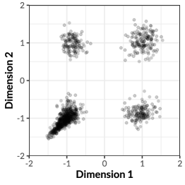
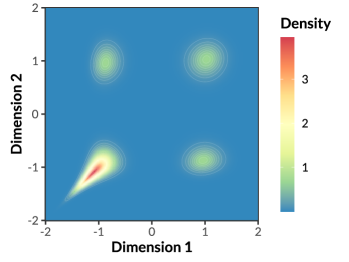
Figure 5: Normal mixture marginals combined with a Clayton copula.

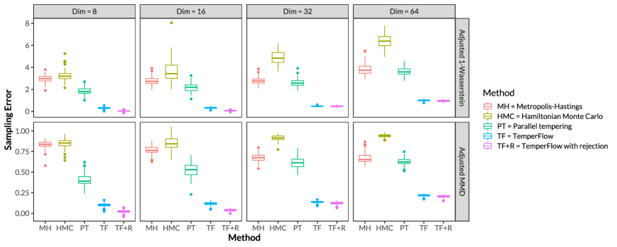
Figure 6: Sampling errors of different methods for the copula-generated distribution.

Under such a design, the target distribution $F(x_{1},\ldots,x_{d})$ has $2^{s}$ modes, which grows exponentially with $s$, and every pair $(X_{i},X_{j})$ is correlated. Therefore, it is a very challenging distribution to sample from even with moderate $s$ and $d$. We first derive the density function $f(x_{1},\ldots,x_{d})$ by computing the partial derivatives of $F$, and then use different methods to sample from $f$ with $s=8$ and $d=8,16,32,64$. That is, each distribution has $256$ modes in total, with varying dimensions.

Similar to the bivariate experiments, we compute the adjusted Wasserstein distances and adjusted MMD between the true and generated samples, and summarize the comparison results in Figure 6 based on 100 repetitions. Figure S5 in the supplementary material also shows the pairwise scatterplots and density contour plots of the generated samples by parallel tempering and TemperFlow, respectively. As expected, TemperFlow samples have desirable quality close to the ground truth, whereas other methods encounter great issues given the huge number of modes and high dimensions.

Of course, both TemperFlow and MCMC are iterative algorithms, so their sampling errors would be affected by the number of iterations, which further impact the overall computing time. We report more comparison results in Section A.3.4 of the supplementary material, and also show the computing time of different algorithms in Table S1. We remark that MCMC only has generation costs, whereas TemperFlow also has a training cost. The main difference is that the generation cost of MCMC is proportional to the number of Markov chain iterations, but for TemperFlow it is nearly fixed and extremely small. Instead, the training cost of TemperFlow scales linearly with the number of optimization iterations.

7 Application: Deep Generative Models

Modern deep learning techniques have attracted enormous attentions from statistical researchers and practitioners, among which deep generative models are a class of important unsupervised learning methods (Salakhutdinov,, 2015; Bond-Taylor et al.,, 2021). Deep generative models attempt to model the statistical distribution of high-dimensional data using DNNs, with wide applications in image synthesis, text generation, etc.

One general class of deep generative models has the form $X=G(Z)$, where $X\in\mathbb{R}^{p}$ is the high-dimensional data point, for example, an image, $Z\in\mathbb{R}^{d}$ is a latent random vector with $d\ll p$, and $G:\mathbb{R}^{d}\rightarrow\mathbb{R}^{p}$ is a DNN, typically called the generator. The distribution of $Z$ is characterized by an energy function $E:\mathbb{R}^{d}\rightarrow\mathbb{R}$, which is also a DNN. In this sense, the pair $(E_{d},G_{d,p})$ defines a deep generative model, where the subscripts $d$ and $p$ indicate the dimensions. There is a great deal of literature discussing the modeling and estimation of $(E_{d},G_{d,p})$; see Che et al., (2020); Pang et al., (2020) for more details. In this section, we treat the functions $E$ and $G$ as known, and focus on the sampling of $p(z)\propto\exp\{-E(z)\}$, as it is the key to generating new data points of $X$.

We first consider generative models for the Fashion-MNIST data set (Xiao et al.,, 2017). The Fashion-MNIST data contain a training set of 60,000 images and a testing set of 10,000 images, each consisting of $28\times 28$ grey-scale pixels. The plot on the left of Figure 7 shows 60 images from the data set. We then build a deep generative model $(E_{2},G_{2,784})$ with $d=2$ based on existing literature (Che et al.,, 2020), and the generated images are shown in the right plot of Figure 7.

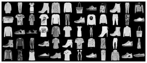
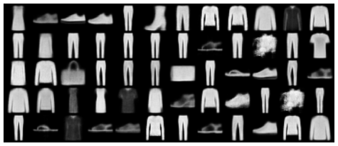
Figure 7: Left: true images from the Fashion-MNIST data set. Right: images generated by a deep generative model with latent dimension $d=2$.

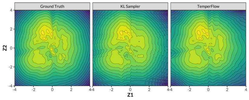
Figure 8: Contour plots of the true log-density function (left), the function learned by the KL sampler (middle), and the function learned by TemperFlow (right).

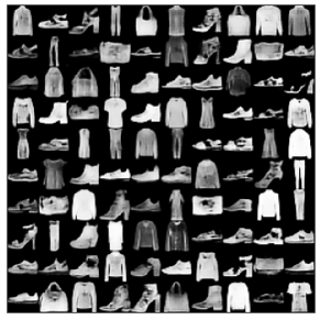
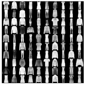
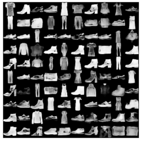
Figure 9: Left: images generated by a deep generative model with latent dimension $d=32$. Middle: images sampled from the model using the KL sampler. Right: images sampled using the TemperFlow sampler.

Since generating images requires independent samples, the measure transport sampling method is especially useful for this task. To this end, we compare the existing KL sampler and our proposed TemperFlow in sampling from $p(z)$. After both samplers are trained, we visualize their estimated log-density functions $\log p(z)$ via contour plots in Figure 8, and also compare them with the ground truth.

It is clear that the true log-density function $\log p(z)$ contains many isolated modes, but the KL sampler only captures a few of them. In contrast, the distribution given by TemperFlow is very close to the ground truth. The difference becomes more evident when the latent dimension $d$ increases. We fit another generative model $(E_{32},G_{32,784})$ with a larger latent dimension $d=32$, and show the generated images in the left plot of Figure 9. Similar to the $d=2$ case, we train both the KL sampler and the TemperFlow sampler from the energy function $E(z)$. In the higher-dimensional case, we are no longer able to visualize the density function directly. Instead, we simulate latent variables $Z_{1},\ldots,Z_{100}\in\mathbb{R}^{32}$ from both samplers, and pass them to the generator $G$ to form images $X_{1}=G(Z_{1}),\ldots,X_{100}=G(Z_{100})\in\mathbb{R}^{784}$. The middle and right plots of Figure 9 show the generated images by KL sampler and TemperFlow, respectively. It is obvious that the KL sampler only generates coat-like and trousers-like images, indicating that it loses a lot of modes of the true distribution. On the other hand, TemperFlow successfully preserves major modes of $p(z)$, further validating the superior performance of the proposed sampler.

Finally, we illustrate a much larger generative model trained from the CelebA data set (Liu et al.,, 2015). Each data point in CelebA is a color human face image of $64\times 64$ size, and we take a subset of the original data set to form the following four categories: females wearing glasses (2677 images), females without glasses (20000 images), males wearing glasses (10346 images), and males without glasses (20000 images). A deep generative model $(E_{100},G_{100,12288})$ is trained on this subset, and Figure 10(a) shows images generated by the model. Naturally, the latent energy function $E$ would reflect these four major modes, and we test the performance of the KL sampler, the MCMC samplers, and TemperFlow by looking at the images generated by them.

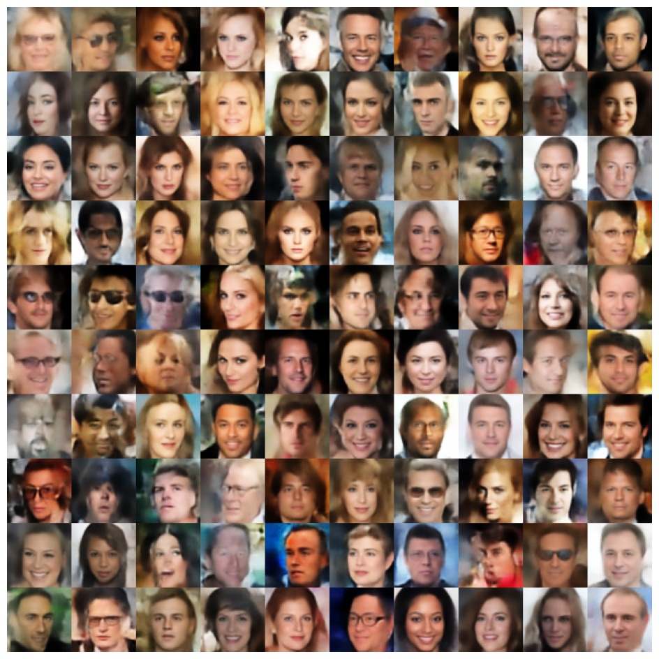
(a) True model sample

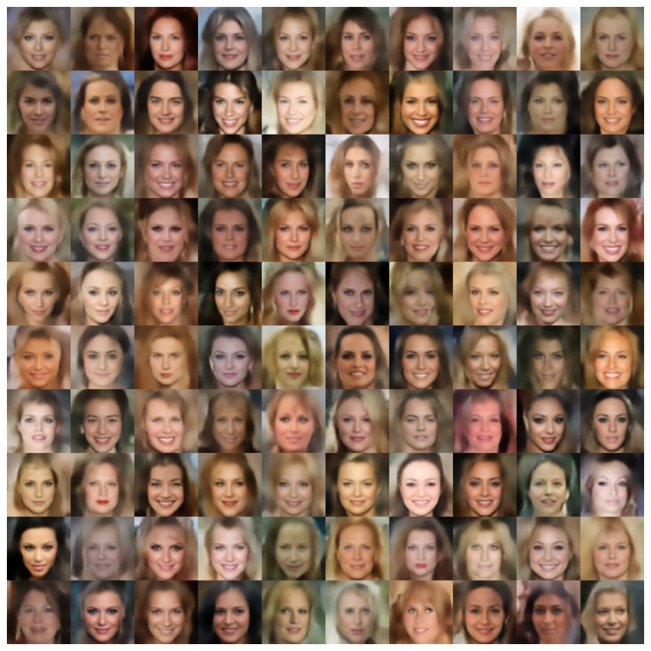
(b) KL sampler

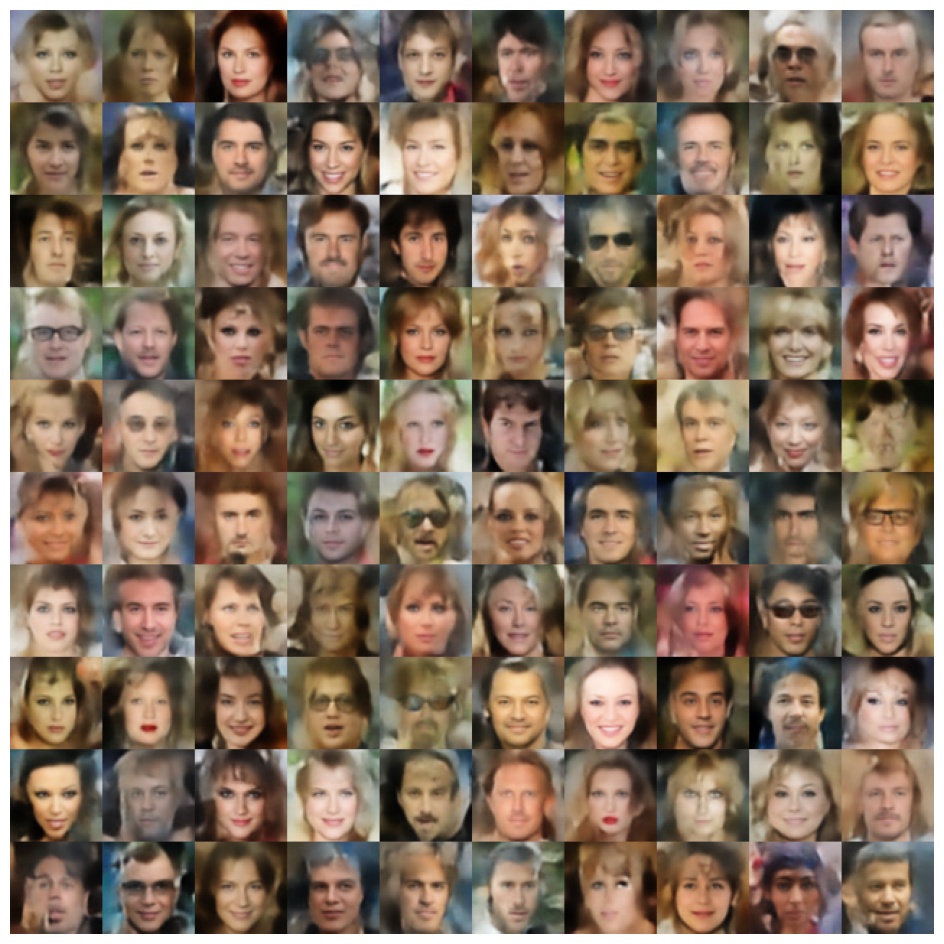
(c) TemperFlow

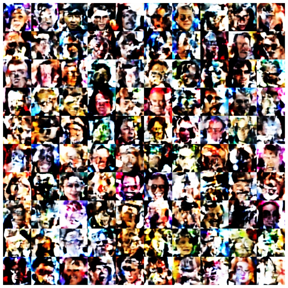
(d) Metropolis–Hastings

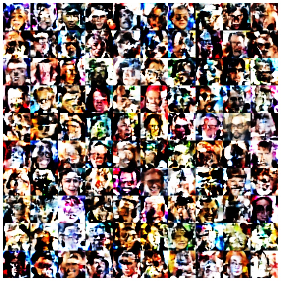
(e) Hamiltonian Monte Carlo

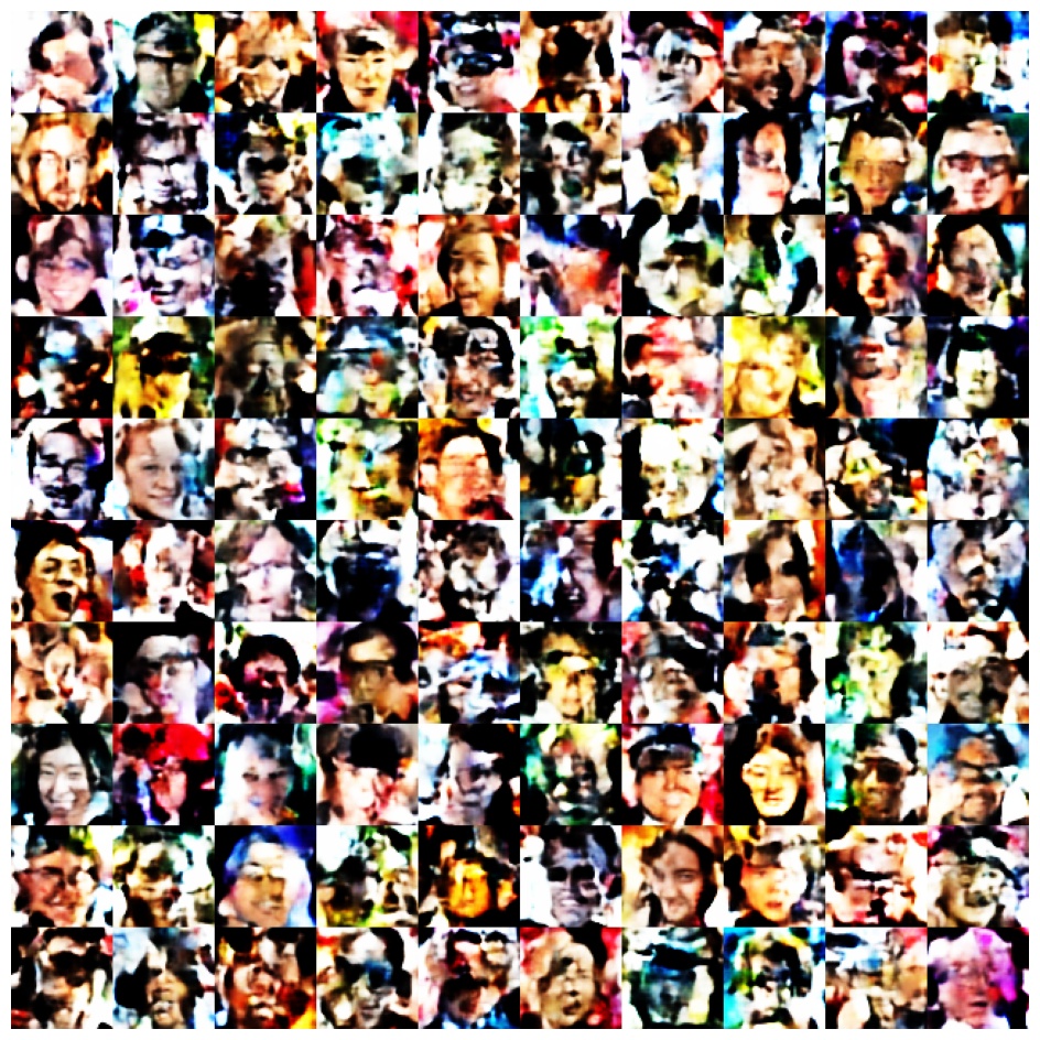
(f) Parallel tempering

Figure 10: (a) Images generated by a deep generative model with latent dimension $d=100$, trained from the CelebA data set. (b)-(f): Images sampled from the model using different samplers.

Figures 10(b)-(f) show the result. Clearly, the KL sampler almost only outputs one class, females without glasses, whereas TemperFlow captures all four classes. On the other hand, MCMC samples hardly generate visible human faces. In summary, all of the examples presented above demonstrate the accuracy and scalability of the TemperFlow sampler.

8 Conclusion and Discussion

In this article, we develop a general-purpose sampler, TemperFlow, to sample from challenging statistical distributions. TemperFlow is inspired by the measure transport framework introduced in Marzouk et al., (2016), but overcomes its critical weaknesses when the target distribution is multimodal. Their fundamental differences are rigorously analyzed using the Wasserstein gradient flow theory, and are also clearly illustrated by various numerical experiments.

One interesting characteristic of TemperFlow is that it transforms the sampling problem into a series of optimization problems, which has the following implications. First, many modern optimization techniques can be exploited directly to accelerate the training of transport maps. Second, it is typically easier to diagnose the convergence of an optimization problem than that of a Markov chain. Third, as we primarily rely on gradient-based optimization methods, the computation of TemperFlow is highly parallelizable, and can greatly benefit from modern computing hardware such as GPUs. All these aspects reflect the huge advantages of TemperFlow in computational efficiency.

As a general-purpose sampling method, TemperFlow can be compared with MCMC on many aspects, but one of the most visible differences is that TemperFlow has a training stage, whereas MCMC directly generates random variates. This difference serves as a guide on which method to use when sampling is needed. Specifically, TemperFlow is especially useful when a large number of independent random variates are requested, and MCMC, on the other hand, may be more suitable in computing expectations for distributions that are continually changing, for example in the Monte Carlo EM algorithm (Wei and Tanner,, 1990; Levine and Casella,, 2001). To this end, we do not position TemperFlow as a substitute for MCMC. Instead, it is viewed as a complement to MCMC and other particle-based methods. We anticipate that these methods can be combined to develop new efficient samplers, which we leave as a future research direction.

Another promising direction is evaluating the goodness-of-fit of models over observed data. Let $X_{1},\ldots,X_{n}\stackrel{{\scriptstyle iid}}{{\sim}}q(x)$ be a random sample from the TemperFlow sampler. Recall that the target density is $p(x)\propto e^{-E(x)}$. We can perform a one-sample goodness-of-fit test $H_{0}:q=p$. The main difficulties are due to complex and high-dimensional models and the unknown normalizing constant for $p(x)$. Traditional goodness-of-fit tests such as the $\chi^{2}$-test and the Kolmogorov–Smirnov test can hardly be applied. The nonparametric one-sample test based on the Stein discrepancy was studied in Chwialkowski et al., (2016). Note that the goodness-of-fit test for the TemperFlow sampler has some special features that are different from the previous problems. In particular, the density $q$ has an explicit formula given the normalizing flow model. This feature allows us to propose a more powerful test, such as the test based on Fisher divergence. The Fisher divergence is stronger than many other divergences, such as total variation, Hellinger distance, and Wasserstein distance (Ley and Swan,, 2013).

Appendix A Appendix

A.1 Invertible Neural Networks

Invertible neural networks (INNs) are a class of neural network models that are invertible with respect to its inputs. An INN can be viewed as a mapping $T:\mathbb{R}^{d}\rightarrow\mathbb{R}^{d}$ such that $T^{-1}$ exists and can be efficiently evaluated, and $T$ is typically a composition of simpler mappings, $T=T_{K}\circ T_{K-1}\circ\cdots\circ T_{1}$, where each $T_{i}$ is invertible. INNs are mainly used to implement normalizing flow models (Tabak and Vanden-Eijnden,, 2010; Tabak and Turner,, 2013; Rezende and Mohamed,, 2015), which can be described as transformations of a probability density through a sequence of invertible mappings.

Normalizing flows were originally developed as nonparametric density estimators (Tabak and Vanden-Eijnden,, 2010; Tabak and Turner,, 2013), and the mappings used there were simple functions with limited expressive powers. After normalizing flows were introduced to the deep learning community, many powerful INN-based models were developed, including affine coupling flows (Dinh et al.,, 2014; Dinh et al.,, 2016), masked autoregressive flows (Papamakarios et al.,, 2017), inverse autoregressive flows (Kingma et al.,, 2016), neural spline flows (Durkan et al.,, 2019), and linear rational spline flows (Dolatabadi et al.,, 2020), among many others. It is worth mentioning that the term “flow” in normalizing flows has a conceptual gap with that in gradient flows, where the latter is the focus of this article. Therefore, to avoid ambiguity, in this article we use invertible neural networks to refer to normalizing flow models, although other forms of normalizing flows also exist, such as the continuous normalizing flows based on ordinary differential equations (Chen et al.,, 2018), and its extension using free-form continuous dynamics (Grathwohl et al.,, 2019).

Take the inverse autoregressive flow as an example. It is the composition of a sequence of invertible mappings, $T=T_{K}\circ T_{K-1}\circ\cdots\circ T_{1}$. For each $i=1,\ldots,K$, let $x=(x_{1},\ldots,x_{d})^{\prime}$ be the input vector, and denote by $y=(y_{1},\ldots,y_{d})^{\prime}=T_{i}(x)$ the output vector. Then $y$ has the following form:

$$y_{1} =\mu_{i1}+\sigma_{i1}x_{1},$$

$$y_{j} =\mu_{ij}(x_{1:j-1})+\sigma_{ij}(x_{1:j-1})x_{j},\quad j=2,\ldots,d,$$

where $x_{1:r}$ means $(x_{1},\ldots,x_{r})^{\prime}$, $\mu_{i1}$, $\sigma_{i1}$ are scalars, and $\mu_{ij},\sigma_{ij}:\mathbb{R}^{j-1}\rightarrow\mathbb{R}$ are neural networks for $j\geq 2$. It can be easily verified that $T_{i}$ is invertible, since

$$x_{1} =(y_{1}-\mu_{i1})/\sigma_{i1},$$

$$x_{2} =(y_{2}-\mu_{i2}(x_{1}))/\sigma_{i2}(x_{1})=(y_{2}-\mu_{i2}((y_{1}-\mu_{i1})/\sigma_{i1}))/\sigma_{i2}((y_{1}-\mu_{i1})/\sigma_{i1}),$$

$$x_{j} =(y_{j}-\mu_{ij}(x_{1:j-1}))/\sigma_{ij}(x_{1:j-1}),\quad j=3,\ldots,d,$$

where each $x_{j}$ is a function of $y_{j}$ and $x_{1:j-1}$, and $x_{1:j-1}$ can be recursively reduced to functions of $y_{1:j-1}$. Furthermore, if the neural networks $\mu_{ij}(\cdot)$ and $\sigma_{ij}(\cdot)$ are differentiable, which can be easily achieved by using smooth activation functions, then each $T_{i}$ and the whole $T$ mapping are also differentiable. In this sense, INNs are diffeomorphisms by design under very mild conditions.

In addition, most INNs have the desirable property that the Jacobian matrix $\nabla T$ is a triangular matrix, so its determinant $\det\nabla T$ is simply the product of diagonal elements. Again using the example above, we can find that

$$\nabla T=\left(\begin{array}[]{cccc}\frac{\partial y_{1}}{\partial x_{1}}&\frac{\partial y_{1}}{\partial x_{2}}&\cdots&\frac{\partial y_{1}}{\partial x_{d}}\\ \frac{\partial y_{2}}{\partial x_{1}}&\frac{\partial y_{2}}{\partial x_{2}}&\cdots&\frac{\partial y_{2}}{\partial x_{d}}\\ \vdots&\vdots&\ddots&\vdots\\ \frac{\partial y_{d}}{\partial x_{1}}&\frac{\partial y_{d}}{\partial x_{2}}&\cdots&\frac{\partial y_{d}}{\partial x_{d}}\end{array}\right)=\left(\begin{array}[]{cccc}\sigma_{i1}&0&\cdots&0\\ &\sigma_{i2}(x_{1})&\cdots&0\\ \vdots&\vdots&\ddots&\vdots\\ &*&\cdots&\sigma_{id}(x_{1:d-1})\end{array}\right),$$

so $\det\nabla T=\sigma_{i1}\cdot\sigma_{i2}(x_{1})\cdots\sigma_{id}(x_{1:d-1})$, and $\det\nabla T>0$ automatically holds if $\sigma_{ij}>0$.

In practice, a permutation operator $P_{\pi}(x_{1},\ldots,x_{d})=(x_{\pi(1)},\ldots,x_{\pi(d)})^{\prime}$ is inserted between each pair of $T_{k}$ and $T_{k-1}$, where $(\pi(1),\ldots,\pi(d))$ is a permutation of $(1,\ldots,d)$. This is because $T_{ij}$ is an affine mapping of $x_{j}$ conditional on $x_{1:j-1}$, and the expressive power of $T$ would be limited if the variables do not change the order.

A.2 Details of Numerical Experiments

A.2.1 Definition of metrics

Given data points $X=(X_{1},\ldots,X_{n})$ and $Y=(Y_{1},\ldots,Y_{m})$, define the discrete 1-Wasserstein distance between $X$ and $Y$ as

$$W(X,Y)=\min_{P\in\Pi}\ \langle P,C\rangle,\quad\Pi=\{P\in\mathbb{R}_{+}^{n\times m}:P\mathbf{1}_{m}=n^{-1}\mathbf{1}_{n},P^{\prime}\mathbf{1}_{n}=m^{-1}\mathbf{1}_{m}\},$$

where $C=(C_{ij})$ is an $n\times m$ matrix with $C_{ij}=\|X_{i}-Y_{j}\|_{1}$. In addition, define the empirical MMD between $X$ and $Y$ as

$$\mathrm{MMD}(X,Y)=\frac{1}{n(n-1)}\sum_{i=1}^{n}\sum_{j\neq i}K(X_{i},X_{j})+\frac{1}{m(m-1)}\sum_{i=1}^{m}\sum_{j\neq i}K(Y_{i},Y_{j})-\frac{2}{nm}\sum_{i=1}^{n}\sum_{j=1}^{m}K(X_{i},Y_{j}),$$

where $K(\cdot,\cdot):\mathbb{R}^{d}\times\mathbb{R}^{d}\rightarrow\mathbb{R}$ is a positive definite kernel function.

Then given the target distribution $p(x)$ and points $X=(X_{1},\ldots,X_{n})$ generated by some sampling algorithm, define the adjusted 1-Wasserstein distance and adjusted MMD between $X$ and $p$ as

$$\tilde{W}(X,p) =W(X,Y)-W(Y,\tilde{Y}),$$

$$\tilde{\mathrm{MMD}}(X,p) =\mathrm{MMD}(X,Y)-\mathrm{MMD}(Y,\tilde{Y}),$$

respectively, where $Y,\tilde{Y}\sim p(x)$ are two independent random samples of size $n$ coming from the true $p(x)$ distribution.

A.2.2 Hyperparameter setting

Gaussian mixture models

For all MCMC samplers, the initial states are generated using standard normal distribution, the first 200 steps are dropped as burn-in, and the subsequent 1000 points are collected as the sample. Metropolis–Hastings uses a normal distribution with standard deviation $\sigma_{\mathrm{MH}}=0.2$ for random walks. Hamiltonian Monte Carlo uses a step size of $\varepsilon=0.2$ and five leapfrog steps in each iteration. The parallel tempering method uses five parallel chains, with inverse temperature parameters equally spaced in the logarithmic scale from 0.1 to 1. At each inverse temperature $\beta$, parallel tempering uses a normal distribution with standard deviation $\text{$\sigma_{\mathrm{PT},\beta}$}=0.2/\sqrt{\beta}$ for random walks.

TemperFlow is initialized by a standard normal distribution and $\beta_{0}=0.1$. The discounting factor for adaptive $\beta$ selection is set to $\alpha=0.5$. For each $\beta_{k}$, the $L^{2}$ sampler is run for 2000 iterations if $\beta_{k}<0.5$, and for 1000 iterations otherwise.

Copula-generated distributions

The hyperparameter setting is similar to that of the Gaussian mixture models, except that $\sigma_{\mathrm{MH}}=\varepsilon=0.1$, $\text{$\sigma_{\mathrm{PT},\beta}$}=0.1/\sqrt{\beta}$, and $\alpha=0.7$.

For the computing time benchmark in Table S1, each MCMC sampler is run for 10200 iterations, with the first 200 steps dropped as burn-in.

A.3 Additional Experiments

A.3.1 KL sampler for normal mixture distributions

In this experiment we extend the example in Section 2.3, and study the impact of the gap between modes on the sampling quality. The first row of Figure S1 is the same as the original example, which applies the KL sampler to the mixture distribution $p_{m}(x)\sim 0.7\cdot N(1,1)+0.3\cdot N(\mu,0.25)$ with $\mu=8$. The second and third rows of Figure S1 reduce the mean gap $\mu$ to 6 and 4, respectively. It can be observed that unless the two modes are sufficiently close to each other, the KL sampler would only capture one mode. This finding also validates the use of tempered distributions in the proposed framework, as tempering has similar effects to make the modes more connected.

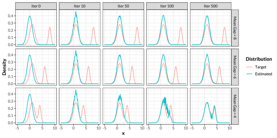
Figure S1: Applying the KL sampler to normal mixture distributions with varying mean gaps. Each column stands for one iteration in the optimization process.

A.3.2 Replacing $L^{2}$ sampler with KL sampler in TemperFlow

In this experiment, we test whether combining the tempering method and KL sampler could achieve the same performance as TemperFlow. This can be viewed as an ablation experiment that replaces the $L^{2}$ sampler with the KL sampler in TemperFlow. We revisit the Gaussian mixture models in Section 6.1, and learn the samplers using TemperFlow and its modified version, respectively. We intentionally let both methods use the same $\beta$-sequence for factor control, and also include the results of the KL sampler without tempering for reference. The results are shown in Figures S2, S3, and S4.

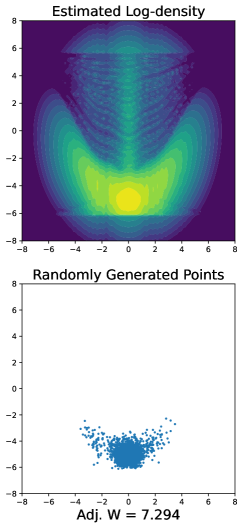
(a)

(b)

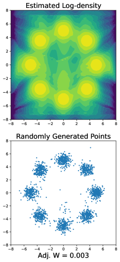
(c)

Figure S2: Sampling from the “Circle” distribution using (a) KL sampler, (b) KL sampler with tempering, and (c) TemperFlow.

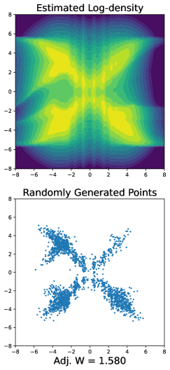
(a)

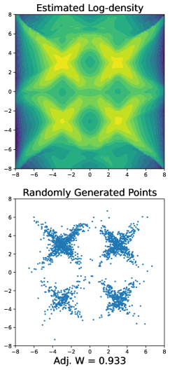
(b)

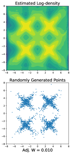
(c)

Figure S3: Sampling from the “Cross” distribution using (a) KL sampler, (b) KL sampler with tempering, and (c) TemperFlow.

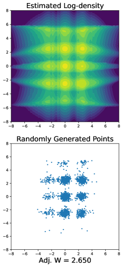
(a)

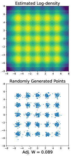
(b)

(c)

Figure S4: Sampling from the “Grid” distribution using (a) KL sampler, (b) KL sampler with tempering, and (c) TemperFlow.

From the plots we can find that, in general, tempering greatly improves the quality of KL samplers. However, even with tempering, KL samplers tend to incorrectly estimate the probability mass of each mode, which is consistent with the finding in Figure 2. This suggests that the $L^{2}$ sampler plays an important role in TemperFlow that cannot be simply replaced by the KL sampler.

A.3.3 Random samples of copula-generated distribution

Figure S5 shows the pairwise scatterplots and density contour plots of the generated samples by parallel tempering and TemperFlow, respectively, for the experiment in Section 6.2 with $s=d=8$.

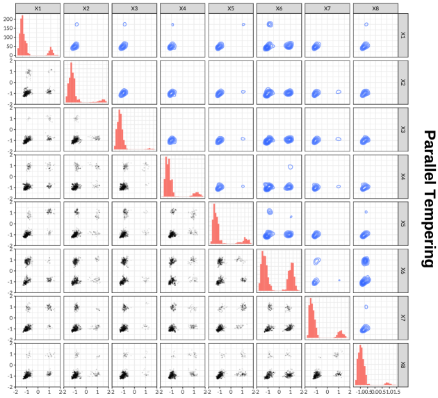
Figure S5: Sampling results of parallel tempering and TemperFlow for the copula-generated distribution with $s=d=8$. The lower triangular part shows pairwise scatterplots of the generated samples, and upper triangular part are the density contour plots. Plots on the diagonal are histograms for the marginal distributions.

A.3.4 Increasing the number of iterations for MCMC samplers

Based on the experiment in Section 6.2, here we increase the number of iterations for MCMC samplers, and again compare their results with TemperFlow. Similar to the previous setting, we drop the first 200 steps as burn-in, but then take one data point every ten iterations. Finally, 1000 data points are collected, so the total number of iterations for MCMC samplers is 10200. Figure S6 demonstrates the sampling errors on this new setting. Compared with Figure 6, we can observe that the overall pattern is very similar, although MCMC is now run with ten times the iterations as before.

Figure S6: Sampling errors of different methods for the copula-generated distribution, with MCMC run for ten times longer than in Figure S6.

A.3.5 Computing time of sampling methods

We report the computing time of different samplers in Table S1 for the distributions in Section 6.2. All samplers are implemented and run on GPUs. As introduced in the article, TemperFlow has a training stage, whose computing time is given in the first row of Table S1. Interestingly, the empirical results show that the training time roughly scales linearly with the dimension of the target distribution. Once the sampler is trained, the generation time of TemperFlow can be virtually ignored, even with a post-processing rejection sampling step. In contrast, MCMC methods have no training costs, but their generation time is proportional to the number of Markov chain iterations. It must also be emphasized that the times for the MCMC methods in Table S1 only reflect the computing cost after a fixed number of iterations, but clearly Figures 6 and S6 suggest that their sampling errors are much higher than those of TemperFlow. Therefore, in practice, a much larger number of iterations is needed for MCMC samplers, which would dramatically increase the total computing time.

Table S1: Computing time for different sampling methods and dimensions. The first row shows the training time of TemperFlow, and the number in the parenthesis is the number of adaptive $\beta$’s used in Algorithm 2. Remaining rows show the time to generate 10,000 points by each algorithm. All timing values are in seconds.

	$p=8$	$p=16$	$p=32$	$p=64$
(TemperFlow Training)	133.7 (17)	309.9 (21)	598.6 (22)	1475.5 (30)
TemperFlow/$10^{4}$	0.00206	0.00449	0.00899	0.0169
TemperFlow+Rej./$10^{4}$	0.0148	0.0263	0.0547	0.0928
MH/$10^{4}$	11.8	16.0	15.8	15.6
HMC/$10^{4}$	80.9	133.0	131.0	130.0
Parallel tempering/$10^{4}$	24.9	32.2	32.5	31.9

A.3.6 Changing the base measure in TemperFlow

When the target distribution $p(x)$ is supported on the whole Euclidean space $\mathbb{R}^{d}$, TemperFlow by default uses the standard multivariate normal as the base measure $\mu_{0}$. If $p(x)$ is known to be supported on a compact set, for example, a hypercube $[-B,B]^{d}$, then $\mu_{0}$ can also be taken as a distribution supported on $[-B,B]^{d}$, such as a uniform distribution. In Figure S7 we show such an example. The target distribution is the same as the “Circle” Gaussian mixture model in Section 6.1, but we restrict its density to the $[-5,5]^{2}$ square. Then we choose the base measure $\mu_{0}$ as the uniform distribution on $[-5,5]^{2}$, and use TemperFlow to estimate the transport map $T$. Figure S7 shows the tempered distribution flow $T_{\sharp}^{(k)}\mu_{0}$ for different inverse temperature parameters $\beta_{k}$. It can be found that TemperFlow again estimates the target distribution well.

Figure S7: Applying TemperFlow to a distribution supported on a closed square. The base measure $\mu_{0}$ is taken to be a uniform distribution.

A.3.7 Comparing different INN architectures

Theoretically, TemperFlow can utilize any variant of INNs to construct $T$, and in practice, we find that spline-based models, such as linear rational splines (Dolatabadi et al.,, 2020), are very powerful, and we use them as the default choice in TemperFlow. To test the performance of different INN architectures, we first consider the two-dimensional distributions studied in Section 6.1, and include three representative INNs for comparison: the inverse autoregressive flows (Kingma et al.,, 2016), the linear rational splines (Dolatabadi et al.,, 2020), and the neural spline flows based on quadratic rational splines (Durkan et al.,, 2019). Figure S8 shows the generated samples using different INN architectures. It is clear that the inverse autoregressive flow is able to capture the outline of the target distribution but is inferior to the other two in the details. Due to this reason, we only study the two spline-based INNs for higher-dimensional problems.

Figure S8: TemperFlow samples based on different INN architectures.

Figure S9 recaps the experiments in Section 6.2, but compares TemperFlow samplers based on linear rational splines and quadratic rational splines, respectively. Table S2 also shows the training and sampling times for each sampler. It can be observed that the two INNs behave similarly, with linear rational splines slightly better than quadratic rational splines in terms of sampling errors, but marginally slower in terms of training time.

Figure S9: Sampling errors of TemperFlow for the copula-generated distribution, based on different INN architectures.

Table S2: Computing time for TemperFlow on the copula-generated distribution, based on two different INN architectures. The interpretation of the numbers is similar to that of Table S1.

		$p=8$	$p=16$	$p=32$	$p=64$
LR	Training	135.6 (17)	320.6 (21)	642.0 (23)	1534.7 (30)
	Sampling/$10^{4}$	0.00215	0.00465	0.00892	0.0173
	Sampling+Rej./$10^{4}$	0.0131	0.0189	0.0401	0.0783
QR	Training	122.9 (17)	284.1 (21)	567.7 (23)	1366.2 (30)
	Sampling/$10^{4}$	0.00156	0.00406	0.00806	0.0156
	Sampling+Rej./$10^{4}$	0.0119	0.0199	0.0358	0.0779

A.3.8 Comparing different discounting factors $\alpha$

In this section we study the impact of the discounting factor $\alpha$ on adaptive temperature selection in TemperFlow. We again consider the copula-generated distribution in Section 6.2, and estimate the transport map using $\alpha=0.5,0.6,0.7,0.8,0.9$. Figure S10 shows the final sampling error of each method, and Table S3 gives the training time and the number of $\beta$’s used. The sampler with $\alpha=0.9$ has abnormal results for dimensions 32 and 64, since we have set the maximum number of $\beta$’s to be 100, and their computations are not finished.

In general, by setting a larger $\alpha$ value, one obtains smaller sampling errors at the expense of more iterations and a longer training time. There is no definite optimal choice for $\alpha$, but Figure S10 suggests that TemperFlow is not very sensitive to the choice of $\alpha$ for $\alpha\geq 0.6$. Furthermore, our empirical results suggest that $\alpha$ can be set small for simple and low-dimensional distributions, whereas it should be larger for more challenging cases.

Figure S10: Sampling errors of TemperFlow for the copula-generated distribution, based on different INN architectures.

Table S3: Training time of TemperFlow on the copula-generated distribution, based on different $\alpha$ values. The number in the parenthesis is the number of adaptive $\beta$’s used in Algorithm 2, and “Max” means TemperFlow has used the maximum number of $\beta$’s, which is set to 100 in the experiments.

	$p=8$	$p=16$	$p=32$	$p=64$
$\alpha=0.5$	86.3 (10)	198.4 (12)	418.4 (14)	938.3 (17)
$\alpha=0.6$	106.1 (13)	236.5 (15)	486.9 (17)	1170.8 (22)
$\alpha=0.7$	135.6 (17)	320.6 (21)	642.0 (23)	1534.7 (30)
$\alpha=0.8$	206.4 (27)	459.7 (32)	984.8 (38)	2404.4 (50)
$\alpha=0.9$	488.6 (73)	1104.2 (87)	2356.0 (Max)	4730.1 (Max)

A.3.9 Variance of the importance sampling estimator

In TemperFlow, we rely on importance sampling to estimate the normalizing constant of the tempered density functions. In general, the variance of importance sampling is largely dependent on the proposal distribution. For example, to estimate the normalizing constant

$$Z_{\beta}=\int\exp\{-\beta E(x)\}\mathrm{d}x=\mathbb{E}_{X\sim h(x)}\exp\{-\beta E(X)-\log h(X)\},$$

the importance sampling estimator $\hat{Z}_{\beta}$ is given by

$$\hat{Z}_{\beta}=\frac{1}{M}\sum_{i=1}^{M}\frac{e^{-\beta E(X_{i})}}{h(X_{i})}\coloneqq\frac{1}{M}\sum_{i=1}^{M}w(X_{i}),\quad X_{i}\sim h(x),$$

where $h(x)$ is the proposal distribution. It can be easily verified that $\mathbb{E}(\hat{Z}_{\beta})=Z_{\beta}$, and

$$\mathrm{Var}(\hat{Z}_{\beta})=\frac{1}{M}\int\frac{[e^{-\beta E(x)}-Z_{\beta}h(x)]^{2}}{h(x)}\mathrm{d}x=\frac{1}{M}\int[w(x)-Z_{\beta}]^{2}h(x)\mathrm{d}x.$$

Clearly, if $h(x)\propto e^{-\beta E(x)}$ , then $\mathrm{Var}(\hat{Z}_{\beta})=0$. In TemperFlow, we use $\hat{r}_{s}(x)\approx Z_{\beta_{s}}^{-1}e^{-\beta_{s}E(x)}$ as the proposal distribution to estimate $Z_{\beta_{s+1}}$, where $\hat{r}_{s}=T_{\sharp}^{(s)}\mu_{0}$ is the estimated tempered distribution. Therefore, as long as $\beta_{s}\approx\beta_{s+1}$, the variance of $\hat{Z}_{\beta_{s+1}}$ would be small.

To verify this claim, we consider the experiment in Section 6.2 with $d=8$, and extract the $\{\hat{r}_{k}\}$ distributions from the training process. We then use the following coefficient of variation to quantify the uncertainty of the importance sampling estimator:

$$\mathrm{CV}(\hat{r}_{k},\beta_{s})=\frac{\sqrt{\widehat{\mathrm{Var}}(\hat{Z}_{\beta_{s}})}}{\hat{Z}_{\beta_{s}}}\quad\text{with }h(x)=\hat{r}_{k}(x),\quad s=0,1,\ldots,K,\ 0\leq k\leq s,$$

where $\widehat{\mathrm{Var}}(\hat{Z}_{\beta})=M^{-1}(M-1)^{-1}\sum_{i=1}^{M}[w(X_{i})-\hat{Z}_{\beta}]^{2}$ is an estimator of $\mathrm{Var}(\hat{Z}_{\beta})$. Intuitively, we expect that $\mathrm{CV}(\hat{r}_{k},\beta_{s})$ is small if $k$ is close to $s$. Figure S11(a) shows the sixteen $\beta$ values selected by TemperFlow, $\beta_{0},\ldots,\beta_{15}$, and Figure S11(b) illustrates the values of $\log(\hat{Z}_{\beta_{s}})$ with $\hat{r}_{k}$ used as the proposal distribution. As expected, each column of the matrix has similar values of $\log(\hat{Z}_{\beta_{s}})$, since the expectation of $\hat{Z}_{\beta_{s}}$ does not depend on the proposal distribution. However, different $\hat{r}_{k}$’s result in different variances of $\hat{Z}_{\beta_{s}}$. Figure S11(c) shows the values of $\log[\mathrm{CV}(\hat{r}_{k},\beta_{s})]$ with different combinations of $(k,s)$, from which we can observe that the diagonal elements, corresponding to $k=s$, has the smallest uncertainty. This is consistent with the theoretical analysis of importance sampling. In TemperFlow, we only have $\hat{r}_{k}$, $k<s$, to estimate $Z_{\beta_{s}}$, so $\hat{r}_{s-1}$ is to some extent the optimal choice for the proposal distribution.

(a)

(b)

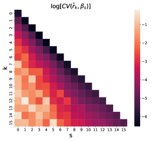
(c)

Figure S11: (a) $\beta$ values selected by TemperFlow. (b) Values of $\log(\hat{Z}_{\beta_{s}})$ with $\hat{r}_{k}$ used as the proposal distribution. (c) Values of $\log[\mathrm{CV}(\hat{r}_{k},\beta_{s})]$ with different $(k,s)$.

A.4 Proof of Proposition 1

By definition, $\mathcal{G}(T)=\mathcal{G}_{1}(T)-\mathcal{G}_{2}(T)$, where $\mathcal{G}_{1}(T)=\int q(x)\log q(x)\mathrm{d}x$ and $\mathcal{G}_{2}(T)=\int q(x)\log p(x)\mathrm{d}x$. Let $\omega=T_{\sharp}\mu_{0}$ and $\nu=A_{\sharp}\omega=(A\circ T)_{\sharp}\mu_{0}$ for some mapping $A:\mathbb{R}^{d}\rightarrow\mathbb{R}^{d}$, and then the density function of $\nu$, denoted by $r$, is given by $r=(q/\det(\nabla A))\circ A^{-1}$. For any function $f:\mathbb{R}\rightarrow\mathbb{R}$, we have

$$\int f(r(x))\mathrm{d}x=\int f\left(\frac{q(A^{-1}(y))}{\det((\nabla A\circ A^{-1})(y))}\right)\mathrm{d}y=\int f\left(\frac{q(x)}{\det(\nabla A(x))}\right)\det(\nabla A(x))\mathrm{d}x.$$

Take $f(x)=x\log(x)$, and then we obtain

$$\mathcal{G}_{1}(A\circ T) =\int r(x)\log r(x)\mathrm{d}x=\int q(x)\left[\log q(x)-\log\det(\nabla A(x))\right]\mathrm{d}x$$

$$=\mathcal{G}_{1}(T)-\int\log\det(\nabla A(x))\mathrm{d}\omega(x).$$

Let $I:\mathbb{R}^{d}\rightarrow\mathbb{R}^{d}$ denote the identity map and $I_{d}$ the $d\times d$ identity matrix. Consider $A=I+\varepsilon\Psi\circ T^{-1}$ for an arbitrary $\Psi\in\mathbb{H}$, and then $\nabla A(x)=I_{d}+\varepsilon G(x)$ with $G=\nabla(\Psi\circ T^{-1})$.

Let $l(\varepsilon;x)=\log\det(I_{p}+\varepsilon G(x))$, and then by Taylor’s theorem,

$$l(\varepsilon;x)=l(0;x)+l^{\prime}(0;x)\varepsilon+\frac{1}{2}\int_{0}^{\varepsilon}l^{\prime\prime}(t;x)(\varepsilon-t)\mathrm{d}t.$$

It can be verified that $l^{\prime}(\varepsilon;x)=\mathrm{tr}\{U(\varepsilon;x)\}$ and $l^{\prime\prime}(\varepsilon;x)=-\mathrm{tr}\{[U(\varepsilon;x)]^{2}\}$, where $U(\varepsilon;x)=[I_{d}+\varepsilon G(x)]^{-1}G(x)$, so

$$\int\log\det(\nabla A(x))\mathrm{d}\omega(x)=\varepsilon\int\mathrm{tr}\{G(x)\}\mathrm{d}\omega(x)-\frac{1}{2}\int\left[\int_{0}^{\varepsilon}\mathrm{tr}\{[U(t;x)]^{2}\}(\varepsilon-t)\mathrm{d}t\right]\mathrm{d}\omega(x).$$

Let $\sigma_{1}(M)\geq\cdots\geq\sigma_{d}(M)$ be the ordered singular values of a matrix $M$, and then by Von Neumann’s trace inequality, we have

$$\left|\mathrm{tr}\{[U(t;x)]^{2}\}\right|\leq\sum_{i=1}^{d}[\sigma_{i}(U(t;x))]^{2}=\sum_{i=1}^{d}[\sigma_{i}(M_{1}^{-1}M_{2})]^{2},$$

where $M_{1}=I_{d}+tG(x)$ and $M_{2}=G(x)$. Moreover, Theorem 3.3.14(b) of Horn and Johnson, (1991) shows that

$$\sum_{i=1}^{d}[\sigma_{i}(M_{1}^{-1}M_{2})]^{2}\leq\sum_{i=1}^{d}[\sigma_{i}(M_{1}^{-1})\sigma_{i}(M_{2})]^{2}=\sum_{i=1}^{d}\left[\frac{\sigma_{i}(M_{2})}{\sigma_{d-i+1}(M_{1})}\right]^{2}.$$

By assumption (a), $\sigma_{i}(M_{2})\leq\sigma_{1}(M_{2})=\|G(x)\|_{\mathrm{op}}\leq C_{\Psi,T}$, and Theorem 3.3.16(c) of Horn and Johnson, (1991) indicates that $\sigma_{i}(M_{1})\geq 1-|t|\sigma_{1}(G(x))\geq 1-|t|C_{\Psi,T}$. Therefore, for all $|t|<1/(2C_{\Psi,T})$, we have $\sigma_{i}(M_{1})\geq 1/2$, and hence

$$\left|\mathrm{tr}\{[U(t;x)]^{2}\}\right|\leq\sum_{i=1}^{d}\left[\frac{\sigma_{i}(M_{2})}{\sigma_{d-i+1}(M_{1})}\right]^{2}\leq 4dC_{\Psi,T}^{2}.$$

As a result, for $0\leq\varepsilon\leq 1/(2C_{\Psi,T})$,

$$\left|\int\left[\int_{0}^{\varepsilon}\mathrm{tr}\{[U(t;x)]^{2}\}(\varepsilon-t)\mathrm{d}t\right]\mathrm{d}\omega(x)\right|\leq 4dC_{\Psi,T}^{2}\int_{0}^{\varepsilon}(\varepsilon-t)\mathrm{d}t=2dC_{\Psi,T}^{2}\varepsilon^{2},$$

and the case of $\varepsilon<0$ can be proved similarly. This implies that

$$\left.\frac{\mathrm{d}}{\mathrm{d}\varepsilon}\int\log\det(\nabla A(x))\mathrm{d}\omega(x)\right|_{\varepsilon=0}=\int\mathrm{tr}\{G(x)\}\mathrm{d}\omega(x),$$

where $\int\mathrm{tr}\{G(x)\}\mathrm{d}\omega(x)$ exists since $|\mathrm{tr}(G(x))|\leq\sum_{i=1}^{d}\sigma_{i}(G(x))\leq dC_{\Psi,T}$. Consequently,

$$\left.\frac{\mathrm{d}}{\mathrm{d}\varepsilon}\mathcal{G}_{1}(T+\varepsilon\Psi)\right|_{\varepsilon=0}=\left.\frac{\mathrm{d}}{\mathrm{d}\varepsilon}\mathcal{G}_{1}(A\circ T)\right|_{\varepsilon=0}=-\int\mathrm{tr}\left\{G(x)\right\}\mathrm{d}\omega(x)=-\int\nabla\cdot(\Psi\circ T^{-1})\mathrm{d}\omega,$$

where $\nabla\cdot F$ is the divergence of a vector field $F$. For a scalar-valued function $\varphi$, the divergence operator satisfies the product rule $\nabla\cdot(\varphi F)=(\nabla\varphi)\cdot F+\varphi(\nabla\cdot F)$, so

$$\int\nabla\cdot(\Psi\circ T^{-1})\mathrm{d}\omega =\int q(x)\left(\nabla\cdot(\Psi\circ T^{-1})\right)(x)\mathrm{d}x$$

$$=\int\nabla\cdot(q(\Psi\circ T^{-1}))\mathrm{d}\lambda-\int\langle\nabla q,\Psi\circ T^{-1}\rangle\mathrm{d}\lambda$$

$$=\int\nabla\cdot(q(\Psi\circ T^{-1}))\mathrm{d}\lambda-\int\langle\nabla\log q,\Psi\circ T^{-1}\rangle\mathrm{d}\omega$$

$$=\int\nabla\cdot(q(\Psi\circ T^{-1}))\mathrm{d}\lambda-\int\langle\nabla\log q\circ T,\Psi\rangle\mathrm{d}\mu_{0}.$$

Under the assumption that $\lim_{\|x\|\rightarrow\infty}\|q(x)\Psi(T^{-1}(x))\|=0$, we have $\int\nabla\cdot(q(\Psi\circ T^{-1}))\mathrm{d}\lambda=0$, so $\delta\mathcal{G}_{1}/\delta T=\nabla\log q\circ T$.

For the second part, we have $\mathcal{G}_{2}(T)=\int\log p(T(x))\mathrm{d}\mu_{0}(x)$ according to the definition of the pushforward operator. By Taylor’s theorem,

$$\log p(T+\varepsilon\Psi)-\log p(T)=\varepsilon\langle\nabla\log p\circ T,\Psi\rangle+\frac{1}{2}\varepsilon^{2}\Psi^{\prime}\left[\nabla^{2}(\log p)\right](T+c\varepsilon\Psi)\Psi$$

for some $c\in(0,1)$. Since we have assumed that $\|\nabla^{2}(\log p)\|_{\mathrm{op}}\leq c$, we get

$$\int\left|\Psi^{\prime}\left[\nabla^{2}(\log p)\right](T+c\varepsilon\Psi)\Psi\right|\mathrm{d}\mu_{0}\leq c\int\|\Psi(x)\|^{2}\mathrm{d}\mu_{0}(x)<\infty,$$

and then

$$\left.\frac{\mathrm{d}}{\mathrm{d}\varepsilon}\mathcal{G}_{2}(T+\varepsilon\Psi)\right|_{\varepsilon=0} =\lim_{\varepsilon\rightarrow 0}\frac{\mathcal{G}_{2}(T+\varepsilon\Psi)-\mathcal{G}_{2}(T)}{\varepsilon}$$

$$=\lim_{\varepsilon\rightarrow 0}\varepsilon^{-1}\int\left[\varepsilon\langle\nabla\log p\circ T,\Psi\rangle+\frac{1}{2}\varepsilon^{2}\Psi^{\prime}\left[\nabla^{2}(\log p)\right](T+c\varepsilon\Psi)\Psi\right]\mathrm{d}\mu_{0}$$

$$=\int\langle\nabla\log p\circ T,\Psi\rangle\mathrm{d}\mu_{0}=\langle\nabla\log p\circ T,\Psi\rangle_{\mathbb{H}}.$$

As a result, $\delta\mathcal{G}_{2}/\delta T=\nabla\log p\circ T$.

Combining the results above, it is easy to find that $\delta\mathcal{G}/\delta T=\delta\mathcal{G}_{1}/\delta T-\delta\mathcal{G}_{2}/\delta T=\nabla(\log q-\log p)\circ T$.

A.5 Proof of Theorem 1

The first part of the theorem is the consequence of several classical and recent results. We first show that if the probability measure $\mu$ has a log-concave density $p(x)$, then it satisfies the Poincaré inequality

$$\int f^{2}\mathrm{d}\mu-\left(\int f\mathrm{d}\mu\right)^{2}\leq C_{P}\int\|\nabla f\|^{2}\mathrm{d}\mu$$ (12)

for all locally Lipschitz $f\in L^{2}(\mu)$, where $C_{P}>0$ is independent of $f$. Indeed, Cheeger, (1970) shows that (12) holds with $C_{P}=4/\psi_{\mu}^{2}$, where

$$\psi_{\mu}=\inf_{S\subset\mathbb{R}^{d}}\frac{\int_{\partial S}p(x)\mathrm{d}x}{\min\left\{\mu(S),\mu(S^{c})\right\}}$$

is called the isoperimetric coefficient of $\mu$. Moreover, Theorem 1 of Chen, (2021) proves that for any integers $d,l\geq 1$,

$$\psi_{\mu}\geq\frac{1}{[c\cdot l(\log(d)+1)]^{l/2}\cdot d^{16/l}\cdot\sqrt{\sigma^{2}}}$$

for some universal constant $c>0$, where $\sigma^{2}$ is the spectral norm of the covariance matrix of $\mu$. For convenience, let $l_{1}\equiv l_{1}(d)=\log(d)+1$, $l_{2}=\log(l_{1})+1$, $L_{1}=\sqrt{l_{1}/l_{2}}$, and $L_{2}=\sqrt{l_{1}l_{2}}$. Take $l=\lceil L_{1}\rceil$, where $\lceil x\rceil$ is the smallest integer greater than or equal to $x$. It is easy to verify that $L_{1}$ is increasing in $d$ and $L_{1}\geq 1$, so we must have $L_{1}\leq l=\lceil L_{1}\rceil\leq 2L_{1}$. Also note that $L_{1}\leq\sqrt{l_{1}}$ and

$$\log(L_{1})\leq\frac{1}{2}\log(l_{1})<\frac{1}{2}l_{2},\qquad L_{1}\log(l_{1})<L_{1}l_{2}=L_{2},\qquad L_{1}\log(L_{1})<L_{1}\cdot\frac{1}{2}l_{2}=\frac{1}{2}L_{2},$$

so

$$\log\left\{[c\cdot l(\log(d)+1)]^{l/2}\cdot d^{16/l}\right\} =\frac{l}{2}\cdot\log(c\cdot l\cdot l_{1})+\frac{16}{l}\log(d)$$

$$\leq L_{1}\left[\log(2c)+\log(L_{1})+\log(l_{1})\right]+\frac{16}{L_{1}}\cdot l_{1}$$

$$\leq\log(2c)L_{1}+\frac{3}{2}L_{2}+16L_{2}.$$

Obviously $L_{1}\leq L_{2}$, so there exists a constant $c^{\prime}>0$ such that $\log\left\{[c\cdot l(\log(d)+1)]^{l/2}\cdot d^{16/l}\right\}\leq c^{\prime}L_{2}$ and

$$\psi_{\mu}\geq\frac{1}{e^{c^{\prime}L_{2}}\cdot\sqrt{\sigma^{2}}}.$$

Combining the results above, we can take $C_{P}=4\sigma^{2}e^{2c^{\prime}L_{2}}$.

Next, Corollary 4 of Chewi et al., (2020) states that if $p(x)$ satisfies the Poincaré inequality (12), then the law $\{\nu_{t}\}$ of the Langevin diffusion

$$\mathrm{d}X_{t}=\nabla_{x}\log p(X_{t})\mathrm{d}t+\sqrt{2}\mathrm{d}B_{t},$$

where $B_{t}$ is the Brownian motion on $\mathbb{R}^{d}$, satisfies $\mathcal{F}(\nu_{t})\leq e^{-2t/C_{P}}\chi^{2}(\nu_{0}\|\mu)$. It is known that the law of the Langevin diffusion is the gradient flow of the KL divergence (Jordan et al.,, 1998), so $\mu_{t}$ and $\nu_{t}$ have the same marginal distributions. Therefore, we also have $\mathcal{F}(\mu_{t})\leq e^{-2t/C_{P}}\chi^{2}(\mu_{0}\|\mu)$. Plugging in the expression of $C_{P}$ and absorbing constants into $c^{\prime}$, we get the stated result.

For the second part, (6) and the equation $\mathbf{v}_{t}(x)=-\nabla\left[\log p_{t}(x)-\log p(x)\right]$ indicate that

$$\frac{\mathrm{d}}{\mathrm{d}t}\mathcal{F}(\mu_{t})=-\int\left\|\nabla\log\frac{\mathrm{d\mu_{t}}}{\mathrm{d}\mu}\right\|^{2}\mathrm{d}\mu_{t}.$$

Let $f=\sqrt{\mathrm{d}\mu_{t}/\mathrm{d}\mu}$, and then

$$\left\|\nabla\log\frac{\mathrm{d\mu_{t}}}{\mathrm{d}\mu}\right\|^{2}=\left\|\nabla\log(f^{2})\right\|^{2}=4\left\|\nabla\log f\right\|^{2}=\frac{4}{f^{2}}\left\|\nabla f\right\|^{2}.$$

Therefore,

$$\frac{\mathrm{d}}{\mathrm{d}t}\mathcal{F}(\mu_{t})=-\frac{4\mathrm{d}\mu}{\mathrm{d}\mu_{t}}\int\|\nabla f\|^{2}\mathrm{d}\mu_{t}=-4\int\|\nabla f\|^{2}\mathrm{d}\mu.$$

By the Poincaré inequality (12), we have

$$\frac{\mathrm{d}}{\mathrm{d}t}\mathcal{F}(\mu_{t}) \leq-\frac{4}{C_{P}}\left[\int f^{2}\mathrm{d}\mu-\left(\int f\mathrm{d}\mu\right)^{2}\right]=-\frac{4}{C_{P}}\left[\int\frac{\mathrm{d}\mu_{t}}{\mathrm{d}\mu}\mathrm{d}\mu-\left(\int\sqrt{\frac{\mathrm{d}\mu_{t}}{\mathrm{d}\mu}}\mathrm{d}\mu\right)^{2}\right].$$

$$=-\frac{4}{C_{P}}\left[1-\left(\int\sqrt{\frac{\mathrm{d}\mu_{t}}{\mathrm{d}\lambda}\cdot\frac{\mathrm{d}\mu}{\mathrm{d}\lambda}}\mathrm{d}\lambda\right)^{2}\right].$$

Note that

$$2H^{2}(\mu,\nu) =\int(\sqrt{\mathrm{d}\mu/\mathrm{d}\lambda}-\sqrt{\mathrm{d}\nu/\mathrm{d}\lambda})^{2}\mathrm{d}\lambda=\int\mathrm{d}\mu+\int\mathrm{d}\nu-2\int\sqrt{\mathrm{d}\mu/\mathrm{d}\lambda}\cdot\sqrt{\mathrm{d}\nu/\mathrm{d}\lambda}\mathrm{d}\lambda$$

$$=2\left[1-\int\sqrt{\mathrm{d}\mu/\mathrm{d}\lambda}\cdot\sqrt{\mathrm{d}\nu/\mathrm{d}\lambda}\mathrm{d}\lambda\right],$$

so

$$\frac{\mathrm{d}}{\mathrm{d}t}\mathcal{F}(\mu_{t})\leq-\frac{4}{C_{P}}\left[1-\left(1-H^{2}(\mu_{t},\mu)\right)^{2}\right]=-\frac{4}{C_{P}}\left[2-H^{2}(\mu_{t},\mu)\right]\cdot H^{2}(\mu_{t},\mu)\leq-\frac{4}{C_{P}}H^{2}(\mu_{t},\mu).$$

The last inequality holds since $0\leq H(\mu,\nu)\leq 1$. Finally, plugging in the expression of $C_{P}$ yields the result.

A.6 Proof of Theorem 2

For the brevity of notation we let $q(x)\equiv p_{t^{*}}(x)$, and $\mathcal{F}$ stands for the $\phi$-divergence-based functional $\mathcal{F}_{\phi}$. By definition,

$$\mathcal{F}(\mu_{t}) =\mathcal{D}_{\phi}(\mu_{t}\|\mu)=\int p(x)\phi\left(\frac{q(x)}{p(x)}\right)\mathrm{d}x$$

$$=\alpha\int h(x)\phi\left(\frac{q(x)}{p(x)}\right)\mathrm{d}x+(1-\alpha)\int h(x-\mu)\phi\left(\frac{q(x)}{p(x)}\right)\mathrm{d}x$$

$$=\alpha\int h(x)\phi\left(\frac{q(x)}{p(x)}\right)\mathrm{d}x+(1-\alpha)\int h(x)\phi\left(\frac{q(x+\mu)}{p(x+\mu)}\right)\mathrm{d}x,$$

$$\frac{q(x)}{p(x)} =\frac{\gamma h(x)+(1-\gamma)h(x-\mu)}{\alpha h(x)+(1-\alpha)h(x-\mu)}=1+\frac{(\gamma-\alpha)(h(x)-h(x-\mu))}{\alpha h(x)+(1-\alpha)h(x-\mu)}.$$

Using the elementary inequality $(a+b)/(c+d)\leq a/c+b/d$ for any $a,b,c,d\geq 0$, we have

$$\frac{p(x)}{q(x)}\leq\frac{\alpha}{\gamma}+\frac{1-\alpha}{1-\gamma}\coloneqq c_{1}^{-1}(\alpha,\gamma),\quad\frac{q(x)}{p(x)}\leq\frac{\gamma}{\alpha}+\frac{1-\gamma}{1-\alpha}\coloneqq c_{2}(\alpha,\gamma).$$

Therefore, $0<c_{1}\leq q(x)/p(x)\leq c_{2}<\infty$ for all $x\in\mathbb{R}^{d}$, and we denote $D_{1}=\max_{x\in[c_{1},c_{2}]}|\phi(x)|$ and $D_{2}=\max_{x\in[c_{1},c_{2}]}|\phi^{\prime\prime}(x)|$. Therefore,

$$\left|\phi\left(\frac{q(x)}{p(x)}\right)\right|\leq D_{1},\quad\left|\phi\left(\frac{q(x+\mu)}{p(x+\mu)}\right)\right|\leq D_{1},\quad\forall x,\mu\in\mathbb{R}^{d}.$$

Moreover, by assumption (a), we have for any fixed $x$, $\lim_{\|\mu\|\rightarrow\infty}\phi(q(x)/p(x))=\phi(\gamma/\alpha)$ and $\lim_{\|\mu\|\rightarrow\infty}\phi(q(x+\mu)/p(x+\mu))=\phi((1-\gamma)/(1-\alpha))$. Since $\int Dh(x)\mathrm{d}x=D<\infty$, by the dominated convergence theorem it holds that

$$\lim_{\|\mu\|\rightarrow\infty}\int h(x)\phi\left(\frac{q(x)}{p(x)}\right)\mathrm{d}x =\int h(x)\phi\left(\frac{\gamma}{\alpha}\right)\mathrm{d}x=\phi\left(\frac{\gamma}{\alpha}\right),$$

$$\lim_{\|\mu\|\rightarrow\infty}\int h(x)\phi\left(\frac{q(x+\mu)}{p(x+\mu)}\right)\mathrm{d}x =\int h(x)\phi\left(\frac{1-\gamma}{1-\alpha}\right)\mathrm{d}x=\phi\left(\frac{1-\gamma}{1-\alpha}\right),$$

which gives the first result.

For the second part, by definition,

$$\nabla\left(\frac{q(x)}{p(x)}\right) =(\alpha-\gamma)\cdot\nabla\left(\frac{h(x-\mu)-h(x)}{p(x)}\right)$$

$$=\frac{\alpha-\gamma}{[p(x)]^{2}}\cdot\left\{p(x)[\nabla h(x-\mu)-\nabla h(x)]-[h(x-\mu)-h(x)]\nabla p(x)\right\}$$

$$=\frac{\alpha-\gamma}{[p(x)]^{2}}\cdot\left[h(x)\nabla h(x-\mu)-h(x-\mu)\nabla h(x)\right]$$

$$=(\alpha-\gamma)\left[\frac{h(x)}{p(x)}\right]^{2}\nabla\left(\frac{h(x-\mu)}{h(x)}\right).$$

Define $\delta(x,\mu)=V(x-\mu)-V(x)$, and then

$$\frac{h(x)}{p(x)}=\frac{h(x)}{\alpha h(x)+(1-\alpha)h(x-\mu)}=\frac{1}{\alpha+(1-\alpha)\exp\{-\delta(x,\mu)\}}.$$

Take $c=\min\{\alpha,1-\alpha\}$ and define $\sigma(x)=1/(1+e^{-x})$, and then $h(x)/p(x)\leq\sigma(\delta(x,\mu))/c$. Moreover, $\nabla(h(x-\mu)/h(x))=\nabla(e^{-\delta(x,\mu)})=-e^{-\delta(x,\mu)}\nabla_{x}\delta(x,\mu)$. By assumption (b), $\|\nabla_{x}\delta(x,\mu)\|=\|\nabla V(x-\mu)-\nabla V(x)\|\leq C_{1}\|\mu\|^{k}$ for sufficiently large $\|\mu\|$, so

$$\left\|\nabla\left(\frac{q(x)}{p(x)}\right)\right\|\leq\frac{|\alpha-\gamma|}{c^{2}}\cdot[\sigma(\delta(x,\mu))]^{2}e^{-\delta(x,\mu)}\cdot C_{1}\|\mu\|^{k}\leq\frac{C_{1}|\alpha-\gamma|}{c^{2}}\cdot\|\mu\|^{k}e^{-|\delta(x,\mu)|},$$ (13)

where the second inequality is due to the fact that $[\sigma(x)]^{2}e^{-x}\leq e^{-|x|}$.

Next, Lemma 2.1 of Gao et al., (2019) shows that $(\delta\mathcal{F}/\delta\nu)(\rho)=\phi^{\prime}(\mathrm{d}\rho/\mathrm{d}\mu)$, and hence $\mathbf{v}_{t}(x)=-\phi^{\prime\prime}(p_{t}(x)/p(x))\nabla[p_{t}(x)/p(x)]$. Plugging in (13), we have

$$\|\mathbf{v}_{t^{*}}(x)\|\leq\frac{C_{1}D_{2}|\alpha-\gamma|}{c^{2}}\cdot\|\mu\|^{k}e^{-|\delta(x,\mu)|}.$$

Therefore,

$$0\leq-\left.\frac{\mathrm{d}\mathcal{F}(\mu_{t})}{\mathrm{d}t}\right|_{t=t^{*}}=\int q(x)\|\mathbf{v}_{t^{*}}(x)\|^{2}\mathrm{d}x\leq\frac{C_{1}D_{2}|\alpha-\gamma|}{c^{2}}\cdot\|\mu\|^{k}\int q(x)e^{-|\delta(x,\mu)|}\mathrm{d}x.$$

By definition,

$$\int q(x)e^{-|\delta(x,\mu)|}\mathrm{d}x =\gamma\int h(x)e^{-|\delta(x,\mu)|}\mathrm{d}x+(1-\gamma)\int h(x-\mu)e^{-|\delta(x,\mu)|}\mathrm{d}x$$

$$=\gamma\int h(x)e^{-|\delta(x,\mu)|}\mathrm{d}x+(1-\gamma)\int h(x)e^{-|\delta(x+\mu,\mu)|}\mathrm{d}x$$

$$=\gamma\mathbb{E}e^{-|Y_{\mu,1}|}+(1-\gamma)\mathbb{E}e^{-|Y_{\mu,2}|}.$$

Let $g_{1}(y)$ be the density function of $|Y_{\mu,1}|$, and then

$$\mathbb{E}e^{-|Y_{\mu,1}|} =\int_{0}^{C_{2}\|\mu\|}g_{1}(y)e^{-y}\mathrm{d}x+\int_{C_{2}\|\mu\|}^{+\infty}g_{1}(y)e^{-y}\mathrm{d}x$$

$$\leq\int_{0}^{C_{2}\|\mu\|}g_{1}(y)\mathrm{d}x+\int_{C_{2}\|\mu\|}^{+\infty}g_{1}(y)e^{-C_{2}\|\mu\|}\mathrm{d}x$$

$$=P(|Y_{\mu,1}|\leq C_{2}\|\mu\|)+e^{-C_{2}\|\mu\|}P(|Y_{\mu,1}|>C_{2}\|\mu\|)$$

$$\leq P(|Y_{\mu,1}|\leq C_{2}\|\mu\|)+e^{-C_{2}\|\mu\|}.$$

Similarly, we can verify that $\mathbb{E}e^{-|Y_{\mu,2}|}\leq P(|Y_{\mu,2}|\leq C_{2}\|\mu\|)+e^{-C_{2}\|\mu\|}$. Finally, by assumption (c), we obtain

$$C_{1}\|\mu\|^{k}\int q(x)e^{-|\delta(x,\mu)|}\mathrm{d}x \leq C_{1}\|\mu\|^{k}e^{-C_{2}\|\mu\|}+\gamma C_{1}\|\mu\|^{k}P(|Y_{\mu,1}|\leq C_{2}\|\mu\|)+$$

$$\qquad(1-\gamma)C_{1}\|\mu\|^{k}P(|Y_{\mu,2}|\leq C_{2}\|\mu\|)\rightarrow 0$$

as $\|\mu\|\rightarrow\infty$, which gives the requested conclusion.

A.7 Proof of Theorem 3 and (10)

Let $q_{\beta}(x)=e^{-\beta E(x)}/Z(\beta)$, where $Z(\beta)=\int e^{-\beta E(x)}\mathrm{d}x$. Define the function $\ell(\beta)=\mathrm{KL}(q_{\beta}\|p)$, and we are going to show that $\ell(\beta)$ is decreasing in $\beta$. By definition,

$$\ell(\beta)=\int q_{\beta}(x)\log\frac{q_{\beta}(x)}{p(x)}\mathrm{d}x=\int q_{\beta}(x)[\log q_{\beta}(x)-\log p(x)]\mathrm{d}x.$$

For simplicity let $\zeta(\beta)=\log Z(\beta)$, and then $\log q_{\beta}(x)=-\beta E(x)-\zeta(\beta)$ and $\log p(x)=-E(x)-\zeta(1)$. Therefore,

$$\ell(\beta) =\int q_{\beta}(x)[E(x)+\zeta(1)-\beta E(x)-\zeta(\beta)]\mathrm{d}x$$

$$=(1-\beta)\int q_{\beta}(x)E(x)\mathrm{d}x+\zeta(1)-\zeta(\beta),$$

and

$$\ell^{\prime}(\beta)=-\int q_{\beta}(x)E(x)\mathrm{d}x+(1-\beta)\int\frac{\partial q_{\beta}(x)}{\partial\beta}E(x)\mathrm{d}x-\zeta^{\prime}(\beta).$$

Note that

$$\zeta^{\prime}(\beta) =\frac{Z^{\prime}(\beta)}{Z(\beta)}=\frac{1}{Z(\beta)}\int e^{-\beta E(x)}[-E(x)]\mathrm{d}x=-\int q_{\beta}(x)E(x)\mathrm{d}x,$$

so $\ell^{\prime}(\beta)=(1-\beta)\int[\partial q_{\beta}(x)/\partial\beta]E(x)\mathrm{d}x$. Moreover, since $\partial\log q_{\beta}(x)/\partial\beta=-E(x)-\zeta^{\prime}(\beta)$, we have

$$\frac{\partial q_{\beta}(x)}{\partial\beta}=q_{\beta}(x)\cdot\frac{\partial\log q_{\beta}(x)}{\partial\beta}=-q_{\beta}(x)[E(x)+\zeta^{\prime}(\beta)].$$

Consequently,

$$\ell^{\prime}(\beta) =-(1-\beta)\int q_{\beta}(x)[E(x)+\zeta^{\prime}(\beta)]E(x)\mathrm{d}x$$

$$=-(1-\beta)\left\{\int q_{\beta}(x)E^{2}(x)\mathrm{d}x-\left[\int q_{\beta}(x)E(x)\mathrm{d}x\right]^{2}\right\}.$$ (14)

By Jensen’s inequality, $\int q_{\beta}(x)E^{2}(x)\mathrm{d}x\geq\left[\int q_{\beta}(x)E(x)\mathrm{d}x\right]^{2}$, and the equal sign holds if and only if $E(x)$ is a constant. Since the energy function cannot be a constant over $\mathbb{R}^{d}$, the inequality is strict. As a result, $\ell^{\prime}(\beta)<0$ when $0<\beta<1$, and $\ell^{\prime}(\beta)=0$ only when $\beta=1$. Since $\beta_{t}$ is increasing in $t$, it follows that $\mathcal{F}(\rho_{t})=\ell(\beta_{t})$ is decreasing in $t$.

Finally, (10) can be proved by noting that $\mathrm{d}[\log\ell(e^{\gamma})]/\mathrm{d}\gamma=\beta\cdot\ell^{\prime}(\beta)/\ell(\beta)$, where $\ell^{\prime}(\beta)$ is given in (14), and we show the expression of $\ell(\beta)$ below. By definition,

$$\ell(\beta)=\int q_{\beta}(x)[\log q_{\beta}(x)-\log p(x)]\mathrm{d}x=\int q_{\beta}(x)[\log q_{\beta}(x)+E(x)+\zeta(1)]\mathrm{d}x,$$

where

$$\zeta(1)=\log Z(1)=\log\int\exp\{-E(x)\}\mathrm{d}x=\log\int q_{\beta}(x)\exp\{-E(x)-\log q_{\beta}(x)\}\mathrm{d}x,$$

and then the equation holds.

A.8 Proof of Proposition 2

Since $f(x_{\varepsilon})=\varepsilon^{1/4}$ and $f(x)$ is decreasing for $x\geq 0$, we have $\inf_{Q^{\varepsilon}}f\leq\varepsilon^{1/4}$. Moreover, $\int_{Q^{\varepsilon}}f\mathrm{d}\lambda=2\Phi(x_{\varepsilon}+M\varepsilon^{1/12})-1$, where $\Phi(\cdot)$ is the c.d.f. of the standard normal distribution. For sufficiently small $\varepsilon$, $x_{\varepsilon}=\sqrt{-(\log\varepsilon)/2-\log(2\pi)}>\sqrt{\log(1/\varepsilon)/3}>2$. Then by the well-known inequality $1-\Phi(x)<f(x)/x$ for $x>0$, we have

$$\int_{Q^{\varepsilon}}f\mathrm{d}\lambda>2\Phi(x_{\varepsilon})-1>1-2f(x_{\varepsilon})/x_{\varepsilon}=1-2\varepsilon^{1/4}/x_{\varepsilon}>1-\varepsilon^{1/4}$$

if $\varepsilon$ is small enough. Hence Assumption 1(a) holds.

For convenience let $\delta=M\varepsilon^{1/12}$. Since $f^{-2}(x)=2\pi e^{x^{2}}$ is symmetric about zero and is increasing for $x>0$, the supremum in Assumption 1(b) is achieved when $Q=Q^{\varepsilon}$. It is known that $h(x)=e^{-x^{2}}\int_{0}^{x}e^{y^{2}}\mathrm{d}y<0.6$, so

$$\int_{Q^{\varepsilon}}f^{-2}(x)\mathrm{d}x=4\pi\int_{0}^{x_{\varepsilon}+\delta}e^{x^{2}}\mathrm{d}x=4\pi e^{(x_{\varepsilon}+\delta)^{2}}h(x_{\varepsilon}+\delta)<2.4\pi e^{(x_{\varepsilon}+\delta)^{2}}.$$

Let $l(x)=e^{x^{2}/2}$, and then $l^{\prime}(x)=xl(x)$ and $l^{\prime\prime}(x)=l(x)(x^{2}+1)$, so

$$e^{(x_{\varepsilon}+\delta)^{2}/2}=e^{x_{\varepsilon}^{2}/2}\left[1+x_{\varepsilon}\delta+(1+x_{\varepsilon}^{2})\delta^{2}+O((x_{\varepsilon}\delta)^{3})\right]<Ce^{x_{\varepsilon}^{2}/2}=C\varepsilon^{-1/4}$$

for some constant $C>0$. As a result,

$$\sup_{\begin{subarray}{c}Q\subset Q^{\varepsilon}\\ Q\in\mathcal{Q}\end{subarray}}|Q|^{2/d}\left[\frac{1}{|Q|}\int_{Q}f^{-2}\mathrm{d}\lambda\right]^{1/2}=|Q^{\varepsilon}|^{3/2}\left[\int_{Q^{\varepsilon}}f^{-2}(x)\mathrm{d}x\right]^{1/2}<\sqrt{2.4\pi}C\varepsilon^{-1/4}|Q^{\varepsilon}|^{3/2}.$$

$|Q^{\varepsilon}|$ is at the order of $\sqrt{\log(1/\varepsilon)}$, so Assumption 1(b) holds with $c=3/4$.

Finally, note that

$$\int_{Q^{\varepsilon}}\left[\varepsilon^{1/4}-f(x)\right]_{+}^{2}\mathrm{d}x=2\int_{x_{\varepsilon}}^{x_{\varepsilon}+\delta}\left[\varepsilon^{1/4}-f(x)\right]^{2}\mathrm{d}x.$$

Let $g(x)=\left[\varepsilon^{1/4}-f(x)\right]^{2}$, and then we have $g^{\prime}(x)=-2\left[\varepsilon^{1/4}-f(x)\right]f^{\prime}(x)$ and $g^{\prime\prime}(x)=2[f^{\prime}(x)]^{2}-2\left[\varepsilon^{1/4}-f(x)\right]f^{\prime\prime}(x)$. Since $g(x_{\varepsilon})=g^{\prime}(x_{\varepsilon})=0$ and

$$g^{\prime\prime}(x_{\varepsilon})=2[f^{\prime}(x_{\varepsilon})]^{2}=2x_{\varepsilon}^{2}[f(x_{\varepsilon})]^{2}=2x_{\varepsilon}^{2}\varepsilon^{1/2},$$

by the Taylor expansion we have

$$\frac{1}{2}\int_{Q^{\varepsilon}}\left[\varepsilon^{1/4}-f(x)\right]_{+}^{2}\mathrm{d}x =g(x_{\varepsilon})\delta+\frac{1}{2}g^{\prime}(x_{\varepsilon})\delta^{2}+\frac{1}{6}g^{\prime\prime}(x_{\varepsilon})\delta^{3}+O(\delta^{4})$$

$$=\frac{1}{3}x_{\varepsilon}^{2}\varepsilon^{1/2}\delta^{3}>\frac{M^{3}}{9}\varepsilon^{3/4}\log(1/\varepsilon)>\frac{M^{3}}{9}\varepsilon^{3/4}[\log(1/\varepsilon)]^{3/4}$$

for sufficiently small $\varepsilon$, which verifies Assumption 1(c).

A.9 Technical Lemmas

Let $\lambda$ denote the Lebesgue measure on $\mathbb{R}^{d}$. A function $w$ is called a weight if it is nonnegative and locally integrable on $\mathbb{R}^{d}$. A weight $w$ induces a measure, defined by $w(A)=\int_{A}w\mathrm{d}\lambda$. Denote by $\mathcal{Q}$ the set of balls in $\mathbb{R}^{d}$. A weight $w$ is doubling if $w(2Q)\leq Cw(Q)$ for every $Q\in\mathcal{Q}$, where $2Q$ denotes the ball with the same center as $Q$ and twice its radius, and $C$ is called the doubling constant for $w$. For a measurable set $A\subset\mathbb{R}^{d}$, let $|A|=\lambda(A)$, and we use $\|f\|_{L_{w}^{p}(A)}$ to denote the $w$-weighted $L^{p}$ norm of a vector-valued function $f:\mathbb{R}^{d}\rightarrow\mathbb{R}^{d^{\prime}}$ on $A$, i.e.,

$$\|f\|_{L_{w}^{p}(A)}=\left[\int_{A}\|f(x)\|^{p}w(x)\mathrm{d}x\right]^{1/p},$$

where $\|\cdot\|$ is the Euclidean norm.

Lemma 1 (Theorem 2.14, Chua,, 1993).

Let $1<p\leq q<\infty$ and let $\sigma=v^{-1/(p-1)}$ where $v$ is a weight. Suppose $w$ is a doubling weight. Then for all $Q_{0}\in\mathcal{Q}$ and Lipschitz continuous function $f$ on $Q_{0}$,

$$\|f-f_{Q_{0},w}\|_{L_{w}^{q}(Q_{0})}\leq A(v,w,Q_{0})\|\nabla f\|_{L_{v}^{p}(Q_{0})}$$

where

$$A(v,w,Q_{0})=C(p,q,C_{0})\sup_{\begin{subarray}{c}Q\subset Q_{0}\\ Q\in\mathcal{Q}\end{subarray}}|Q|^{1/d-1}w(Q)^{1/q}\sigma(Q)^{1/p^{\prime}}$$

when $p<q$, and

$$A(v,w,Q_{0})=C(p,r,C_{0})\sup_{\begin{subarray}{c}Q\subset Q_{0}\\ Q\in\mathcal{Q}\end{subarray}}|Q|^{1/d}\left[\frac{1}{|Q|}\int_{Q}w^{r}\mathrm{d}\lambda\right]^{1/(pr)}\left[\frac{1}{|Q|}\int_{Q}\sigma^{r}\mathrm{d}\lambda\right]^{1/(p^{\prime}r)}$$

when $p=q$ for any $r>1$. $C_{0}$ is the doubling constant for $w$, $p^{\prime}=p/(p-1)$, and $f_{Q_{0},w}=w(Q_{0})^{-1}\int_{Q_{0}}fw\mathrm{d}\lambda$.

Lemma 2.

Let $g(x)$ be a density function defined on $\mathbb{R}^{d}$. Then for any ball $Q_{0}\in\mathcal{Q}$ and any Lipschitz continuous function $h$ on $Q_{0}$, the following inequality holds,

$$\int_{Q_{0}}\left|h(x)-h_{Q_{0}}\right|^{2}\mathrm{d}x\leq A(g,d,Q_{0})\int_{Q_{0}}\|\nabla h(x)\|^{2}g(x)\mathrm{d}x,$$

where

$$h_{Q_{0}}=\frac{1}{|Q_{0}|}\int_{Q_{0}}h\mathrm{d}\lambda,\quad A(g,d,Q_{0})=C(d)\sup_{\begin{subarray}{c}Q\subset Q_{0}\\ Q\in\mathcal{Q}\end{subarray}}|Q|^{2/d}\left[\frac{1}{|Q|}\int_{Q}g^{-2}\mathrm{d}\lambda\right]^{1/2},$$

and $C(d)$ is a constant independent of $g$, $h$, and $Q_{0}$.

Proof.

It is easy to verify that $w\equiv 1$ is a doubling weight with doubling constant $C_{0}=2^{d}$. Then take $v=g$, $w=1$, $p=q=r=2$ in Lemma 1, and the conclusion holds. ∎

Lemma 3.

Let $f(x)$ be a continuous function defined on a compact set $S\subset\mathbb{R}^{d}$. Assume $\inf_{S}f(x)<c$ for some constant $c>0$, and denote $M=\int_{S}\left[c-f(x)\right]_{+}^{2}\mathrm{d}x$, where $g_{+}=\max(0,g)$ stands for the positive part of a function $g$. Then for any continuous function $e(x)$ satisfying $\int_{S}[e(x)]^{2}\mathrm{d}x\leq M$, we have $\inf_{S}\ [f(x)+e(x)]\leq c$.

Proof.

Since any $e(x)$ can be replaced by $|e(x)|$ to achieve a larger $\inf_{S}\ [f(x)+e(x)]$ under the same condition $\int_{S}[e(x)]^{2}\mathrm{d}x\leq M$, we can assume that $e(x)\geq 0$ without loss of generality.

Let $h_{c}(x)=\max(c,f(x))$, $e^{*}(x)=h_{c}(x)-f(x)=[c-f(x)]_{+}$, and $u^{*}(x)=[e^{*}(x)]^{2}$. Then it is easy to see that $h_{c}(x)=c$ on $T\coloneqq\{x:f(x)\leq c\}$ and $e^{*}(x)=u^{*}(x)=0$ on $S\backslash T$, implying $M=\int_{S}u^{*}(x)\mathrm{d}x=\int_{T}u^{*}(x)\mathrm{d}x$. For any continuous $u(x)\geq 0$ such that $\int_{S}u(x)\mathrm{d}x\leq M$, we claim that there must exist some point $x_{0}\in T$ such that $u(x_{0})\leq u^{*}(x_{0})$. If this is not true, then

$$\int_{S}u(x)\mathrm{d}x>\int_{T}u^{*}(x)\mathrm{d}x+\int_{S\backslash T}u(x)\mathrm{d}x\geq\int_{T}u^{*}(x)\mathrm{d}x+\int_{S\backslash T}u^{*}(x)\mathrm{d}x=\int_{S}u^{*}(x)\mathrm{d}x=M,$$

which causes a contradiction.

Let $e(x)=\sqrt{u(x)}$, and then it is also true that $e(x_{0})\leq e^{*}(x_{0})$ for some $x_{0}\in T$, implying

$$\inf_{S}\ [f(x)+e(x)]\leq f(x_{0})+e(x_{0})\leq f(x_{0})+e^{*}(x_{0})=h_{c}(x_{0})=c.$$

∎

A.10 Proof of Theorem 4

It is easy to show that the first variation of $\mathcal{L}$ at $g$ is $(\delta\mathcal{L}/\delta g)(g)=2(g-f)$, and then the vector field $\mathbf{v}_{t}$ for the continuity equation $\partial g_{t}/\partial t+\nabla\cdot(\mathbf{v}_{t}g_{t})=0$ is given by $\mathbf{v}_{t}=2\nabla(f-g_{t})$. Let $h_{t}=g_{t}-f$, and then

$$\frac{\mathrm{d}\mathcal{L}(g_{t})}{\mathrm{d}t}=-\int\|2\nabla h_{t}\|^{2}g_{t}\mathrm{d}\lambda=-4\int\|\nabla h_{t}\|^{2}g_{t}\mathrm{d}\lambda.$$

In what follows, we omit the subscript $t$ in $g_{t}$ and $h_{t}$ and the superscript $\varepsilon$ in $Q_{i}^{\varepsilon}$ whenever no confusion is caused. Since $|\mathrm{d}\mathcal{F}(g_{t})/\mathrm{d}t|\leq\varepsilon$, we have $\int\|\nabla h\|^{2}g\mathrm{d}\lambda\leq\varepsilon/4$, and hence

$$\max_{1\leq i\leq K}\int_{Q_{i}}\|\nabla h\|^{2}g\mathrm{d}\lambda\leq\varepsilon/4.$$

By Lemma 2, we have

$$\int_{Q_{i}}\left|h(x)-h_{Q_{i}}\right|^{2}\mathrm{d}x\leq A(g,d,Q_{i})\varepsilon/4,$$ (15)

where

$$A(g,d,Q_{i})=C(d)\sup_{\begin{subarray}{c}Q\subset Q_{i}\\ Q\in\mathcal{Q}\end{subarray}}|Q|^{2/d}\left[\frac{1}{|Q|}\int_{Q}g^{-2}\mathrm{d}\lambda\right]^{1/2}.$$

By Assumptions 1(b) and 2, we have

$$A(g,d,Q_{i})\leq\alpha^{-1}C(d)\sup_{\begin{subarray}{c}Q\subset Q_{i}\\ Q\in\mathcal{Q}\end{subarray}}|Q|^{2/d}\left[\frac{1}{|Q|}\int_{Q}f^{-2}\mathrm{d}\lambda\right]^{1/2}\leq\alpha^{-1}C(d)M_{1}\varepsilon^{-1/4}[\log(1/\varepsilon)]^{c}.$$

Since $M_{2}>0$ in Assumptions 1(c) is a sufficiently large constant, we can take $M_{2}=(4\alpha)^{-1}C(d)M_{1}$, and then (15) leads to

$$\int_{Q_{i}}\left|h(x)-h_{Q_{i}}\right|^{2}\mathrm{d}x\leq M_{2}\varepsilon^{3/4}[\log(1/\varepsilon)]^{c}.$$ (16)

Let $e_{i}(x)=h(x)-h_{Q_{i}}$, and then by definition, $\int_{Q_{i}}e_{i}\mathrm{d}\lambda=0$ and $\int_{Q_{i}}e_{i}^{2}\mathrm{d}\lambda\leq M_{2}\varepsilon^{3/4}[\log(1/\varepsilon)]^{c}$. In Lemma 3, take $S=Q_{i}$, $e=e_{i}$, $M=M_{2}\varepsilon^{3/4}[\log(1/\varepsilon)]^{c}$, and $c=\varepsilon^{1/4}$, and then by Assumption 1(a) we obtain $\inf_{Q_{i}}\ (f+e_{i})\leq\varepsilon^{1/4}$. Since $f+e_{i}$ is continuous and $Q_{i}$ is compact, there must exist a point $x^{*}\in Q_{i}$ such that

$$f(x^{*})+e_{i}(x^{*})=\inf_{Q_{i}}\ (f+e_{i})\leq\varepsilon^{1/4}.$$

Then we obtain

$$h_{Q_{i}}=h(x^{*})-e_{i}(x^{*})=g(x^{*})-f(x^{*})-e_{i}(x^{*})\geq-[f(x^{*})+e_{i}(x^{*})]\geq-\varepsilon^{1/4}.$$ (17)

On the other hand, $\int_{Q}g\mathrm{d}\lambda\leq 1$ and $\int_{Q}f\mathrm{d}\lambda\geq 1-\varepsilon^{1/4}$ by Assumption 1(a), so

$$\varepsilon^{1/4}\geq\int_{Q}(g-f)\mathrm{d}\lambda=\sum_{i=1}^{K}\int_{Q_{i}}(g-f)\mathrm{d}\lambda=\sum_{i=1}^{K}\int_{Q_{i}}(e_{i}+h_{Q_{i}})\mathrm{d}\lambda.$$

Note that $\int_{Q_{i}}e_{i}\mathrm{d}\lambda=0$ and $\int_{Q_{i}}h_{Q_{i}}\mathrm{d}\lambda=h_{Q_{i}}|Q_{i}|$, so we have

$$h_{Q_{i}}|Q_{i}|\leq\sum_{i=1}^{K}h_{Q_{i}}|Q_{i}|\leq\varepsilon^{1/4}.$$ (18)

Combining (17) and (18), and then we get $|h_{Q_{i}}|\leq\max(1,|Q_{i}|^{-1})\cdot\varepsilon^{1/4}.$

Finally, (16) indicates that $\|h-h_{Q_{i}}\|_{L^{2}(Q_{i})}\leq M_{2}^{1/2}\varepsilon^{3/8}[\log(1/\varepsilon)]^{c/2}$, so

$$\|h\|_{L^{2}(Q_{i})} \leq\|h-h_{Q_{i}}\|_{L^{2}(Q_{i})}+\|h_{Q_{i}}\|_{L^{2}(Q_{i})}\leq M_{2}^{1/2}\varepsilon^{3/8}[\log(1/\varepsilon)]^{c/2}+h_{Q_{i}}|Q_{i}|^{1/2}$$

$$\leq M_{2}^{1/2}\varepsilon^{3/8}[\log(1/\varepsilon)]^{c/2}+\max(|Q_{i}|^{1/2},|Q_{i}|^{-1/2})\cdot\varepsilon^{1/4}.$$

References

• Ambrosio et al., (2008) Ambrosio, L., Gigli, N., and Savare, G. (2008). Gradient Flows: In Metric Spaces and in the Space of Probability Measures. Birkhäuser.
• Bhattacharya, (1978) Bhattacharya, R. (1978). Criteria for recurrence and existence of invariant measures for multidimensional diffusions. The Annals of Probability, pages 541–553.
• Bond-Taylor et al., (2021) Bond-Taylor, S., Leach, A., Long, Y., and Willcocks, C. G. (2021). Deep generative modelling: A comparative review of VAEs, GANs, normalizing flows, energy-based and autoregressive models. arXiv preprint, arXiv:2103.04922.
• Brooks et al., (2011) Brooks, S., Gelman, A., Jones, G., and Meng, X.-L. (2011). Handbook of Markov Chain Monte Carlo. Chapman & Hall/CRC.
• Che et al., (2020) Che, T., Zhang, R., Sohl-Dickstein, J., Larochelle, H., Paull, L., Cao, Y., and Bengio, Y. (2020). Your GAN is secretly an energy-based model and you should use discriminator driven latent sampling. In Advances in Neural Information Processing Systems 33.
• Cheeger, (1970) Cheeger, J. (1970). A lower bound for the smallest eigenvalue of the Laplacian. In Problems in analysis, pages 195–199. Princeton University Press.
• Chen et al., (2018) Chen, R. T., Rubanova, Y., Bettencourt, J., and Duvenaud, D. K. (2018). Neural ordinary differential equations. In Advances in Neural Information Processing Systems 31.
• Chen, (2021) Chen, Y. (2021). An almost constant lower bound of the isoperimetric coefficient in the KLS conjecture. Geometric and Functional Analysis, 31(1):34–61.
• Cheng et al., (2018) Cheng, X., Chatterji, N. S., Abbasi-Yadkori, Y., Bartlett, P. L., and Jordan, M. I. (2018). Sharp convergence rates for Langevin dynamics in the nonconvex setting. arXiv preprint arXiv:1805.01648.
• Chewi et al., (2020) Chewi, S., Gouic, T. L., Lu, C., Maunu, T., Rigollet, P., and Stromme, A. J. (2020). Exponential ergodicity of mirror-Langevin diffusions. arXiv preprint arXiv:2005.09669.
• Chua, (1993) Chua, S.-K. (1993). Weighted Sobolev inequalities on domains satisfying the chain condition. Proceedings of the American Mathematical Society, 117(2):449–457.
• Chwialkowski et al., (2016) Chwialkowski, K., Strathmann, H., and Gretton, A. (2016). A kernel test of goodness of fit. In International conference on machine learning, pages 2606–2615. PMLR.
• Dinh et al., (2014) Dinh, L., Krueger, D., and Bengio, Y. (2014). NICE: Non-linear independent components estimation. arXiv preprint arXiv:1410.8516.
• Dinh et al., (2016) Dinh, L., Sohl-Dickstein, J., and Bengio, S. (2016). Density estimation using Real NVP. arXiv preprint arXiv:1605.08803.
• Dolatabadi et al., (2020) Dolatabadi, H. M., Erfani, S., and Leckie, C. (2020). Invertible generative modeling using linear rational splines. In International Conference on Artificial Intelligence and Statistics, pages 4236–4246.
• Dongarra and Sullivan, (2000) Dongarra, J. and Sullivan, F. (2000). Guest editors’ introduction: the top 10 algorithms. Computing in Science & Engineering, 2(01):22–23.
• Dunson and Johndrow, (2020) Dunson, D. B. and Johndrow, J. (2020). The Hastings algorithm at fifty. Biometrika, 107(1):1–23.
• Durkan et al., (2019) Durkan, C., Bekasov, A., Murray, I., and Papamakarios, G. (2019). Neural spline flows. In Advances in Neural Information Processing Systems 32.
• Earl and Deem, (2005) Earl, D. J. and Deem, M. W. (2005). Parallel tempering: Theory, applications, and new perspectives. Physical Chemistry Chemical Physics, 7(23):3910–3916.
• Falcioni and Deem, (1999) Falcioni, M. and Deem, M. W. (1999). A biased Monte Carlo scheme for zeolite structure solution. The Journal of chemical physics, 110(3):1754–1766.
• Gao et al., (2022) Gao, Y., Huang, J., Jiao, Y., Liu, J., Lu, X., and Yang, Z. (2022). Deep generative learning via Euler particle transport. In Mathematical and Scientific Machine Learning, pages 336–368.
• Gao et al., (2019) Gao, Y., Jiao, Y., Wang, Y., Wang, Y., Yang, C., and Zhang, S. (2019). Deep generative learning via variational gradient flow. In International Conference on Machine Learning, pages 2093–2101. PMLR.
• Ge et al., (2018) Ge, R., Lee, H., and Risteski, A. (2018). Simulated tempering Langevin Monte Carlo II: An improved proof using soft markov chain decomposition. arXiv preprint arXiv:1812.00793.
• Gelman et al., (2014) Gelman, A., Carlin, J., Stern, H., Dunson, D., Vehtari, A., and Rubin, D. (2014). Bayesian Data Analysis. Chapman & Hall/CRC.
• Geyer, (1991) Geyer, C. J. (1991). Markov chain Monte Carlo maximum likelihood. In 23rd Symposium on the Interface.
• Geyer and Thompson, (1995) Geyer, C. J. and Thompson, E. A. (1995). Annealing Markov chain Monte Carlo with applications to ancestral inference. Journal of the American Statistical Association, 90(431):909–920.
• Gilks et al., (1995) Gilks, W., Richardson, S., and Spiegelhalter, D. (1995). Markov Chain Monte Carlo in Practice. Chapman & Hall/CRC.
• Goodfellow et al., (2016) Goodfellow, I., Bengio, Y., and Courville, A. (2016). Deep learning. MIT Press.
• Grathwohl et al., (2019) Grathwohl, W., Chen, R. T., Bettencourt, J., and Duvenaud, D. (2019). Scalable reversible generative models with free-form continuous dynamics. In International Conference on Learning Representations.
• Gretton et al., (2006) Gretton, A., Borgwardt, K., Rasch, M., Schölkopf, B., and Smola, A. (2006). A kernel method for the two-sample-problem. In Advances in Neural Information Processing Systems 19.
• Hastings, (1970) Hastings, W. K. (1970). Monte Carlo sampling methods using Markov chains and their applications. Biometrika, 57(1):97–109.
• Hoffman et al., (2019) Hoffman, M., Sountsov, P., Dillon, J. V., Langmore, I., Tran, D., and Vasudevan, S. (2019). NeuTra-lizing bad geometry in hamiltonian monte carlo using neural transport. arXiv preprint, arXiv:1903.03704.
• Horn and Johnson, (1991) Horn, R. A. and Johnson, C. R. (1991). Topics in Matrix analysis. Cambridge University Press.
• Huang et al., (2021) Huang, J., Jiao, Y., Kang, L., Liao, X., Liu, J., and Liu, Y. (2021). Schrödinger-föllmer sampler: Sampling without ergodicity. arXiv preprint arXiv:2106.10880.
• Jordan et al., (1998) Jordan, R., Kinderlehrer, D., and Otto, F. (1998). The variational formulation of the Fokker–Planck equation. SIAM journal on mathematical analysis, 29(1):1–17.
• Kingma and Ba, (2015) Kingma, D. P. and Ba, J. (2015). Adam: A method for stochastic optimization. In International Conference on Learning Representations, pages 1–13.
• Kingma et al., (2016) Kingma, D. P., Salimans, T., Jozefowicz, R., Chen, X., Sutskever, I., and Welling, M. (2016). Improved variational inference with inverse autoregressive flow. In Advances in Neural Information Processing Systems 29.
• Kirkpatrick et al., (1983) Kirkpatrick, S., Gelatt, C. D., and Vecchi, M. P. (1983). Optimization by simulated annealing. science, 220(4598):671–680.
• Kofke, (2002) Kofke, D. A. (2002). On the acceptance probability of replica-exchange Monte Carlo trials. The Journal of chemical physics, 117(15):6911–6914.
• Kone and Kofke, (2005) Kone, A. and Kofke, D. A. (2005). Selection of temperature intervals for parallel-tempering simulations. The Journal of chemical physics, 122(20):206101.
• Levine and Casella, (2001) Levine, R. A. and Casella, G. (2001). Implementations of the Monte Carlo EM algorithm. Journal of Computational and Graphical Statistics, 10(3):422–439.
• Ley and Swan, (2013) Ley, C. and Swan, Y. (2013). Stein’s density approach and information inequalities. Electronic Communications in Probability, 18:1–14.
• Liu et al., (2021) Liu, Q., Xu, J., Jiang, R., and Wong, W. H. (2021). Density estimation using deep generative neural networks. Proceedings of the National Academy of Sciences, 118(15).
• Liu et al., (2015) Liu, Z., Luo, P., Wang, X., and Tang, X. (2015). Deep learning face attributes in the wild. In Proceedings of the IEEE international conference on computer vision, pages 3730–3738.
• Marinari and Parisi, (1992) Marinari, E. and Parisi, G. (1992). Simulated tempering: a new Monte Carlo scheme. Europhysics Letters, 19(6):451.
• Marzouk et al., (2016) Marzouk, Y., Moselhy, T., Parno, M., and Spantini, A. (2016). Sampling via measure transport: An introduction. In Ghanem, R., Higdon, D., and Owhadi, H., editors, Handbook of Uncertainty Quantification. Springer.
• Metropolis et al., (1953) Metropolis, N., Rosenbluth, A. W., Rosenbluth, M. N., Teller, A. H., and Teller, E. (1953). Equation of state calculations by fast computing machines. The Journal of Chemical Physics, 21(6):1087–1092.
• Neal, (1996) Neal, R. M. (1996). Sampling from multimodal distributions using tempered transitions. Statistics and computing, 6(4):353–366.
• Nelsen, (2006) Nelsen, R. B. (2006). An Introduction to Copulas. Springer Science & Business Media.
• Owen, (2013) Owen, A. B. (2013). Monte Carlo theory, methods and examples.
• Pang et al., (2020) Pang, B., Han, T., Nijkamp, E., Zhu, S.-C., and Wu, Y. N. (2020). Learning latent space energy-based prior model. In Advances in Neural Information Processing Systems 33.
• Papamakarios et al., (2017) Papamakarios, G., Pavlakou, T., and Murray, I. (2017). Masked autoregressive flow for density estimation. In Advances in Neural Information Processing Systems 30.
• Qiu and Wang, (2021) Qiu, Y. and Wang, X. (2021). ALMOND: Adaptive latent modeling and optimization via neural networks and langevin diffusion. Journal of the American Statistical Association, 116(535):1224–1236.
• Raginsky et al., (2017) Raginsky, M., Rakhlin, A., and Telgarsky, M. (2017). Non-convex learning via stochastic gradient Langevin dynamics: a nonasymptotic analysis. In Conference on Learning Theory, pages 1674–1703. PMLR.
• Rezende and Mohamed, (2015) Rezende, D. and Mohamed, S. (2015). Variational inference with normalizing flows. In International conference on machine learning, pages 1530–1538. PMLR.
• Robbins and Monro, (1951) Robbins, H. and Monro, S. (1951). A stochastic approximation method. The Annals of Mathematical Statistics, 22(3):400–407.
• Romano et al., (2020) Romano, Y., Sesia, M., and Candès, E. (2020). Deep knockoffs. Journal of the American Statistical Association, 115(532):1861–1872.
• Salakhutdinov, (2015) Salakhutdinov, R. (2015). Learning deep generative models. Annual Review of Statistics and Its Application, 2:361–385.
• Santambrogio, (2017) Santambrogio, F. (2017). $\{$Euclidean, metric, and Wasserstein$\}$ gradient flows: an overview. Bulletin of Mathematical Sciences, 7(1):87–154.
• Sullivan, (2015) Sullivan, T. J. (2015). Introduction to Uncertainty Quantification. Springer.
• Sun et al., (2021) Sun, Y., Song, Q., and Liang, F. (2021). Consistent sparse deep learning: Theory and computation. Accepted by Journal of the American Statistical Association.
• Swendsen and Wang, (1986) Swendsen, R. H. and Wang, J.-S. (1986). Replica Monte Carlo simulation of spin-glasses. Physical review letters, 57(21):2607.
• Tabak and Turner, (2013) Tabak, E. G. and Turner, C. V. (2013). A family of nonparametric density estimation algorithms. Communications on Pure and Applied Mathematics, 66(2):145–164.
• Tabak and Vanden-Eijnden, (2010) Tabak, E. G. and Vanden-Eijnden, E. (2010). Density estimation by dual ascent of the log-likelihood. Communications in Mathematical Sciences, 8(1):217–233.
• Vempala and Wibisono, (2019) Vempala, S. and Wibisono, A. (2019). Rapid convergence of the unadjusted Langevin algorithm: Isoperimetry suffices. In Advances in Neural Information Processing Systems 32.
• Villani, (2009) Villani, C. (2009). Optimal transport: old and new. Springer.
• Vousden et al., (2016) Vousden, W., Farr, W. M., and Mandel, I. (2016). Dynamic temperature selection for parallel tempering in Markov chain Monte Carlo simulations. Monthly Notices of the Royal Astronomical Society, 455(2):1919–1937.
• Wei and Tanner, (1990) Wei, G. C. and Tanner, M. A. (1990). A Monte Carlo implementation of the EM algorithm and the poor man’s data augmentation algorithms. Journal of the American statistical Association, 85(411):699–704.
• Woodard et al., (2009) Woodard, D. B., Schmidler, S. C., and Huber, M. (2009). Conditions for rapid mixing of parallel and simulated tempering on multimodal distributions. The Annals of Applied Probability, 19(2):617–640.
• Xiao et al., (2017) Xiao, H., Rasul, K., and Vollgraf, R. (2017). Fashion-MNIST: a novel image dataset for benchmarking machine learning algorithms. arXiv preprint arXiv:1708.07747.
• Yuan et al., (2020) Yuan, Y., Deng, Y., Zhang, Y., and Qu, A. (2020). Deep learning from a statistical perspective. Stat, 9(1):e294.
• Zheng, (2003) Zheng, Z. (2003). On swapping and simulated tempering algorithms. Stochastic Processes and their Applications, 104(1):131–154.
• Zhou et al., (2021) Zhou, X., Jiao, Y., Liu, J., and Huang, J. (2021). A deep generative approach to conditional sampling. Accepted by Journal of the American Statistical Association.