Parameter-Expanded ECME Algorithms for
Logistic and Penalized Logistic Regression

Abstract

Parameter estimation in logistic regression is a well-studied problem with the Newton-Raphson method being one of the most prominent optimization techniques used in practice. A number of monotone optimization methods including minorization-maximization (MM) algorithms, expectation-maximization (EM) algorithms and related variational Bayes approaches offer a family of useful alternatives guaranteed to increase the logistic regression likelihood at every iteration. In this article, we propose a modified version of a logistic regression EM algorithm which can substantially improve computationally efficiency while preserving the monotonicity of EM and the simplicity of the EM parameter updates. By introducing an additional latent parameter and selecting this parameter to maximize the penalized observed-data log-likelihood at every iteration, our iterative algorithm can be interpreted as a parameter-expanded expectation-condition maximization either (ECME) algorithm, and we demonstrate how to use the parameter-expanded ECME with an arbitrary choice of weights and penalty function. In addition, we describe a generalized version of our parameter-expanded ECME algorithm that can be tailored to the challenges encountered in specific high-dimensional problems, and we study several interesting connections between this generalized algorithm and other well-known methods. Performance comparisons between our method, the EM algorithm, and several other optimization methods are presented using a series of simulation studies based upon both real and synthetic datasets.

Keywords: convergence acceleration; EM algorithm; MM algorithm; Pólya-Gamma augmentation; parameter expansion; weighted maximum likelihood

1 Introduction

Logistic regression is one of the most well-known statistical methods for modeling the relationship between a binomial outcome and a vector of covariates. Popular iterative method for optimizing the logistic regression objective function include the Newton-Raphson/Fisher scoring method and gradient descent methods. While typically converging very rapidly, Newton-Raphson is not guaranteed to converge without additional algorithm safeguards imposed such as step-halving (Marschner (2011), Lange (2012)), and the behavior of Newton-Raphson can be very unstable for many starting values. Because of this, more stable, monotone algorithms which are guaranteed to improve the value of the objective function at each iteration can provide a useful alternative. While gradient descent and proximal gradient descent methods have seen a recent resurgence due to their scalability in problems with a large number of parameters, the convergence of gradient descent can be extremely sluggish, particularly if one does not use an adaptive steplength finding procedure.

In this article, we propose and explore a new monotone iterative method for parameter estimation in logistic regression. Our method builds upon an EM algorithm derived from the Pólya-Gamma latent variable representation of the distribution of a binomial random variable with a logistic link function (Polson et al., 2013; Scott & Sun, 2013). Specifically, we use a parameter-expanded version of the Pólya-Gamma representation to build a parameter-expanded expectation-conditional maximization either (PX-ECME) algorithm (Lewandowski et al., 2010) for maximizing the weighted log-likelihood of interest. Our approach combines the parameter-expanded EM framework (Liu et al., 1998) and conditional maximization versions of the EM algorithm described in, for example, Meng & Rubin (1993) and Liu & Rubin (1994). More specifically, we perform two conditional maximization steps where the first step performs an “M-step” with a fixed value of a latent scale parameter and the second step finds the value of the latent scale parameter maximizing the observed-data log-likelihood. Combining these steps leads to a direct parameter-updating scheme that is essentially a scalar multiple of the EM parameter update in each iteration.

While Newton-Raphson and gradient descent procedures are highly effective and will continue to be widely used computational techniques for logistic regression, EM-type algorithms for logistic regression and accelerated versions thereof have a number of distinct advantages, and hence, these algorithms merit further study and development. First, a major benefit of EM-type algorithms is that each iteration increases the likelihood which results in a very stable, directly implementable algorithm that does not require one to implement additional safeguards or step length finding procedures. Another main advantage of EM-type procedures is that they often work well in more complex models where one has additional latent variables within a larger, overall probability model. For example, a common use of the EM algorithm is in settings where one has missing covariate values (e.g., Ibrahim (1990); Ibrahim et al. (1999)). In such cases, one can often obtain a straightforward EM update of the regression parameters of interest whereas the Newton-Raphson method or other procedures can have very different forms with potentially unknown performance.

While EM algorithms have several notable advantages, slow convergence of EM is a common issue that often hampers their more widespread adoption. Fortunately, there are numerous techniques which can accelerate the convergence of EM while maintaining both the monotonicity property of EM and the simplicity of the original EM parameter updates. One useful acceleration technique is based on the parameter-expansion framework where one embeds the probability model of interest within a larger probability model that is identifiable from the complete data (Liu et al. (1998)). The resulting EM algorithm for the larger probability model is referred to as a parameter-expanded EM (PX-EM) algorithm, and in certain contexts, PX-EM algorithms can be developed so that both the parameter updates of interest have a direct, closed form and the overall convergence speed is substantially improved. Another variation of the EM algorithm which can aid more efficient computation is the expectation-conditional maximization (ECM) algorithm (Meng & Rubin (1993)). While not necessarily improving the rate of convergence, the ECM algorithm is a technique for simplifying the form of the parameter updates by breaking the required maximization in the M-step into a series of conditional maximization steps. A useful modification of ECM which can accelerate convergence is the expectation/conditional maximization either (ECME) algorithm (Liu & Rubin (1994)) which replaces one of the conditional maximization steps with a “full” maximization step where one performs maximization with respect to the observed-data likelihood. For certain statistical models, parameter-expanded versions of ECME can be derived and these algorithms can be termed PX-ECME algorithms (Lewandowski et al. (2010)). PX-ECME algorithms have been used successfully in the context of parameter estimation for multivariate t-distributions (Liu (1997)) and in fitting mixed effects models (Van Dyk (2000)). While not usually converging as quickly as a pure PX-EM algorithm, PX-ECME algorithms will, as argued in Lewandowski et al. (2010), typically converge faster than the EM algorithm, and hence, can be effective in cases when finding the full PX-EM parameter update is cumbersome or infeasible.

The purpose of the current work is to explore the relative performance of a PX-ECME algorithm versus the associated EM algorithm for penalized weighted logistic regression with user-specified weights, and moreover, to show its connections with and relative performance compared to several other commonly used optimization methods. We show that PX-ECME is indeed consistently faster than the associated EM algorithm and that it can be somewhat competitive with the speed of Newton-Raphson in certain scenarios. In addition, we provide examples where Newton-Raphson often diverges whereas the PX-ECME algorithm provides quick, yet stable convergence to the maximizer of the weighted log-likelihood.

The organization of this article is as follows. Section 2 reviews the Pólya-Gamma representation of a binomially distributed random variable with logistic link function and describes the associated EM algorithm for weighted logistic regression. Next, Section 3 reviews the construction of parameter-expanded EM algorithms and related PX-ECME algorithms. Then, Section 3 outlines a parameter-expanded version of the Pólya-Gamma model and uses this parameter-expanded model to derive a PX-ECME algorithm for weighted logistic regression. Section 3 also includes results on the rates of convergence of the EM and PX-ECME algorithms. Section 4 outlines a more general PX-ECME algorithm and describes its connections to several other well-known procedures including proximal gradient descent (Parikh & Boyd, 2014) and an MM algorithm for logistic regression (Böhning & Lindsay, 1988). Section 5 briefly describes a PX-ECME-type coordinate descent algorithm for logistic regression. Through a series of simulation studies, Section 6 investigates the performance of our PX-ECME algorithms and compares its performance with several other procedures, and we then conclude with a brief discussion in Section 7.

2 Review of Pólya-Gamma Data Augmentation for Logistic Regression

Suppose we have $n$ responses $\mathbf{y}=(y_{1},\ldots,y_{n})$ where each $y_{i}$ is an integer satisfying $0\leq y_{i}\leq m_{i}$, and for each $y_{i}$, we also have an associated covariate vector $\mathbf{x}_{i}\in\mathbb{R}^{p}$. A logistic regression model assumes that the $y_{i}$ are independent and that the distribution of each $y_{i}$ is given by

$$y_{i}\sim\textrm{Binomial}\Big{(}m_{i},\{1+\exp(-\mathbf{x}_{i}^{T}\mbox{\boldmath$\beta$})\}^{-1}\Big{)},$$ (1)

where $\mbox{\boldmath$\beta$}=(\beta_{1},\ldots,\beta_{p})^{T}$ is the vector of regression coefficients. It is common in practice to estimate $\beta$ by maximizing the observed-data log-likelihood $\ell_{o}(\mbox{\boldmath$\beta$}|\mathbf{y})$ or a weighted observed log-likelihood function $\ell_{o,\mathbf{s}}(\mbox{\boldmath$\beta$}|\mathbf{y})$. Under the assumed distribution (1) and a nonnegative vector of weights $\mathbf{s}=(s_{1},\ldots,s_{n})$, the weighted observed log-likelihood function is given by

$$\ell_{o,\mathbf{s}}(\mbox{\boldmath$\beta$}|\mathbf{y})=\sum_{i=1}^{n}s_{i}\log\binom{m_{i}}{y_{i}}+\sum_{i=1}^{n}s_{i}y_{i}\mathbf{x}_{i}^{T}\mbox{\boldmath$\beta$}-\sum_{i=1}^{n}s_{i}m_{i}\log\Big{(}1+\exp\{\mathbf{x}_{i}^{T}\mbox{\boldmath$\beta$}\}\Big{)}.$$ (2)

As outlined in Scott & Sun (2013), an EM algorithm for maximizing $\ell_{o,\mathbf{s}}(\mbox{\boldmath$\beta$}|\mathbf{y})$ can be constructed by exploiting the Pólya-Gamma latent variable representation of the distribution of $y_{i}$ described in Polson et al. (2013). A random variable $W$ is said to follow a Pólya-Gamma distribution with parameters $b>0$ and $c$ (denoted by $W\sim PG(b,c)$) if $W$ has the same distribution as an infinite convolution of independent Gamma-distributed random variables. Specifically,

$$W\stackrel{{\scriptstyle D}}{{=}}\frac{1}{2\pi^{2}}\sum_{k=1}^{\infty}\frac{G_{k}}{(k-1/2)^{2}+c^{2}/(4\pi^{2})},$$

where $G_{k}\sim\textrm{Gamma}(b,1)$ and $\stackrel{{\scriptstyle D}}{{=}}$ denotes equality in distribution. The relevance of the Pólya-Gamma family of distributions to logistic regression follows from the following key identity

$$\frac{2^{m_{i}}\exp(m_{i}\mathbf{x}_{i}^{T}\mbox{\boldmath$\beta$}/2)}{\{1+\exp(\mathbf{x}_{i}^{T}\mbox{\boldmath$\beta$})\}^{m_{i}}}=\int_{0}^{\infty}\exp\big{\{}-w(\mathbf{x}_{i}^{T}\mbox{\boldmath$\beta$})^{2}/2\big{\}}p_{PG}(w;m_{i},0)dw,$$

where $p_{PG}(w;b,c)$ denotes the density of a $PG(b,c)$ random variable and from the fact that the density of a $\textrm{PG}(m_{i},\mathbf{x}_{i}^{T}\mbox{\boldmath$\beta$})$ random variable is given by

$$p_{PG}(w;m_{i},\mathbf{x}_{i}^{T}\mbox{\boldmath$\beta$})=2^{-m_{i}}\exp(-m_{i}\mathbf{x}_{i}^{T}\mbox{\boldmath$\beta$}/2)\{1+\exp(\mathbf{x}_{i}^{T}\mbox{\boldmath$\beta$})\}^{m_{i}}\exp\{-w(\mathbf{x}_{i}^{T}\mbox{\boldmath$\beta$})^{2}/2\}p_{PG}(w;m_{i},0).$$

Consequently, if one assumes that the observed responses $y_{1},\ldots,y_{n}$ and latent random variables $W_{1},\ldots,W_{n}$ arise from the following model

$$y_{i}|W_{i} \sim \textrm{Binomial}\Big{(}m_{i},\{1+\exp(-\mathbf{x}_{i}^{T}\mbox{\boldmath$\beta$})\}^{-1}\Big{)}$$

$$W_{i} \sim PG(m_{i},\mathbf{x}_{i}^{T}\mbox{\boldmath$\beta$}),$$ (3)

then each $y_{i}$ has the correct marginal distribution, and the (weighted) complete-data log-likelihood $\ell_{c,\mathbf{s}}(\mbox{\boldmath$\beta$}|\mathbf{v})$ corresponding to the complete data $\mathbf{v}=\{(y_{1},W_{1}),\ldots,(y_{n},W_{n})\}$ is

$$\ell_{c,\mathbf{s}}(\mbox{\boldmath$\beta$}|\mathbf{v})=$$ (4)

$$\sum_{i=1}^{n}s_{i}\log\binom{m_{i}}{y_{i}}+\sum_{i=1}^{n}s_{i}\log\Big{(}\frac{\exp(y_{i}\mathbf{x}_{i}^{T}\mbox{\boldmath$\beta$})}{\{1+\exp(\mathbf{x}_{i}^{T}\mbox{\boldmath$\beta$})\}^{m_{i}}}\Big{)}+\sum_{i=1}^{n}s_{i}\log\Big{(}\exp(-m_{i}\mathbf{x}_{i}^{T}\mbox{\boldmath$\beta$}/2)\Big{)}$$

$$+ \sum_{i=1}^{n}s_{i}m_{i}\log\Big{(}1+\exp(\mathbf{x}_{i}^{T}\mbox{\boldmath$\beta$})\Big{)}-\frac{1}{2}\sum_{i=1}^{n}s_{i}W_{i}(\mathbf{x}_{i}^{T}\mbox{\boldmath$\beta$})^{2}+\sum_{i=1}^{n}s_{i}\log\{p_{PG}(W_{i};m_{i},0)/2^{m_{i}}\}$$

$$= \sum_{i=1}^{n}s_{i}u_{i}\mathbf{x}_{i}^{T}\mbox{\boldmath$\beta$}-\frac{1}{2}\sum_{i=1}^{n}s_{i}W_{i}(\mathbf{x}_{i}^{T}\mbox{\boldmath$\beta$})^{2}+\sum_{i=1}^{n}s_{i}\Big{(}\log\binom{m_{i}}{y_{i}}+\log\big{\{}p_{PG}(W_{i};m_{i},0)/2^{m_{i}}\big{\}}\Big{)},$$

where $u_{i}=y_{i}-m_{i}/2$. In other words, the complete-data log-likelihood is a quadratic form in the vector of regression coefficients $\beta$. As noted in Scott & Sun (2013), this is very useful for constructing an EM algorithm as the M-step reduces to solving a weighted least-squares problem. The form of the complete-data log-likelihood is also useful in the context of Bayesian logistic regression (e.g., Polson et al. (2013), Choi et al. (2013)) as the conditional distribution of $\beta$ given the latent variables $W_{1},\ldots,W_{n}$ is multivariate Gaussian.

To utilize the latent variable representation (3) to construct an EM algorithm for estimating $\beta$, one needs to find the expectation of $W_{i}$ given $y_{i}$ and current values of the regression coefficients. Curiously, the distribution of $y_{i}$ does not depend on $W_{i}$ in (3), and hence, the expectations in the “E-step” do not depend on the observed data. That is, $E\{W_{i}|y_{i},\mbox{\boldmath$\beta$}^{(t)}\}=E\{W_{i}|\mbox{\boldmath$\beta$}^{(t)}\}$ for $i=1,\ldots,n$, and as shown in Polson et al. (2013), this expectation is given by

$$\omega(\mathbf{x}_{i}^{T}\mbox{\boldmath$\beta$}^{(t)},m_{i})=E\{W_{i}|\mbox{\boldmath$\beta$}^{(t)}\}=\frac{m_{i}}{2\mathbf{x}_{i}^{T}\mbox{\boldmath$\beta$}^{(t)}}\tanh\Big{(}\mathbf{x}_{i}^{T}\mbox{\boldmath$\beta$}^{(t)}/2\Big{)}=\frac{m_{i}}{\mathbf{x}_{i}^{T}\mbox{\boldmath$\beta$}^{(t)}}\Big{(}\frac{1}{1+\exp(-\mathbf{x}_{i}^{T}\mbox{\boldmath$\beta$})}-\frac{1}{2}\Big{)},$$

with the understanding that, whenever $\mathbf{x}_{i}^{T}\mbox{\boldmath$\beta$}^{(t)}=0$, $\omega(\mathbf{x}_{i}^{T}\mbox{\boldmath$\beta$}^{(t)},m_{i})$ is set to $\lim_{y\longrightarrow 0}\tfrac{m_{i}}{2y}\tanh(\tfrac{y}{2})=m_{i}/4$. It is useful to note the following connection between the $\omega(\mathbf{x}_{i}^{T}\mbox{\boldmath$\beta$}^{(t)},m_{i})$ and the mean function $E(\mathbf{y})=\mu(\mathbf{X}\mbox{\boldmath$\beta$})$

$$\mathbf{W}(\mbox{\boldmath$\beta$})\mathbf{X}\mbox{\boldmath$\beta$}=\mu(\mathbf{X}\mbox{\boldmath$\beta$})-\tfrac{1}{2}\mathbf{m},\quad\textrm{ where }\quad\mathbf{W}(\mbox{\boldmath$\beta$})=\textrm{diag}\big{\{}\omega(\mathbf{x}_{1}^{T}\mbox{\boldmath$\beta$},m_{1}),\ldots,\omega(\mathbf{x}_{n}^{T}\mbox{\boldmath$\beta$},m_{n})\big{\}}.$$ (5)

In (5), $\mu(\mathbf{X}\mbox{\boldmath$\beta$})=E(\mathbf{y})$ is the $n\times 1$ vector whose $i^{th}$ component $[\mu(\mathbf{X}\mbox{\boldmath$\beta$})]_{i}$ is given by $[\mu(\mathbf{X}\mbox{\boldmath$\beta$})]_{i}=m_{i}/\{1+\exp(\mathbf{x}_{i}^{T}\mbox{\boldmath$\beta$})\}$, and $\mathbf{m}$ is the $n\times 1$ vector $\mathbf{m}=(m_{1},\ldots,m_{n})^{T}$.

Parameter updates for the EM algorithm based on the latent variable model (3) are found by maximizing the “Q-function” $Q(\mbox{\boldmath$\beta$}|\mbox{\boldmath$\beta$}^{(t)})$ which is defined as the expectation of $\ell_{c,\mathbf{s}}(\mbox{\boldmath$\beta$}|\mathbf{x})$ given $\mathbf{y}$ and the current vector of parameter estimates $\mbox{\boldmath$\beta$}^{(t)}$. From (4), the Q-function is found by replacing $W_{i}$ with $\omega(\mathbf{x}_{i}^{T}\mbox{\boldmath$\beta$}^{(t)},m_{i})$ which allows the Q-function to be written as

$$Q(\mbox{\boldmath$\beta$}|\mbox{\boldmath$\beta$}^{(t)})=E\{\ell_{c,\mathbf{s}}(\mbox{\boldmath$\beta$}|\mathbf{x})|\mathbf{y},\mbox{\boldmath$\beta$}^{(t)}\}=-\frac{1}{2}\mbox{\boldmath$\beta$}^{T}\mathbf{X}^{T}\mathbf{S}\mathbf{W}(\mbox{\boldmath$\beta$}^{(t)})\mathbf{X}\mbox{\boldmath$\beta$}+\mbox{\boldmath$\beta$}^{T}\mathbf{X}^{T}\mathbf{S}\mathbf{u}+C,$$

where $\mathbf{u}=(u_{1},\ldots,u_{n})^{T}$, $\mathbf{W}(\mbox{\boldmath$\beta$}^{(t)})$ is as defined in (5), $\mathbf{S}=\textrm{diag}\{s_{1},\ldots,s_{n}\}$, and $C$ is a constant not depending on $\beta$. The EM update $\mbox{\boldmath$\beta$}^{(t+1)}$ of $\mbox{\boldmath$\beta$}^{(t)}$ is found by maximizing $Q(\mbox{\boldmath$\beta$}|\mbox{\boldmath$\beta$}^{(t)})$ with respect to $\beta$, and hence we can represent $\mbox{\boldmath$\beta$}^{(t+1)}$ as the solution of the following weighted least-squares problem

$$\mbox{\boldmath$\beta$}^{(t+1)} = \operatorname*{arg\,min}_{\boldsymbol{\beta}\in\mathbb{R}^{p}}\frac{1}{2}\Big{(}\mathbf{W}^{-1}(\mbox{\boldmath$\beta$}^{(t)})\mathbf{u}-\mathbf{X}\mbox{\boldmath$\beta$}\Big{)}^{T}\mathbf{S}\mathbf{W}(\mbox{\boldmath$\beta$}^{(t)})\Big{(}\mathbf{W}^{-1}(\mbox{\boldmath$\beta$}^{(t)})\mathbf{u}-\mathbf{X}\mbox{\boldmath$\beta$}\Big{)}$$ (6)

$$= (\mathbf{X}^{T}\mathbf{S}\mathbf{W}(\mbox{\boldmath$\beta$}^{(t)})\mathbf{X})^{-1}\mathbf{X}^{T}\mathbf{S}\mathbf{u}.$$

It is interesting to note that the EM algorithm parameter update (6) is identical to the parameter update defined in Jaakkola & Jordan (2000) which was based on variational Bayes arguments.

Based on (6), this EM algorithm for logistic regression can be viewed as an “iteratively reweighted least squares” (IRLS) algorithm with weights $s_{1}\omega(\mathbf{x}_{1}^{T}\mbox{\boldmath$\beta$}^{(t)},m_{1}),\ldots,s_{n}\omega(\mathbf{x}_{n}^{T}\mbox{\boldmath$\beta$}^{(t)},m_{n})$ and “response vector” $\mathbf{W}^{-1}(\mbox{\boldmath$\beta$}^{(t)})\mathbf{u}$. In this sense, this EM algorithm closely resembles the common Newton-Raphson/Fisher scoring algorithm (Green (1984)) used for logistic regression where one performs iteratively reweighted least squares using the weights $s_{i}\omega^{NR}(\mathbf{x}_{i}^{T}\mbox{\boldmath$\beta$}^{(t)},m_{i})$, where $\omega^{NR}(\mathbf{x}_{i}^{T}\mbox{\boldmath$\beta$}^{(t)},m_{i})=m_{i}\exp(-\mathbf{x}_{i}^{T}\mbox{\boldmath$\beta$}^{(t)})/[\{1+\exp(-\mathbf{x}_{i}^{T}\mbox{\boldmath$\beta$}^{(t)})\}^{2}]$. Note that, in the case of logistic regression, Newton-Raphson and Fisher scoring are equivalent methods, and we will refer to this procedure as Newton-Raphson in the remainder of the article.

To better see the resemblance between the EM and Newton-Raphson updates, it interesting to note that we can also express the EM update (6) of $\mbox{\boldmath$\beta$}^{(t)}$ as

$$\mbox{\boldmath$\beta$}^{(t+1)}=\mbox{\boldmath$\beta$}^{(t)}+(\mathbf{X}^{T}\mathbf{S}\mathbf{W}(\mbox{\boldmath$\beta$}^{(t)})\mathbf{X})^{-1}\mathbf{X}^{T}\mathbf{S}\{\mathbf{y}-\mu(\mathbf{X}\mbox{\boldmath$\beta$}^{(t)})\}.$$

The above expression for the EM update is a consequence of the equality $\mathbf{W}(\mbox{\boldmath$\beta$})\mathbf{X}\mbox{\boldmath$\beta$}=\mu(\mathbf{X}\mbox{\boldmath$\beta$})-\tfrac{1}{2}\mathbf{m}$ stated in (5). The main difference between the EM weight function $\omega(\mathbf{x}^{T}\mbox{\boldmath$\beta$},m)$ and the Newton-Raphson weight function $\omega^{NR}(\mathbf{x}^{T}\mbox{\boldmath$\beta$},m)$ is that, for a fixed value of $m$, $\omega(\mathbf{x}^{T}\mbox{\boldmath$\beta$},m)$ has much heavier tails than $\omega^{NR}(\mathbf{x}^{T}\mbox{\boldmath$\beta$},m)$. This is illustrated in Figure 1 which plots $\omega(\mathbf{x}^{T}\mbox{\boldmath$\beta$},m)$ and $\omega^{NR}(\mathbf{x}^{T}\mbox{\boldmath$\beta$},m)$ when it is assumed that $m=1$.

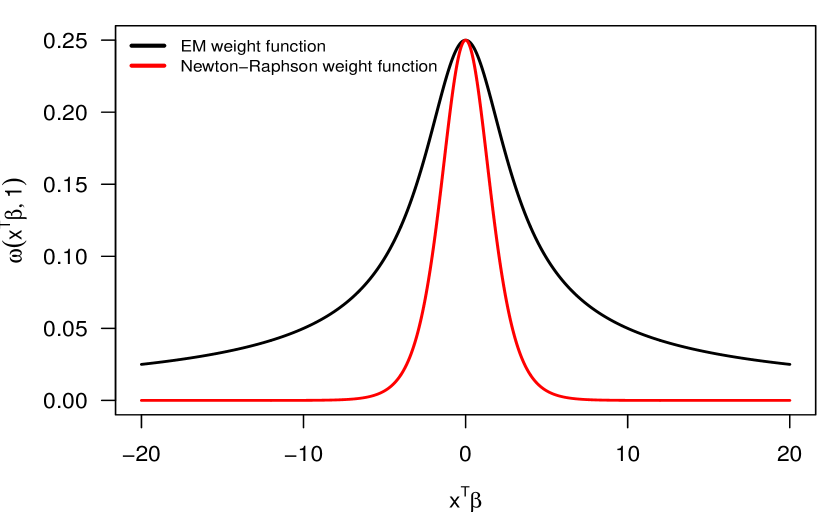
Figure 1: (Color Figure) Weight functions $\omega(\mathbf{x}^{T}\mbox{\boldmath$\beta$},m)$ and $\omega^{NR}(\mathbf{x}^{T}\mbox{\boldmath$\beta$},m)$ used in the EM and Newton-Raphson algorithms respectively for $m=1$. This figure shows the considerably heavier tails of the EM algorithm weight function.

A main advantage of the EM algorithm over the Newton-Raphson algorithm is that the EM algorithm is monotone; namely, iterates from the EM algorithm are guaranteed to increase the weighted log-likelihood at every iteration and the iterates are guaranteed to converge to a fixed-point of the algorithm. It is interesting to note that the first iterations of the EM and Newton-Raphson are identical whenever all components of the initial iterate $\mbox{\boldmath$\beta$}^{(0)}$ are set to zero. This is a consequence of the fact that $\omega^{EM}(0,m_{i})=\omega^{NR}(0,m_{i})=m_{i}/4$. While the Newton-Raphson algorithm is not monotone and does not possess any global convergence guarantees, the fact that the first step of Newton-Raphson increases the value of the log-likelihood when setting $\mbox{\boldmath$\beta$}^{(0)}=\mathbf{0}$ is one reason for the relatively robust performance of Newton-Raphson for logistic regression. The monotonicity of the Newton-Raphson first step when setting $\mbox{\boldmath$\beta$}^{(0)}=\mathbf{0}$ was also noted in Böhning & Lindsay (1988).

3 A Parameter-Expanded ECME Algorithm for Logistic Regression

3.1 Review of Parameter-Expanded EM and ECME Algorithms

In a variety of estimation problems, the convergence speed of the EM algorithm can be improved by viewing the complete-data model as embedded within a larger model that has additional parameters and then performing parameter updates with respect to the larger model. An EM algorithm constructed from a larger, parameter-expanded model is typically referred to as a parameter-expanded EM algorithm (PX-EM) algorithm (Liu et al. (1998)).

To describe the steps involved in the PX-EM algorithm, we consider a general setup where one is interested in estimating a parameter vector $\mbox{\boldmath$\beta$}\in\mathcal{B}$ and one has defined a complete-data vector $\mathbf{v}$ with density function $g_{c}(\mathbf{v}|\mbox{\boldmath$\beta$})$. The complete-data vector $\mathbf{v}\in\mathcal{V}$ and observed-data vector $\mathbf{y}\in\mathcal{Y}$ are connected through $\mathbf{y}=h(\mathbf{v})$ where $h:\mathcal{V}\longrightarrow\mathcal{Y}$ is the data-reducing mapping to be used for developing the EM algorithm. As described in Liu et al. (1998), to generate a PX-EM algorithm one must first consider an expanded probability model for the complete-data vector $\mathbf{v}$, and we let $g_{PX}(\mathbf{v}|\mbox{\boldmath$\theta$},\alpha)$ denote the probability density function for this expanded probability model where $(\mbox{\boldmath$\theta$},\alpha)$ are the parameters of the expanded model and $\Theta$ denotes the parameter space for $(\mbox{\boldmath$\theta$},\alpha)$. As outlined in Liu et al. (1998) and Lewandowski et al. (2010), the expanded probability model should satisfy the following conditions in order to generate a well-defined PX-EM algorithm

1. The observed-data model is preserved in the sense that there is a many-to-one reduction function $R:\Theta\longrightarrow\mathcal{B}$ such that

   $$g_{O}\big{\{}\mathbf{y}|\mbox{\boldmath$\beta$}=R(\mbox{\boldmath$\theta$},\alpha)\big{\}}=\int_{\mathcal{V}(\mathbf{y})}g_{PX}(\mathbf{v}|\mbox{\boldmath$\theta$},\alpha)d\mathbf{v},\quad\textrm{ for all }(\mbox{\boldmath$\theta$},\alpha)\in\Theta,$$

   where $\mathcal{V}(\mathbf{y})=\{\mathbf{v}\in\mathcal{V}:h(\mathbf{v})=\mathbf{y}\}$.

2. There is a “null value” $\alpha_{0}$ of $\alpha$ such that the complete-data model is preserved at the null value in the sense that

   $$g_{PX}(\mathbf{v}|\mbox{\boldmath$\beta$},\alpha_{0})=g_{c}(\mathbf{v}|\mbox{\boldmath$\beta$}),\qquad\textrm{for all }\mbox{\boldmath$\beta$}\in\mathcal{B}.$$

Similar to the EM algorithm, the PX-EM algorithm consists of two steps: a “PX–E” step followed by a “PX–M” step. The PX–E step is similar to the usual “E–step” of an EM algorithm in that a “Q-function” is formed by taking the expectation of the (parameter-expanded) complete-data log likelihood conditional on the observed data and parameter values $(\mbox{\boldmath$\theta$},\alpha)=(\mbox{\boldmath$\beta$}^{(t)},\alpha_{0})$. The “PX–M” step then proceeds by finding the expanded parameter values $(\mbox{\boldmath$\theta$}^{(t+1)},\alpha^{(t+1)})$ which maximize this Q-function and computing the parameter update $\mbox{\boldmath$\beta$}^{(t+1)}$ by applying the reduction function to $(\mbox{\boldmath$\theta$}^{(t+1)},\alpha^{(t+1)})$. The two steps of the PX-EM algorithm can be summarized as:

1. PX–E step: Compute the parameter-expanded Q-function

   $$Q_{PX}(\mbox{\boldmath$\theta$},\alpha|\mbox{\boldmath$\beta$}^{(t)},\alpha_{0})=E\Big{\{}\log g_{PX}(\mathbf{v}|\mbox{\boldmath$\theta$},\alpha)\Big{|}\mathbf{y},\mbox{\boldmath$\theta$}=\mbox{\boldmath$\beta$}^{(t)},\alpha=\alpha_{0}\Big{\}}.$$ (7)

2. PX–M step: Find

   $$(\mbox{\boldmath$\theta$}^{(t+1)},\alpha^{(t+1)})=\operatorname*{arg\,max}_{\boldsymbol{\theta,\alpha}}Q_{PX}(\mbox{\boldmath$\theta$},\alpha|\mbox{\boldmath$\beta$}^{(t)},\alpha_{0}),$$

   and update $\mbox{\boldmath$\beta$}^{(t)}$ using

   $$\mbox{\boldmath$\beta$}^{(t+1)}=R(\mbox{\boldmath$\theta$}^{(t+1)},\alpha^{(t+1)}).$$

A chief advantage of the PX-EM algorithm is that it is guaranteed to converge at least as fast as the corresponding EM algorithm. When the parameter-expanded model is constructed so that all parameter updates have a direct, closed-form, the PX-EM algorithm can have substantially faster convergence speed than the EM algorithm while maintaining the stability and computational simplicity of the original EM algorithm.

The Expectation-Conditional Maximization (ECM) algorithm (Meng & Rubin (1993)) and the Expectation-Conditional Maximization Either (ECME) algorithms (Liu & Rubin (1994)) are variations of the EM algorithm where the M-step is replaced by a sequence of conditional maximization steps. In the ECM algorithm, one breaks up the maximization of the Q-function into several conditional maximization steps where, in each conditional maximization step, one only maximizes the Q-function with respect to a subset of the parameters while keeping the remaining parameter values fixed. In the ECME algorithm, one also performs a series of conditional maximization steps. However, in the ECME algorithm, some of the conditional maximization are performed with respect to the observed-data log-likelihood function while the remaining conditional maximization steps are performed with respect to the usual Q-function.

As in the original ECME algorithm, in a parameter-expanded version of ECME (PX-ECME), one performs a sequence of conditional maximization steps for the expanded parameters $(\mbox{\boldmath$\theta$},\alpha)$ with some of the conditional maximization steps being performed with respect to the parameter-expanded Q-function while the other conditional maximization steps are performed with respect to the observed-data log-likelihood function. Specifically, when using the observed-data log-likelihood function for conditional maximization one will maximize $\ell_{o,\mathbf{s}}\{R(\mbox{\boldmath$\theta$},\alpha)|\mathbf{y}\}$ with respect to the subset of parameters being maximized in that conditional maximization step. After all of the expanded parameters have been updated through the sequence of conditional maximization steps, the update for the parameter of interest $\beta$ is found by applying the reduction function $R(\cdot)$ to the updated expanded parameters.

One example of a PX-ECME algorithm is the procedure described in Liu (1997) for estimating the parameters of a multivariate-t distribution. Here, the EM algorithm exploits the representation of the multivariate-t distribution as a scale mixture of multivariate normal distributions, and the parameter-expanded model utilized by Liu (1997) includes an expanded scale parameter that plays a role in both the covariance matrix of the normal distribution and the scale of the latent Gamma distribution. This expanded parameter is updated in each iteration through a conditional maximization step maximizing the observed-data likelihood.

One point worth noting is that a PX-ECME algorithm can often be constructed even if the expanded parameter vector $(\mbox{\boldmath$\theta$},\alpha)$ is not identifiable from the complete data. A PX-ECME algorithm can work if the subsets of parameters used in each conditional maximization step are conditionally identifiable from the observed data. Specifically, the parameters in each of the subsets should be identifiable from the observed data assuming that all the other parameters are fixed. For example, if we construct our PX-ECME algorithm so that $\theta$ is updated first followed by an update of $\alpha$, then $\theta$ should be identifiable for a fixed value of $\alpha$, and $\alpha$ should be identifiable from the observed data for a fixed value of $\theta$.

3.2 A Parameter-Expanded ECME Algorithm for Logistic and Penalized Logistic Regression

We consider the following parameter-expanded version of model (3) for the complete-data vector $\mathbf{v}=\{(y_{1},W_{1}),\ldots,(y_{n},W_{n})\}$

$$y_{i}|W_{i} \sim \textrm{Binomial}\Big{(}m_{i},\{1+\exp(-\alpha\mathbf{x}_{i}^{T}\mbox{\boldmath$\theta$})\}^{-1}\Big{)}$$

$$W_{i} \sim PG(m_{i},\alpha\mathbf{x}_{i}^{T}\mbox{\boldmath$\theta$}),$$ (8)

where the parameters in this model are $\mbox{\boldmath$\theta$}\in\mathbb{R}^{p}$ and $\alpha\in\mathbb{R}$. Under this expanded model, the observed-data model is preserved when using the reduction function $\mbox{\boldmath$\beta$}=R(\mbox{\boldmath$\theta$},\alpha)=\alpha\mbox{\boldmath$\theta$}$, and the original complete-data model (3) is preserved whenever $\alpha=\alpha_{0}=1$.

We now turn to describing how to use the parameter-expanded model (8) to construct a PX-ECME algorithm for maximizing a penalized weighted log-likelihood function with penalty function $P_{\boldsymbol{\eta}}(\mbox{\boldmath$\beta$})$. A PX-ECME algorithm for maximizing a penalized log-likelihood is very similar to that of maximizing a log-likelihood function the only difference being that a penalty function will be subtracted from either the parameter-expanded Q-function or the observed-data log-likelihood function. Throughout the remainder of this paper, we will assume the penalty function has the form $P_{\boldsymbol{\eta}}(\mbox{\boldmath$\beta$})=\sum_{j=1}^{p}P_{\boldsymbol{\eta},j}(\beta_{j})$, where $\mbox{\boldmath$\eta$}\in\mathbb{R}^{q}$ is a vector of tuning parameters. The observed-data weighted penalized log-likelihood function $p\ell_{o,\mathbf{s}}^{\boldsymbol{\eta}}$ that we seek to maximize is then

$$p\ell_{o,\mathbf{s}}^{\boldsymbol{\eta}}(\mbox{\boldmath$\beta$}|\mathbf{y})=\sum_{i=1}^{n}s_{i}\log\binom{m_{i}}{y_{i}}+\sum_{i=1}^{n}s_{i}y_{i}\mathbf{x}_{i}^{T}\mbox{\boldmath$\beta$}-\sum_{i=1}^{n}s_{i}m_{i}\log\Big{(}1+\exp\{\mathbf{x}_{i}^{T}\mbox{\boldmath$\beta$}\}\Big{)}-P_{\boldsymbol{\eta}}(\mbox{\boldmath$\beta$}),$$

and the complete-data penalized weighted log-likelihood corresponding to model (8) is

$$p\ell_{c,PX}^{\boldsymbol{\eta}}(\mbox{\boldmath$\theta$},\alpha|\mathbf{v})=\alpha\sum_{i=1}^{n}s_{i}u_{i}\mathbf{x}_{i}^{T}\mbox{\boldmath$\theta$}-\frac{\alpha^{2}}{2}\sum_{i=1}^{n}s_{i}W_{i}(\mathbf{x}_{i}^{T}\mbox{\boldmath$\theta$})^{2}-P_{\boldsymbol{\eta}}(\alpha\mbox{\boldmath$\theta$})+C,$$

where $C$ is a constant that does not depend on $(\mbox{\boldmath$\theta$},\alpha)$. The penalized, parameter-expanded Q-function $Q_{PX}^{\boldsymbol{\eta}}(\mbox{\boldmath$\theta$},\alpha|\mbox{\boldmath$\beta$}^{(t)},\alpha_{0})$ is obtained by just subtracting $P_{\boldsymbol{\eta}}(\alpha\mbox{\boldmath$\theta$})$ from the usual parameter-expanded Q-function (7). For model (8), this is given by

$$Q_{PX}^{\boldsymbol{\eta}}(\mbox{\boldmath$\theta$},\alpha|\mbox{\boldmath$\beta$}^{(t)},\alpha_{0})=\alpha\mbox{\boldmath$\theta$}^{T}\mathbf{X}^{T}\mathbf{S}\mathbf{u}-\frac{\alpha^{2}}{2}\mbox{\boldmath$\theta$}^{T}\mathbf{X}^{T}\mathbf{S}\mathbf{W}(\mbox{\boldmath$\beta$}^{(t)})\mathbf{X}\mbox{\boldmath$\theta$}-P_{\boldsymbol{\eta}}(\alpha\mbox{\boldmath$\theta$})+C,$$ (9)

where $\mathbf{W}(\mbox{\boldmath$\beta$}^{(t)})$ is the $n\times n$ weight matrix defined in (5).

One feature of the parameter-expanded model (8) is that the parameter vector $(\mbox{\boldmath$\theta$},\alpha)$ is not identifiable from the complete-data vector $\mathbf{v}$. This may be seen by noting that, for a positive scalar c, the parameters $(\alpha,\mbox{\boldmath$\theta$})$ and $(\alpha/c,c\mbox{\boldmath$\theta$})$ both lead to the same complete-data penalized log-likelihood. Nevertheless, $(\mbox{\boldmath$\theta$},\alpha)$ are conditionally identifiable meaning that, for a fixed $\theta$, $\alpha$ is identifiable, and for a fixed $\alpha$, $\theta$ is identifiable. Hence, we can first update $\mbox{\boldmath$\theta$}^{(t)}$ by fixing $\alpha=\alpha^{(t)}$ and maximizing $Q_{PX}^{\boldsymbol{\eta}}(\mbox{\boldmath$\theta$},\alpha|\mbox{\boldmath$\beta$}^{(t)},\alpha_{0})$ with respect to $\theta$

$$\mbox{\boldmath$\theta$}^{(t+1)} = \operatorname*{arg\,max}_{\boldsymbol{\theta}\in\mathbb{R}^{p}}Q_{PX}^{\boldsymbol{\eta}}(\mbox{\boldmath$\theta$},\alpha^{(t)}|\mbox{\boldmath$\beta$}^{(t)},\alpha_{0})$$ (10)

$$= \operatorname*{arg\,min}_{\boldsymbol{\theta}\in\mathbb{R}^{p}}\Bigg{[}-\alpha^{(t)}\mbox{\boldmath$\theta$}^{T}\mathbf{X}^{T}\mathbf{S}\mathbf{u}+\frac{(\alpha^{(t)})^{2}}{2}\mbox{\boldmath$\theta$}^{T}\mathbf{X}^{T}\mathbf{S}\mathbf{W}(\mbox{\boldmath$\beta$}^{(t)})\mathbf{X}\mbox{\boldmath$\theta$}+P_{\boldsymbol{\eta}}(\alpha^{(t)}\mbox{\boldmath$\theta$})-C\Bigg{]}.$$

We then update $\alpha^{(t)}$ by maximizing the observed-data penalized log-likelihood

$$\alpha^{(t+1)}=\operatorname*{arg\,max}_{\alpha\in\mathbb{R}}p\ell_{o}^{\boldsymbol{\eta}}(\alpha\mbox{\boldmath$\theta$}^{(t+1)}|\mathbf{y}).$$

The PX-ECME parameter update of $\mbox{\boldmath$\beta$}^{(t)}$ is given by $\mbox{\boldmath$\beta$}^{(t+1)}=R(\mbox{\boldmath$\theta$}^{(t+1)},\alpha^{(t+1)})=\alpha^{(t+1)}\mbox{\boldmath$\theta$}^{(t+1)}$.

It is worth noting that one can express $\mbox{\boldmath$\theta$}^{(t+1)}$ in terms of the EM parameter update as $\mbox{\boldmath$\theta$}^{(t+1)}=\mbox{\boldmath$\beta$}^{(t+1),EM}/\alpha^{(t)}$ where the EM update $\mbox{\boldmath$\beta$}^{(t+1),EM}$ is obtained from $\mbox{\boldmath$\beta$}^{(t)}$ by maximizing $Q_{PX}^{\boldsymbol{\eta}}(\mbox{\boldmath$\theta$},1|\mbox{\boldmath$\beta$}^{(t)},1)$ with respect to $\theta$. Hence, we can express the PX-ECME update as

$$\mbox{\boldmath$\beta$}^{(t+1)}=\frac{1}{\alpha^{(t)}}\mbox{\boldmath$\beta$}^{(t+1),EM}\Big{[}\operatorname*{arg\,max}_{\alpha\in\mathbb{R}}p\ell_{o,\mathbf{s}}^{\boldsymbol{\eta}}(\alpha\mbox{\boldmath$\beta$}^{(t+1),EM}/\alpha^{(t)}|\mathbf{y})\Big{]}=\rho^{(t+1)}\mbox{\boldmath$\beta$}^{(t+1),EM},$$

where $\rho^{(t+1)}=\operatorname*{arg\,max}_{\rho\in\mathbb{R}}p\ell_{o,\mathbf{s}}^{\boldsymbol{\eta}}(\rho\mbox{\boldmath$\beta$}^{(t+1),EM}|\mathbf{y})$. In other words, the PX-ECME update is found by simply first computing the EM update $\mbox{\boldmath$\beta$}^{(t+1),EM}$ of the regression coefficients and then multiplying $\mbox{\boldmath$\beta$}^{(t+1),EM}$ by the scaling factor $\rho^{(t+1)}$, where $\rho^{(t+1)}$ is the scalar maximizing the weighted observed-data penalized log-likelihood function among regression coefficients of the form $\rho\mbox{\boldmath$\beta$}^{(t+1),EM}$. The complete PX-ECME procedure is summarized in Algorithm 1.

Finding $\rho^{(t+1)}$ only involves solving a one-dimensional root-finding problem, namely, $\partial p\ell_{o,\mathbf{s}}^{\boldsymbol{\eta}}(\rho\mbox{\boldmath$\beta$}^{(t+1),EM}|\mathbf{y})/\partial\rho=0$, of which there are a wide range of available numerical methods, and in such cases, robust root-finding methods such as Brent’s method (Brent (2013)) may be directly used to find $\rho^{(t+1)}$.

Algorithm 1 (PX-ECME for Penalized Logistic Regression). In the description of the algorithm, $\mathbf{S}=\textrm{diag}\{s_{1},\ldots,s_{n}\}$ and $\mathbf{u}=(u_{1},\ldots,u_{n})^{T}$, where $u_{i}=y_{i}-m_{i}/2$.

1:Given $\mbox{\boldmath$\beta$}^{(0)}\in\mathbb{R}^{p}$.

2:for t=0,1,2,… until convergence do

3:     Compute the $n\times n$ diagonal weight matrix $\mathbf{W}(\mbox{\boldmath$\beta$}^{(t)})$ whose $i^{th}$ diagonal element is

$$\omega(\mathbf{x}_{i}^{T}\mbox{\boldmath$\beta$},m_{i})=\frac{m_{i}}{2\mathbf{x}_{i}^{T}\mbox{\boldmath$\beta$}^{(t)}}\tanh\big{(}\mathbf{x}_{i}^{T}\mbox{\boldmath$\beta$}^{(t)}/2\big{)}.$$

4:     Compute $\mbox{\boldmath$\beta$}^{(t+1),EM}$:

$$\mbox{\boldmath$\beta$}^{(t+1),EM}=\operatorname*{arg\,min}_{\boldsymbol{\beta}\in\mathbb{R}^{p}}\Big{[}\frac{1}{2}\mbox{\boldmath$\beta$}^{T}\mathbf{X}^{T}\mathbf{S}\mathbf{W}(\mbox{\boldmath$\beta$}^{(t)})\mathbf{X}\mbox{\boldmath$\beta$}-\mbox{\boldmath$\beta$}^{T}\mathbf{X}^{T}\mathbf{S}\mathbf{u}+P_{\boldsymbol{\eta}}(\mbox{\boldmath$\beta$})\Big{]}.\vspace{-.2cm}$$

5:     Compute

$$\rho^{(t+1)}=\operatorname*{arg\,max}_{\rho\in\mathbb{R}}\Big{[}p\ell_{o,\mathbf{s}}^{\boldsymbol{\eta}}(\rho\mbox{\boldmath$\beta$}^{(t+1),EM}|\mathbf{y})\Big{]}.$$

6:     Set $\mbox{\boldmath$\beta$}^{(t+1)}=\rho^{(t+1)}\mbox{\boldmath$\beta$}^{(t+1),EM}$.

An attractive feature of the PX-ECME algorithm (Algorithm 1) is that it is, like the EM algorithm, a monotone algorithm. The monotonicity property helps to ensure that the procedure stable and robust in practice. The monotonicity of PX-ECME directly follows from the fact that the EM algorithm is monotone with respect to the penalized log-likelihood (i.e., $p\ell_{o,\mathbf{s}}^{\boldsymbol{\eta}}(\mbox{\boldmath$\beta$}^{(t+1),EM}|\mathbf{y})\geq p\ell_{o,\mathbf{s}}^{\boldsymbol{\eta}}(\mbox{\boldmath$\beta$}^{(t)}|\mathbf{y})$) and that $p\ell_{o,\mathbf{s}}^{\boldsymbol{\eta}}(\rho^{(t+1)}\mbox{\boldmath$\beta$}^{(t+1),EM}|\mathbf{y})\geq p\ell_{o,\mathbf{s}}^{\boldsymbol{\eta}}(\mbox{\boldmath$\beta$}^{(t+1),EM}|\mathbf{y})$.

3.3 Monotone acceleration of EM via order-1 Anderson acceleration

The PX-ECME algorithm accelerates convergence by multiplying the EM parameter update by a single scalar, and there are likely other straightforward modifications of the EM algorithm that can produce substantial speed-ups in convergence without sacrificing the monotonicity property.

An attractive class of methods with straightforward parameter updates are those that simply take a linear combination of the previous two EM parameter updates with the weights in the linear combination determined adaptively. One can ensure that this scheme is monotone by comparing the value of the objective function for a parameter update versus that of the current parameter value. One method for finding the weights in this linear combination is the order-1 Anderson acceleration (Walker & Ni (2011)). Applying the order-1 Anderson acceleration to the EM algorithm for penalized logistic regression leads to the following parameter updating scheme

$$\mbox{\boldmath$\beta$}^{(t+1)}=\begin{cases}(1-\gamma^{(t)})\mbox{\boldmath$\beta$}^{(t+1),EM}+\gamma^{(t)}\mbox{\boldmath$\beta$}^{(t),EM}&\text{ if $p\ell_{o,\mathbf{s}}^{\boldsymbol{\eta}}(\mbox{\boldmath$\beta$}^{(t+1)}|\mathbf{y})\geq p\ell_{o,\mathbf{s}}^{\boldsymbol{\eta}}(\mbox{\boldmath$\beta$}^{(t+1),EM}|\mathbf{y})$ }\\ \mbox{\boldmath$\beta$}^{(t+1),EM}&\text{ otherwise, }\end{cases}$$

where $\gamma^{(t)}$ is the scalar $\gamma^{(t)}=\mathbf{v}_{t}^{T}\mathbf{r}_{t}/\mathbf{v}_{t}^{T}\mathbf{v}_{t}$ and where $\mathbf{r}_{t}=\mbox{\boldmath$\beta$}^{(t+1),EM}-\mbox{\boldmath$\beta$}^{(t)}$ and $\mathbf{v}_{t}=\mbox{\boldmath$\beta$}^{(t+1),EM}-\mbox{\boldmath$\beta$}^{(t)}+\mbox{\boldmath$\beta$}^{(t-1)}-\mbox{\boldmath$\beta$}^{(t),EM}$. Because the underlying EM algorithm is monotone, only accepting the linear combination $\mbox{\boldmath$\beta$}^{(t+1)}$ if $p\ell_{o,\mathbf{s}}^{\boldsymbol{\eta}}(\mbox{\boldmath$\beta$}^{(t+1)}|\mathbf{y})\geq p\ell_{o,\mathbf{s}}^{\boldsymbol{\eta}}(\mbox{\boldmath$\beta$}^{(t+1),EM}|\mathbf{y})$ ensures that the above iterative scheme is monotone.

3.4 Rate of Convergence of EM and PX-ECME for Logistic Regression

The PX-ECME updating scheme outlined in Algorithm 1 implicitly defines a mapping $G:\mathbb{R}^{p}\longrightarrow\mathbb{R}^{p}$ which performs the PX-ECME update of $\mbox{\boldmath$\beta$}^{(t)}$, i.e., $\mbox{\boldmath$\beta$}^{(t+1)}=G_{PX}(\mbox{\boldmath$\beta$}^{(t)})$. Likewise, the EM algorithm also defines a mapping $\mbox{\boldmath$\beta$}^{(t+1),EM}=G_{EM}(\mbox{\boldmath$\beta$}^{(t),EM})$ which, from (6), has the form $G_{EM}(\mbox{\boldmath$\beta$})=(\mathbf{X}^{T}\mathbf{S}\mathbf{W}(\mbox{\boldmath$\beta$})\mathbf{X})^{-1}\mathbf{X}^{T}\mathbf{S}\mathbf{u}$. Because the PX-ECME parameter update is a scalar multiple of the EM update, we can express the mapping $G_{PX}$ in terms of $G_{EM}$ as

$$G_{PX}(\mbox{\boldmath$\beta$})=h\{G_{EM}(\mbox{\boldmath$\beta$})\}G_{EM}(\mbox{\boldmath$\beta$}),$$ (11)

where $h:\mathbb{R}^{p}\longrightarrow\mathbb{R}$ is the function defined as $h(\mbox{\boldmath$\beta$})=\operatorname*{arg\,max}_{\rho}[p\ell_{o,\mathbf{s}}^{\boldsymbol{\eta}}(\rho\mbox{\boldmath$\beta$}|\mathbf{y})]$.

The rate of convergence of a fixed-point iteration of the form $\mbox{\boldmath$\beta$}^{(t+1)}=G(\mbox{\boldmath$\beta$}^{(t)})$ is typically defined as the maximum eigenvalue of the Jacobian matrix of $G$ when the Jacobian is evaluated at the convergence point $\mbox{\boldmath$\beta$}^{*}$ of the algorithm (see, e.g., McLachlan & Krishnan (2007)). As shown in Durante & Rigon (2018), the Jacobian matrix $\mathbf{J}_{EM}(\mbox{\boldmath$\beta$})$ associated with the mapping $G_{EM}(\mbox{\boldmath$\beta$})=(\mathbf{X}^{T}\mathbf{S}\mathbf{W}(\mbox{\boldmath$\beta$})\mathbf{X})^{-1}\mathbf{X}^{T}\mathbf{S}\mathbf{u}$ is given by

$$\mathbf{J}_{EM}(\mbox{\boldmath$\beta$})=\mathbf{I}_{p}-(\mathbf{X}^{T}\mathbf{S}\mathbf{W}(\mbox{\boldmath$\beta$})\mathbf{X})^{-1}\mathbf{X}^{T}\mathbf{S}\mathbf{R}(\mbox{\boldmath$\beta$})\mathbf{X},$$ (12)

where $\mathbf{R}(\mbox{\boldmath$\beta$})$ is the $n\times n$ diagonal matrix whose $i^{th}$ diagonal element is $m_{i}\pi(\mathbf{x}_{i}^{T}\mbox{\boldmath$\beta$})[1-\pi(\mathbf{x}_{i}^{T}\mbox{\boldmath$\beta$})]$ and $\pi(u)=1/\{1+\exp(-u)\}$. As we show in Theorem 1 below, the maximum eigenvalue of the Jacobian matrix of $G_{PX}$ at $\mbox{\boldmath$\beta$}^{*}$ can be no larger than the maximum eigenvalue of $\mathbf{J}_{EM}(\mbox{\boldmath$\beta$}^{*})$, and hence the rate of convergence of PX-ECME is no slower than the EM algorithm.

Theorem 1

When assuming the penalty function equals zero for all $\beta$ (i.e., $P_{\boldsymbol{\eta}}(\mbox{\boldmath$\beta$})\equiv 0$) and $\mbox{\boldmath$\beta$}^{*}\neq\mathbf{0}$, the Jacobian $\mathbf{J}_{PX}(\mbox{\boldmath$\beta$})=\partial G_{PX}(\mbox{\boldmath$\beta$})/\partial\mbox{\boldmath$\beta$}$ of the PX-ECME mapping at $\mbox{\boldmath$\beta$}=\mbox{\boldmath$\beta$}^{*}$ is given by

$$\mathbf{J}_{PX}(\mbox{\boldmath$\beta$}^{*}) = \mathbf{I}_{p}-\mathbf{E}^{-1}(\mbox{\boldmath$\beta$}^{*})\mathbf{V}(\mbox{\boldmath$\beta$}^{*})-[c(\mbox{\boldmath$\beta$}^{*})]^{-1}\mbox{\boldmath$\beta$}^{*}(\mbox{\boldmath$\beta$}^{*})^{T}\mathbf{V}(\mbox{\boldmath$\beta$}^{*})\big{\{}\mathbf{V}^{-1}(\mbox{\boldmath$\beta$}^{*})-\mathbf{E}^{-1}(\mbox{\boldmath$\beta$}^{*})\big{\}}\mathbf{V}(\mbox{\boldmath$\beta$}^{*})^{T}$$

$$= \mathbf{J}_{EM}(\mbox{\boldmath$\beta$}^{*})-[c(\mbox{\boldmath$\beta$}^{*})]^{-1}\mbox{\boldmath$\beta$}^{*}(\mbox{\boldmath$\beta$}^{*})^{T}\mathbf{V}(\mbox{\boldmath$\beta$}^{*})\big{\{}\mathbf{V}^{-1}(\mbox{\boldmath$\beta$}^{*})-\mathbf{E}^{-1}(\mbox{\boldmath$\beta$}^{*})\big{\}}\mathbf{V}(\mbox{\boldmath$\beta$}^{*})^{T},$$

where $\mathbf{J}_{EM}(\mbox{\boldmath$\beta$}^{*})$ is the Jacobian matrix of the EM mapping at $\mbox{\boldmath$\beta$}=\mbox{\boldmath$\beta$}^{*}$, $c(\mbox{\boldmath$\beta$}^{*})=(\mbox{\boldmath$\beta$}^{*})^{T}\mathbf{X}^{T}\mathbf{S}\mathbf{R}(\mbox{\boldmath$\beta$}^{*})\mathbf{X}\mbox{\boldmath$\beta$}^{*}$, $\mathbf{E}(\mbox{\boldmath$\beta$}^{*})=\mathbf{X}^{T}\mathbf{S}\mathbf{W}(\mbox{\boldmath$\beta$}^{*})\mathbf{X}$, and $\mathbf{V}(\mbox{\boldmath$\beta$}^{*})=\mathbf{X}^{T}\mathbf{S}\mathbf{R}(\mbox{\boldmath$\beta$}^{*})\mathbf{X}$. In addition, we have $r_{PX}\leq r_{EM}$, where $r_{PX}$ and $r_{EM}$ are the maximal eigenvalues of $\mathbf{J}_{PX}(\mbox{\boldmath$\beta$}^{*})$ and $\mathbf{J}_{EM}(\mbox{\boldmath$\beta$}^{*})$ respectively.

4 A Generalized PX-ECME Algorithm for Logistic Regression

4.1 Description of the Aproach

For many penalty functions, the maximization in (10) does not yield an easily-computable solution and may require the use of a time-consuming iterative procedure to compute $\mbox{\boldmath$\theta$}^{(t+1)}$. To better handle such cases, we consider a generalized PX-ECME algorithm where $\mbox{\boldmath$\theta$}^{(t+1)}$ maximizes a more manageable, surrogate parameter-expanded Q-function. The more manageable surrogate Q-functions $\tilde{Q}_{PX}^{\boldsymbol{\eta}}(\mbox{\boldmath$\theta$},\alpha|\mbox{\boldmath$\beta$}^{(t)},\alpha_{0})$ are assumed to have the form

$$\tilde{Q}_{PX}^{\boldsymbol{\eta}}(\mbox{\boldmath$\theta$},\alpha|\mbox{\boldmath$\beta$}^{(t)},\alpha_{0})=Q_{PX}^{\boldsymbol{\eta}}(\mbox{\boldmath$\theta$},\alpha|\mbox{\boldmath$\beta$}^{(t)},\alpha_{0})-\frac{1}{2}(\alpha\mbox{\boldmath$\theta$}-\mbox{\boldmath$\beta$}^{(t)})^{T}\mathbf{H}^{(t)}(\alpha\mbox{\boldmath$\theta$}-\mbox{\boldmath$\beta$}^{(t)})$$

$$=\alpha\mbox{\boldmath$\theta$}^{T}[\mathbf{X}^{T}\mathbf{S}\mathbf{u}+\mathbf{H}^{(t)}\mbox{\boldmath$\beta$}^{(t)}]-\frac{\alpha^{2}}{2}\mbox{\boldmath$\theta$}^{T}\big{[}\mathbf{X}^{T}\mathbf{S}\mathbf{W}(\mbox{\boldmath$\beta$}^{(t)})\mathbf{X}+\mathbf{H}^{(t)}\big{]}\mbox{\boldmath$\theta$}-P_{\boldsymbol{\eta}}(\alpha\mbox{\boldmath$\theta$})+C,$$ (13)

where $\mathbf{H}^{(t)}$ is a positive semi-definite $p\times p$ matrix. As in the PX-ECME algorithm for penalized logistic regression, to update $\mbox{\boldmath$\beta$}^{(t)}$ one first finds $\mbox{\boldmath$\theta$}^{(t+1)}$ and $\alpha^{(t+1)}$ by performing two conditional maximization steps with respect to $\tilde{Q}_{PX}^{\boldsymbol{\eta}}$ and then sets $\mbox{\boldmath$\beta$}^{(t+1)}=\alpha^{(t+1)}\mbox{\boldmath$\theta$}^{(t+1)}$. We will refer to an algorithm which updates $\mbox{\boldmath$\beta$}^{(t)}$ in this manner as a generalized parameter-expanded ECME (GPX-ECME) algorithm for penalized weighted logistic regression.

The steps involved in a GPX-ECME are outlined in Algorithm 2. Notice in this Algorithm that, as in the case of a PX-ECME algorithm, the process of first computing $\mbox{\boldmath$\theta$}^{(t+1)}$ and $\alpha^{(t+1)}$ and then setting $\mbox{\boldmath$\beta$}^{(t+1)}=\alpha^{(t+1)}\mbox{\boldmath$\theta$}^{(t+1)}$ may be equivalently expressed as $\mbox{\boldmath$\beta$}^{(t+1)}=\rho^{(t+1)}\mbox{\boldmath$\beta$}^{(t+1),GEM}$, where $\mbox{\boldmath$\beta$}^{(t+1),GEM}$ maximizes $\tilde{Q}_{PX}^{\boldsymbol{\eta}}(\mbox{\boldmath$\beta$},1|\mbox{\boldmath$\beta$}^{(t)},\alpha_{0})$ and $\rho^{(t+1)}$ maximizes $p\ell_{o,\mathbf{s}}^{\boldsymbol{\eta}}(\rho\mbox{\boldmath$\beta$}^{(t+1),GEM}|\mathbf{y})$ with respect to $\rho\in\mathbb{R}$. As stated in the following proposition, as long as $\mathbf{H}^{(t)}$ is a positive semi-definite matrix for each $t$, each iterate generated from a GPX-ECME algorithm will increase the value of the penalized log-likelihood.

Proposition 1

If $\mathbf{H}^{(t)}$ is a positive semi-definite matrix for each $t$, then iterates $\mbox{\boldmath$\beta$}^{(0)},\mbox{\boldmath$\beta$}^{(1)},\mbox{\boldmath$\beta$}^{(2)},...$ produced by a GPX-ECME algorithm (Algorithm 2) increase the penalized log-likelihood function at each iteration. That is, for any $t\geq 0$,

$$p\ell_{o,\mathbf{s}}^{\boldsymbol{\eta}}(\mbox{\boldmath$\beta$}^{(t+1)}|\mathbf{y})\geq p\ell_{o,\mathbf{s}}^{\boldsymbol{\eta}}(\mbox{\boldmath$\beta$}^{(t)}|\mathbf{y}).$$

The main purpose for considering surrogate Q-functions of the form (13) in a GPX-ECME algorithm is to allow for more easily-computable parameter updates. A choice of $\mathbf{H}^{(t)}$ which typically ensures an easy-to-compute maximizer of $\tilde{Q}_{PX}^{\boldsymbol{\eta}}(\mbox{\boldmath$\beta$},1|\mbox{\boldmath$\beta$}^{(t)},\alpha_{0})$ is $\mathbf{H}^{(t)}=\mathbf{D}^{(t)}-\mathbf{X}^{T}\mathbf{S}\mathbf{W}(\mbox{\boldmath$\beta$}^{(t)})\mathbf{X}$, where $\mathbf{D}^{(t)}$ is a $p\times p$ diagonal matrix with nonnegative diagonal entries $d_{jj}^{(t)}$. When using a matrix $\mathbf{H}^{(t)}$ of this form, the surrogate Q-function (13) with arguments $(\mbox{\boldmath$\beta$},1)$ reduces to

$$\tilde{Q}_{PX}^{\boldsymbol{\eta}}(\mbox{\boldmath$\beta$},1|\mbox{\boldmath$\beta$}^{(t)},\alpha_{0})=\mbox{\boldmath$\beta$}^{T}[\mathbf{X}^{T}\mathbf{S}\mathbf{u}+\mathbf{a}_{t}]-\frac{1}{2}\mbox{\boldmath$\beta$}^{T}\mathbf{D}^{(t)}\mbox{\boldmath$\beta$}-P_{\boldsymbol{\eta}}(\mbox{\boldmath$\beta$})+C,$$ (14)

where $\mathbf{a}_{t}=[\mathbf{D}^{(t)}-\mathbf{X}^{T}\mathbf{S}\mathbf{W}(\mbox{\boldmath$\beta$}^{(t)})\mathbf{X}]\mbox{\boldmath$\beta$}^{(t)}$. Because $\mathbf{D}^{(t)}$ is diagonal, maximizing (14) is often straightforward as one can maximize each component $\beta_{j}$ of $\tilde{Q}_{PX}^{\boldsymbol{\eta}}(\mbox{\boldmath$\beta$},1|\mbox{\boldmath$\beta$}^{(t)},\alpha_{0})$ separately by maximizing a quadratic function plus the $j^{th}$ component of the penalty function $P_{\boldsymbol{\eta},j}(\beta_{j})$.

Algorithm 2 (GPX-ECME for Penalized Logistic Regression). In the description of the algorithm, $\mathbf{u}=(u_{1},\ldots,u_{n})^{T}$, where $u_{i}=y_{i}-m_{i}/2$.

1:Given $\mbox{\boldmath$\beta$}^{(0)}\in\mathbb{R}^{p}$.

2:for t=0,1,2,… until convergence do

3:     Compute the $n\times n$ diagonal weight matrix $\mathbf{W}(\mbox{\boldmath$\beta$}^{(t)})$ whose $i^{th}$ diagonal element is

$$\omega(\mathbf{x}_{i}^{T}\mbox{\boldmath$\beta$},m_{i})=\frac{m_{i}}{2\mathbf{x}_{i}^{T}\mbox{\boldmath$\beta$}^{(t)}}\tanh\big{(}\mathbf{x}_{i}^{T}\mbox{\boldmath$\beta$}^{(t)}/2\big{)}.$$

4:     Compute $\mbox{\boldmath$\beta$}^{(t+1),GEM}$:

$$\mbox{\boldmath$\beta$}^{(t+1),GEM}=\operatorname*{arg\,min}_{\boldsymbol{\beta}\in\mathbb{R}^{p}}\Big{[}\frac{1}{2}\mbox{\boldmath$\beta$}^{T}\mathbf{X}^{T}\mathbf{S}\mathbf{W}(\mbox{\boldmath$\beta$}^{(t)})\mathbf{X}\mbox{\boldmath$\beta$}-\mbox{\boldmath$\beta$}^{T}\mathbf{X}^{T}\mathbf{S}\mathbf{u}+\frac{1}{2}(\mbox{\boldmath$\beta$}-\mbox{\boldmath$\beta$}^{(t)})^{T}\mathbf{H}^{(t)}(\mbox{\boldmath$\beta$}-\mbox{\boldmath$\beta$}^{(t)})+P_{\boldsymbol{\eta}}(\mbox{\boldmath$\beta$})\Big{]}.\vspace{-.2cm}$$

5:     Compute

$$\rho^{(t+1)}=\operatorname*{arg\,max}_{\rho\in\mathbb{R}}\Bigg{[}p\ell_{o,\mathbf{s}}^{\boldsymbol{\eta}}(\rho\mbox{\boldmath$\beta$}^{(t+1),GEM}|\mathbf{y})\Bigg{]}.$$

6:     Set $\mbox{\boldmath$\beta$}^{(t+1)}=\rho^{(t+1)}\mbox{\boldmath$\beta$}^{(t+1),GEM}$.

If choosing $\mathbf{H}^{(t)}=\mathbf{D}^{(t)}-\mathbf{X}^{T}\mathbf{W}(\mbox{\boldmath$\beta$}^{(t)})\mathbf{X}$ and setting all the diagonal elements of $\mathbf{D}^{(t)}$ equal so that $\mathbf{D}^{(t)}=\kappa_{t}^{-1}\mathbf{I}_{p}$ for some $\kappa_{t}>0$, $\mathbf{H}^{(t)}$ will be positive semi-definite provided that $\kappa_{t}^{-1}\geq\lambda_{max}\big{(}\mathbf{X}^{T}\mathbf{S}\mathbf{W}(\mbox{\boldmath$\beta$}^{(t)})\mathbf{X}\big{)}$, where $\lambda_{max}\big{(}\mathbf{X}^{T}\mathbf{S}\mathbf{W}(\mbox{\boldmath$\beta$}^{(t)})\mathbf{X}\big{)}$ is the maximum eigenvalue of $\mathbf{X}^{T}\mathbf{S}\mathbf{W}(\mbox{\boldmath$\beta$}^{(t)})\mathbf{X}$. When using $\mathbf{D}^{(t)}=\kappa_{t}^{-1}\mathbf{I}_{p}$, it follows from (7) that the term $\mbox{\boldmath$\beta$}^{(t+1),GEM}$ computed in Step 4 of Algorithm 2 can be be expressed as

$$\mbox{\boldmath$\beta$}^{(t+1),GEM} = \operatorname*{arg\,min}_{\boldsymbol{\beta}\in\mathbb{R}^{p}}\Big{[}\frac{1}{2}\mbox{\boldmath$\beta$}^{T}\mbox{\boldmath$\beta$}-\kappa_{t}\mbox{\boldmath$\beta$}^{T}[\mathbf{X}^{T}\mathbf{S}\mathbf{u}+\mathbf{a}_{t}]+\kappa_{t}P_{\boldsymbol{\eta}}(\mbox{\boldmath$\beta$})\Big{]}.$$ (15)

Each component $\beta_{j}^{(t+1),GEM}$ of $\mbox{\boldmath$\beta$}^{(t+1),GEM}$ can be updated independently of the other components via

$$\beta_{j}^{(t+1),GEM}=\operatorname*{arg\,min}_{\beta_{j}\in\mathbb{R}}\Bigg{[}\frac{\beta_{j}^{2}}{\kappa_{t}}-2\Big{(}\sum_{i=1}^{n}x_{ij}s_{i}u_{i}+a_{j,t}\Big{)}\beta_{j}+2P_{\boldsymbol{\eta},j}(\beta_{j})\Bigg{]},$$ (16)

where $a_{j,t}$ denotes the $j^{th}$ component of $\mathbf{a}_{t}$.

The updates (16) have a closed form for a number of common penalty functions. For example, in the case of the elastic net penalty function where $P_{\boldsymbol{\eta},j}(\beta_{j})=\lambda_{1}|\beta_{j}|+\tfrac{\lambda_{2}}{2}\beta_{j}^{2}$, the update for the $j^{th}$ component of $\mbox{\boldmath$\beta$}^{(t)}$ is given by

$$\beta_{j}^{(t+1),GEM}=\begin{cases}\frac{1}{1/\kappa_{t}+\lambda_{2}}\Big{(}\sum_{i=1}^{n}x_{ij}s_{i}u_{i}+a_{j,t}-\lambda_{1}\Big{)}&\textrm{ if }\sum_{i=1}^{n}x_{ij}s_{i}u_{i}+a_{j,t}>\lambda_{1}\\ \frac{1}{1/\kappa_{t}+\lambda_{2}}\Big{(}\sum_{i=1}^{n}x_{ij}s_{i}u_{i}+a_{j,t}+\lambda_{1}\Big{)}&\textrm{ if }\sum_{i=1}^{n}x_{ij}s_{i}u_{i}+a_{j,t}<-\lambda_{1}\\ 0&\text{ if }\Big{|}\sum_{i=1}^{n}x_{ij}s_{i}u_{i}+a_{j,t}\Big{|}\leq\lambda_{1}\end{cases}$$

While other popular choices of the penalty function such as the smoothly clipped absolute deviation (SCAD) (Fan & Li (2001)) penalty may not necessarily yield direct, closed-form solutions, the parameter updates may be directly found by performing a univariate minimization separately for each component of the parameter vector.

4.2 Connections to Proximal Gradient Descent

Proximal gradient methods (Parikh & Boyd (2014)) are commonly used to optimize a function which can be expressed as the sum of a continuously differentiable function and a non-smooth function. In the context of penalized logistic regression where the aim is to minimize the composite function $p\ell_{o,\mathbf{s}}^{\boldsymbol{\eta}}(\mbox{\boldmath$\beta$}|\mathbf{y})=-\ell_{o,\mathbf{s}}(\mbox{\boldmath$\beta$}|\mathbf{y})+P_{\boldsymbol{\eta}}(\mbox{\boldmath$\beta$})$, the proximal gradient descent update with steplength $\kappa_{t}$ of a current parameter estimate $\mbox{\boldmath$\beta$}^{(t)}$ is given by

$$\mbox{\boldmath$\beta$}^{(t+1)}=\textrm{prox}_{\kappa_{t}P_{\boldsymbol{\eta}}}\Big{(}\mbox{\boldmath$\beta$}^{(t)}+\kappa_{t}\nabla\ell_{o,\mathbf{s}}(\mbox{\boldmath$\beta$}^{(t)}|\mathbf{y})\Big{)},$$ (17)

where the proximal operator $\textrm{prox}_{\kappa_{t}P_{\boldsymbol{\eta}}}:\mathbb{R}^{p}\longrightarrow\mathbb{R}^{p}$ of the function $\kappa_{t}P_{\boldsymbol{\eta}}$ is defined as

$$\textrm{prox}_{\kappa_{t}P_{\boldsymbol{\eta}}}(\mbox{\boldmath$\gamma$})=\operatorname*{arg\,min}_{\boldsymbol{\beta}}\Big{[}\frac{1}{2}\mbox{\boldmath$\beta$}^{T}\mbox{\boldmath$\beta$}-\mbox{\boldmath$\beta$}^{T}\mbox{\boldmath$\gamma$}+\kappa_{t}P_{\eta}(\mbox{\boldmath$\beta$})\Big{]}.$$

To elaborate on the connection between the proximal gradient update and the GPX-ECME procedure, we first note that the gradient of the observed-data log-likelihood function (2) is $\nabla\ell_{o,\mathbf{s}}(\mbox{\boldmath$\beta$}|\mathbf{y})=\mathbf{X}^{T}\mathbf{S}\{\mathbf{y}-\mu(\mathbf{X}\mbox{\boldmath$\beta$})\}$, where $\mu(\mathbf{X}\mbox{\boldmath$\beta$})$ is an $n\times 1$ vector whose $i^{th}$ component $[\mu(\mathbf{X}\mbox{\boldmath$\beta$})]_{i}$ is given by $[\mu(\mathbf{X}\mbox{\boldmath$\beta$})]_{i}=m_{i}\textrm{expit}(\mathbf{x}_{i}^{T}\mbox{\boldmath$\beta$})$. Using the connection (5) between the mean function $\mu(\mathbf{X}\mbox{\boldmath$\beta$})$ and the weight matrix $\mathbf{W}(\mbox{\boldmath$\beta$})$, we can write the gradient of $\ell_{o,\mathbf{s}}(\mbox{\boldmath$\beta$}|\mathbf{y})$ as

$$\nabla\ell_{o,\mathbf{s}}(\mbox{\boldmath$\beta$}|\mathbf{y})=\mathbf{X}^{T}\mathbf{S}\{\mathbf{u}-\mathbf{W}(\mbox{\boldmath$\beta$})\mathbf{X}\mbox{\boldmath$\beta$}\}.$$

Thus, the proximal gradient update (17) for penalized logistic can be expressed as

$$\mbox{\boldmath$\beta$}^{(t+1),PGD} = \textrm{prox}_{\kappa_{t}P_{\boldsymbol{\eta}}}\Big{(}\mbox{\boldmath$\beta$}^{(t)}+\kappa_{t}\mathbf{X}^{T}\mathbf{S}\{\mathbf{u}-\mathbf{W}(\mbox{\boldmath$\beta$}^{(t)})\mathbf{X}\mbox{\boldmath$\beta$}^{(t)}\}\Big{)}$$ (18)

$$= \operatorname*{arg\,min}_{\boldsymbol{\beta}\in\mathbb{R}^{p}}\Big{[}\frac{1}{2}\mbox{\boldmath$\beta$}^{T}\mbox{\boldmath$\beta$}-\mbox{\boldmath$\beta$}^{T}\Big{(}\mbox{\boldmath$\beta$}^{(t)}+\kappa_{t}\mathbf{X}^{T}\mathbf{S}\{\mathbf{u}-\mathbf{W}(\mbox{\boldmath$\beta$}^{(t)})\mathbf{X}\mbox{\boldmath$\beta$}^{(t)}\}\Big{)}+\kappa_{t}P_{\boldsymbol{\eta}}(\mbox{\boldmath$\beta$})\Big{]}.$$

It is interesting to note that the proximal gradient descent update (18) is exactly the same as the update $\mbox{\boldmath$\beta$}^{(t+1),GEM}$ in (15), which is part of a GPX-ECME algorithm with $\mathbf{H}^{(t)}=\kappa_{t}^{-1}\mathbf{I}_{p}-\mathbf{X}^{T}\mathbf{S}\mathbf{W}(\mbox{\boldmath$\beta$}^{(t)})\mathbf{X}$. In other words, the GPX-ECME algorithm with this choice of $\mathbf{H}^{(t)}$ may be interpreted as a proximal gradient descent algorithm where one first takes a proximal gradient descent step with steplength $\kappa_{t}$ and then multiplies this update by the optimal scalar $\rho^{(t+1)}$ which is optimal in the sense that it leads to the largest increase in the observed-data penalized log-likelihood.

4.3 Connection to an MM algorithm for Logistic Regression

If one chooses $\mathbf{H}^{(t)}$ to be $\mathbf{H}^{(t)}=\mathbf{X}^{T}\mathbf{S}[\kappa_{t}\mathbf{I}_{p}-\mathbf{W}(\mbox{\boldmath$\beta$}^{(t)})]\mathbf{X}$ for a positive scalar $\kappa_{t}>0$ in a GPX-ECME algorithm, the surrogate Q-function becomes

$$\tilde{Q}_{PX}^{\boldsymbol{\eta}}(\mbox{\boldmath$\beta$},1|\mbox{\boldmath$\beta$}^{(t)},\alpha_{0})=\mbox{\boldmath$\beta$}^{T}\mathbf{X}^{T}\mathbf{S}\mathbf{b}^{(t)}(\kappa_{t})-\frac{\kappa_{t}}{2}\mbox{\boldmath$\beta$}^{T}\mathbf{X}^{T}\mathbf{S}\mathbf{X}\mbox{\boldmath$\beta$}-P_{\boldsymbol{\eta}}(\mbox{\boldmath$\beta$})+C,$$ (19)

where $\mathbf{b}^{(t)}(\kappa_{t})=\mathbf{u}+[\kappa_{t}\mathbf{I}_{p}-\mathbf{W}(\mbox{\boldmath$\beta$}^{(t)})]\mathbf{X}\mbox{\boldmath$\beta$}^{(t)}$ and $C$ is a constant independent of $\beta$. In this context, the matrix $\mathbf{H}^{(t)}$ is guaranteed to be positive semi-definite if $\kappa_{t}$ greater than or equal to the largest diagonal element of $\mathbf{W}(\mbox{\boldmath$\beta$}^{(t)})$. For example, setting $\kappa_{t}=\kappa_{t}^{*}$ where

$$\kappa_{t}^{*}=\max\Big{\{}\omega(\mathbf{x}_{1}^{T}\mbox{\boldmath$\beta$}^{(t)},m_{1}),\ldots,\omega(\mathbf{x}_{n}^{T}\mbox{\boldmath$\beta$}^{(t)},m_{n})\Big{\}}$$

guarantees that $\mathbf{H}^{(t)}$ is positive semi-definite. When there is no penalty (i.e., $P_{\boldsymbol{\eta}}(\mbox{\boldmath$\beta$})=0$), maximizing $\tilde{Q}_{PX}^{\boldsymbol{\eta}}(\mbox{\boldmath$\beta$},1|\mbox{\boldmath$\beta$}^{(t)},\alpha_{0})$ with respect to $\beta$ leads to the following formula for $\mbox{\boldmath$\beta$}^{(t+1),GEM}$

$$\mbox{\boldmath$\beta$}^{(t+1),GEM}=\operatorname*{arg\,max}_{\boldsymbol{\beta}\in\mathbb{R}^{p}}\tilde{Q}_{PX}^{\boldsymbol{\eta}}(\mbox{\boldmath$\beta$},1|\mbox{\boldmath$\beta$}^{(t)},\alpha_{0})=\frac{1}{\kappa_{t}}(\mathbf{X}^{T}\mathbf{S}\mathbf{X})^{-1}\mathbf{X}^{T}\mathbf{S}\mathbf{b}^{(t)}(\kappa_{t}).$$ (20)

The update $\mbox{\boldmath$\beta$}^{(t+1)}$ is then found by finding $\rho^{(t+1)}=\operatorname*{arg\,max}_{\rho\in\mathbb{R}}p\ell_{o,\mathbf{s}}(\rho\mbox{\boldmath$\beta$}^{(t+1),GEM}|\mathbf{y})$ and setting $\mbox{\boldmath$\beta$}^{(t+1)}=\rho^{(t+1)}\mbox{\boldmath$\beta$}^{(t+1),GEM}$.

The algorithm defined by the update (20) is closely related to the MM algorithm for logistic regression described in Böhning & Lindsay (1988) and also detailed in Hunter & Lange (2004). To see why, if we use the fact that (5) implies

$$\mathbf{b}^{(t)}(\kappa_{t})=\mathbf{u}+\big{[}\kappa_{t}\mathbf{I}-\mathbf{W}(\mbox{\boldmath$\beta$}^{(t)})\big{]}\mathbf{X}\mbox{\boldmath$\beta$}^{(t)}=\kappa_{t}\mathbf{X}\mbox{\boldmath$\beta$}^{(t)}+\mathbf{y}-\mu(\mathbf{X}^{T}\mbox{\boldmath$\beta$}^{(t)}),$$

then (20) can be rewritten as

$$\mbox{\boldmath$\beta$}^{(t+1),GEM} = \mbox{\boldmath$\beta$}^{(t)}+\frac{1}{\kappa_{t}}(\mathbf{X}^{T}\mathbf{S}\mathbf{X})^{-1}\mathbf{X}^{T}\mathbf{S}\big{\{}\mathbf{y}-\mu(\mathbf{X}^{T}\mbox{\boldmath$\beta$}^{(t)})\big{\}}.$$ (21)

If we were to set $\kappa_{t}=1/4$ for each $t$ in (21), then in the case of $m_{1}=m_{2}=\ldots=m_{n}=1$, then (21) would correspond exactly to the MM algorithm for logistic regression update described by Böhning & Lindsay (1988). Note that, in the case when all $m_{i}$ equal $1$, setting $\kappa_{t}=1/4$ guarantees that $\mathbf{H}^{(t)}$ is positive semi-definite because $\omega(\mathbf{x}^{T}\mbox{\boldmath$\beta$},1)\leq 1/4$ for any value of $\mathbf{x}^{T}\mbox{\boldmath$\beta$}$. One advantage of using $\kappa_{t}=1/4$ rather than $\kappa_{t}=\kappa_{t}^{*}$ is that one does not need to compute the maximum of the weights in each iteration; however, this could result in taking slightly smaller “steps” when compared with using $\kappa_{t}^{*}$.

In the case of an $L_{2}$ penalty where $P_{\boldsymbol{\eta}}(\mbox{\boldmath$\beta$})=\tfrac{\lambda}{2}\sum_{j=1}^{p}\beta_{j}^{2}$, one would, in (21), simply replace $(\mathbf{X}^{T}\mathbf{S}\mathbf{X})^{-1}$ with the matrix $(\mathbf{X}^{T}\mathbf{S}\mathbf{X}+\tfrac{\lambda}{\kappa_{t}}\mathbf{I}_{p})^{-1}$. This approach for the $L_{2}$-penalized logistic regression problem, which we label the “PX-MM” algorithm is summarized in Algorithm 3.

Algorithm 3 (PX-MM algorithm for Logistic Regression with $L_{2}$ penalty $P_{\boldsymbol{\eta}}(\mbox{\boldmath$\beta$})=\frac{\lambda}{2}\mbox{\boldmath$\beta$}^{T}\mbox{\boldmath$\beta$}$). In the description of the algorithm, $\mathbf{u}=(u_{1},\ldots,u_{n})^{T}$, where $u_{i}=y_{i}-m_{i}/2$.

1:Given $\mbox{\boldmath$\beta$}^{(0)}\in\mathbb{R}^{p}$.

2:for t=0,1,2,… until convergence do

3:     Compute the $n\times n$ diagonal weight matrix $\mathbf{W}(\mbox{\boldmath$\beta$}^{(t)})$ whose $i^{th}$ diagonal element is

$$\omega(\mathbf{x}_{i}^{T}\mbox{\boldmath$\beta$},m_{i})=\frac{m_{i}}{2\mathbf{x}_{i}^{T}\mbox{\boldmath$\beta$}^{(t)}}\tanh\big{(}\mathbf{x}_{i}^{T}\mbox{\boldmath$\beta$}^{(t)}/2\big{)}.$$

4:     Set $\kappa_{t}^{*}=\max\big{\{}\omega(\mathbf{x}_{1}^{T}\mbox{\boldmath$\beta$}^{(t)},m_{1}),\ldots,\omega(\mathbf{x}_{n}^{T}\mbox{\boldmath$\beta$}^{(t)},m_{n})\big{\}}$.

5:     Compute $\mbox{\boldmath$\beta$}^{(t+1),GEM}$:

$$\mbox{\boldmath$\beta$}^{(t+1),GEM}=\big{(}\mathbf{X}^{T}\mathbf{S}\mathbf{X}+\tfrac{\lambda}{\kappa_{t}^{*}}\mathbf{I}_{p}\big{)}^{-1}\mathbf{X}^{T}\mathbf{S}\mathbf{X}\mbox{\boldmath$\beta$}^{(t)}+\frac{1}{\kappa_{t}^{*}}\big{(}\mathbf{X}^{T}\mathbf{S}\mathbf{X}+\tfrac{\lambda}{\kappa_{t}^{*}}\mathbf{I}_{p}\big{)}^{-1}\mathbf{X}^{T}\mathbf{S}\big{\{}\mathbf{y}-\mu(\mathbf{X}^{T}\mbox{\boldmath$\beta$}^{(t)})\big{\}}.\vspace{-.2cm}$$

6:     Compute

$$\rho^{(t+1)}=\operatorname*{arg\,max}_{\rho\in\mathbb{R}}\Big{[}p\ell_{o,\mathbf{s}}^{\boldsymbol{\eta}}(\rho\mbox{\boldmath$\beta$}^{(t+1),GEM}|\mathbf{y})\Big{]}.$$

7:     Set $\mbox{\boldmath$\beta$}^{(t+1)}=\rho^{(t+1)}\mbox{\boldmath$\beta$}^{(t+1),GEM}$.

5 PX-ECME and Coordinate Descent

Coordinate descent is often used in the context of $L_{1}$-penalized regression (Friedman et al. (2007)) and $L_{1}$-penalized generalized linear models (Friedman et al. (2010)). Coordinate descent proceeds by updating each regression coefficient one at a time while holding the remaining coefficients fixed. This is frequently an efficient approach as the parameter updates usually have a simple, closed form, and many of the parameters do not change after being mapped to zero.

One could also consider a coordinate descent version of the PX-ECME algorithm where one instead updates the elements of the vector $\theta$ one at a time rather than in a single step. To be more specific, consider the parameter-expanded Q-function defined in (9) with the “elastic net” penalty $P_{\boldsymbol{\eta},j}(\beta_{j})=\lambda_{1}|\beta_{j}|+\frac{\lambda_{2}}{2}\beta_{j}^{2}$ and where the first $j-1$ components of $\theta$ have already been updated

$$Q_{PX}^{\lambda}(\theta_{1}^{(t+1)},\ldots,\theta_{j-1}^{(t+1)},\theta_{j},\theta_{j+1}^{(t)},\ldots,\theta_{p}^{(t)},\alpha^{(t)}|\mbox{\boldmath$\theta$}^{(t)},\alpha^{(t)})=\alpha^{(t)}\theta_{j}\Big{(}\sum_{i=1}^{n}x_{ij}s_{i}u_{i}\Big{)}-$$ (22)

$$- \frac{(\alpha^{(t)})^{2}}{2}\Big{(}\theta_{j}^{2}\Big{\{}\sum_{i=1}^{n}(A_{ij}^{(t)})^{2}+\lambda_{2}\Big{\}}+2\theta_{j}\sum_{i=1}^{n}A_{ij}^{(t)}\sum_{k\neq j}\theta_{k}^{(t+j/p)}A_{ik}^{(t)}\Big{)}-|\alpha^{(t)}|\lambda_{1}|\theta_{j}|+\tilde{C},$$

where $A_{ij}^{(t)}$ denotes the $(i,j)$ element of $\mathbf{S}^{1/2}\mathbf{W}^{1/2}(\mbox{\boldmath$\beta$}^{(t)})\mathbf{X}$, $\tilde{C}$ is a constant not depending on $\theta_{j}$. Maximizing (22) with respect to $\theta_{j}$ leads to an update of $\theta_{j}^{(t)}$ which has the form

$$\theta_{j}^{(t+1)}=\textrm{sign}\Big{(}\tfrac{1}{\alpha^{(t)}}V_{j}(\mbox{\boldmath$\beta$}^{(t)})-U_{j}(\mbox{\boldmath$\beta$}^{(t)},\mbox{\boldmath$\theta$}_{-j}^{(t+j/p)})\Big{)}\max\Big{\{}\Big{|}\tfrac{1}{\alpha^{(t)}}V_{j}(\mbox{\boldmath$\beta$}^{(t)})-U_{j}(\mbox{\boldmath$\beta$}^{(t)},\mbox{\boldmath$\theta$}_{-j}^{(t+j/p)})\Big{|}-\tfrac{1}{\alpha^{(t)}}\tilde{\lambda}(\mbox{\boldmath$\beta$}^{(t)}),0\Big{\}}.$$ (23)

Expressions for the terms $V_{j}(\mbox{\boldmath$\beta$}^{(t)})$, $U_{j}(\mbox{\boldmath$\beta$}^{(t)},\mbox{\boldmath$\theta$}_{-j}^{(t+j/p)})$, and $\tilde{\lambda}(\mbox{\boldmath$\beta$}^{(t)})$ are given in Appendix C. After completing one “cycle” of coordinate descent where all $p$ components of $\theta$ are updated using (23), one can update the value of $\alpha^{(t)}$ by maximizing $p\ell_{o,\mathbf{s}}^{\boldsymbol{\eta}}(\alpha\mbox{\boldmath$\theta$}|\mathbf{y})$ with respect to $\alpha$. After completing this cycle, the regression coefficients would be updated via $\mbox{\boldmath$\beta$}^{(t+1)}=\alpha^{(t+1)}\mbox{\boldmath$\theta$}^{(t+1)}$.

Rather than waiting an entire cycle to update $\alpha^{(t)}$ and the weight matrix $\mathbf{W}(\mbox{\boldmath$\beta$}^{(t)})$, an alternative is to perform this updating after a “block” of $k$ of the components (for $k\leq p$) of $\mbox{\boldmath$\theta$}^{(t)}$ have been updated rather than all $p$ components. This can often reduce the total number of coordinate cycles required to converge; however, this comes at the expense of a greater computational cost to perform each coordinate descent cycle. The more general PX-ECME algorithm which updates the value of $\alpha$ and the regression weights after every $k$ coordinate updates is outlined in Algorithm 4 of Appendix C. Note that when $k=p$, this algorithm reduces to the case where $\alpha$ and the weight matrix are only updated after a full cycle of coordinate descent is completed.

Our experience with running the PX-ECME version of coordinate descent suggests that it typically offers very modest improvements in the total number of iterations compared to coordinate descent with no parameter expansion (i.e., $\alpha^{(t)}=1$ for all $t$), and the extra computational effort involved in updating $\alpha^{(t)}$ often nullifies any reduction in the total number of coordinate descent iterations. Nevertheless, experimenting with different values of the “block size” parameter $k$ can have a positive impact in some cases, and hence, in some settings, it may be worth exploring different values of $k$ to determine if there are any gains to be had over a “classic” coordinate descent algorithm which does not have any parameter expansion whatsoever.

6 Simulations

6.1 A Weighted Logistic Regression Example

In the standard logistic regression setting where all the weights $s_{i}$ are equal, the usual starting values used for the Newton-Raphson algorithm (i.e., $\mbox{\boldmath$\beta$}^{(0)}=\mathbf{0}$) are generally quite robust, and using these starting values with Newton-Raphson produces iterates which converge to the maximum likelihood estimates of the regression coefficients. However, in many weighted logistic regression problems where there is large variability in the weights, the Newton-Raphson algorithm can result in failure even when the starting values of $\mbox{\boldmath$\beta$}^{(0)}=\mathbf{0}$ are used. To illustrate this, we consider the following small numerical example with responses $y_{i}$, scalar covariates $x_{i}$, and regression weights $s_{i}$:

$$(y_{1},\ldots,y_{7}) = (1,0,1,1,1,0,1)$$

$$(x_{1},\ldots,x_{7}) = (0,0,0.001,100,-1,-1,0.5)$$

$$(s_{1},\ldots,s_{7}) = (0.4,0.01,0.4,0.01,0.04,0.1,0.04).$$ (24)

The performance of Newton-Raphson, PX-ECME, and EM using the data and regression weights in (24) and with no penalty term is summarized in Table 1. We ran each method for 63 iterations because this was the number of iterations required for PX-ECME to converge when using the stopping criterion $\sqrt{\sum_{j=1}^{p}(\beta_{j}^{(t+1)}-\beta_{j}^{(t)})^{2}}<10^{-9}$. As shown in Table 1, the Newton-Raphson procedure diverges even when using the starting values $\mbox{\boldmath$\beta$}^{(0)}=\mathbf{0}$. While the first iteration of Newton-Raphson improves the value of the weighted log-likelihood, the subsequent iterates begin to quickly diverge. In contrast to Newton-Raphson, the PX-ECME algorithm provides more stable monotone convergence to the weighted maximum likelihood estimates $(\hat{\beta}_{0},\hat{\beta}_{1})=(4.39,5.30)$. While the EM algorithm also enjoys monotone convergence, the convergence is considerably slower than PX-EMCE, and it takes $419$ iterations for EM to converge when using the same convergence tolerance as PX-ECME.

	Newton-Raphson			PX-ECME			EM
k	$\beta_{0}^{(k)}$	$\beta_{1}^{(k)}$	$\ell_{o,\mathbf{s}}^{(k)}$	$\beta_{0}^{(k)}$	$\beta_{1}^{(k)}$	$\ell_{o,\mathbf{s}}^{(k)}$	$\beta_{0}^{(k)}$	$\beta_{1}^{(k)}$	$\ell_{o,\mathbf{s}}^{(k)}$
0	0.0	0.0	-0.6931	0.0	0.0	-0.6931	0.0	0.0	-0.6931
1	4.26	1.97	-0.2972	1.55	0.01	-0.3611	1.55	0.01	-0.3611
2	-79.22	-10.17	-80.4768	2.09	0.02	-0.3441	1.85	0.01	-0.3471
3	$1.87\times 10^{16}$	$4.31\times 10^{15}$	$-1.62\times 10^{15}$	2.10	0.03	-0.3432	1.97	0.02	-0.3441
4	$9.60\times 10^{15}$	$4.43\times 10^{15}$	$-6.13\times 10^{14}$	2.10	0.03	-0.3424	2.03	0.03	-0.3429
5	$4.88\times 10^{14}$	$4.56\times 10^{15}$	$-1.67\times 10^{14}$	2.10	0.05	-0.3414	2.05	0.04	-0.3420
6	$5.28\times 10^{14}$	$4.51\times 10^{15}$	$-1.64\times 10^{14}$	2.11	0.06	-0.3404	2.07	0.05	-0.3410
7	$5.68\times 10^{14}$	$4.46\times 10^{15}$	$-1.61\times 10^{14}$	2.12	0.07	-0.3392	2.07	0.06	-0.3400
8	$6.08\times 10^{14}$	$4.42\times 10^{15}$	$-1.58\times 10^{14}$	2.13	0.09	-0.3377	2.08	0.08	-0.3388
9	$6.48\times 10^{14}$	$4.37\times 10^{15}$	$-1.55\times 10^{14}$	2.14	0.11	-0.3360	2.08	0.09	-0.3373
10	$6.88\times 10^{14}$	$4.33\times 10^{15}$	$-1.52\times 10^{14}$	2.15	0.14	-0.3339	2.08	0.11	-0.3357
⋮	⋮	⋮	⋮	⋮	⋮	⋮	⋮	⋮	⋮
⋮	⋮	⋮	⋮	⋮	⋮	⋮	⋮	⋮	⋮
63	$-6.71\times 10^{15}$	$2.51\times 10^{15}$	$-5.95\times 10^{15}$	4.39	5.30	-0.1376	4.01	4.83	-0.1386

Table 1: Comparison of Newton-Raphson, PX-ECME, and EM using the data and regression weights provided in (24) and with initial values of $(\beta_{0}^{(0)},\beta_{1}^{(0)})=(0.0,0.0)$ for all methods. Values of the regression coefficients $\beta_{0}^{(k)},\beta_{1}^{(k)}$ and the associated weighted log-likelihood values $\ell_{o,\mathbf{s}}^{(k)}$ are shown for each method and iterations $k=0,1,...,10$ and $k=63$. Iterates from the Newton-Raphson algorithm do not converge while both PX-ECME and EM converge to the maximum likelihood estimates of the regression coefficients albeit with notably slower convergence from the EM algorithm.

6.2 The Kyphosis Data

In this simulation study, we utilized the Kyphosis data described in Chambers & Hastie (1992) (pg. 200) and also considered in Liu et al. (1998). This dataset contains 81 observations from children who had undergone a corrective spinal surgery. The binary outcome in this dataset indicates whether or not kyphosis was present after the operation, and the following additional 3 covariates were also recorded: the age of the child in months, the number of vertebrae, and the number of the topmost vertebra involved in the surgery. For this simulation study, we did not use the observed binary outcomes but instead only used the observed covariates and simulated binary responses. Similar to the simulation described in Liu et al. (1998), we generated pseudo-binary outcomes $y_{i}$ assuming $P(y_{i}=1)=1/[1+\exp(-3x_{i,num}+x_{i,start})]$, where $x_{i,num}$ and $x_{i,start}$ denote the number of vertebrae and the number of topmost vertebra for the $i^{th}$ child respectively. We generated $500$ datasets in this manner so that each dataset contained the 3 covariate vectors in the original Kyphosis data and the vector of simulated pseudo-outcomes. When estimating the parameters of this model, we did not include a penalty term, and we included an intercept term so that, in total, four regression coefficients needed to be estimated.

Method	Number of iterations			Timing			$\log L(\hat{\theta})$
	median	mean	std. dev.	median	mean	std. dev.	mean
EM	424	756.96	1099.89	0.0215	0.0410	0.0671	-10.524639
PX-ECME	49	51.61	19.43	0.0050	0.0061	0.0058	-10.524639
MM	2242	7079.57	18123.52	0.0765	0.2577	0.6738	-10.524639
PX-MM	139	177.88	140.69	0.0130	0.0181	0.0170	-10.524639
NR	10	10.14	1.14	0.0010	0.0015	0.0014	-10.524639
AA1	59	71.53	49.86	0.0040	0.0050	0.0036	-10.524639

Table 2: Simulation results based on the Kyphosis data with simulated outcomes. Median number of iterations required to converge and median timing across simulation replications are presented. The mean value of the log-likelihood at convergence is also shown. Methods evaluated include the EM algorithm, PX-ECME algorithm, the MM algorithm described in Section 4.3, the parameter expanded MM (PX-MM) algorithm (Algorithm 3), the Newton-Raphson (NR) algorithm, and the order-1 Anderson acceleration of EM described in Section 3.3.

Using these 500 simulated datasets, we compared the following methods for computing the four regression coefficient estimates: the EM algorithm, Newton-Raphson, the PX-ECME algorithm (Algorithm 1), the MM algorithm of Section 4.3, the PX-MM algorithm (Algorithm 3), and the order-1 Anderson acceleration of EM (AA1). For each method, all regression coefficients were initialized at $0$, and the stopping criteria of $\sqrt{\sum_{j=1}^{p}(\beta_{j}^{(t+1)}-\beta_{j}^{(t)})^{2}}<10^{-7}$ was used for each method.

The performance of these procedures is summarized in Table 2. As shown in Table 2, the Newton-Raphson procedure performed the best requiring only a median of $10$ Newton-Raphson iterations to converge and a median of $0.001$ seconds to achieve convergence. The PX-ECME was the second-fastest algorithm in terms of number of iterations only requiring a median of 49 iterations for convergence. Compared to the EM algorithm, this was a roughly ten-fold reduction in the median number of iterations. PX-ECME and AA1 were quite close in performance with AA1 requiring a few more iterations than PX-EMCE while having better time performance than PX-ECME due to a mildly cheaper per iteration cost than PX-ECME. A notable result from the Kyphosis data simulations was that PX-MM was substantially faster than the MM algorithm. Compared to the MM algorithm, PX-MM had a nearly 17-fold reduction in the median number of iterations and a nearly six-fold reduction in the median time to converge.

6.3 Simulated Outcomes with Autocorrelated Covariates

For this simulation study, we generated the elements $x_{i,j}$ of an $n\times p$ design matrix $\mathbf{X}$ using an autoregressive process of order 1 with autocorrelation parameter $\rho\geq 0$. Specifically, for each $i$, the $x_{i,j}$ were generated as $x_{i,1}=1$, and

$$x_{i,j}=\rho x_{i,j-1}+\varepsilon_{j},\qquad\textrm{ for }j=3,\ldots,p,$$

where $x_{i,2}\sim\textrm{Normal}(0,1)$ and $\varepsilon_{j}\sim\textrm{Normal}(0,1)$. This simulation design implies the correlation between $x_{i,j}$ and $x_{i,j-1}$ is $\rho$ for any $j\geq 3$. The regression coefficients $\beta_{1},\ldots,\beta_{p}$ were generated independently as $\beta_{j}=Z_{j}T_{j}$, where $Z_{j}\sim\textrm{Bernoulli}(0.75)$ and $T_{j}$ follows a t distribution with $3$ degrees of freedom. Given the generated covariate vectors $\mathbf{x}_{1},\ldots,\mathbf{x}_{n}$ and regression coefficient vector $\beta$, the responses $y_{i}$ were then generated independently as $y_{i}\sim\textrm{Bernoulli}\big{(}\{1+\exp(-\mathbf{x}_{i}^{T}\mbox{\boldmath$\beta$})\}^{-1}\big{)}$.

We considered two choices for the number of observations: $n\in\{500,2000\}$, three settings for the number of covariates: $p\in\{5,50,200\}$, and three values for the autocorrelation parameter $\rho\in\{0,0.9,0.99\}$. For each of the $18$ simulation settings (i.e., each setting of $n$, $p$, and $\rho$), we ran each procedure for computing the maximum likelihood estimate of $\beta$ with no penalty term on $50$ simulated datasets. For all methods considered, we used a maximum of $100,000$ iterations.

Table 3 shows summary performance measures of $8$ methods for estimating the logistic regression coefficients in these simulation scenarios. With the exception of Newton-Raphson, each procedure displayed in Table 3 is a monotone algorithm as the steplength in gradient descent and a GPX-ECME algorithm (Algorithm 2) were chosen to guarantee an increase in the log-likelihood at each iteration. The GPX-ECME algorithm used here chooses $\mathbf{H}^{(t)}=\kappa_{t}^{-1}\mathbf{I}_{p}-\mathbf{X}^{T}\mathbf{S}\mathbf{W}(\mbox{\boldmath$\beta$}^{(t)})\mathbf{X}$ (where $\kappa_{t}^{-1}$ is the maximum eigenvalue of $\mathbf{X}^{T}\mathbf{S}\mathbf{W}(\mbox{\boldmath$\beta$}^{(t)})\mathbf{X}$ ) so that the GPX-ECME update is simply the gradient descent update multiplied by the scalar which maximizies the observed-data log-likelihood. The summary measures shown in Table 3 correspond to performance measures aggregated across all 18 simulation settings.

For the results shown in the top half of Table 3, the initial value $\mbox{\boldmath$\beta$}^{(0)}$ was set to the zero vector. While Newton-Raphson has the best overall performance when setting $\mbox{\boldmath$\beta$}^{(0)}=\mathbf{0}$, PX-ECME shows clear advantages over the EM algorithm and the MM and PX-MM algorithms. Indeed, PX-ECME shows a more than ten-fold reduction from EM in the median number of iterations required to converge, and PX-ECME shows a more than three-fold reduction in the median number of iterations when compared with PX-MM. When compared with EM, PX-ECME also reduced the number of cases with very long times to converge which can be observed by noting the even greater reduction in mean number of iterations for PX-ECME versus EM when compared to the reduction in median iterations for PX-ECME versus EM. While each iteration of PX-ECME requires moderately more computational time than EM, the timing comparisons show that the median time to convergence of PX-ECME is nearly 10 times less than that of the EM algorithm.

The lower half of Table 3 shows the performance of each method when the components of the initial vector $\mbox{\boldmath$\beta$}^{(0)}$ are set by sampling from a standard normal distribution. With these random starting values, all of the methods except Newton-Raphson demonstrated robust performance with all of these methods having very similar performance to the simulation runs where $\mbox{\boldmath$\beta$}^{(0)}=\mathbf{0}$. Newton-Raphson, however, showed very erratic performance when the initial values were not set to zero demonstrating this method’s considerable sensitivity to the choice of starting values, and in the majority of simulation runs, Newton-Raphson did not converge. As with the simulation runs with $\mbox{\boldmath$\beta$}^{(0)}=\mathbf{0}$, PX-ECME with random starting values provides a roughly 10-fold improvement in convergence speed over the EM algorithm.

Method	Number of iterations			Timing			$\log L(\hat{\theta})$
	median	mean	std. dev.	median	mean	std. dev.	mean
initial values of zero:
EM	625	4509.12	13224.93	0.2395	5.5697	23.0756	-210.230466
PX-ECME	48	130.98	315.16	0.0340	0.1980	0.9346	-210.230148
MM	3762	24038.59	36171.98	0.3440	3.3383	6.4779	-210.277489
PX-MM	161	1248.01	5258.13	0.0860	0.8922	6.1386	-210.230148
NR	10	10.51	2.92	0.0060	0.0129	0.0180	-210.230148
GD	33917	48948.32	45435.61	8.6060	44.8929	77.4781	-213.906704
GPX-ECME	13178	38945.89	43830.79	7.3200	54.3209	93.0919	-211.519659
GDBT	9766	39079.08	44644.20	4.0385	44.5298	81.2833	-211.461741
AA1	42	89.09	370.13	0.0200	0.1109	0.8442	-210.230148
random initial values:
EM	596	4431.32	12871.93	0.2480	5.6423	24.3456	-203.681932
PX-ECME	50	122.06	193.26	0.0365	0.1649	0.3405	-203.681930
MM	3680	24055.37	35992.27	0.4185	3.1970	6.0510	-203.720918
PX-MM	158	998.80	2754.27	0.0900	0.6194	2.1296	-203.681930
NR∗	100000	87223.14	33400.38	39.4695	120.7834	146.0996	-4.02 $\times 10^{16}$
GD	31308	48637.68	45354.11	8.8395	45.1825	78.0428	-207.656757
GPX-ECME	13901	39070.57	43749.47	7.6315	53.8382	91.0420	-205.777709
GDBT	9094	39178.89	44816.03	3.9850	44.9879	81.2179	-204.791037
AA1	46	80.60	172.71	0.0210	0.0917	0.4262	-203.681930

Table 3: Results for simulated outcomes with autocorrelated covariates. PX-MM, NR, and AA1 denote the parameter-expanded MM algorithm (Algorithm 3), Newton-Raphson, and order-1 Anderson acceleration respectively. GD denotes gradient descent, and GDBT denotes gradient descent with backtracking. The GPX-ECME algorithm (Algorithm 2) used here chooses $\mathbf{H}^{(t)}$ so that the parameter update in each iteration is found by multiplying the gradient descent update by an optimal scalar. Each method was stopped after $100,000$ iterations.
^∗Newton-Raphson resulted in numerical errors in $16$ out of $900$ simulation runs; these runs were discarded when tabulating the summary measures of performance.

6.4 The Madelon Data

In this simulation study, we consider a weighted logistic regression example with both an $L_{1}$ penalty (i.e, $P_{\eta}(\mbox{\boldmath$\beta$})=\eta\sum_{j=1}^{p}|\beta_{j}|$) and an $L_{2}$ penalty function (i.e., $P_{\eta}(\mbox{\boldmath$\beta$})=\frac{\eta}{2}\sum_{j=1}^{p}\beta_{j}^{2}$). We used the Madelon dataset (Guyon et al. (2004)) which is available for download from the UCI machine learning repository. This dataset has $n=2600$ observations and $p=500$ covariates. While the same Madelon dataset was used for all simulation replications, a different set of weights $s_{1},\ldots,s_{2600}$ were drawn for each of 10 simulation replications. The weights $s_{i}$ were sampled independently from an exponential distribution with rate parameter 1. We generated 10 sets of weights for both the $L_{2}$ and $L_{1}$ penalized cases.

For each of the ten sets of weights, we obtained parameter estimates $\hat{\mbox{\boldmath$\beta$}}(\eta_{k})$ across a decreasing sequence $\eta_{1}>\eta_{2}>\ldots>\eta_{9}$ of nine tuning parameters. The same values of $\eta_{k}$ were used for both the $L_{1}$ and $L_{2}$-penalized simulation runs. These values were $\eta_{1}=5000$, $\eta_{2}=1000$, $\eta_{3}=500$, $\eta_{4}=200$, $\eta_{5}=50$, $\eta_{6}=10$, $\eta_{7}=2$, $\eta_{2}$, $\eta_{9}=0.1$. For a given set of weights, the parameter estimate $\beta$ for the previous value of $\eta$ was used as the starting value for the subsequent value of $\eta$. That is, $\hat{\mbox{\boldmath$\beta$}}(\eta_{k})$ was used as the starting value for each method when $\eta$ was equal to $\eta_{k+1}$. The following methods were evaluated for the $L_{1}$-penalized case: coordinate descent with EM-based weights, coordinate descent with Newton-Raphson-based weights, proximal gradient descent (PGD) with a fixed steplength, parameter-expanded proximal gradient descent (GPX-ECME), and gradient descent with backtracking. The following methods were evaluated for the $L_{2}$-penalized case: EM, PX-ECME, MM, PX-MM, Newton-Raphson, fixed steplength gradient descent, GPX-ECME, gradient descent with backtracking, and order-1 Anderson acceleration. For the $L_{1}$-penalized simulations, we set a maximum of $100000$ iterations for the non-coordinate descent methods and a maximum of $1000$ iterations for the coordinate descent methods (one iteration for this case is a full cycle that updates all the regression coefficients), and for the $L_{2}$-penalized simulations, we set a maximum of $10000$ iterations.

The madelon-data simulation results are shown in Table 4. Note that the summary measures for the number of iterations and timings are aggregated across all $10$ replications and all values of $\eta$ and are not separated by value of $\eta$. In the $L_{1}$-penalized simulations, the parameter-expanded version (GPX-ECME) of proximal gradient descent (PGD) performs well in terms of both timing and final value of the objective function. Specifically, the timing required by GPX-ECME was not much greater than PGD while the average value of the objective function achieved by GPX-ECME at the final iteration was much better than that achieved by PGD. While proximal gradient descent with backtracking achieved better log-likelihood values after $100,000$ iterations, this was at a cost of much slower speeds than either PGD or GPX-ECME.

In the $L_{2}$-penalized simulations, Newton-Raphson had the smallest median number of iterations needed for convergence. However, of the 90 simulation runs, there were 14 runs where Newton-Raphson diverged which led to a very large mean time spent and mean number of iterations needed. In contrast to Newton-Raphson, both EM and MM had more robust performance without sacrificing much computational speed relative to Newton-Raphson. Overall, both PX-ECME and PX-MM delivered speed advantages over the EM and MM algorithms respectively, but the additional gains in computational speed were, overall, quite modest. This seems to be an example where both EM and MM are quite fast relative to Newton-Raphson (when Newton-Raphson converges), and hence, it is difficult for PX-ECME or PX-MM to make substantial improvements. The strong performance of order-1 Anderson acceleration (AA1) in the $L_{2}$-penalized simulations is also interesting to note. In addition to demonstrating considerable robustness by converging to the maximizer of the objective function in every simulation run, AA1 was somewhat faster than PX-ECME and was even competitive with Newton-Raphson in median timing.

Method	Number of iterations			Timing		$\log L(\hat{\theta})$
	median	mean	std. dev.	median	mean	mean	not converged
$L_{1}$ penalty:
Coord Desc(EM)	1000	1000	0.00	2212.20	2212.06	-1610.69	90
Coord Desc(NR)	1000	1000	0.00	2737.15	2737.40	-1580.09	90
PGD	100000	73635.87	35608.04	852.77	630.84	-1573.44	49
GPX-ECME	100000	75781.66	33794.31	1268.08	964.46	-1515.11	51
PGDBT	100000	72641.41	40250.80	28457.42	20723.50	-1483.10	60
$L_{2}$ penalty:
EM	31	30.76	4.25	9.61	9.52	-1200.41	0
PX-ECME	24	23.50	3.27	7.58	7.39	-1200.41	0
MM	56	55.04	9.92	0.89	0.89	-1200.41	0
PX-MM	43	41.97	8.30	0.99	1.00	-1200.41	0
NR	9	1563.11	3641.38	5.03	874.79	-8.05 $\times 10^{13}$	14
GD	10000	10000	0	2696.13	2697.28	-1664.13	90
GPX-ECME	10000	10000	0	2735.57	2737.46	-1530.06	90
GDBT	10000	10000	0	2773.56	2782.01	-1597.34	90
AA1	18	18.06	2.30	5.66	5.63	-1200.41	0

Table 4: Results from the madelon simulation study. Ten different weighted log-likelihood functions were tested using $10$ different sets of exponentially distributed weights, and, for each set of weights, each method was run for $9$ different choices of a penalty parameter. Methods shown include coordinate descent with EM or Newton-Raphson (NR) weights, proximal gradient descent (PGD), proximal gradient descent with backtracking (PGDBT), and order-1 Anderson acceleration(AA1). For each method, the number of simulation runs (out of 90 simulation runs in total) where the method did not converge is also reported.

7 Discussion

In this article, we have proposed and investigated the performance of an accelerated version of a Pólya-Gamma-based EM algorithm for weighted penalized logistic regression. Our method provides a useful alternative algorithm that is stable, efficient, directly implementable, and provides monotone convergence regardless of the weights or starting values chosen by the user. We established that our PX-ECME algorithm has a convergence rate guaranteed to be as fast as the original Pólya-Gamma EM algorithm, and empirically, across a range of different simulation examples, our PX-ECME algorithm accelerates the convergence speed roughly by a factor of ten when compared to the EM algorithm. We also proposed a generalized version of the Pólya-Gamma EM algorithm and explored a PX-ECME version of this generalized EM algorithm. This generalization of EM can be useful in certain high dimensional contexts where performing the full M-step in every iteration of the EM algorithm can become computationally expensive. Our generalized EM algorithm includes both proximal gradient descent and the logistic regression MM algorithm as special cases, and in our simulations, we showed that the parameter-expanded version of the MM algorithm can have substantially faster convergence than the corresponding MM algorithm.

While Newton-Raphson typically converges very quickly in cases where Newton-Raphson is well-behaved, a chief motivation behind the development of the PX-ECME algorithm was to explore an alternative optimization procedure which has relatively fast convergence yet still has stable, robust performance regardless of the choice of starting values and choice of weights. Improving the robustness of Newton-Raphson becomes a more salient issue in cases where one is optimizing a weighted log-likelihood with highly variable weights. Indeed, the first example in Section 6 shows a simple case where Newton-Raphson regularly diverges even when the initial values are set to the typically robust starting value of zero for all parameters, and in this case, both EM and PX-ECME converge to the correct value. In addition to greater robustness and stability, another important issue is the fact that the EM algorithm framework can often be more easily adapted to generate stable, straightforward parameter updates in more complex variations of a logistic regression model where there are additional latent variables in the probability model of interest. A common example of this is when one posits an additional probability model for the covariates in order to perform parameter estimation in the context of missing data. In Appendix A, we describe a PX-ECME algorithm for one example of a missing-data model, and we demonstrate how the PX-ECME parameter updates for this missing-data model are very similar to the PX-ECME updates for fully observed covariates.

While PX-ECME is a straightforward modification of EM that substantially boosts convergence speed, it is certainly possible that applying other monotone acceleration schemes to the PX-ECME iteration could improve convergence speed even further. Specifically, using “off-the-shelf” acceleration schemes which directly accelerate the convergence of an iterative sequence without modifying the “base” optimization algorithm in any way could be applied directly to iterates of the PX-ECME algorithm. One such approach would be to apply the monotone order-1 Anderson acceleration to the PX-ECME updates rather than the EM updates as was done in Section 3.3. This would likely provide further speed gains in addition to those of PX-ECME over EM. It would also be of interest to explore the performance of applying other, higher-order off-the-shelf acceleration schemes to iterates of the PX-ECME algorithms such as the SQUAREM procedure (Varadhan & Roland (2008)) or the quasi-Newton acceleration scheme of Zhou et al. (2011).

The PX-ECME parameter update corresponds to multiplying the EM parameter update by a single scalar, where the scalar is chosen to maximize the observed log-likelihood. This can be thought of as finding the parameter update by searching across parameter updates which are a scalar multiple of the EM update. This type of “multiplicative search” was chosen because it fits naturally into the parameter-expansion framework, and because a similar type of multiplicative update has been found to work well in the context of accelerating EM algorithms for probit regression. Though not explored here, it is likely that alternative approaches based on using the EM algorithm search direction could deliver relatively similar performance to our PX-ECME algorithm. For example, searching across parameter updates that are linear combinations of the previous parameter value and the EM update could be an effective strategy that has relatively similar performance to our PX-ECME algorithm.

SUPPLEMENTARY MATERIAL

R-package:

An R-package pxlogistic implementing the methods described in the article is available at https://github.com/nchenderson/pxlogistic

Appendix A A PX-ECME algorithm with Missing Covariates

As an example of a direct EM algorithm that can incorporate modeling of missing covariates, we consider a setting similar to that described in Ibrahim (1990). Specifically, we consider the case where all of the covariates are binary. To develop an EM algorithm in this context, we let $\mathbf{x}_{ic}$ denote the “complete version” of the vector $\mathbf{x}_{i}$, where we allow for the possibility that $\mathbf{x}_{i}$ can contain missing values. We can express $\mathbf{x}_{ic}=(\mathbf{x}_{i,obs},\mathbf{x}_{i,mis})$, where $\mathbf{x}_{i,obs}$ is the collection of observed values from $\mathbf{x}_{ic}$ and $\mathbf{x}_{i,mis}$ is the collection of missing values from $\mathbf{x}_{ic}$.

The assumed joint distribution for the covariate vector $\mathbf{x}_{ic}$ is given by

$$p(\mathbf{x}_{ic}|\mbox{\boldmath$\gamma$})=\prod_{k=1}^{2^{p-1}}\gamma_{k}^{I_{k}(\mathbf{x}_{ic})},$$ (25)

where $k=1,\ldots,2^{p-1}$ indexes the $2^{p-1}$ possible observed values of $\mathbf{x}_{ic}=(1,\mathbf{z}_{ic}^{T})^{T}$, where $\mathbf{z}_{ic}\in\{0,1\}^{p-1}$. In (25), $I_{k}(\mathbf{x}_{ic})=1$ if $\mathbf{x}_{ic}$ equals the $k^{th}$ possible observed value of $\mathbf{x}_{ic}$ and equals $0$ otherwise. Note that this missing data model is only useful in practice when $p$ is relatively small.

Using similar notation to that used in our main manuscript, we consider the following Pólya-Gamma representation of the logistic regression model

$$y_{i}|W_{i},\mathbf{x}_{ic} \sim \textrm{Binomial}\Big{(}m_{i},\{1+\exp(-\mathbf{x}_{ic}^{T}\mbox{\boldmath$\beta$})\}^{-1}\Big{)}$$

$$W_{i}|\mathbf{x}_{ic} \sim PG(m_{i},\mathbf{x}_{ic}^{T}\mbox{\boldmath$\beta$})$$

$$\mathbf{x}_{ic} \sim p(\cdot|\mbox{\boldmath$\gamma$}),$$ (26)

where $p(\cdot|\mbox{\boldmath$\gamma$})$ refers to the same probability model stated in (25). We would also assume that the data are missing at random (MAR) so that if $\mathbf{r}_{i}$ denotes the vector of missingness indicators, then

$$p(\mathbf{x}_{ic}|\mathbf{x}_{i,obs},\mathbf{r}_{i},\mbox{\boldmath$\gamma$})=p(\mathbf{x}_{ic}|\mathbf{x}_{i,obs},\mbox{\boldmath$\gamma$})=\frac{p(\mathbf{x}_{ic}|\mbox{\boldmath$\gamma$})}{\sum_{k}p(\mathbf{x}_{ic}=\mathbf{d}_{k}|\mbox{\boldmath$\gamma$})I(k\in\mathbf{A}_{i})},$$

where $\mathbf{x}_{i,obs}$ is the collection of observed values from $\mathbf{x}_{i}$, and $\mathcal{A}_{i}$ is the set of configurations of $\mathbf{x}_{ic}$ that is consistent with the values in $\mathbf{x}_{i,obs}$.

Letting $\tilde{\mathbf{v}}=\{(y_{1},W_{1},\mathbf{x}_{1c}),\ldots,(y_{n},W_{n},\mathbf{x}_{nc})\}$ denote the “complete data”, the complete-data log-likelihood associated with (26) is

$$\ell_{c}(\mbox{\boldmath$\beta$},\mbox{\boldmath$\gamma$}|\tilde{\mathbf{v}})=C+\sum_{i=1}^{n}u_{i}\mathbf{x}_{ic}^{T}\mbox{\boldmath$\beta$}-\frac{1}{2}\sum_{i=1}^{n}W_{i}(\mathbf{x}_{ic}^{T}\mbox{\boldmath$\beta$})^{2}+\sum_{i=1}^{n}\sum_{k=1}^{2^{p-1}}I_{k}(\mathbf{x}_{i})\log(\gamma_{k}),$$

where $C$ is a term that does not depend on $(\mbox{\boldmath$\beta$},\mbox{\boldmath$\gamma$})$. The “Q-function” associated with $\ell_{c}(\mbox{\boldmath$\beta$},\mbox{\boldmath$\gamma$}|\tilde{\mathbf{v}})$ is then

$$Q(\mbox{\boldmath$\beta$},\mbox{\boldmath$\gamma$}|\mbox{\boldmath$\beta$}^{(t)},\mbox{\boldmath$\gamma$}^{(t)}) = E\{\ell_{c}(\mbox{\boldmath$\beta$},\mbox{\boldmath$\gamma$}|\tilde{\mathbf{v}})\mid\mathbf{y},\mbox{\boldmath$\beta$}^{(t)},\mbox{\boldmath$\gamma$}^{(t)}\}$$ (27)

$$= C+\sum_{i=1}^{n}u_{i}E\{\mathbf{x}_{ic}^{T}\mid\mathbf{y},\mbox{\boldmath$\beta$}^{(t)},\mbox{\boldmath$\gamma$}^{(t)}\}\mbox{\boldmath$\beta$}$$

$$- \frac{1}{2}\sum_{i=1}^{n}E\big{\{}W_{i}\mbox{\boldmath$\beta$}^{T}\mathbf{x}_{ic}\mathbf{x}_{ic}^{T}\mbox{\boldmath$\beta$}\mid\mathbf{y},\mbox{\boldmath$\beta$}^{(t)},\mbox{\boldmath$\gamma$}^{(t)}\}+\sum_{k=1}^{2^{p-1}}\log(\gamma_{k})\sum_{i=1}^{n}I_{k}(\mathbf{x}_{ic})$$

$$= C+\sum_{i=1}^{n}u_{i}(\mathbf{a}_{i}^{(t)})^{T}\mbox{\boldmath$\beta$}-\frac{1}{2}\sum_{i=1}^{n}\mbox{\boldmath$\beta$}^{T}\mathbf{B}_{i}^{(t)}\mbox{\boldmath$\beta$}+\sum_{k=1}^{2^{p-1}}G_{k.}^{(t)}\log(\gamma_{k}),$$

where $\mathbf{a}_{i}^{(t)}$, $\mathbf{B}_{i}^{(t)}$, and $G_{k.}^{(t)}$ are defined as

$$\mathbf{a}_{i}^{(t)} = E\{\mathbf{x}_{ic}\mid\mathbf{y},\mathbf{x}_{i,obs},\mbox{\boldmath$\beta$}^{(t)},\mbox{\boldmath$\gamma$}^{(t)}\}$$

$$\mathbf{B}_{i}^{(t)} = E\{W_{i}\mathbf{x}_{ic}\mathbf{x}_{ic}^{T}\mid\mathbf{y},\mathbf{x}_{i,obs},\mbox{\boldmath$\beta$}^{(t)},\mbox{\boldmath$\gamma$}^{(t)}\}$$

$$G_{k.}^{(t)} = \sum_{i=1}^{n}E\{I_{k}(\mathbf{x}_{i})\mid\mathbf{y},\mathbf{x}_{i,obs},\mbox{\boldmath$\beta$}^{(t)},\mbox{\boldmath$\gamma$}^{(t)}\}.$$

Thus, we can re-write the Q-function (27) as

$$Q(\mbox{\boldmath$\beta$},\mbox{\boldmath$\gamma$}|\mbox{\boldmath$\beta$}^{(t)},\mbox{\boldmath$\gamma$}^{(t)})=C+\mbox{\boldmath$\beta$}^{T}(\mathbf{A}^{(t)})^{T}\mathbf{u}-\frac{1}{2}\mbox{\boldmath$\beta$}^{T}\mathbf{B}^{(t)}\mbox{\boldmath$\beta$}+\sum_{k=1}^{2^{p-1}}G_{k.}^{(t)}\log(\gamma_{k}),$$ (28)

where $\mathbf{A}^{(t)}$ is the $n\times p$ matrix whose $i^{th}$ row is $\mathbf{a}_{i}^{(t)}$ and $\mathbf{B}^{(t)}$ is the $p\times p$ matrix defined as

$$\mathbf{B}^{(t)}=\sum_{i=1}^{n}E\{W_{i}\mathbf{x}_{ic}\mathbf{x}_{ic}^{T}|\mathbf{y},\mbox{\boldmath$\beta$}^{(t)},\mbox{\boldmath$\gamma$}^{(t)}\}.$$

Maximizing (28) subject to the constraint that $\gamma_{k}\geq 0$ and $\sum_{k=1}^{2^{p-1}}\gamma_{k}=1$ yields the following parameter updates:

$$\mbox{\boldmath$\beta$}^{(t+1),EM} = \big{[}\mathbf{B}^{(t)}\big{]}^{-1}(\mathbf{A}^{(t)})^{T}\mathbf{u}$$

$$\gamma_{k}^{(t+1),EM} = \frac{G_{k.}^{(t)}}{\sum_{k=1}^{2^{p-1}}G_{k.}^{(t)}}$$

To complete the description of this EM algorithm, we just need to describe how to compute $\mathbf{A}^{(t)}$ and $\mathbf{B}^{(t)}$. To this end, note that

$$\mathbf{a}_{i}^{(t)}=\sum_{k=1}^{2^{p}}p_{ik}^{(t)}\mathbf{d}_{k},$$

where $\mathbf{d}_{k}$ is one of the $2^{p}$ possible values of $\mathbf{x}_{ic}$ and $p_{ik}^{(t)}$ is defined as

$$p_{ik}^{(t)}=P(\mathbf{x}_{ic}=\mathbf{d}_{k}|y_{i},\mathbf{x}_{i,obs},\mbox{\boldmath$\beta$}^{(t)},\mbox{\boldmath$\gamma$}^{(t)})=\frac{p(y_{i}|\mathbf{x}_{ic}=\mathbf{d}_{k},\mbox{\boldmath$\beta$}^{(t)})\gamma_{k}^{(t)}I(k\in\mathcal{A}_{i})}{\sum_{h\in\mathcal{A}_{i}}p(y_{i}|\mathbf{x}_{ic}=\mathbf{d}_{h},\mbox{\boldmath$\beta$}^{(t)})\gamma_{h}^{(t)}}.$$ (29)

In (29), $\mathcal{A}_{i}$ is the set of configurations of $\mathbf{x}_{ic}$ that is consistent with the observed covariate vector $\mathbf{x}_{i,obs}$. Regarding $\mathbf{B}^{(t)}$, one can note that

$$\mathbf{B}^{(t)}=\sum_{i=1}^{n}\omega(\mathbf{x}_{i}^{T}\mbox{\boldmath$\beta$}^{(t)})E\{\mathbf{x}_{ic}\mathbf{x}_{ic}^{T}\mid\mathbf{y},\mbox{\boldmath$\beta$}^{(t)},\mbox{\boldmath$\gamma$}^{(t)}\}=\sum_{i=1}^{n}\omega(\mathbf{x}_{i}^{T}\mbox{\boldmath$\beta$}^{(t)})\sum_{k=1}^{2^{p}}p_{ik}^{(t)}\mathbf{d}_{k}\mathbf{d}_{k}^{T},$$

where $p_{ik}^{(t)}$ is as defined in (29).

One option for a PX-ECME version of this EM algorithm is to define $\gamma_{k}^{(t+1)}=\gamma_{k}^{(t+1),EM}$ and $\mbox{\boldmath$\beta$}^{(t+1)}=\rho^{(t+1)}\mbox{\boldmath$\beta$}^{(t+1),EM}$ where $\rho^{(t+1)}$ is chosen to maximize the following “observed” log-likelihood

$$\ell_{o}(\rho\mbox{\boldmath$\beta$}^{(t+1),EM}) = \sum_{i=1}^{n}\log\Big{(}p(y_{i}|\mathbf{x}_{i,obs})\Big{)}$$

$$= \sum_{i=1}^{n}\log\Bigg{(}\sum_{k=1}^{2^{p}}p(y_{i}|\mathbf{x}_{ic}=\mathbf{d}_{k},\mbox{\boldmath$\beta$}=\rho\mbox{\boldmath$\beta$}^{(t+1),EM})p(\mathbf{x}_{ic}=\mathbf{d}_{k}|\mathbf{x}_{i,obs},\mbox{\boldmath$\gamma$}^{(t+1),EM})I(k\in\mathcal{A}_{i})\Bigg{)}.$$

Appendix B Proof of Proposition 1 and Theorem 1

Proof of Proposition 1. First, note that

$$Q_{PX}^{\boldsymbol{\eta}}(\mbox{\boldmath$\beta$}^{(t+1),GEM},1|\mbox{\boldmath$\beta$}^{(t)},\alpha_{0})-Q_{PX}^{\boldsymbol{\eta}}(\mbox{\boldmath$\beta$}^{(t)},1|\mbox{\boldmath$\beta$}^{(t)},\alpha_{0})$$

$$= \tilde{Q}_{PX}^{\boldsymbol{\eta}}(\mbox{\boldmath$\beta$}^{(t+1),GEM},1|\mbox{\boldmath$\beta$}^{(t)},\alpha_{0})-\tilde{Q}_{PX}^{\boldsymbol{\eta}}(\mbox{\boldmath$\beta$}^{(t)},1|\mbox{\boldmath$\beta$}^{(t)},\alpha_{0})+\frac{1}{2}(\mbox{\boldmath$\beta$}^{(t+1),GEM}-\mbox{\boldmath$\beta$}^{(t)})^{T}\mathbf{H}^{(t)}(\mbox{\boldmath$\beta$}^{(t+1),GEM}-\mbox{\boldmath$\beta$}^{(t)})$$

$$\geq \tilde{Q}_{PX}^{\boldsymbol{\eta}}(\mbox{\boldmath$\beta$}^{(t+1),GEM},1|\mbox{\boldmath$\beta$}^{(t)},\alpha_{0})-\tilde{Q}_{PX}^{\boldsymbol{\eta}}(\mbox{\boldmath$\beta$}^{(t)},1|\mbox{\boldmath$\beta$}^{(t)},\alpha_{0})$$

$$\geq 0,$$

where the first inequality follows from the fact that $\mathbf{H}^{(t)}$ is positive semi-definite and the second inequality follows from the fact that $\mbox{\boldmath$\beta$}^{(t+1),GEM}$ maximizes $\tilde{Q}_{PX}^{\boldsymbol{\eta}}(\mbox{\boldmath$\beta$},1|\mbox{\boldmath$\beta$}^{(t)},\alpha_{0})$. It then follows from Jensen’s inequality and the above inequality that

$$p\ell_{o,\mathbf{s}}^{\boldsymbol{\eta}}(\mbox{\boldmath$\beta$}^{(t+1),GEM}|\mathbf{y})-p\ell_{o,\mathbf{s}}^{\boldsymbol{\eta}}(\mbox{\boldmath$\beta$}^{(t)}|\mathbf{y})\geq\tilde{Q}_{PX}^{\boldsymbol{\eta}}(\mbox{\boldmath$\beta$}^{(t+1),GEM},1|\mbox{\boldmath$\beta$}^{(t)},\alpha_{0})-\tilde{Q}_{PX}^{\boldsymbol{\eta}}(\mbox{\boldmath$\beta$}^{(t)},1|\mbox{\boldmath$\beta$}^{(t)},\alpha_{0})\geq 0$$

Then, since $\rho^{(t+1)}=\operatorname*{arg\,max}_{\rho\in\mathbb{R}}p\ell_{o,\mathbf{s}}^{\boldsymbol{\eta}}(\rho\mbox{\boldmath$\beta$}^{(t+1),GEM}|\mathbf{y})$, we have that

$$p\ell_{o,\mathbf{s}}^{\boldsymbol{\eta}}(\mbox{\boldmath$\beta$}^{(t+1)}|\mathbf{y}) = p\ell_{o,\mathbf{s}}^{\boldsymbol{\eta}}(\rho^{(t+1)}\mbox{\boldmath$\beta$}^{(t+1),GEM}|\mathbf{y})$$

$$\geq p\ell_{o,\mathbf{s}}^{\boldsymbol{\eta}}(\mbox{\boldmath$\beta$}^{(t+1),GEM}|\mathbf{y})$$

$$\geq p\ell_{o,\mathbf{s}}^{\boldsymbol{\eta}}(\mbox{\boldmath$\beta$}^{(t)}|\mathbf{y}).$$

Proof of Theorem 1. First, recall that the PX-ECME mapping $G_{PX}$ can be expressed in terms of the EM mapping $G_{EM}$ as

$$G_{PX}(\mbox{\boldmath$\beta$})=h(G_{EM}(\mbox{\boldmath$\beta$}))G_{EM}(\mbox{\boldmath$\beta$})=a(\mbox{\boldmath$\beta$})G_{EM}(\mbox{\boldmath$\beta$}),$$

where $h(\mbox{\boldmath$\beta$})=\operatorname*{arg\,max}_{\rho\in\mathbb{R}}\ell_{o,\mathbf{s}}(\rho\mbox{\boldmath$\beta$}|\mathbf{y})$ and $a(\mbox{\boldmath$\beta$})=h(G_{EM}(\mbox{\boldmath$\beta$}))$. Hence, if $[G_{PX}(\mbox{\boldmath$\beta$})]_{j}$ denotes the $j^{th}$ component of $G_{PX}(\mbox{\boldmath$\beta$})$, then $\partial[G_{PX}(\mbox{\boldmath$\beta$})]_{j}/\partial\beta_{k}=a(G_{EM}(\mbox{\boldmath$\beta$}))\partial[G_{EM}(\mbox{\boldmath$\beta$})]_{j}/\partial\beta_{k}+[G_{EM}(\mbox{\boldmath$\beta$})]_{j}\partial a(\mbox{\boldmath$\beta$})/\partial\beta_{k}$. This implies that the Jacobian matrix $J_{PX}(\mbox{\boldmath$\beta$})$ of $G_{PX}(\mbox{\boldmath$\beta$})$ can be expressed as

$$J_{PX}(\mbox{\boldmath$\beta$})=\frac{\partial G_{PX}(\mbox{\boldmath$\beta$})}{\partial\mbox{\boldmath$\beta$}}=a(\mbox{\boldmath$\beta$})J_{EM}(\mbox{\boldmath$\beta$})+G_{EM}(\mbox{\boldmath$\beta$})\nabla a(\mbox{\boldmath$\beta$})^{T},$$ (30)

where $\nabla a(\mbox{\boldmath$\beta$})$ denotes the gradient of $a(\mbox{\boldmath$\beta$})$ and $J_{EM}(\mbox{\boldmath$\beta$})$ is the Jacobian matrix associated with the EM mapping $G_{EM}(\mbox{\boldmath$\beta$})$.

Now, note that we can express the gradient of $a(\mbox{\boldmath$\beta$})$ in terms of the gradient of $h(\mbox{\boldmath$\beta$})$ evaluated at $G_{EM}(\mbox{\boldmath$\beta$})$ as

$$\nabla a(\mbox{\boldmath$\beta$})^{T}=\nabla h(G_{EM}(\mbox{\boldmath$\beta$}))^{T}J_{EM}(\mbox{\boldmath$\beta$})$$ (31)

To derive an explicit formula for $\nabla h(\mbox{\boldmath$\beta$})$, we first note that $h(\mbox{\boldmath$\beta$})$ is defined implicitly by the equation $s(\mbox{\boldmath$\beta$},h(\mbox{\boldmath$\beta$}))=0$ where the score function $s(\mbox{\boldmath$\beta$},h(\mbox{\boldmath$\beta$}))$ is defined as

$$s(\mbox{\boldmath$\beta$},h(\mbox{\boldmath$\beta$})) = \sum_{i=1}^{n}s_{i}y_{i}\mathbf{x}_{i}^{T}\mbox{\boldmath$\beta$}-\sum_{i=1}^{n}s_{i}m_{i}\mathbf{x}_{i}^{T}\mbox{\boldmath$\beta$}\pi\{h(\mbox{\boldmath$\beta$})\mathbf{x}_{i}^{T}\mbox{\boldmath$\beta$}\}$$

$$= \mbox{\boldmath$\beta$}^{T}\mathbf{X}^{T}\mathbf{S}\mathbf{y}-\mbox{\boldmath$\beta$}^{T}\mathbf{X}\mathbf{S}\mu\{h(\mbox{\boldmath$\beta$})\mathbf{X}\mbox{\boldmath$\beta$}\},$$

where $\mu\{h(\mbox{\boldmath$\beta$})\mathbf{X}\mbox{\boldmath$\beta$}\}$ is the length-n vector whose $i^{th}$ element is $m_{i}\pi\{h(\mbox{\boldmath$\beta$})\mathbf{x}_{i}^{T}\mbox{\boldmath$\beta$}\}$. If we differentiate $s(\mbox{\boldmath$\beta$},h(\mbox{\boldmath$\beta$}))$ with respect to $h(\mbox{\boldmath$\beta$})$, we obtain

$$\frac{\partial s(\mbox{\boldmath$\beta$},h(\mbox{\boldmath$\beta$}))}{\partial h} = -\sum_{i=1}^{n}m_{i}s_{i}(\mathbf{x}_{i}^{T}\mbox{\boldmath$\beta$})^{2}\pi\{h(\mbox{\boldmath$\beta$})\mathbf{x}_{i}^{T}\mbox{\boldmath$\beta$}\}\big{[}1-\pi\{h(\mbox{\boldmath$\beta$})\mathbf{x}_{i}^{T}\mbox{\boldmath$\beta$}\}\big{]}$$

$$= \mbox{\boldmath$\beta$}^{T}\mathbf{X}^{T}\mathbf{S}\mathbf{R}(\mbox{\boldmath$\beta$})\mathbf{X}\mbox{\boldmath$\beta$}$$

$$= c(\mbox{\boldmath$\beta$}),$$

where $R(\mbox{\boldmath$\beta$})$ is the diagonal matrix whose $i^{th}$ diagonal element is $m_{i}\pi\{h(\mbox{\boldmath$\beta$})\mathbf{x}_{i}^{T}\mbox{\boldmath$\beta$}\}[1-\pi\{h(\mbox{\boldmath$\beta$})\mathbf{x}_{i}^{T}\mbox{\boldmath$\beta$}\}]$ and $\pi(u)=\{1+\exp(-u)\}^{-1}$. Now, if we differentiate $s(\mbox{\boldmath$\beta$},h(\mbox{\boldmath$\beta$}))$ with respect to $\beta_{k}$ (keeping $h(\mbox{\boldmath$\beta$})$ fixed), we obtain

$$\frac{\partial s(\mbox{\boldmath$\beta$},h(\mbox{\boldmath$\beta$}))}{\partial\beta_{k}} = \sum_{i=1}^{n}s_{i}y_{i}x_{ik}-\sum_{i=1}^{n}s_{i}m_{i}x_{ik}\pi\{h(\mbox{\boldmath$\beta$})\mathbf{x}_{i}^{T}\mbox{\boldmath$\beta$}\}$$

$$- h(\mbox{\boldmath$\beta$})\sum_{i=1}^{n}s_{i}m_{i}x_{ik}\mathbf{x}_{i}^{T}\mbox{\boldmath$\beta$}\pi\{h(\mbox{\boldmath$\beta$})\mathbf{x}_{i}^{T}\mbox{\boldmath$\beta$}\}[1-\pi\{h(\mbox{\boldmath$\beta$})\mathbf{x}_{i}^{T}\mbox{\boldmath$\beta$}\}].$$

So, we can write the $p\times 1$ fixed-h gradient $\nabla_{\beta}s(\beta,h(\mbox{\boldmath$\beta$}))=\big{(}\tfrac{\partial s(\boldsymbol{\beta},h(\boldsymbol{\beta}))}{\partial\beta_{1}},....,\tfrac{\partial s(\boldsymbol{\beta},h(\boldsymbol{\beta}))}{\partial\beta_{p}}\big{)}^{T}$ as

$$\nabla_{\beta}s(\mbox{\boldmath$\beta$},h(\mbox{\boldmath$\beta$}))=\mathbf{X}^{T}\mathbf{S}[\mathbf{y}-\mu\{h(\mbox{\boldmath$\beta$})\mathbf{X}\mbox{\boldmath$\beta$}\}]-h(\mbox{\boldmath$\beta$})\mathbf{X}^{T}\mathbf{S}\mathbf{R}(\mbox{\boldmath$\beta$})\mathbf{X}\mbox{\boldmath$\beta$}.$$

By the implicit function theorem for continuously differentiable functions, we can express the gradient $\nabla h(\mbox{\boldmath$\beta$})$ as

$$\nabla h(\mbox{\boldmath$\beta$}) = -\Big{[}\frac{s(\mbox{\boldmath$\beta$},h(\mbox{\boldmath$\beta$}))}{\partial h}\Big{]}^{-1}\nabla_{\beta}s(\mbox{\boldmath$\beta$},h(\mbox{\boldmath$\beta$}))$$

$$= \frac{1}{c(\mbox{\boldmath$\beta$})}\Big{[}\mathbf{X}^{T}\mathbf{S}[\mathbf{y}-\mu\{h(\mbox{\boldmath$\beta$})\mathbf{X}\mbox{\boldmath$\beta$}\}]-h(\mbox{\boldmath$\beta$})\mathbf{X}^{T}\mathbf{S}\mathbf{R}(\mbox{\boldmath$\beta$})\mathbf{X}\mbox{\boldmath$\beta$}\Big{]}.$$

At the point of convergence $\mbox{\boldmath$\beta$}^{*}=G_{EM}(\mbox{\boldmath$\beta$}^{*})$, $h(\mbox{\boldmath$\beta$}^{*})=1$ and $\mathbf{X}^{T}\mathbf{S}[\mathbf{y}-\mu\{h(\mbox{\boldmath$\beta$}^{*})\mathbf{X}\mbox{\boldmath$\beta$}^{*}\}]=\mathbf{0}$ and hence

$$\nabla h(G_{EM}(\mbox{\boldmath$\beta$}^{*}))=\frac{-1}{c(\mbox{\boldmath$\beta$}^{*})}\Big{[}\mathbf{X}^{T}\mathbf{S}\mathbf{R}(\mbox{\boldmath$\beta$}^{*})\mathbf{X}\mbox{\boldmath$\beta$}^{*}\Big{]}.$$

Finally, returning to (30), we have that

$$J_{PX}(\mbox{\boldmath$\beta$}^{*}) = a(\mbox{\boldmath$\beta$}^{*})J_{EM}(\mbox{\boldmath$\beta$}^{*})+G_{EM}(\mbox{\boldmath$\beta$}^{*})\nabla a(\mbox{\boldmath$\beta$}^{*})^{T}$$

$$= a(\mbox{\boldmath$\beta$}^{*})J_{EM}(\mbox{\boldmath$\beta$}^{*})+G_{EM}(\mbox{\boldmath$\beta$}^{*})\nabla h(G_{EM}(\mbox{\boldmath$\beta$}^{*}))^{T}J_{EM}(\mbox{\boldmath$\beta$}^{*})$$

$$= J_{EM}(\mbox{\boldmath$\beta$}^{*})+\mbox{\boldmath$\beta$}^{*}\nabla h(G_{EM}(\mbox{\boldmath$\beta$}^{*}))^{T}J_{EM}(\mbox{\boldmath$\beta$}^{*})$$

$$= J_{EM}(\mbox{\boldmath$\beta$}^{*})-\frac{1}{c(\mbox{\boldmath$\beta$}^{*})}\mbox{\boldmath$\beta$}^{*}(\mbox{\boldmath$\beta$}^{*})^{T}\mathbf{X}^{T}\mathbf{S}\mathbf{R}(\mbox{\boldmath$\beta$}^{*})\mathbf{X}J_{EM}(\mbox{\boldmath$\beta$}^{*})$$

$$= J_{EM}(\mbox{\boldmath$\beta$}^{*})-\frac{1}{c(\mbox{\boldmath$\beta$}^{*})}\mbox{\boldmath$\beta$}^{*}(\mbox{\boldmath$\beta$}^{*})^{T}\mathbf{X}^{T}\mathbf{S}\mathbf{R}(\mbox{\boldmath$\beta$}^{*})\mathbf{X}\Big{[}\mathbf{I}_{p}-(\mathbf{X}^{T}\mathbf{S}\mathbf{W}(\mbox{\boldmath$\beta$}^{*})\mathbf{X})^{-1}\mathbf{X}^{T}\mathbf{S}\mathbf{R}(\mbox{\boldmath$\beta$}^{*})\mathbf{X}\Big{]}$$

$$= J_{EM}(\mbox{\boldmath$\beta$}^{*})-\frac{1}{c(\mbox{\boldmath$\beta$}^{*})}\mbox{\boldmath$\beta$}^{*}(\mbox{\boldmath$\beta$}^{*})^{T}\mathbf{V}(\mbox{\boldmath$\beta$}^{*})\mathbf{A}(\mbox{\boldmath$\beta$}^{*})\mathbf{V}(\mbox{\boldmath$\beta$}^{*})^{T},$$

where $\mathbf{V}(\mbox{\boldmath$\beta$}^{*})$ and $\mathbf{A}(\mbox{\boldmath$\beta$}^{*})$ are defined as

$$\mathbf{V}(\mbox{\boldmath$\beta$}^{*}) = \mathbf{X}^{T}\mathbf{S}\mathbf{R}(\mbox{\boldmath$\beta$}^{*})\mathbf{X}$$

$$\mathbf{A}(\mbox{\boldmath$\beta$}^{*}) = (\mathbf{X}^{T}\mathbf{S}\mathbf{R}(\mbox{\boldmath$\beta$}^{*})\mathbf{X})^{-1}-(\mathbf{X}^{T}\mathbf{S}\mathbf{W}(\mbox{\boldmath$\beta$}^{*})\mathbf{X})^{-1}.$$

We now turn to the question of comparing the spectral radii of $\mathbf{J}_{PX}(\mbox{\boldmath$\beta$}^{*})$ and $\mathbf{J}_{EM}(\mbox{\boldmath$\beta$}^{*})$. To address this, we first consider the matrices $\mathbf{S}_{PX}$ and $\mathbf{S}_{EM}$ defined as

$$\mathbf{S}_{PX} = \mathbf{I}-\mathbf{J}_{PX}(\mbox{\boldmath$\beta$}^{*})=\mathbf{I}-\mathbf{J}_{EM}(\mbox{\boldmath$\beta$}^{*})+[c(\mbox{\boldmath$\beta$}^{*})]^{-1}\mbox{\boldmath$\beta$}^{*}(\mbox{\boldmath$\beta$}^{*})^{T}\mathbf{V}(\mbox{\boldmath$\beta$}^{*})\mathbf{A}(\mbox{\boldmath$\beta$}^{*})\mathbf{V}(\mbox{\boldmath$\beta$}^{*})^{T}$$

$$\mathbf{S}_{EM} = \mathbf{I}-\mathbf{J}_{EM}(\mbox{\boldmath$\beta$}^{*}).$$

Because the diagonal elements of $\mathbf{W}(\mbox{\boldmath$\beta$}^{*})$ are greater than the corresponding diagonal elements of $\mathbf{R}(\mbox{\boldmath$\beta$}^{*})$ (i.e., $\pi(\mathbf{x}_{i}^{T}\mbox{\boldmath$\beta$})\{1-\pi(\mathbf{x}_{i}^{T}\mbox{\boldmath$\beta$})\}\leq\tanh(\mathbf{x}_{i}^{T}\mbox{\boldmath$\beta$}/2)/2\mathbf{x}_{i}^{T}\mbox{\boldmath$\beta$}$), $\mathbf{A}(\mbox{\boldmath$\beta$}^{*})$ is a symmetric positive definite matrix. This implies that $\mathbf{V}(\mbox{\boldmath$\beta$}^{*})\mathbf{A}(\mbox{\boldmath$\beta$}^{*})\mathbf{V}(\mbox{\boldmath$\beta$}^{*})^{T}$ is also a symmetric positive definite matrix. Hence, $\mbox{\boldmath$\beta$}^{*}(\mbox{\boldmath$\beta$}^{*})^{T}\mathbf{V}(\mbox{\boldmath$\beta$}^{*})\mathbf{A}(\mbox{\boldmath$\beta$}^{*})\mathbf{V}(\mbox{\boldmath$\beta$}^{*})^{T}$ is symmetric positive definite as it is the product of two symmetric positive definite matrices. Hence, because $c(\mbox{\boldmath$\beta$}^{*})>0$, we have $\mathbf{S}_{PX}\succeq\mathbf{S}_{EM}$, which then implies that the $r_{PX}\leq r_{EM}$, where $r_{PX}$ and $r_{EM}$ are the largest eigenvalues of $J_{PX}(\mbox{\boldmath$\beta$}^{*})$ and $J_{EM}(\mbox{\boldmath$\beta$}^{*})$ respectively.

Appendix C PX-ECME and Coordinate Descent

Algorithm 4 (PX-ECME Coordinate Descent for Logistic Regression with Elastic Net Penalty). In the description of the algorithm, $\mathbf{u}=(u_{1},\ldots,u_{n})^{T}$, where $u_{i}=y_{i}-m_{i}/2$.

1:Given an integer $1\leq k\leq p$, $\mbox{\boldmath$\beta$}^{(0)}\in\mathbb{R}^{p}$ and $\alpha^{(0)}\in\mathbb{R}$. Set $\mbox{\boldmath$\theta$}^{(0)}=\alpha^{(0)}\mbox{\boldmath$\beta$}^{(0)}$.

2:Set $\mathbf{W}(\mbox{\boldmath$\beta$}^{(0)})=\textrm{diag}\{m_{1}/4,\ldots,m_{n}/4\}$.

3:for t=0,1,2,… until convergence do

4:     for j = 1,…, p do     Update the components $\theta_{j}^{(t+1)}$ of $\mbox{\boldmath$\theta$}^{(t+j/p)}$:

$$\theta_{j}^{(t+1)} = \textrm{sign}\Big{(}\tfrac{1}{\alpha^{(t+j/p)}}V_{j}(\mbox{\boldmath$\beta$}^{(t+j/p)})-U_{j}(\mbox{\boldmath$\beta$}^{(t+j/p)},\mbox{\boldmath$\theta$}^{(t+j/p)})\Big{)}$$

$$\times \max\Big{\{}\Big{|}\tfrac{1}{\alpha^{(t+j/p)}}V_{j}(\mbox{\boldmath$\beta$}^{(t+j/p)})-U_{j}(\mbox{\boldmath$\beta$}^{(t+j/p)},\mbox{\boldmath$\theta$}^{(t+j/p)})\Big{|}-\tfrac{1}{\alpha^{(t+j/p)}}\tilde{\lambda}(\mbox{\boldmath$\beta$}^{(t+j/p)}),0\Big{\}},$$

           where $V_{j}(\mbox{\boldmath$\beta$}^{(t+j/p)})$, $U_{j}(\mbox{\boldmath$\beta$}^{(t+j/p)},\mbox{\boldmath$\theta$}_{-j}^{(t+j/p)})$, and $\tilde{\lambda}(\mbox{\boldmath$\beta$}^{(t+j/p)})$ are as defined in (32).

5:         if  $j$ mod $k=0$ or $j=p$ then

6:              Compute

$$\alpha^{(t+j/p)}=\operatorname*{arg\,max}_{\alpha\in\mathbb{R}}\Big{[}p\ell_{o,\mathbf{s}}^{\boldsymbol{\eta}}(\alpha\mbox{\boldmath$\theta$}^{(t+1)}|\mathbf{y})\Big{]}.$$

7:              Set $\mbox{\boldmath$\beta$}^{(t+j/p)}=\alpha^{(t+j/p)}\mbox{\boldmath$\theta$}^{(t+j/p)}$.

8:              Update the diagonals $\omega(\mathbf{x}_{i}^{T}\mbox{\boldmath$\beta$}^{(t+j/p)},m_{i})$ of the weight matrix $\mathbf{W}(\mbox{\boldmath$\beta$}^{(t+j/p)})$

$$\omega(\mathbf{x}_{i}^{T}\mbox{\boldmath$\beta$}^{(t+j/p)},m_{i})=\frac{m_{i}}{2\mathbf{x}_{i}^{T}\mbox{\boldmath$\beta$}^{(t+j/p)}}\tanh\big{(}\mathbf{x}_{i}^{T}\mbox{\boldmath$\beta$}^{(t+j/p)}/2\big{)}.$$

9:         else

10:              Set $\mbox{\boldmath$\beta$}^{(t+j/p)}=\mbox{\boldmath$\beta$}^{t+(j-1)/p}$, $\alpha^{(t+j/p)}=\alpha^{t+(j-1)/p}$, $\mathbf{W}(\mbox{\boldmath$\beta$}^{(t+j/p)})=\mathbf{W}(\mbox{\boldmath$\beta$}^{(t+(j-1)/p})$.               

The terms $V_{j}(\mbox{\boldmath$\beta$}^{(t)})$, $U_{j}(\mbox{\boldmath$\beta$}^{(t)},\mbox{\boldmath$\theta$}_{-j}^{(t+j/p)})$, and $\tilde{\lambda}(\mbox{\boldmath$\beta$}^{(t)})$ mentioned in Section 5 are given by

$$V_{j}(\mbox{\boldmath$\beta$}^{(t)}) = \sum_{i=1}^{n}x_{ij}s_{i}u_{i}\big{/}\Big{\{}\sum_{i=1}^{n}(A_{ij}^{(t)})^{2}+\lambda_{2}\Big{\}}$$

$$U_{j}(\mbox{\boldmath$\beta$}^{(t)},\mbox{\boldmath$\theta$}_{-j}^{(t+j/p)}) = \sum_{i=1}^{n}\Big{\{}A_{ij}^{(t)}\sum_{k\neq j}\theta_{k}^{(t+j/p)}A_{ik}^{(t)}\Big{\}}\Big{/}\Big{\{}\sum_{i=1}^{n}(A_{ij}^{(t)})^{2}+\lambda_{2}\Big{\}}$$

$$\tilde{\lambda}(\mbox{\boldmath$\beta$}^{(t)}) = \lambda_{1}\big{/}\Big{\{}\sum_{i=1}^{n}(A_{ij}^{(t)})^{2}+\lambda_{2}\Big{\}}.$$ (32)

References

• (1)
• Böhning & Lindsay (1988) Böhning, D. & Lindsay, B. G. (1988), ‘Monotonicity of quadratic-approximation algorithms’, Annals of the Institute of Statistical Mathematics 40(4), 641–663.
• Brent (2013) Brent, R. P. (2013), Algorithms for minimization without derivatives, Courier Corporation.
• Chambers & Hastie (1992) Chambers, J. M. & Hastie, T. J. (1992), Statistical models in S, Wadsworth and Brooks/Cole, Pacific Grove, CA.
• Choi et al. (2013) Choi, H. M., Hobert, J. P. et al. (2013), ‘The Pólya–Gamma Gibbs sampler for Bayesian logistic regression is uniformly ergodic’, Electronic Journal of Statistics 7, 2054–2064.
• Durante & Rigon (2018) Durante, D. & Rigon, T. (2018), ‘A note on quadratic approximations of logistic log-likelihoods’, ArXiv 1711.
• Fan & Li (2001) Fan, J. & Li, R. (2001), ‘Variable selection via nonconcave penalized likelihood and its oracle properties’, Journal of the American statistical Association 96(456), 1348–1360.
• Friedman et al. (2007) Friedman, J., Hastie, T., Höfling, H., Tibshirani, R. et al. (2007), ‘Pathwise coordinate optimization’, The annals of applied statistics 1(2), 302–332.
• Friedman et al. (2010) Friedman, J., Hastie, T. & Tibshirani, R. (2010), ‘Regularization paths for generalized linear models via coordinate descent’, Journal of statistical software 33(1), 1.
• Green (1984) Green, P. J. (1984), ‘Iteratively reweighted least squares for maximum likelihood estimation, and some robust and resistant alternatives’, Journal of the Royal Statistical Society: Series B 46(2), 149–170.
• Guyon et al. (2004) Guyon, I., Gunn, S., Ben-Hur, A. & Dror, G. (2004), ‘Result analysis of the NIPS 2003 feature selection challenge’, Advances in neural information processing systems 17.
• Hunter & Lange (2004) Hunter, D. R. & Lange, K. (2004), ‘A tutorial on MM algorithms’, The American Statistician 58(1), 30–37.
• Ibrahim (1990) Ibrahim, J. G. (1990), ‘Incomplete data in generalized linear models’, Journal of the American Statistical Association 85(411), 765–769.
• Ibrahim et al. (1999) Ibrahim, J. G., Chen, M.-H. & Lipsitz, S. R. (1999), ‘Monte Carlo EM for missing covariates in parametric regression models’, Biometrics 55(2), 591–596.
• Jaakkola & Jordan (2000) Jaakkola, T. S. & Jordan, M. I. (2000), ‘Bayesian parameter estimation via variational methods’, Statistics and Computing 10, 25–37.
• Lange (2012) Lange, K. (2012), Numerical Analysis for Statisticians, 2nd edn, Springer Publishing Company, Incorporated.
• Lewandowski et al. (2010) Lewandowski, A., Liu, C. & Wiel, S. V. (2010), ‘Parameter expansion and efficient inference’, Statistical Science pp. 533–544.
• Liu (1997) Liu, C. (1997), ‘ML estimation of the multivariate t distribution and the EM algorithm’, Journal of Multivariate Analysis 63(2), 296–312.
• Liu & Rubin (1994) Liu, C. & Rubin, D. B. (1994), ‘The ECME algorithm: a simple extension of EM and ECM with faster monotone convergence’, Biometrika 81(4), 633–648.
• Liu et al. (1998) Liu, C., Rubin, D. B. & Wu, Y. N. (1998), ‘Parameter expansion to accelerate EM: the PX-EM algorithm’, Biometrika 85(4), 755–770.
• Marschner (2011) Marschner, I. C. (2011), ‘glm2: Fitting generalized linear models with convergence problems’, The R Journal 3(2), 12–15.
• McLachlan & Krishnan (2007) McLachlan, G. J. & Krishnan, T. (2007), The EM algorithm and extensions, Vol. 382, John Wiley & Sons.
• Meng & Rubin (1993) Meng, X. L. & Rubin, D. B. (1993), ‘Maximum likelihood estimation via the ECM algorithm: a general framework’, Biometrika 80(2), 267–278.
• Parikh & Boyd (2014) Parikh, N. & Boyd, S. (2014), ‘Proximal algorithms’, Foundations and Trends in optimization 1(3), 127–239.
• Polson et al. (2013) Polson, N. G., Scott, J. G. & Windle, J. (2013), ‘Bayesian inference for logistic models using Pólya–Gamma latent variables’, Journal of the American Statistical Association 108(504), 1339–1349.
• Scott & Sun (2013) Scott, J. G. & Sun, L. (2013), ‘Expectation-maximization for logistic regression’, arXiv preprint arXiv:1306.0040 .
• Van Dyk (2000) Van Dyk, D. A. (2000), ‘Fitting mixed-effects models using efficient EM-type algorithms’, Journal of Computational and Graphical Statistics 9(1), 78–98.
• Varadhan & Roland (2008) Varadhan, R. & Roland, C. (2008), ‘Simple and globally convergent methods for accelerating the convergence of any EM algorithm’, Scandinavian Journal of Statistics 35(2), 335–353.
• Walker & Ni (2011) Walker, H. F. & Ni, P. (2011), ‘Anderson acceleration for fixed-point iterations’, SIAM Journal on Numerical Analysis 49(4), 1715–1735.
• Zhou et al. (2011) Zhou, H., Alexander, D. & Lange, K. (2011), ‘A quasi-Newton accleration for high-dimensional optimization algorithms’, Statistics and Computing 21(2), 261–273.