SGDP: A Stream-Graph Neural Network Based Data Prefetcher

Abstract

Data prefetching is important for storage system optimization and access performance improvement. Traditional prefetchers work well for mining access patterns of sequential logical block address (LBA) but cannot handle complex non-sequential patterns that commonly exist in real-world applications. The state-of-the-art (SOTA) learning-based prefetchers cover more LBA accesses. However, they do not adequately consider the spatial interdependencies between LBA deltas, which leads to limited performance and robustness. This paper proposes a novel Stream-Graph neural network-based Data Prefetcher (SGDP). Specifically, SGDP models LBA delta streams using a weighted directed graph structure to represent interactive relations among LBA deltas and further extracts hybrid features by graph neural networks for data prefetching. We conduct extensive experiments on eight real-world datasets. Empirical results verify that SGDP outperforms the SOTA methods in terms of the hit ratio by 6.21%, the effective prefetching ratio by 7.00%, and speeds up inference time by 3.13$\times$ on average. Besides, we generalize SGDP to different variants by different stream constructions, further expanding its application scenarios and demonstrating its robustness. SGDP offers a novel data prefetching solution and has been verified in commercial hybrid storage systems in the experimental phase. Our codes and appendix are available at https://github.com/yyysjz1997/SGDP/.

I Introduction

In the big data era, the demand for high-performance storage systems is increasing rapidly. The Input/Output (I/O) speed gap between different storage devices in a hybrid storage system might cause high access latency [16]. To fill this gap, the cache is designed to temporarily keep data that are likely to be accessed in the future. The performance of cache, commonly represented by hit ratio, has a direct impact on the performance of the whole storage system.

To improve the hit ratio, data prefetching is introduced as an essential technique in the cache. Prefetchers reduce access latency by fetching data from their original storage in slower memory to cache before they are needed [54]. Common block-level cache prefetchers take in logical block address (LBA) access sequences as input (i.e., some integer numbers). Prefetchers predict the LBA of the block that might be accessed in a short time and decide whether to pre-load it or not. There are two major challenges in the design of effective prefetchers. First, the LBA access sequences in real-world applications have complex patterns due to concurrent and random accesses from different users or applications, which are common in modern large-scale storage systems [22, 51]. Second, effective prefetchers need to be accurate. Inaccurate prefetchers waste both I/O bandwidth and cache space [19]. Therefore, designing effective prefetchers is vital for storage systems.

Traditional prefetchers prefetch the data by matching LBA access sequences to specific predefined rules. However, they can hardly adapt to complex real-world scenarios as their predefined rules are limited to specific simple patterns such as sequential reading [18]. To learn complex patterns, several learning-based methods [4, 7, 3, 1] are applied. Recently, long short-term memory (LSTM) based methods like DeepPrefetcher [20] and Delta-LSTM [5] have shown promising results. They model the LBA delta (i.e., the difference between successive access requests), which covers more LBA accesses. However, due to concurrent accesses, the chronological order of LBA deltas within a short time period is likely to be disrupted. DeepPrefetcher and Delta-LSTM disregard the internal temporal correlation and result in limited performance.

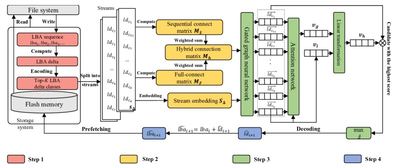
Figure 1: The workflow of the SGDP framework. In Step 1, we compress the search space and reduce the learning complexity. In Step 2, we compute the hybrid connection matrix $\textbf{M}_{h}$ with sequential and global information and embed the LBA delta stream into a matrix $\textbf{S}_{\Delta}$. In Step 3, using gated graph neural networks to update the latent node vectors. Each stream is represented as the combination of the local preference $\textbf{v}_{l}$ and global interaction $\textbf{v}_{g}$ by an attention network. In Step 4, we predict the candidate with the highest score and decode it to get the next accessed LBA for prefetching. This framework corresponds to the four steps of Algorithm 1.

Graph structures can effectively use nodes and edges to represent LBA (delta) and access sequence, and can mine intrinsic access patterns beyond chronological order in hybrid storage systems like relational databases. Therefore, to improve the performance of prefetching especially in applications with complex patterns, this work models the relations among LBA deltas using graph neural network, and proposes a novel method called Stream-Graph Neural Network-Based Data Prefetcher (SGDP), as shown in Figure 1. Specifically, we encode LBA deltas and split them into shorter streams. Then we build weighted directed graphs based on LBA delta streams and extract relations of sequential connection and temporal accesses of LBA deltas from each stream, which are represented as sequential connect matrices and full-connect matrices, respectively. By fusing those two matrices, we get hybrid matrices that contain the relations of LBA deltas. Finally, the hybrid matrix, along with embedding LBA deltas of each stream is fed into a gated graph neural network to learn access patterns for prefetching. Extensive experiments on eight real-world datasets show that SGDP outperforms the SOTA prefetchers in terms of performance and efficiency.

The contributions of this work are summarized as follows:

1. SGDP can accurately learn complex access patterns by capturing the relations of LBA deltas in each stream. The relations are represented by sequential connect matrices and full-connect matrices using graph structures.

2. To the best of our knowledge, SGDP is the first work that utilizes the stream-graph structure of the LBA delta in the data prefetching problem. Using gated graph neural networks and attention mechanisms, we extract and aggregate sequential and global information for better prefetching.

3. As a novel solution in the hybrid storage system, SGDP can be generalized to multiple variants by different stream construction methods, which further enhances its robustness and expands its application to various real-world scenarios.

4. SGDP outperforms SOTA prefetchers by 6.21% on hit ratio, 7.00% on effective prefetching ratio, and speeds up inference time by 3.13$\times$ on average. It has been verified in commercial hybrid storage systems in the experimental phase and will be deployed in the future product series.

II Related Work

Traditional Data Prefetcher The most commonly used prefetcher is the Stride prefetcher [27] which uses a reference prediction table to store the last few accessed LBAs and the stride to obtain the required LBA. Although it can capture a constant stride in sequential access patterns, it can hardly detect variable strides in irregular access patterns. Temporal prefetchers learn irregular access patterns by memorizing pairs of correlated LBAs [8, 34, 39, 40]. However, due to inconsistent correlation address pairs, these traditional methods cannot achieve good performance in practice.

Learning-based Data Prefetcher Prefetching needs to be accurate, as a small error in the numerical value of a prefetched LBA leads to useless prefetch and a waste of cache space and I/O bandwidth. Even though prefetching can be treated as a prediction problem, regression-based time-series prediction models like ARIMA are not widely considered by researchers. Classification-based methods seem more favoured because they can cover more LBA accesses, but not practical as it is hard to cover all LBAs. For example, in Microsoft Research Cambridge traces [2], the top-1000 most frequently occurring LBAs cover only 2.8% of all the LBA accesses, whereas the top-1000 most frequently occurring LBA deltas cover 91.7% of all LBA accesses [5]. To learn more complex access patterns, many deep learning approaches are proposed and consider the LBA delta as input directly [19]. DeepPrefetcher [20] transforms the LBA sequence into LBA deltas, then employs the word2vec model and LSTM architecture to capture the hidden feature in the input sequence. However, it is inefficient on large-scale trace datasets. Delta-LSTM is proposed [5] and addresses the large and sparse LBA space by co-learning top-$K$ LBA delta and I/O size features. Within top-$K$ (e.g., $K=1000$) classes, the searching space is restricted, which alleviates the class explosion problem. However, both of them do not consider the relations of LBA deltas to capture the more complex patterns (e.g., the continuous LBA accesses across many pages), which results in limited performance.

Prefetching with Graph-based Structure Complex patterns in LBA access streams can be constructed by graphs [43, 53]. Nexus uses metadata relationship graphs to assist prefetching decision-making [56]. Ainsworth et al. design a prefetcher for breadth-first searches on graphs [55]. These methods transform a sequence of observed LBAs into a directed graph, in which a node is utilized to represent a block access event to model block access patterns. However, LBA accesses are quite sparse, which results in large graphs in these LBA sequence-based methods and makes these prefetchers quite ineffective in practice.

III Preliminaries

Consider an LBA access sequence with length $n$:

$$\langle lba_{i}\rangle_{i=1}^{n}=\langle lba_{1},lba_{2},\ldots,lba_{n}\rangle,$$ (1)

in which $lba_{i}\in N$ represents the address number of the $i$-th accessed blocks. The data prefetching problem can be regarded as given $\langle lba_{i}\rangle_{i=1}^{n}$, predict $lba_{n+1}$. Following the previous learning-based prefetchers, we compute LBA deltas ($ld$):

$$ld_{i}=lba_{i+1}-lba_{i},$$ (2)

$$\langle ld_{i}\rangle_{i=1}^{n-1}=\langle ld_{1},ld_{2},\ldots,ld_{n-1}\rangle.$$ (3)

In order to get the prediction of the next LBA, $\widehat{lba}_{n+1}$, we predict the delta $\widehat{ld}_{n}$. Note that the variables with the $\hskip 2.84544pt\widehat{}\hskip 2.84544pt$ symbol denotes the predicted values. In short, the data prefetching problem is formulated as follows:

$$\widehat{lba}_{n+1}=lba_{n}+\widehat{ld}_{n}.$$ (4)

To restrict the model size, the number of classes of LBA deltas that needs to be predicted is capped to a fixed number of $K+1$. Here $K$ is acquired by top-$K$ most frequently occurring LBA delta in $\langle ld_{i}\rangle_{i=1}^{l-1}$, and the extra class is for the other infrequent LBA deltas. The prefetcher treats this extra class as no-prefetch because infrequent LBA delta is hard to predict. We redefine these $K+1$ classes as $LD=\{ld_{c_{0}},ld_{c_{1}},\ldots,ld_{c_{K+1}}\}$, $ld_{c_{0}}$ representing the no-prefetch class and $\{ld_{c_{1}},\ldots,ld_{c_{K+1}}\}$ representing the top-$K$ ones. The model predicts the $ld_{c_{i}}$ of the next LBA delta, and prefetches it when the predicted class is in the top-$K$ and does not prefetch if the class is $ld_{c_{0}}$. Using the LBA delta and Top-$K$ mechanism can effectively reduce the sparse problem and the search space of the model.

IV Methodology

IV-A LBA Delta Streams

It would yield expensive costs if building the directed graph of the LBA delta sequence generated by the whole LBA sequence (length $\geq 1\times 10^{7}$). To alleviate this problem, we use the concept of data access stream. We split the whole LBA delta sequence into shorter streams which represent the temporal access patterns. Specifically, we consider LBA accesses with close access times to be in the same stream. Whenever the time interval between two LBA accesses is longer than a preset time limit $T$ (e.g. $T=$ 0.1ms), the LBA sequence will be split to generate a new stream. We then split the LBA delta sequence correspondingly and use a sliding window inside each stream to generate equal-length LBA delta streams. A split LBA delta stream $\textbf{s}_{\Delta}$ can be represented by a vector $\textbf{s}_{\Delta}=[ld_{s,1},ld_{s,2},...,ld_{s,n}]$ in the chronological order, where $ld_{s,i}$ denotes the $i$-th LBA delta in the stream $\textbf{s}_{\Delta}$. The LBA delta stream is not only suitable for building directed graphs but also implies the temporal locality of LBA accesses.

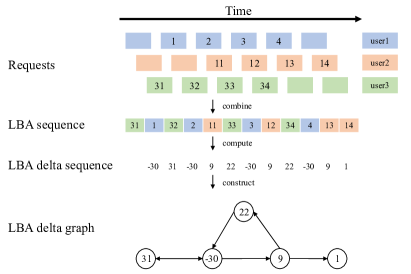
Figure 2: Example of LBA delta and graph.

IV-B LBA Delta Based Graph Structure

As discussed in Section II, LBA-based graph structure is ineffective for data prefetching in practice. To solve this problem, we propose a high-order graph based on the LBA delta. Here we present a toy example in Figure 2 to show that LBA deltas can also be represented by a directed graph. Consider three users sending concurrent sequential read requests. The concurrent requests are combined into one LBA sequence before being sent to the storage system. Following the LBA delta computation progress in Section IV-A, we can simplify the original LBA sequence that has 12 different LBAs and represent it with an LBA delta sequence with only 5 different nodes. We can build a directed graph based on the LBA delta sequence by using LBA deltas as a node and linking all the LBA deltas with their successor.

In contrast to previous works on extracting useful features from access patterns between nearby accessed LBAs only, we observed if an LBA request sequence is divided into several streams, different streams are possible to be accessed by a similar pattern. Non-sequential features can be extracted from the observed access patterns by monitoring the change (or difference) between successive LBA requests. This is achieved by learning the hybrid connection matrix (which contains adjacent and interactive relations) along with the embedded LBA deltas. Also, the number of the graph nodes is constant, that is $K+1$.

IV-C Weighted Directed Stream-based Graph

Without loss of generality, each LBA delta stream $\textbf{s}_{\Delta}$ can be modeled as a directed graph $\mathcal{G}_{\textbf{s}_{\Delta}}=(\mathcal{V}_{\textbf{s}_{\Delta}},\mathcal{E}_{\textbf{s}_{\Delta}})$. Each node in the directed graph $\mathcal{G}_{\textbf{s}_{\Delta}}$ expresses one of the classes of LBA deltas $ld_{s,a}\in LD$. We build the graph with two kinds of edges, as shown in Figure 3. The first one $(ld_{s,a},ld_{s,a+1})\in\mathcal{E}_{\textbf{s}_{\Delta}}$ represents the order in an LBA delta stream $\textbf{s}_{\Delta}$ by linking $ld_{s,a}$ to its successor $ld_{s,a+1}$. The second one $(ld_{s,a},ld_{s,b})\in\mathcal{E}_{\textbf{s}_{\Delta}}$ is built by fully connecting all nodes in the stream to capture the global information of each LBA delta stream. We denote the set of sequential edges as $\mathcal{E}^{S}_{\textbf{s}_{\Delta}}$ and full-connected edges as $\mathcal{E}^{F}_{\textbf{s}_{\Delta}}$. We compute the adjacency matrices $\mathbf{M}_{S}$ and $\mathbf{M}_{F}$ of $\mathcal{E}^{S}_{\textbf{s}_{\Delta}}$ and $\mathcal{E}^{F}_{\textbf{s}_{\Delta}}$ separately. As every LBA delta node might appear more than once in a stream, we normalize the weights on each edge in $\mathcal{E}_{\textbf{s}_{\Delta}}$. The weight of an edge is set to be its occurrence counts divided by the out-degree of its start node. The higher the weight, the stronger the correlation between the corresponding two nodes. The incoming parts of $\mathbf{M}_{S}$ and $\mathbf{M}_{F}$ are computed as Eq. (5) and (6),

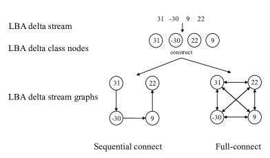
Figure 3: Example of two kinds of graphs.

$$\textbf{M}^{in}_{S}=\sum_{i=1}^{K+1}\frac{\textbf{1}((ld_{s,a},ld_{s,a+1})_{\mathcal{E}^{S}_{\textbf{s}_{\Delta}}})}{\textbf{1}((ld_{s,i},ld_{s,a+1})_{\mathcal{E}^{S}_{\textbf{s}_{\Delta}}})},\ (a\leq n-1),$$ (5)

$$\textbf{M}^{in}_{F}=\sum_{i=1}^{K+1}\frac{\textbf{1}((ld_{s,a},ld_{s,b})_{\mathcal{E}^{F}_{\textbf{s}_{\Delta}}})}{\textbf{1}((ld_{s,i},ld_{s,b})_{\mathcal{E}^{F}_{\textbf{s}_{\Delta}}})\times|b-a|},\ (a,b\leq n),$$ (6)

where $\textbf{1}(\cdot)$ is indicator function and the outgoing parts $\textbf{M}^{out}_{F}$ and $\textbf{M}^{out}_{F}$ is computed in the same manner. Then, we expand $\textbf{M}_{S}$ and $\textbf{M}_{F}$ to the same dimension, $\textbf{M}_{S},\textbf{M}_{F}\in\mathbb{R}^{(K+1)\times 2*(K+1)}$. To facilitate the fuse of information in $\textbf{M}_{S}$ and $\textbf{M}_{F}$, we conduct a weighted sum of them named as hybrid connection matrix $\textbf{M}_{h}$.

Then, the preprocessed LBA delta stream is embedded with the hybrid connection matrix $\textbf{M}_{h}$ and fed into a graph neural network. Specifically, we obtain each node vector $\overrightarrow{ld}_{s,i}\in\mathbb{R}^{d}$ that indicates the $d$-dimensional latent vector of the original $ld_{s,i}\in LD$. Each LBA delta stream $\textbf{s}_{\Delta}$ can be presented as an embedding matrix $\textbf{S}_{\Delta}$ by DeepWalk [58] where each node vector $\overrightarrow{ld}_{s,i}\in\mathbb{R}^{d}$ denotes a $d$-dimensional real-valued latent vector. Note that SGDP can support LBA streams of various lengths and various graph model constructing strategies.

IV-D Latent Node Vectors Updating

We apply the vanilla graph neural network (GNN) proposed by [49] and gated-recurrent-units-based GNN (gated GNN) [50] to obtain latent features of nodes. Specifically, for each LBA delta stream vector $\textbf{S}_{\Delta}=[\overrightarrow{ld}_{1}^{t-1},\overrightarrow{ld}_{2}^{t-1},...,\overrightarrow{ld}_{n}^{t-1}]$ in the graph $\mathcal{G}_{\textbf{s}_{\Delta}}$, the update functions can be formalized as,

$$\mathbf{a}^{t}=\mathbf{A}_{\textbf{M}_{h}}^{t-1}(\textbf{S}_{\Delta}\mathbf{W_{a}}^{t}+\mathbf{b_{a}}^{t}),$$ (7)

$$\mathbf{z}^{t}=\sigma(\mathbf{W_{z}}^{t}\mathbf{a}^{t}+\mathbf{U_{z}}^{t}\overrightarrow{ld}^{t-1}_{n}),$$ (8)

$$\mathbf{r}^{t}=\sigma(\mathbf{W_{r}}^{t}\mathbf{a}^{t}+\mathbf{U_{r}}^{t}\overrightarrow{ld}^{t-1}_{n}),$$ (9)

$$\tilde{\mathbf{h}}^{t}=tanh(\mathbf{W_{h}}^{t}\mathbf{a}^{t}+\mathbf{U_{h}}^{t}(\mathbf{r}^{t}\odot\overrightarrow{ld}^{t-1}_{n}),$$ (10)

$$\mathbf{h}^{t}=(1-\mathbf{z}^{t})\odot\overrightarrow{ld}^{t-1}_{n}+\mathbf{z}^{t}\odot\tilde{\mathbf{h}}^{t},$$ (11)

where $\mathbf{A}_{\textbf{M}_{h}}^{t-1}\in\mathbb{R}^{1\times 2n}$ is two rows of blocks (outgoing and incoming) in $\mathbf{M}_{h}$ corresponding to node $ld^{t-1}_{n}$. $\mathbf{a}^{t}$ extracts the contextual features of neighborhoods for node $ld^{t-1}_{n}$ with weight matrix $\mathbf{W_{a}}^{t}\in\mathbb{R}^{d\times 2d}$ and bias vector $\mathbf{b_{a}}^{t}\in\mathbb{R}^{2d}$. Then, we take $\mathbf{a}^{t}$ and previous LBA delta vector $\overrightarrow{lb}_{n}^{t-1}$ as input and feed them into the gated GNN. The updated functions are shown in Eq. (8)$\sim$(11). $\mathbf{z}^{t}$ and $\mathbf{r}^{t}$ are the updates and the reset gate, and control which features to be reserved or discarded. $\sigma(\cdot)$ represents the logistic sigmoid function and $\odot$ denotes the element-wise multiplication operator. $\mathbf{W_{z}}^{t}$, $\mathbf{W_{r}}^{t}$, $\mathbf{W_{h}}^{t}$ and $\mathbf{U_{z}}^{t}$, $\mathbf{U_{r}}^{t}$, $\mathbf{U_{h}}^{t}$ are the weight matrices to be learned. The final state $\mathbf{h}^{t}$ is the latent node vector, which is the sum of the candidate states and the previous hidden states. Note that the model will update all nodes until they converge.

IV-E Generating Stream Hybrid Embedding Vector

The next accessed LBA is strongly correlated with the previous ones, and that relationship is inversely proportional to the interval between the two LBAs. Therefore, we apply a hybrid embedding vector to extract features, i.e., local embedding and global embedding. Firstly, the local embedding vector named $\mathbf{v}_{l}^{t}$ is defined as the last accessed LBA delta $\overrightarrow{ld}_{n}^{t-1}$,

$$\mathbf{v}_{l}^{t}=\overrightarrow{ld}_{n}^{t-1}.$$ (12)

The global embedding vector $\mathbf{v}_{g}^{t}$ aggregates all node vectors in the LBA delta stream $\textbf{S}_{\Delta}$. Specially, we use the soft-attention approach to more effectively represent the different levels of priority, as Eq. (13) and (14) show,

$$\mathbf{\alpha}_{i}^{t}={\mathbf{q}^{t}}^{\top}\sigma(\mathbf{W_{1}}^{t}\overrightarrow{ld}_{n}^{t-1}+\mathbf{W_{2}}^{t}\overrightarrow{ld}_{i}^{t-1}+\mathbf{b}_{g}^{t}),$$ (13)

$$\mathbf{v}_{g}^{t}=\sum_{i=1}^{n}\mathbf{\alpha}_{i}^{t}\overrightarrow{ld}_{i}^{t-1},$$ (14)

where $\mathbf{W_{1}}^{t},\mathbf{W_{2}}^{t}\in\mathbb{R}^{d\times d}$ and $\mathbf{q}^{t}\in\mathbb{R}^{d}$ are weight matrices, and $\mathbf{b}_{g}^{t}\in\mathbb{R}^{d}$ is bias vector.

Finally, the hybrid embedding vector $\mathbf{v}_{h}^{t}$ combines the local embedding vector $\mathbf{v}_{l}^{t}$ and the global embedding vector $\mathbf{v}_{g}^{t}$ linearly, as the Eq. (15) shows,

$$\mathbf{v}_{h}^{t}=\mathbf{W_{f}}^{t}[\mathbf{v}_{l}^{t};\mathbf{v}_{g}^{t}]+\mathbf{b_{h}}^{t},$$ (15)

where $\mathbf{W_{f}}^{t}\in\mathbb{R}^{d\times 2d}$ is weight matrix and $\mathbf{b_{h}}^{t}\in\mathbb{R}^{d}$ is bias vector. The final hybrid embedding vector $\mathbf{v}_{h}^{t}$ of the LBA delta stream $\textbf{S}_{\Delta}$ is in the $d$ dimensions.

IV-F Forecasting and Prefetching

After extracting the hybrid embedding vector $\mathbf{v}_{h}^{t}$, we predict the score of each LBA delta candidate $\widehat{\mathbf{z}}_{i}^{t}$ in stream $\textbf{s}_{\Delta}$ by multiplying $\mathbf{v}_{h}^{t}$ and $\overrightarrow{ld}_{i}^{t-1}$ as

$$\widehat{\mathbf{z}}_{i}^{t}={\mathbf{v}_{h}^{t}}^{\top}\overrightarrow{ld}_{i}^{t-1}.$$ (16)

We take the candidate with the highest score as the predicted LBA delta. Besides, in order to train with labels, we need to compute the probability of each node $\widehat{\mathbf{y}}^{t}\in\mathbb{R}^{K+1}$ in the next step using the softmax function, which is

$$\widehat{\mathbf{y}}^{t}=\mathit{Softmax}(\widehat{\mathbf{z}}^{t}).$$ (17)

The loss function is the cross-entropy of prediction $\widehat{\mathbf{y}}^{t}$ and ground truth $\mathbf{y}^{t}$ with regularization, as shown in Eq. (18).

$$\mathcal{L}(\widehat{\mathbf{y}}^{t})=-\sum_{i=1}^{m}[\mathbf{y}_{i}^{t}\mathit{log}(\widehat{\mathbf{y}}_{i}^{t})+(1-\mathbf{y}_{i}^{t})\mathit{log}(1-\widehat{\mathbf{y}}_{i}^{t})]+\lambda\lVert\theta\rVert^{2}_{2},$$ (18)

where $\lambda$ is $\mathit{l2}$-norm penalty factor, $\theta$ is weight vectors.

Finally, we decode the index of $\max\widehat{\mathbf{z}}_{i}^{t}$ to $\widehat{ld}_{s,n+1}$, predict the next accessed LBA by Eq. (4), and prefetch the corresponding block from storage into the cache. Overall, we summarize the proposed SGDP framework in Algorithm 1.

Algorithm 1 The Workflow of SGDP Framework

Input: An LBA sequence $\langle lba_{i}\rangle_{i=1}^{l}=\langle lba_{1},lba_{2},\ldots,lba_{l}\rangle$ , the top number of most frequent LBA delta $K$, dimension of embedding vector of each LBA delta stream $d$, cache size $N$, maximum iteration $Q$, stop criteria $tol$.

1:  Step 1: LBA stream preprocessing

2:  Compute delta of each adjacent LBA pair in $\langle lba_{i}\rangle_{i=1}^{l}$ and get LBA delta $\langle ld_{i}\rangle_{i=1}^{l-1}=\langle ld_{1},ld_{2},\ldots,ld_{n-1}\rangle$.

3:  Encode $ld$s in all LBA streams by $top(K)$ to $LD$.

4:  Generate LBA delta stream $\textbf{s}_{\Delta}$ by time limit and slide window.

5:  Step 2: Embed LBA delta stream to a graph

6:  Compute $\textbf{M}_{S}$ by Eq. (5) and $\textbf{M}_{F}$ by Eq. (6).

7:  Expand $\textbf{M}_{S}$ and $\textbf{M}_{F}$ and conduct weighted sum to get $\textbf{M}_{h}$.

8:  Conduct embedding of each $\textbf{s}_{\Delta}\in\mathbb{R}^{n}$ into $\textbf{S}_{\Delta}\in\mathbb{R}^{d\times n}$.

9:  Step 3: Update hybrid embedding vector and training

10:  Initialize the parameters in the gated GNN model.

11:  for $q=1,...,Q$ do

12:     Compute the Eq.(7) $\sim$ Eq.(18) to fit each stream with the input $\textbf{M}_{h}$ and $\textbf{S}_{\Delta}$.

13:     Update the weight matrices list {$\mathbf{W_{z}}$, $\mathbf{W_{r}}$, $\mathbf{W_{h}}$, $\mathbf{U_{z}}$, $\mathbf{U_{r}}$, $\mathbf{U_{h}}$, $\mathbf{W_{1}}$, $\mathbf{W_{2}}$, $\mathbf{W_{f}}$} and vectors list {$\mathbf{b_{g}}$, $\mathbf{b_{h}}$} by Adam with ground truth y.

14:     Convergence checking: if $\mathcal{L}(\widehat{\mathbf{y}})<tol$, break; otherwise, continue.

15:  end for

16:  Step 4: Conduct forecasting and data prefetching

17:  Conduct Eq.(16) and get $\max\widehat{\textbf{z}}$ with the updated model.

18:  Decode it to $\widehat{ld}_{n}$ and conduct Eq.(4) to get $\widehat{lba}_{n+1}$.

19:  Read the corresponding block and prefetch it into the cache or conduct no prefetching.

Output: $\widehat{lba}_{n+1}$, blocks $\in\mathbb{R}^{N}$ in cache.

V Experimental Settings

V-A Datasets

We use representative eight datasets in production servers from different applications, including six datasets from an open-source benchmark MSRC and two datasets from a real enterprise storage system HW:

MSRC (Microsoft Research Cambridge) [2]: It collects a 1-week LBA sequence of live enterprise servers at Microsoft. We use its five datasets from different application scenes named {hm_1, mds_0, proj_0, prxy_0, src1_2}.

HW: It consists of three datasets collected from a real-world commercial hybrid storage system, which describes storage traffic characteristics on enterprise virtual desktop infrastructure and production servers. It intercepts the stream from an intra-enterprise storage system under different application scenarios and reads the storage system record logs directly. We named these three datasets as {hw_1, hw_2, hw_3}.

Table I provides the detail of the eight datasets from two data sources. Memory means the total amount of storage space that has been accessed in the trace. Sequential shows the percentage of sequential accesses in the trace.

TABLE I: Datasets Description

Source	Dataset	Length	Memory (GB)	Function	Sequential (%)
MSRC	hm_1	1.08$\times 10^{6}$	6.36	Hardware monitoring	39.9
	mds_0	4.23$\times 10^{5}$	8.48	Media server	65.2
	proj_0	1.17$\times 10^{6}$	4.056	Project directories	57.3
	prxy_0	4.03$\times 10^{5}$	5.18	Firewall/web proxy	37.6
	src1_2	1.15$\times 10^{6}$	2.0	Source control	58.5
HW	hw_1	1.39$\times 10^{6}$	930.29	hybrid storage system	55.8
	hw_2	2.58$\times 10^{5}$	600.46	hybrid storage system	95.1
	hw_3	1.73$\times 10^{5}$	902.22	hybrid storage system	43.7

V-B Compared Methods

We compare SGDP with the following methods from three categories: traditional prefetchers, regression-based prefetchers, and learning-based prefetchers.

No_pre means without any prefetching facilities and is used as a baseline to show the gain by other schemes.

Naïve Prefetcher treats the LBA stream as a whole sequence, i.e., $\widehat{ld}_{n}=ld_{n-1}$, and directly uses Eq. (4) to predict LBA.

Stride Prefetcher [6] simultaneously records 128 LBA access streams, and each of them tracks the last 3 LBA accesses. Each access is mapped to a stream based on hashing the most significant LBA. If the difference between the 3 LBA accesses matches, it will detect a stride and conduct a prediction.

ARIMA[9] treats the problem as a time-series prediction problem and applies the ARIMA model built from $t-\delta$ to $t$ to forecast the next LBA.

Informer [11] is the SOTA for time-series forecasting. Same as ARIMA, it takes the previous LBA delta sequence as input and predicts the following LBA.

DeepPrefetcher [20] captures the LBA delta patterns by employing the word2vec model and LSTM architecture for prefetching.

Delta-LSTM [5] is another learning-based prefetcher, which uses an LSTM-based model to predict the LBA delta for prefetching.

Besides, we set the sequences of LBA delta as the input for a fair comparison. There is a class explosion problem in DeepPrefetcher, which makes it unrealistic to train. To solve the problem, we restrict the top-$K$ class with $K=10000$. This $K=10000$ value is to balance the efficiency and accuracy based on our preliminary study. For Delta-LSTM and SGDP, we set top-$1000$ frequently occurring LBA deltas as input.

V-C Evaluation Criteria

HR@N (Hit Ratio) is the number of cache hits divided by the total number of memory requests over a given time interval. It is an important storage indicator given a fixed cache size $N$. That is,

$$\rm HR=\frac{\rm Cache\,\,Hits}{\rm Cache\,Hits+Cache\,\,Misses}\times 100\%.$$ (19)

EPR@N (Effective Prefetching Ratio) is the ratio of the number of correctly prefetched data to all executed prefetches given a fixed cache size $N$, which is strongly related to the prefetcher’s efficiency. That is,

$$\rm EPR=\frac{\rm Correct\,\,Prefetchings}{\rm All\,\,Prefetchings}\times 100\%.$$ (20)

Note that HR and EPR describe the prefetching results more precisely and feasible refer to Accuracy and Recall in DeepPrefetcher [20] and Delta-LSTM [5], respectively. We use HR and EPR in our work because they describe the prefetching results more precisely. Besides, there is a trade-off between HR and EPR in the subsection VI-B1 and some results are shown in Figure 4.

Besides, we feed the next step predicted LBA into the cache simulator based on the Least Recently Used (LRU) strategy for prefetching. LRU is a classical cache elimination algorithm. It selects the most recently unused LBA to retire.

V-D Implementation Details

We implemented SGDP for offline training and online testing by PyTorch [57]. All experiments are trained and tested on a computing server equipped with an Intel Xeon Platinum 8180M CPU@2.50GHz and an NVIDIA Tesla V100 GPU.

For a more fair and effective comparison, we normalize all LBA in increments of 8KB blocks and according to the I/O size of the 8KB block alignment and increment operations. We apply the 10-fold cross-validation method for training and testing, the same as SOTA methods. As for neural networks, all parameters are initialized with a Gaussian distribution with a means of 0 and a standard deviation of 0.1 with the latent vectors $d$ equaling 200 for all 8 datasets. Moreover, we set the initial learning rate to 1.5$\times 10^{-3}$ with decay by 95% after every 3 epochs, the batch size to 128 with 10 epochs, and the $\mathit{l2}$-norm penalty factor to 10^-5. Adam optimizer [12] with default parameter is applied for optimization. We set the stream split time interval $T$ as 0.1ms for HW and 0.01ms for MSRC, and set the top number of most frequent LBA delta $K$ as 1000 for SGDP. Note that since the preprocessed LBA stream is shorter, the training epoch can be smaller to prevent over-fitting, which is also useful to shorten the training time.

TABLE II: Single-step Results. The results are in percentage, the best results are in bold, the second ones are underlined, $N$ is the cache size.

Dataset	hw_1						hw_2						hw_3						hm_1
	HR@N			EPR@N			HR@N			EPR@N			HR@N			EPR@N			HR@N			EPR@N
	10	100	1000	10	100	1000	10	100	1000	10	100	1000	10	100	1000	10	100	1000	10	100	1000	10	100	1000
No_pre	0.0	0.3	54.2	0.0	0.0	0.0	1.0	1.1	1.1	0.0	0.0	0.0	0.0	0.1	1.3	0.0	0.0	0.0	2.7	25.3	98.3	0.0	0.0	0.0 [t]
Naïve	57.5	58.0	63.2	63.3	64.5	64.5	92.5	92.6	92.7	93.3	93.7	94.0	47.7	47.9	48.8	48.0	48.3	48.7	31.7	43.8	97.4	30.5	31.2	5.6
Stride	43.7	44.0	65.8	80.5	81.1	80.6	91.0	91.1	91.1	99.1	99.2	99.2	38.4	38.6	39.6	81.6	82.0	82.3	27.1	47.0	99.1	82.3	84.4	88.4
ARIMA	1.9	4.0	8.8	1.9	4.3	6.2	82.8	82.9	83.0	85.9	86.2	86.4	0.3	0.3	1.3	0.2	0.3	0.3	3.5	19.0	95.2	2.7	5.2	2.5
Informer	0.2	0.9	5.8	0.3	0.9	2.9	1.0	1.1	1.1	0.0	0.0	0.0	0.0	0.0	0.9	0.0	0.0	0.0	1.1	14.0	90.4	0.1	0.7	0.7
DeepPrefetcher	74.3	74.6	79.2	75.4	75.9	76.5	92.2	92.5	92.8	93.4	94.0	94.5	50.4	50.7	51.7	50.4	50.7	51.2	38.5	59.1	99.3	38.5	56.0	46.1
Delta-LSTM	74.4	74.8	79.3	75.5	76.0	76.6	92.5	92.8	93.1	93.7	94.2	94.7	56.4	56.8	57.9	66.2	66.8	67.2	30.0	50.6	99.3	57.7	72.8	87.6 [b]
SGDP	79.2	79.5	85.8	82.9	83.5	81.6	93.0	93.0	93.1	97.5	97.7	97.8	76.0	76.6	77.5	88.9	89.5	90.1	38.1	55.7	99.4	87.8	90.1	86.2 [t]
SGDPl	78.5	78.8	84.9	82.1	82.7	80.6	92.9	93.1	93.2	97.0	97.2	97.4	78.5	79.0	79.8	83.6	84.2	84.7	43.1	61.4	99.1	46.3	60.8	24.4
SGDPp	75.7	78.2	83.6	77.6	80.4	79.6	93.7	94.0	94.2	94.4	95.0	95.4	48.1	48.3	49.6	72.1	73.1	75.1	43.9	62.9	99.4	46.8	63.8	34.8 [b]
Dataset	mds_0						proj_0						prxy_0						src1_2
	HR@N			EPR@N			HR@N			EPR@N			HR@N			EPR@N			HR@N			EPR@N
	10	100	1000	10	100	1000	10	100	1000	10	100	1000	10	100	1000	10	100	1000	10	100	1000	10	100	1000
No_pre	13.2	35.0	61.0	0.0	0.0	0.0	6.1	28.7	35.2	0.0	0.0	0.0	20.1	40.7	48.8	0.0	0.0	0.0	3.9	34.8	48.2	0.0	0.0	0.0 [t]
Naïve	54.3	68.2	85.2	47.8	51.1	52.2	61.1	70.1	74.3	58.7	59.7	60.8	46.4	64.3	72.7	35.1	38.5	40.9	60.5	73.0	80.8	59.9	63.1	66.3
Stride	47.3	62.2	79.8	82.3	90.6	89.8	51.0	61.1	65.4	82.5	88.1	88.3	40.3	56.5	63.8	69.6	81.1	81.4	48.3	63.8	73.4	81.0	89.6	92.0
ARIMA	16.6	37.4	58.3	8.6	9.2	12.0	12.9	33.5	39.3	12.0	10.1	10.4	19.9	42.2	52.3	6.5	7.2	8.2	14.6	42.0	54.8	19.5	17.7	19.2
Informer	9.6	28.3	54.5	0.3	1.2	5.2	3.9	19.8	34.7	0.1	0.5	2.3	13.7	32.1	46.9	0.0	0.0	0.2	1.7	22.5	45.3	0.0	0.1	0.6
DeepPrefetcher	60.7	73.7	88.5	66.9	77.5	83.3	72.6	79.1	82.8	75.0	78.6	81.5	57.0	70.2	77.4	63.5	70.4	73.9	74.5	82.9	89.0	76.2	80.9	87.0
Delta-LSTM	57.3	69.6	86.2	80.2	87.8	89.8	62.3	69.1	73.3	84.3	86.2	87.4	52.2	64.2	71.3	75.7	79.3	80.9	70.0	79.6	86.2	77.5	81.3	87.2 [b]
SGDP	66.0	76.3	91.6	80.2	87.0	88.4	73.4	78.5	82.1	84.0	87.6	88.2	62.2	73.2	79.9	76.3	83.3	84.1	75.4	83.1	88.8	82.5	88.5	90.8 [t]
SGDPl	66.1	77.5	92.1	65.4	73.9	79.6	75.5	81.1	84.6	79.8	83.6	85.6	64.1	76.5	83.0	65.7	74.3	78.4	76.3	83.9	89.4	81.5	87.4	89.3
SGDPp	67.4	79.8	92.6	68.7	81.9	87.9	73.7	81.3	85.2	74.5	80.2	83.9	63.9	76.2	83.0	64.9	72.6	76.1	74.9	84.8	89.8	76.1	84.0	87.3 [b]

TABLE III: Average Results of Multi-step Prefetching. The results are in percentage, the best results are in bold, and the cache size is 100.

Metric	HR@100										EPR@100
	1	2	3	4	5	6	7	8	9	10	1	2	3	4	5	6	7	8	9	10
DeepPrefetcher	74.0	76.1	76.7	77.1	77.2	77.1	77.1	77.0	77.0	76.9	73.1	60.7	52.5	46.5	42.0	38.3	35.3	32.8	30.7	28.8 [t]
Delta-LSTM	70.2	74.9	77.1	78.0	78.5	78.9	79.3	79.6	79.8	80.0	81.5	72.3	65.9	60.6	56.3	52.6	49.5	46.8	44.5	42.3 [b]
SGDP	77.0	78.3	78.9	79.3	79.6	79.8	80.0	80.1	80.3	80.3	88.4	80.5	74.0	68.9	64.6	60.9	57.7	54.9	52.7	50.5 [t]
SGDPl	78.9	80.7	81.4	81.8	82.2	82.4	82.5	82.6	82.7	82.7	80.5	70.2	62.9	57.5	53.1	49.6	46.6	44.0	41.8	39.8
SGDPp	75.7	77.4	78.1	78.6	78.9	79.1	79.2	79.3	79.5	79.5	78.9	68.3	60.8	55.1	50.6	46.8	43.7	41.1	38.8	36.7

VI Experimental Results

VI-A Results of Single-Step Prefetching

We analyze the results of data prefetching conducted by SGDP and the compared methods on different datasets in the case of single-step Prefetching, as reported in Table II. The detailed analysis is presented in the following.

ARIMA and Informer Time-series forecasting models (ARIMA and Informer) perform the worst, excepting the case of hw_2 trace where ARIMA achieves around 80% HR as this dataset has a very high degree of sequential access (95.1%). ARIMA and Informer take LBA delta inputs as scalar variables and can produce a correct prediction if the input sequences are steady. As there are frequent large fluctuations in complex non-sequential access patterns, ARIMA and Informer prompt incorrect LBA access. The worst results shown in almost all cases confirm our claims that regression-based approaches are not feasible for accurate and complex data prefetching.

Naïve and Stride Prefetcher Traditional prefetchers (Naïve and Stride) have relatively stable performances in sequential access. However, for the random accesses, those traditional prefetchers encounter a big gap compared to SGDP. Moreover, Stride always achieves higher EPR while lower HR as it is more laziness and only prefetches when detecting an inside-page stride. As a result, it prefetches less and has higher accuracy for sequential access. In other words, although Stride has a high EPR, it prefetches less and gets quite low HR, which makes it impractical. Overall, the robustness performance of the Naïve and Stride Prefetcher is poor, especially for completely random access.

Delta-LSTM, DeepPrefetcher and SGDP Learning-based prefetchers (Delta-LSTM, DeepPrefetcher and SGDP) cover all highest HR and almost the highest EPR. SGDP has higher HR than DeepPrefetcher/Delta-LSTM in 19/24 out of all 24 cases, and 24/19 about EPR. Specifically, Delta-LSTM and DeepPrefetcher share a similar structure and show a similar effect. DeepPrefetcher has a larger LBA delta candidates pool which leads to more prefetching and lowers accuracy, reflected in lower average EPR (71.6% compared to 80.3%). On the contrary, Delta-LSTM prefetches more accurately but with fewer blocks, which leads to lower HR (70.8% compared to 73.5%). To be fair, as SGDP takes the top-1000 LBA delta as input (same as Delta-LSTM), the comparison to Delta-LSTM can prove that SGDP has better feature extraction ability.

VI-B Ablation study and SGDP Variants by Stream Construction

VI-B1 Retaining top-$K$ delta value (SGDP_l)

SGDP considers the top-1000 most frequently occurring LBA delta in the whole search space. Considering more LBA delta values further increases the model coverage, but also increases the search space and degrades the accuracy of the model. So to explore it quantitatively and prove the HR-EPR trade-off, we apply the top-10000 LBA delta for model building and name it SGDP_large, or SGDP_l for brevity.

The experiment of SGDP_l confirms the trade-off of HR-EPR. As Table II shows, SGDP_l achieves 1.5% slightly higher than SGDP in terms of HR while showing a large gap with 9.6% loss than SGDP in terms of EPR. Compared to DeepPrefetcher, which also uses top-10000 LBA delta as input, SGDP_l maintains higher HR in 23 cases and higher EPR in 20 cases. Notice that for dataset hm_1, SGDP_l gets a low EPR@1000 (24.4%). The reason is that with an extremely high HR@1000 (99.4%, almost all hit), SGDP_l prefetches extra useless blocks without harm to HR, leading to an obvious decline of EPR.

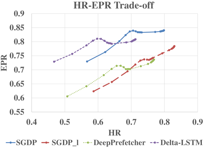
Figure 4: HR-EPR trade-off.

To further verify the effectiveness of SGDP and the HR-EPR trade-off, we conduct extra tests on dataset prxy_0 by testing Delta-LSTM, DeepPrefetcher, SGDP and SGDP_l on 20 different cache sizes ({5, 10, 20, $\cdots$ ,90 and 100, 200, $\cdots$, 900, 1000}). As shown in Figure 4, the top-10000 methods (SGDP_l and DeepPrefetcher) show higher HR but lower EPR than their top-1000 counterparts (SGDP and Delta-LSTM). The two pairs of top-$K$ comparisons confirm that SGDPs achieve better performance consistently than other methods.

VI-B2 Stream partition with page (SGDP_p)

Considering the spatially localized relevance of LBA access patterns, we divide the entire search space by 64MB size page, record the LBA access streams on each page simultaneously, and perform parallel prediction in each page stream for prefetching the next block inside the page stream. We call it SGDP_p. SGDP_p models LBA deltas, as 64MB page contains 8192 unique blocks, the total LBA delta candidate class of SGDP_p is 16383 ($\pm 8191$) instead of top-$K$ classes.

SGDP_p keeps the best HR results on half of all cases. Its average HR is slightly lower than SGDP and SGDP_l, but still higher than other methods. HR of SGDP_p on hw_3 encounters a severe drop. The reason is that hw_3 is the shortest and has the second-largest storage capacity, which means the LBAs are much more sparse. SGDP_p needs at least an LBA stream with length 2 to generate an LBA delta stream. But as hw_3 cross over $1.4\times 10^{4}$ pages, the average length of inside-page-stream is 12.4, which means SGDP could not perform prefetching on 1/12 of data points. Nevertheless, SGDP_p obtains the highest HR (79.9%) on all datasets except hw_3 on average. Therefore, it could be concluded that SGDP_p performs well in real-world scenarios with sufficient data.

VI-C Multi-step Prefetching

We further evaluate the performance of SGDP methods in multi-step prefetching based on rolling prediction. We feed the prediction of LBA back to the aforementioned learning-based prefetchers and get the rolling prediction for the next LBAs. The experiments are performed on cache size 100 with a rolling step from 2 to 10. The average results of HR@100 and EPR@100 are reported in Table LABEL:roll_results. Overall, SGDP_l has the best HR@100 on all steps on average, and SGDP achieves the best EPR@100. SGDP_p shows worse results than SGDP and SGDP_l. SGDP_p gets the highest HR@100 (from 79.6% to 83.8%) on average in all steps on all the datasets except hw_3 as it is too sparse. The second best method is SGDP_l, of which HR@100s range from 78.9% to 83.0%. These results demonstrate that SGDP methods are able to keep their superiority and robustness in multi-step prefetching.

TABLE IV: The number of predictions inferred per second by learning-based methods.

	hw_1	hw_2	hw_3	hm_1	mds_0	proj_0	prxy_0	src1_2	avg
Delta-LSTM	89.4	87.4	94.5	92.4	90.7	91.5	88.4	95.1	91.2
DeepPrefetcher	208.2	154.5	194.2	160.1	248.4	178.4	187.9	249.6	197.7
SGDP	644.5	692.4	666.1	515.2	543.5	553.3	470.0	550.7	579.5
SGDPl	634.7	686.9	614.7	500.1	651.4	663.9	526.3	670.7	618.6
SGDPp	599.5	645.6	593.9	567.0	491.7	529.3	574.8	558.7	570.1

VI-D Offline Training and Online Testing Efficiency

The offline training time in dataset hw_1 for SGDPs is 0.37 hours, and the training time for other learning-based methods is about 1.1 hours. The GPU utilization is 24%, the parameter number is 192,500, and the flop number is 48,570,779. For the online inference test, the GPU utilization is 10%, the model size is 1.47 MB, and the flop number is 1,884,055. Furthermore, to verify the practicality of SGDP compared to the other methods, we collect statistics of inference time as shown in Table VI. SGDPs process 469 to 670 LBA deltas per second, while Delta-LSTM and DeepPrefetcher can only process 91.2 and 197.7 on average. SGDP_l speeds up inference time up to 3.13$\times$ than DeepPrefetcher. Overall, SGDPs show much higher efficiency and practicality for real deployment applications.

VII Conclusions

To improve the performance of the data prefetcher in practice, this paper proposed SGDP, a novel stream-graph-based data prefetcher. SGDP takes each LBA delta stream as a weighted directed graph fusing both sequential and global features. By gated GNN and attention mechanism, SGDP extracts and aggregates the sequential and global information for better data prefetching. The experiment results from eight different real-world datasets demonstrate that SGDP outperforms SOTA methods and high speeds up inference time. The generalized SGDP variants can further adapt to extensive application scenarios. This novel data prefetcher has been verified in commercial hybrid storage systems in the experimental phase and will be deployed in the future product series.

Appendix A: All Results of Rolling Prediction Based Multi-Step Prefetching

We summarize the detailed results of multi-step prefetching in Table V. As reported in the Table V, SGDP and its variants achieve the best results in 80 cases and 52 cases in terms of HR@100 and EPR@100, respectively. We also visualize the results of the averaged results of all datasets and two representative datasets as shown in Fig. 5. On hw_1 dataset, SGDP stably performs the best with both the highest HR@100 and EPR@100. On src1_2, SGDP_p maintains highest HR@100 while SGDP have highest EPR@100.

Appendix B: Inference Efficiency

To verify the practicality of SGDP compared to the SOTA methods, we collect statistics of inference time and report the detailed results of the number of LBA delta predictions that can be inferred per second by learning-based methods in Table VI. SGDP and its variants process 469 to 670 LBA deltas per second, while Delta-LSTM and DeepPrefetcher are only able to process 91.2 and 197.7 on average respectively. SGDP_l speed up inference time up to 3.13 times than DeepPrefetcher. Overall, SGDP and its variants show much higher efficiency and practicality.

Appendix C: All Results of Single-step Prefetching Based on Different Cache Sizes

We summarize the results of single-step prefetching about all eight datasets based on 20 different cache sizes ($\{5,10,20,\cdots,90,100,200,\cdots,900,1000\}$) from Table VII to TableXIV. As reported in the Tables, SGDP and its variants (SGDP_l and SGDP_p) achieve the best results in all 160 cases and 83 cases in terms of HR and EPR, respectively. As for EPR, our models are not far from the maximum (mostly within 1%) in the non-first case.

Appendix D: Results and Algorithm Reproducing

In data prefetch, researchers rarely open-source their code. We have contacted most authors for their baseline codes and benchmarks, but the response is almost non-existent, which makes it difficult for us to compare baselines. We could not find the related source code for graph-based methods. However, we can guarantee that the two learning-based methods we compared are the best methods available. They achieve better results than all graph-based ones using the same datasets, so we choose them as the baselines. Although the authors of the two methods did not give us the code directly, we received confirmation and positive feedback from them on our reproduction. So, we are confident that our results are now SOTA and definitely better than all the previous graph-based methods.

As for the discussed time-series-based methods in our paper, i.e., ARIMA and Informer, they are often discussed as baselines described in our Related Work section, it is reasonable to use ARIMA and Informer as baselines. As the other researchers said in their paper, those time-series-based methods perform well in datasets which have more sequence access patterns.

Researchers in this field hardly fully open-source their code, which not only makes it difficult for us to reproduce their methods but also hinders the development of the field. Therefore, we sincerely hope to promote the openness and development of the storage field and help more developers and researchers enter the community more efficiently by making our source code, datasets, and our reproduced and validated baselines available.

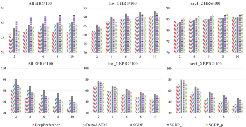
Figure 5: Visualized Results of Multi-step Prefetching

TABLE V: Results of Multi-step Prefetching. The results are in percentage, and the best results are highlighted in bold.

	Metrics	HR@100										EPR@100
Dataset		1	2	3	4	5	6	7	8	9	10	1	2	3	4	5	6	7	8	9	10
hw_1	DeepPrefetcher	74.6	82.2	85.3	87.4	88.4	89.1	89.7	90.1	90.2	90.3	75.9	68.2	63.0	59.2	55.8	52.8	50.3	48.0	45.8	43.9 [t]
	Delta-LSTM	74.8	82.3	85.4	87.6	88.6	89.2	89.9	90.3	90.4	90.5	76.0	68.4	63.2	59.5	56.1	53.2	50.6	48.4	46.2	44.3 [b]
	SGDP	79.5	85.7	88.3	90.2	91.2	91.9	92.5	92.9	93.2	93.4	83.5	77.1	72.4	68.8	65.5	62.6	60.1	57.8	55.6	53.6 [t]
	SGDPl	78.8	84.7	87.1	88.8	89.9	90.8	91.3	91.8	92.1	92.3	82.7	76.1	71.0	67.1	63.7	60.8	58.1	55.8	53.6	51.5
	SGDPp	78.2	83.8	86.0	87.4	88.3	88.9	89.5	89.9	90.1	90.1	80.4	73.6	68.1	64.0	60.5	57.4	54.7	52.1	49.6	47.3 [b]
hw_2	DeepPrefetcher	92.5	93.4	93.7	93.9	94.0	94.1	94.1	94.1	94.2	94.2	94.0	89.6	85.7	82.2	79.0	76.0	73.3	70.7	68.3	66.0 [t]
	Delta-LSTM	92.8	93.6	94.0	94.3	94.4	94.5	94.5	94.6	94.6	94.6	94.2	89.9	86.2	83.0	80.0	77.2	74.7	72.4	70.2	68.1 [b]
	SGDP	93.0	94.1	94.5	94.8	94.9	95.0	95.1	95.1	95.2	95.2	97.7	96.0	94.7	93.4	92.3	91.3	90.4	89.4	88.5	87.7 [t]
	SGDPl	93.1	94.1	94.6	94.8	95.0	95.1	95.2	95.2	95.3	95.3	97.2	95.2	93.3	91.7	90.1	88.7	87.3	85.9	84.6	83.4
	SGDPp	94.0	95.1	95.5	95.7	95.9	96.0	96.0	96.0	96.1	96.1	95.0	91.2	88.0	85.0	82.3	79.7	77.4	75.0	72.9	70.8 [b]
hw_3	DeepPrefetcher	50.7	51.8	51.8	51.8	51.8	51.8	51.8	51.8	51.8	51.8	50.7	34.9	26.3	21.1	17.7	15.2	13.3	11.8	10.6	9.7 [t]
	Delta-LSTM	56.8	60.7	67.8	68.3	68.4	68.5	68.4	68.4	68.4	68.4	66.8	52.4	46.9	41.1	36.5	32.8	29.7	27.1	25.3	23.5 [b]
	SGDP	76.6	77.7	78.0	78.0	78.0	78.0	78.0	78.0	78.1	78.0	89.5	81.6	74.4	68.9	63.8	59.9	56.1	53.1	50.8	48.2 [t]
	SGDPl	79.0	80.2	80.5	80.6	80.8	80.8	80.8	80.8	80.9	80.8	84.2	73.8	65.3	58.9	53.5	49.2	45.3	42.2	39.5	37.0
	SGDPp	48.3	48.5	48.5	48.6	48.6	48.7	48.7	48.9	49.2	49.3	73.1	61.6	53.4	47.5	42.9	39.2	36.2	34.1	32.8	31.5 [b]
hm_1	DeepPrefetcher	59.1	60.0	59.2	58.2	57.1	56.1	55.2	54.4	53.6	53.0	56.0	39.6	29.8	23.5	19.1	16.0	13.7	11.9	10.5	9.4 [t]
	Delta-LSTM	50.6	55.5	56.7	57.8	58.7	59.3	59.9	60.2	60.4	60.6	72.8	63.5	54.9	48.6	43.6	39.6	36.3	33.5	31.5	29.5 [b]
	SGDP	55.7	55.8	55.5	55.3	55.1	54.9	54.6	54.3	54.1	54.0	90.1	80.5	72.0	64.9	59.2	54.2	50.0	46.6	44.8	42.3 [t]
	SGDPl	61.4	63.1	63.6	63.7	63.4	63.1	62.8	62.4	62.1	61.8	60.8	45.1	35.8	29.7	25.2	21.9	19.3	17.2	15.5	14.1
	SGDPp	62.9	65.0	65.7	65.8	65.8	65.4	65.1	64.8	64.5	64.1	63.8	48.6	39.2	32.7	28.0	24.3	21.5	19.2	17.4	15.8 [b]
mds_0	DeepPrefetcher	73.7	81.3	81.7	81.8	81.6	81.2	80.9	80.6	80.3	79.9	77.5	61.3	50.5	42.6	36.3	31.2	27.4	24.4	21.9	19.9 [t]
	Delta-LSTM	69.6	75.6	77.2	78.2	79.0	79.7	80.3	80.9	81.4	81.8	87.8	80.7	74.6	69.4	65.2	61.4	58.1	55.2	52.7	50.4 [b]
	SGDP	76.3	76.9	77.4	77.8	78.1	78.5	78.9	79.1	79.4	79.5	87.0	78.1	71.1	65.4	60.7	56.6	53.2	50.3	47.7	45.3 [t]
	SGDPl	77.5	78.9	79.5	79.8	80.0	80.1	80.2	80.3	80.3	80.3	73.9	59.7	49.8	43.0	37.8	33.6	30.4	27.8	25.5	23.5
	SGDPp	79.8	82.0	82.9	83.6	84.0	84.3	84.6	84.8	85.0	85.0	81.9	71.3	63.2	56.9	51.5	47.1	43.3	40.2	37.3	34.7 [b]
proj_0	DeepPrefetcher	79.1	81.3	81.7	82.0	82.2	82.2	82.3	82.2	82.3	82.2	78.6	64.6	55.1	47.9	42.4	37.8	34.2	31.1	28.5	26.4 [t]
	Delta-LSTM	69.1	76.9	78.4	79.1	79.5	79.9	80.2	80.5	80.7	80.9	86.2	79.6	72.7	67.1	62.3	58.2	54.6	51.5	48.8	46.3 [b]
	SGDP	78.5	78.9	79.1	79.3	79.5	79.7	79.8	79.9	80.1	80.1	87.6	78.2	70.7	64.5	59.5	55.1	51.4	48.1	45.4	42.9 [t]
	SGDPl	81.1	81.9	82.3	82.6	82.9	83.1	83.2	83.3	83.5	83.5	83.6	72.4	64.0	57.4	52.1	47.8	44.1	41.0	38.3	36.0
	SGDPp	81.3	82.1	82.4	82.7	82.9	83.1	83.1	83.3	83.5	83.5	80.2	67.7	58.7	51.9	46.5	42.1	38.5	35.5	32.9	30.6 [b]
prxy_0	DeepPrefetcher	70.2	75.0	76.2	76.8	77.2	77.5	77.6	77.5	77.6	77.6	70.4	58.4	49.3	42.6	37.5	33.5	30.1	27.3	25.0	23.1 [t]
	Delta-LSTM	64.2	71.5	73.2	74.1	74.8	75.4	76.1	76.4	76.7	77.0	79.3	72.8	65.6	59.9	55.4	51.4	48.3	45.3	42.9	40.7 [b]
	SGDP	73.2	73.9	74.4	74.6	75.3	75.5	75.6	75.7	76.1	76.1	83.3	72.3	64.3	58.0	53.2	49.0	45.5	42.5	40.1	37.6 [t]
	SGDPl	76.5	77.7	78.3	78.7	79.4	79.6	79.8	79.9	80.2	80.2	74.3	61.4	53.1	47.0	42.5	38.6	35.5	32.8	30.7	28.6
	SGDPp	76.2	77.2	77.8	78.2	79.0	79.3	79.6	79.8	80.1	80.1	72.6	59.1	50.4	44.0	39.5	35.8	32.7	30.1	28.0	26.0 [b]
src1_2	DeepPrefetcher	82.9	84.1	84.5	84.8	85.0	85.2	85.5	85.6	85.9	86.0	80.9	68.9	60.0	53.3	48.0	43.7	40.1	37.1	34.5	32.3 [t]
	Delta-LSTM	79.6	83.3	84.0	84.4	84.7	85.1	85.4	85.7	85.9	86.0	81.3	71.3	63.0	56.4	51.3	47.2	43.7	40.7	38.1	35.9 [b]
	SGDP	83.1	83.7	84.1	84.5	84.8	85.0	85.4	85.5	85.8	85.9	88.5	79.8	72.8	67.1	62.4	58.3	54.9	51.7	49.0	46.5 [t]
	SGDPl	83.9	84.8	85.3	85.7	86.0	86.3	86.7	86.8	87.1	87.2	87.4	78.3	71.0	65.1	60.4	56.3	52.8	49.7	47.0	44.5
	SGDPp	84.8	85.7	86.0	86.3	86.6	86.8	87.0	87.3	87.5	87.5	84.0	73.4	65.2	58.7	53.6	49.2	45.5	42.3	39.5	37.0 [b]

TABLE VI: The number of LBA delta predictions that can be inferred per second by learning-based methods.

	hw_1	hw_2	hw_3	hm_1	mds_0	proj_0	prxy_0	src1_2	avg
Delta-LSTM	89.4	87.4	94.5	92.4	90.7	91.5	88.4	95.1	91.2
DeepPrefetcher	208.2	154.5	194.2	160.1	248.4	178.4	187.9	249.6	197.7
SGDP	644.5	692.4	666.1	515.2	543.5	553.3	470.0	550.7	579.5
SGDPl	634.7	686.9	614.7	500.1	651.4	663.9	526.3	670.7	618.6
SGDPp	599.5	645.6	593.9	567.0	491.7	529.3	574.8	558.7	570.1

TABLE VII: Results of single-step prefetching based on different cache sizes about dataset hw_1.

HR@N
	5	10	20	30	40	50	60	70	80	90	100	200	300	400	500	600	700	800	900	1000
No_pre	0	0	0	0	0	0	0	0.3	0.3	0.3	0.3	0.4	1.7	2.6	2.7	3.1	7.6	15.6	38.9	54.2
Naive	56.9	57.5	57.8	57.9	57.9	57.9	57.9	57.9	58.0	58.0	58.0	58.1	58.2	58.9	59.2	59.5	59.7	59.9	61.6	63.2
Stride	43.6	43.7	43.8	43.9	43.9	43.9	43.9	44.0	44.0	44.0	44.0	44.0	44.6	45.4	45.7	46.0	46.2	50.2	53.8	65.8
ARIMA	1.5	1.9	2.3	2.6	3.0	3.1	3.1	3.4	3.8	3.9	4.0	4.3	4.5	5.0	6.0	6.7	7.6	8.0	8.3	8.8
Informer	0.2	0.2	0.4	0.5	0.5	0.6	0.7	0.7	0.8	0.8	0.9	1.3	1.6	2.0	2.4	3.9	4.4	5.2	5.5	5.8
DeepPrefetcher	73.9	74.3	74.5	74.6	74.6	74.6	74.6	74.6	74.6	74.6	74.6	74.7	74.8	75.3	75.7	75.7	75.9	76.5	77.8	79.2
Delta-LSTM	74.0	74.4	74.6	74.7	74.7	74.7	74.7	74.7	74.8	74.8	74.8	74.8	74.9	75.4	75.8	75.8	76.0	76.6	77.9	79.3
SGDP	78.7	79.2	79.4	79.4	79.4	79.5	79.5	79.5	79.5	79.5	79.5	79.5	79.6	79.9	80.2	80.3	80.4	81.3	82.4	85.8
SGDPl	77.9	78.5	78.7	78.8	78.8	78.8	78.8	78.8	78.8	78.8	78.8	78.9	79.0	79.3	79.6	79.6	79.8	80.7	81.7	84.9
SGDPp	74.9	75.7	76.7	77.1	77.4	77.6	77.7	77.9	78.0	78.1	78.2	78.5	78.6	79.0	79.3	79.4	79.5	80.2	81.1	83.6
EPR@N
	5	10	20	30	40	50	60	70	80	90	100	200	300	400	500	600	700	800	900	1000
Naive	61.1	63.3	64.3	64.4	64.4	64.4	64.5	64.5	64.5	64.5	64.5	64.6	64.8	64.9	65.0	65.1	65.1	65.2	64.7	64.5
Stride	80.2	80.5	81.0	81.0	81.0	81.1	81.1	81.1	81.1	81.1	81.1	81.1	81.2	81.3	81.4	81.4	81.5	81.3	81.1	80.6
ARIMA	1.5	1.9	2.5	2.8	3.2	3.3	3.3	3.6	4.1	4.2	4.3	4.4	4.7	5.1	5.3	5.6	5.7	6.0	6.2	6.2
Informer	0.2	0.3	0.4	0.5	0.6	0.6	0.7	0.7	0.8	0.8	0.9	1.1	1.4	1.7	2.1	2.3	2.6	2.8	2.8	2.9
DeepPrefetcher	74.6	75.4	75.8	75.8	75.8	75.8	75.9	75.9	75.9	75.9	75.9	75.9	76.0	76.2	76.4	76.5	76.5	76.5	76.5	76.5
Delta-LSTM	74.7	75.5	75.9	75.9	75.9	76.0	76.0	76.0	76.0	76.0	76.0	76.0	76.1	76.3	76.5	76.6	76.6	76.6	76.6	76.6
SGDP	81.9	82.9	83.4	83.4	83.4	83.5	83.5	83.5	83.5	83.5	83.5	83.5	83.6	83.6	83.7	83.7	83.7	83.4	83.0	81.6
SGDPl	80.9	82.1	82.6	82.6	82.6	82.7	82.7	82.7	82.7	82.7	82.7	82.8	82.9	82.9	83.0	83.0	83.1	82.7	82.3	80.6
SGDPp	76.4	77.6	78.8	79.2	79.6	79.8	80.0	80.1	80.2	80.3	80.4	80.8	80.9	81.0	81.1	81.2	81.2	80.9	80.7	79.6

TABLE VIII: Results of single-step prefetching based on different cache sizes about dataset hw_2.

HR@N
	5	10	20	30	40	50	60	70	80	90	100	200	300	400	500	600	700	800	900	1000
No_pre	1.0	1.0	1.0	1.1	1.1	1.1	1.1	1.1	1.1	1.1	1.1	1.1	1.1	1.1	1.1	1.1	1.1	1.1	1.1	1.1
Naive	92.3	92.5	92.5	92.5	92.6	92.6	92.6	92.6	92.6	92.6	92.6	92.7	92.7	92.7	92.7	92.7	92.7	92.7	92.7	92.7
Stride	91.0	91.0	91.0	91.0	91.1	91.1	91.1	91.1	91.1	91.1	91.1	91.1	91.1	91.1	91.1	91.1	91.1	91.1	91.1	91.1
ARIMA	82.6	82.8	82.8	82.8	82.8	82.9	82.9	82.9	82.9	82.9	82.9	82.9	83.0	83.0	83.0	83.0	83.0	83.0	83.0	83.0
Informer	1.0	1.0	1.0	1.0	1.0	1.0	1.1	1.1	1.1	1.1	1.1	1.1	1.1	1.1	1.1	1.1	1.1	1.1	1.1	1.1
DeepPrefetcher	92.2	92.2	92.3	92.4	92.4	92.5	92.5	92.5	92.5	92.5	92.5	92.6	92.7	92.7	92.7	92.7	92.8	92.8	92.8	92.8
Delta-LSTM	92.4	92.5	92.6	92.6	92.7	92.7	92.7	92.8	92.8	92.8	92.8	92.9	92.9	92.9	92.9	93.0	93.0	93.0	93.0	93.1
SGDP	92.9	93.0	93.0	93.0	93.0	93.0	93.0	93.0	93.0	93.0	93.0	93.1	93.1	93.1	93.1	93.1	93.1	93.1	93.1	93.1
SGDPl	92.9	92.9	93.0	93.0	93.0	93.0	93.0	93.1	93.1	93.1	93.1	93.1	93.1	93.1	93.1	93.1	93.2	93.2	93.2	93.2
SGDPp	93.6	93.7	93.8	93.9	94.0	94.0	94.0	94.0	94.0	94.0	94.0	94.1	94.1	94.1	94.1	94.2	94.2	94.2	94.2	94.2
EPR@N
	5	10	20	30	40	50	60	70	80	90	100	200	300	400	500	600	700	800	900	1000
Naive	93.0	93.3	93.4	93.5	93.5	93.6	93.6	93.7	93.7	93.7	93.7	93.9	93.9	93.9	93.9	94.0	94.0	94.0	94.0	94.0
Stride	99.1	99.1	99.1	99.1	99.2	99.2	99.2	99.2	99.2	99.2	99.2	99.2	99.2	99.2	99.2	99.2	99.2	99.2	99.2	99.2
ARIMA	85.5	85.9	86.0	86.1	86.1	86.1	86.1	86.1	86.1	86.1	86.2	86.2	86.3	86.3	86.3	86.4	86.4	86.4	86.4	86.4
Informer	0.0	0.0	0.0	0.0	0.0	0.0	0.0	0.0	0.0	0.0	0.0	0.0	0.0	0.0	0.0	0.0	0.0	0.0	0.0	0.0
DeepPrefetcher	93.3	93.4	93.6	93.6	93.7	93.8	93.9	94.0	94.0	94.0	94.0	94.2	94.3	94.3	94.3	94.4	94.5	94.5	94.5	94.5
Delta-LSTM	93.6	93.7	93.8	93.9	94.0	94.1	94.1	94.1	94.2	94.2	94.2	94.4	94.4	94.5	94.5	94.6	94.7	94.7	94.7	94.7
SGDP	97.5	97.5	97.6	97.6	97.6	97.7	97.7	97.7	97.7	97.7	97.7	97.7	97.8	97.8	97.8	97.8	97.8	97.8	97.8	97.8
SGDPl	96.8	97.0	97.0	97.1	97.1	97.2	97.2	97.2	97.2	97.2	97.2	97.3	97.3	97.3	97.3	97.4	97.4	97.4	97.4	97.4
SGDPp	94.2	94.4	94.6	94.7	94.8	94.9	94.9	95.0	95.0	95.0	95.0	95.1	95.2	95.2	95.2	95.3	95.4	95.4	95.4	95.4

TABLE IX: Results of single-step prefetching based on different cache sizes about dataset hw_3.

HR@N
	5	10	20	30	40	50	60	70	80	90	100	200	300	400	500	600	700	800	900	1000
No_pre	0.0	0.0	0.0	0.0	0.0	0.0	0.0	0.0	0.0	0.1	0.1	0.2	0.3	0.9	0.9	1.0	1.1	1.1	1.2	1.3
Naive	47.6	47.7	47.8	47.8	47.8	47.8	47.8	47.8	47.9	47.9	47.9	48.2	48.2	48.2	48.2	48.2	48.7	48.8	48.8	48.8
Stride	38.4	38.4	38.5	38.5	38.5	38.5	38.5	38.5	38.6	38.6	38.6	38.8	38.8	39.3	39.4	39.5	39.5	39.5	39.6	39.6
ARIMA	0.1	0.3	0.3	0.3	0.3	0.3	0.3	0.3	0.3	0.3	0.3	0.4	0.5	0.5	0.5	0.6	0.6	1.2	1.2	1.3
Informer	0.0	0.0	0.0	0.0	0.0	0.0	0.0	0.0	0.0	0.0	0.0	0.1	0.2	0.2	0.2	0.3	0.3	0.9	0.9	0.9
DeepPrefetcher	50.4	50.4	50.5	50.5	50.5	50.5	50.5	50.6	50.6	50.6	50.7	50.8	51.0	51.0	51.1	51.1	51.1	51.7	51.7	51.7
Delta-LSTM	56.3	56.4	56.4	56.4	56.4	56.5	56.5	56.5	56.6	56.6	56.8	57.1	57.1	57.1	57.2	57.3	57.8	57.8	57.8	57.9
SGDP	76.0	76.0	76.1	76.1	76.1	76.1	76.2	76.4	76.5	76.5	76.6	76.8	76.8	76.9	77.3	77.3	77.4	77.4	77.4	77.5
SGDPl	78.5	78.5	78.5	78.6	78.6	78.6	78.6	78.9	79.0	79.0	79.0	79.2	79.3	79.3	79.3	79.7	79.7	79.7	79.7	79.8
SGDPp	48.0	48.1	48.1	48.1	48.1	48.1	48.2	48.2	48.2	48.3	48.3	48.6	48.9	48.9	49.0	49.3	49.6	49.6	49.6	49.6
EPR@N
	5	10	20	30	40	50	60	70	80	90	100	200	300	400	500	600	700	800	900	1000
Naive	47.9	48.0	48.1	48.1	48.1	48.2	48.2	48.2	48.2	48.2	48.3	48.5	48.5	48.4	48.4	48.4	48.7	48.7	48.7	48.7
Stride	81.6	81.6	81.7	81.7	81.7	81.8	81.8	81.8	81.9	82.0	82.0	82.1	82.1	82.2	82.2	82.2	82.3	82.3	82.3	82.3
ARIMA	0.1	0.2	0.3	0.3	0.3	0.3	0.3	0.3	0.3	0.3	0.3	0.3	0.3	0.3	0.3	0.3	0.3	0.3	0.3	0.3
Informer	0.0	0.0	0.0	0.0	0.0	0.0	0.0	0.0	0.0	0.0	0.0	0.0	0.0	0.0	0.0	0.0	0.0	0.0	0.0	0.0
DeepPrefetcher	50.4	50.4	50.5	50.5	50.5	50.5	50.5	50.6	50.6	50.7	50.7	50.8	51.0	51.0	51.0	51.0	51.0	51.2	51.2	51.2
Delta-LSTM	65.3	66.2	66.3	66.3	66.3	66.4	66.4	66.4	66.5	66.5	66.8	67.0	67.0	67.0	67.0	67.1	67.2	67.2	67.2	67.2
SGDP	88.8	88.9	88.9	88.9	89.0	89.0	89.0	89.3	89.4	89.5	89.5	89.7	89.7	89.8	90.0	90.0	90.1	90.1	90.1	90.1
SGDPl	83.6	83.6	83.6	83.6	83.7	83.7	83.7	84.0	84.1	84.1	84.2	84.4	84.4	84.5	84.5	84.7	84.7	84.7	84.7	84.7
SGDPp	70.6	72.1	72.5	72.6	72.6	72.6	72.7	72.8	72.9	73.0	73.1	73.7	74.4	74.5	74.6	74.7	74.9	75.1	75.1	75.1

TABLE X: Results of single-step prefetching based on different cache sizes about dataset hm_1.

HR@N
	5	10	20	30	40	50	60	70	80	90	100	200	300	400	500	600	700	800	900	1000
No_pre	1.0	2.7	5.5	8.5	11.9	14.3	16.6	19.4	21.5	23.5	25.3	42.2	68.7	91.9	95.4	96.2	96.8	97.3	97.9	98.3
Naive	30.8	31.7	33.2	34.6	36.0	37.4	38.8	40.2	41.5	42.7	43.8	53.4	60.5	68.2	78.2	88.0	94.2	96.4	97.1	97.4
Stride	25.7	27.1	29.6	32.1	34.9	37.1	39.3	41.8	43.7	45.3	47.0	59.8	75.6	95.3	97.3	98.0	98.4	98.6	98.9	99.1
ARIMA	2.4	3.5	5.6	7.5	9.4	11.3	13.1	14.7	16.3	17.7	19.0	30.4	38.7	48.5	60.9	74.9	86.3	91.7	93.8	95.2
Informer	0.5	1.1	2.8	4.1	5.7	7.2	8.5	10.0	11.5	12.7	14.0	24.1	31.4	38.6	48.1	59.3	71.1	81.1	86.8	90.4
DeepPrefetcher	36.7	38.5	41.7	44.6	47.1	49.6	52.0	54.1	55.9	57.5	59.1	71.2	80.5	94.3	97.2	98.0	98.6	99.0	99.1	99.3
Delta-LSTM	28.3	30.0	32.9	35.6	38.3	40.9	43.1	45.0	47.0	49.0	50.6	63.6	78.3	95.9	97.8	98.4	98.8	99.0	99.1	99.3
SGDP	36.7	38.1	40.4	42.7	45.0	47.1	48.8	50.9	52.8	54.3	55.7	67.4	81.2	96.8	98.4	98.8	99.1	99.2	99.3	99.4
SGDPl	40.6	43.1	46.5	49.1	51.4	53.5	55.4	57.1	58.6	60.1	61.4	70.3	78.5	90.2	97.4	98.2	98.6	98.8	98.9	99.1
SGDPp	41.4	43.9	47.5	50.3	52.7	54.9	56.8	58.5	59.9	61.4	62.9	71.8	80.3	92.8	97.5	98.3	98.6	98.9	99.2	99.4
EPR@N
	5	10	20	30	40	50	60	70	80	90	100	200	300	400	500	600	700	800	900	1000
Naive	30.5	30.5	30.8	30.9	31.0	31.0	31.1	31.1	31.2	31.2	31.2	31.2	30.0	26.9	21.8	16.6	11.8	7.5	6.2	5.6
Stride	82.0	82.3	82.7	83.0	83.3	83.5	83.8	84.0	84.1	84.2	84.4	84.3	79.0	83.6	86.1	87.7	88.0	87.8	87.4	88.4
ARIMA	2.3	2.7	3.2	3.6	4.0	4.2	4.5	4.6	4.8	5.0	5.2	6.3	6.9	6.5	5.6	4.0	3.0	2.5	2.3	2.5
Informer	0.1	0.1	0.2	0.3	0.4	0.4	0.5	0.6	0.6	0.7	0.7	1.1	1.4	1.5	1.4	1.2	1.0	0.9	0.8	0.7
DeepPrefetcher	37.0	38.5	41.5	44.0	46.2	48.3	50.1	51.9	53.5	54.8	56.0	65.3	67.1	53.5	48.4	41.5	42.1	45.2	47.4	46.1
Delta-LSTM	55.9	57.7	60.9	63.4	65.4	67.1	68.6	69.8	70.8	71.9	72.8	79.0	79.6	78.1	81.8	83.4	85.7	87.0	86.6	87.6
SGDP	86.5	87.8	88.7	89.1	89.2	89.5	89.7	89.8	89.9	90.0	90.1	90.9	87.8	86.7	88.1	89.1	88.9	88.7	87.3	86.2
SGDPl	43.3	46.3	50.3	53.0	54.8	56.3	57.6	58.7	59.6	60.2	60.8	63.7	61.5	49.0	33.9	27.1	26.3	26.6	26.7	24.4
SGDPp	43.4	46.8	51.2	54.3	56.5	58.3	59.9	61.1	62.1	63.0	63.8	67.7	65.9	51.4	41.6	35.5	35.1	35.5	36.3	34.8

TABLE XI: Results of single-step prefetching based on different cache sizes about dataset mds_0.

HR@N
	5	10	20	30	40	50	60	70	80	90	100	200	300	400	500	600	700	800	900	1000
No_pre	10.1	13.2	18.1	21.0	24.2	26.7	30.0	32.4	33.4	34.2	35.0	45.8	49.6	51.3	52.6	55.0	57.9	58.5	59.3	61.0
Naive	50.0	54.3	58.4	61.2	63.1	64.6	65.8	66.8	67.5	67.9	68.2	71.1	75.0	78.9	81.1	82.9	83.9	84.5	84.9	85.2
Stride	44.0	47.3	51.8	54.2	55.8	57.5	59.0	60.3	60.9	61.5	62.2	72.0	75.6	76.9	77.4	77.8	78.5	78.9	79.2	79.8
ARIMA	13.2	16.6	20.7	24.0	27.4	30.2	32.6	35.0	36.1	36.9	37.4	41.2	46.1	50.3	52.8	54.3	55.2	56.1	57.6	58.3
Informer	6.2	9.6	13.1	16.0	18.6	20.4	22.1	23.7	25.4	26.9	28.3	35.9	40.2	44.1	47.2	49.0	50.9	52.3	53.5	54.5
DeepPrefetcher	55.7	60.7	65.3	68.1	69.8	71.1	71.9	72.5	73.0	73.4	73.7	78.9	84.4	86.2	87.1	87.4	87.7	87.9	88.1	88.5
Delta-LSTM	53.8	57.3	61.5	63.6	65.0	66.1	67.1	67.9	68.5	69.0	69.6	78.6	82.4	83.9	84.3	84.7	85.0	85.3	85.7	86.2
SGDP	62.5	66.0	69.7	71.7	72.8	73.7	74.4	74.9	75.4	75.8	76.3	84.5	88.4	89.9	90.3	90.5	90.7	91.0	91.3	91.6
SGDPl	62.3	66.1	70.1	72.4	73.9	75.1	76.0	76.5	76.9	77.2	77.5	82.0	87.5	89.7	90.6	91.1	91.4	91.6	91.8	92.1
SGDPp	63.5	67.4	71.8	74.4	76.0	77.2	78.0	78.6	79.1	79.4	79.8	86.1	89.9	91.2	91.6	91.8	92.0	92.2	92.4	92.6
EPR@N
	5	10	20	30	40	50	60	70	80	90	100	200	300	400	500	600	700	800	900	1000
Naive	45.8	47.8	50.4	51.8	52.6	52.5	51.9	51.0	50.9	51.0	51.1	52.1	52.8	53.1	52.9	52.8	50.8	51.2	51.8	52.2
Stride	79.2	82.3	86.9	89.1	90.1	90.5	90.5	90.5	90.6	90.6	90.6	90.7	90.8	90.9	90.7	90.6	89.9	89.8	89.8	89.8
ARIMA	8.1	8.6	9.5	9.9	10.0	10.1	9.9	9.3	9.3	9.2	9.2	9.6	9.8	10.2	10.4	10.7	11.0	11.3	11.7	12.0
Informer	0.2	0.3	0.5	0.8	1.0	1.0	1.1	1.1	1.1	1.1	1.2	2.1	3.0	3.7	4.2	4.5	4.7	4.8	5.0	5.2
DeepPrefetcher	63.1	66.9	71.3	73.9	75.4	76.1	76.2	76.3	76.7	77.2	77.5	80.2	82.3	83.1	83.5	83.7	83.2	83.2	83.2	83.3
Delta-LSTM	77.0	80.2	84.2	86.1	87.0	87.3	87.4	87.4	87.6	87.6	87.8	89.1	90.0	90.4	90.4	90.1	89.7	89.6	89.8	89.8
SGDP	77.2	80.2	83.9	85.7	86.5	86.8	86.8	86.6	86.9	87.0	87.0	87.9	88.5	88.8	88.9	88.9	88.4	88.4	88.5	88.4
SGDPl	62.4	65.4	69.2	71.3	72.4	72.7	72.8	72.7	73.2	73.5	73.9	76.5	78.3	79.2	79.8	80.0	79.2	79.4	79.6	79.6
SGDPp	64.9	68.7	73.8	77.0	78.9	79.6	80.0	80.4	81.0	81.4	81.9	85.3	87.5	88.1	88.4	88.4	87.8	87.8	88.0	87.9

TABLE XII: Results of single-step prefetching based on different cache sizes about dataset proj_0.

HR@N
	5	10	20	30	40	50	60	70	80	90	100	200	300	400	500	600	700	800	900	1000
No_pre	4.1	6.1	8.9	11.0	14.1	17.4	23.1	26.3	27.3	28.2	28.7	30.8	32.3	32.8	33.2	33.5	34.0	34.8	35.0	35.2
Naive	59.0	61.1	63.6	65.1	66.3	67.2	68.2	69.2	69.6	69.9	70.1	71.1	71.8	72.5	73.0	73.4	73.7	73.9	74.2	74.3
Stride	48.7	51.0	53.1	54.5	55.7	57.0	58.9	60.1	60.5	60.8	61.1	62.5	63.8	64.1	64.3	64.7	64.9	65.2	65.3	65.4
ARIMA	10.7	12.9	15.6	18.1	20.8	23.6	27.5	30.8	32.1	33.0	33.5	35.2	36.1	37.0	37.7	38.3	38.7	38.9	39.0	39.3
Informer	2.3	3.9	6.0	7.7	9.2	10.6	12.1	13.7	15.4	17.3	19.8	29.6	30.8	31.9	32.6	33.4	33.8	34.2	34.5	34.7
DeepPrefetcher	70.4	72.6	74.7	75.9	76.8	77.4	78.1	78.5	78.7	78.9	79.1	80.2	81.1	81.8	81.9	82.1	82.2	82.5	82.7	82.8
Delta-LSTM	60.5	62.3	64.0	65.0	65.9	66.7	67.7	68.4	68.7	68.9	69.1	70.5	71.7	72.1	72.3	72.6	72.8	73.1	73.3	73.3
SGDP	71.5	73.4	75.0	75.9	76.5	77.1	77.6	78.0	78.2	78.4	78.5	79.7	80.7	81.1	81.2	81.5	81.7	81.9	82.1	82.1
SGDPl	73.5	75.5	77.3	78.3	79.0	79.6	80.2	80.6	80.8	81.0	81.1	82.0	82.9	83.6	83.8	84.0	84.2	84.3	84.5	84.6
SGDPp	71.5	73.7	76.2	77.5	78.4	79.2	80.0	80.5	80.8	81.0	81.3	82.6	83.6	84.2	84.4	84.5	84.7	84.9	85.1	85.2
EPR@N
	5	10	20	30	40	50	60	70	80	90	100	200	300	400	500	600	700	800	900	1000
Naive	57.6	58.7	61.0	62.3	62.9	62.7	61.9	60.1	59.8	59.8	59.7	60.2	60.4	60.6	60.7	60.9	60.9	60.9	60.8	60.8
Stride	80.3	82.5	85.6	87.3	88.4	88.7	88.4	88.0	88.1	88.1	88.1	88.3	88.3	88.3	88.3	88.4	88.4	88.3	88.3	88.3
ARIMA	11.6	12.0	12.6	13.0	13.1	12.6	11.7	10.8	10.4	10.2	10.1	10.0	10.1	10.1	10.2	10.2	10.3	10.3	10.3	10.4
Informer	0.0	0.1	0.1	0.2	0.3	0.3	0.4	0.4	0.5	0.5	0.5	1.0	1.4	1.8	2.0	2.2	2.2	2.3	2.3	2.3
DeepPrefetcher	73.0	75.0	77.5	78.9	79.7	79.6	78.9	78.3	78.4	78.5	78.6	79.7	80.3	80.8	81.0	81.1	81.2	81.3	81.4	81.5
Delta-LSTM	82.8	84.3	86.1	87.1	87.5	87.4	86.7	86.2	86.1	86.1	86.2	86.6	86.9	87.1	87.2	87.3	87.3	87.4	87.3	87.4
SGDP	82.2	84.0	86.3	87.6	88.4	88.4	88.0	87.6	87.6	87.6	87.6	87.9	88.0	88.1	88.1	88.2	88.2	88.2	88.2	88.2
SGDPl	77.8	79.8	82.2	83.5	84.3	84.3	83.8	83.4	83.4	83.5	83.6	84.5	84.9	85.3	85.4	85.5	85.6	85.6	85.6	85.6
SGDPp	72.3	74.5	77.5	79.2	80.3	80.5	80.0	79.6	79.8	79.9	80.2	81.6	82.5	83.0	83.3	83.5	83.6	83.7	83.8	83.9

TABLE XIII: Results of single-step prefetching based on different cache sizes about dataset prxy_0.

HR@N
	5	10	20	30	40	50	60	70	80	90	100	200	300	400	500	600	700	800	900	1000
No_pre	14.9	20.1	25.1	27.5	30.0	32.4	35.7	38.0	39.2	40.1	40.7	45.9	47.5	47.8	48.0	48.4	48.5	48.6	48.7	48.8
Naive	40.4	46.4	52.4	56.0	58.2	59.9	61.3	62.5	63.3	63.9	64.3	66.5	67.9	69.5	70.5	71.3	71.9	72.3	72.5	72.7
Stride	34.5	40.3	45.1	47.6	49.4	51.3	53.2	54.6	55.3	55.9	56.5	61.1	62.6	62.9	63.2	63.5	63.6	63.7	63.8	63.8
ARIMA	14.6	19.9	25.7	29.2	32.0	34.7	37.3	39.7	40.8	41.7	42.2	45.5	47.4	49.4	50.4	51.0	51.7	52.0	52.2	52.3
Informer	8.4	13.7	18.6	21.8	24.0	25.7	26.9	28.2	29.7	30.8	32.1	39.8	41.9	43.1	44.0	44.9	45.5	46.1	46.6	46.9
DeepPrefetcher	50.9	57.0	62.3	64.7	66.2	67.4	68.3	69.0	69.4	69.9	70.2	73.6	75.6	76.5	76.7	76.9	77.1	77.2	77.3	77.4
Delta-LSTM	46.8	52.2	56.5	58.5	59.7	60.9	62.0	62.8	63.3	63.7	64.2	68.5	70.1	70.4	70.7	71.0	71.0	71.1	71.2	71.3
SGDP	56.7	62.2	66.4	68.3	69.5	70.6	71.3	71.9	72.4	72.8	73.2	77.2	78.7	79.0	79.3	79.6	79.6	79.7	79.8	79.9
SGDPl	58.7	64.1	68.9	71.2	72.7	73.9	74.7	75.3	75.8	76.2	76.5	79.4	81.4	82.2	82.5	82.7	82.8	82.9	82.9	83.0
SGDPp	58.2	63.9	68.8	71.0	72.5	73.6	74.4	75.0	75.4	75.8	76.2	80.0	81.8	82.2	82.5	82.6	82.8	82.9	83.0	83.0
EPR@N
	5	10	20	30	40	50	60	70	80	90	100	200	300	400	500	600	700	800	900	1000
Naive	33.5	35.1	37.6	39.1	40.1	40.4	39.9	39.0	38.6	38.6	38.5	38.8	39.2	39.6	39.8	40.1	40.3	40.5	40.7	40.9
Stride	65.2	69.6	75.3	78.9	81.2	81.9	81.7	81.4	81.3	81.2	81.1	81.1	81.2	81.3	81.3	81.3	81.4	81.4	81.4	81.4
ARIMA	6.1	6.5	7.1	7.4	7.8	7.9	7.7	7.4	7.3	7.2	7.2	7.4	7.5	7.7	7.7	7.8	8.0	8.0	8.1	8.2
Informer	0.0	0.0	0.0	0.0	0.0	0.0	0.0	0.0	0.0	0.0	0.0	0.0	0.1	0.1	0.1	0.1	0.1	0.1	0.2	0.2
DeepPrefetcher	59.6	63.5	67.7	70.0	71.2	71.3	70.9	70.3	70.3	70.3	70.4	71.5	72.5	72.9	73.1	73.3	73.4	73.7	73.8	73.9
Delta-LSTM	72.9	75.7	78.7	80.4	81.1	81.0	80.3	79.7	79.5	79.4	79.3	79.8	80.1	80.3	80.5	80.6	80.7	80.8	80.8	80.9
SGDP	73.0	76.3	80.2	82.4	83.6	84.0	83.7	83.4	83.4	83.4	83.3	83.5	83.6	83.7	83.8	83.9	83.9	84.0	84.0	84.1
SGDPl	62.4	65.7	69.5	71.9	73.3	73.7	73.6	73.5	73.8	74.0	74.3	75.9	77.0	77.5	77.7	77.9	78.1	78.3	78.4	78.4
SGDPp	61.2	64.9	69.1	71.4	72.7	73.0	72.6	72.3	72.3	72.4	72.6	73.5	74.4	74.8	75.1	75.4	75.7	75.8	76.0	76.1

TABLE XIV: Results of single-step prefetching based on different cache sizes about dataset src1_2.

HR@N
	5	10	20	30	40	50	60	70	80	90	100	200	300	400	500	600	700	800	900	1000
No_pre	1.6	3.9	7.6	11.3	15.6	20.5	27.6	31.5	32.8	33.9	34.8	39.5	42.6	44.6	45.7	46.3	47.0	47.4	47.9	48.2
Naive	58.5	60.5	63.1	65.2	66.8	68.3	69.9	71.4	72.1	72.6	73.0	74.7	75.9	77.3	78.5	79.4	79.9	80.3	80.6	80.8
Stride	45.9	48.3	51.0	53.2	55.3	57.6	60.3	62.0	62.7	63.3	63.8	66.2	69.2	70.9	71.7	72.1	72.6	72.9	73.2	73.4
ARIMA	12.5	14.6	18.1	21.6	25.1	29.2	34.5	38.2	39.9	41.1	42.0	45.3	46.2	48.9	50.2	51.9	53.0	53.8	54.4	54.8
Informer	0.7	1.7	4.1	6.2	8.0	10.1	12.3	14.4	16.5	19.3	22.5	34.8	36.7	39.3	40.8	42.4	43.5	44.0	44.7	45.3
DeepPrefetcher	72.5	74.5	76.5	78.0	79.1	80.2	81.3	82.0	82.3	82.6	82.9	84.0	85.3	86.3	87.4	88.0	88.3	88.5	88.8	89.0
Delta-LSTM	66.9	68.7	70.8	72.4	73.7	75.1	76.6	77.5	78.0	78.3	78.7	79.8	81.5	82.6	83.7	84.3	84.6	84.9	85.2	85.4
SGDP	73.5	75.4	77.4	78.7	79.8	80.8	81.7	82.2	82.6	82.8	83.1	84.3	85.9	86.9	87.6	87.9	88.1	88.4	88.6	88.8
SGDPl	74.3	76.3	78.3	79.6	80.7	81.6	82.6	83.1	83.4	83.7	83.9	85.0	86.5	87.4	88.2	88.5	88.7	89.0	89.2	89.4
SGDPp	72.7	74.9	77.3	79.2	80.6	81.9	83.1	83.8	84.2	84.5	84.8	85.9	87.1	87.9	88.6	88.9	89.2	89.3	89.6	89.8
EPR@N
	5	10	20	30	40	50	60	70	80	90	100	200	300	400	500	600	700	800	900	1000
Naive	58.3	59.9	63.3	65.2	65.9	65.8	64.9	63.2	63.0	63.0	63.1	63.8	64.3	64.8	65.1	65.3	65.6	65.8	66.1	66.3
Stride	78.0	81.0	86.1	88.6	89.7	90.1	89.8	89.6	89.6	89.6	89.6	90.0	91.1	91.6	91.7	91.8	91.9	91.9	92.0	92.0
ARIMA	18.9	19.5	20.3	20.8	21.0	20.6	19.2	18.2	18.0	17.8	17.7	17.7	18.0	18.4	18.6	18.8	19.0	18.9	19.1	19.2
Informer	0.0	0.0	0.0	0.0	0.0	0.0	0.1	0.1	0.1	0.1	0.1	0.1	0.2	0.2	0.3	0.4	0.5	0.5	0.5	0.6
DeepPrefetcher	74.0	76.2	79.8	81.4	82.1	82.1	81.4	80.8	80.9	80.9	80.9	81.4	82.8	83.9	84.9	85.6	86.2	86.5	86.8	87.0
Delta-LSTM	75.9	77.9	81.1	82.5	83.0	82.9	82.1	81.5	81.4	81.4	81.4	81.9	83.1	84.3	85.2	85.9	86.5	86.8	87.1	87.3
SGDP	80.0	82.5	85.9	87.7	88.5	88.8	88.5	88.3	88.4	88.5	88.5	89.0	89.7	90.1	90.3	90.4	90.5	90.6	90.7	90.8
SGDPl	79.0	81.5	84.9	86.7	87.5	87.7	87.4	87.2	87.3	87.4	87.4	87.8	88.3	88.6	88.7	88.9	89.0	89.1	89.3	89.3
SGDPp	73.6	76.1	80.2	82.4	83.7	84.1	83.7	83.5	83.7	83.9	84.0	84.6	85.3	85.7	86.1	86.4	86.8	86.9	87.2	87.3

References

- [1] N. Wu and Y. Xie, “A survey of machine learning for computer architecture and systems,” arXiv preprint arXiv:2102.07952, 2021.
- [2] C. Lee, T. Kumano, T. Matsuki, H. Endo, N. Fukumoto, and M. Sugawara, “Understanding storage traffic characteristics on enterprise virtual desktop infrastructure,” in Proceedings of the 10th ACM International Systems and Storage Conference, 2017, pp. 1–11.
- [3] Y. Chen, Y. Zhang, J. Wu, J. Wang, and C. Xing, “Revisiting data prefetching for database systems with machine learning techniques,” in 2021 IEEE 37th International Conference on Data Engineering (ICDE). IEEE, 2021, pp. 2165–2170.
- [4] S.-w. Liao, T.-H. Hung, D. Nguyen, C. Chou, C. Tu, and H. Zhou, “Machine learning-based prefetch optimization for data center applications,” in Proceedings of the Conference on High Performance Computing Networking, Storage and Analysis, 2009, pp. 1–10.
- [5] C. Chakraborttii and H. Litz, “Learning i/o access patterns to improve prefetching in ssds,” ICML-PKDD, 2020.
- [6] A. Ki and A. E. Knowles, “Stride prefetching for the secondary data cache,” Journal of Systems Architecture, vol. 46, no. 12, pp. 1093–1102, 2000.
- [7] A. Laga, J. Boukhobza, M. Koskas, and F. Singhoff, “Lynx: A learning linux prefetching mechanism for ssd performance model,” in 2016 5th Non-Volatile Memory Systems and Applications Symposium (NVMSA). IEEE, 2016, pp. 1–6.
- [8] Z. Li, Z. Chen, S. M. Srinivasan, Y. Zhou et al., “C-miner: Mining block correlations in storage systems.” in FAST, vol. 4, 2004, pp. 173–186.
- [9] N. Tran and D. A. Reed, “Automatic arima time series modeling for adaptive i/o prefetching,” IEEE Transactions on Parallel and Distributed Systems, vol. 15, no. 4, pp. 362–377, 2004.
- [10] Q. Shi, J. Yin, J. Cai, A. Cichocki, T. Yokota, L. Chen, M. Yuan, and J. Zeng, “Block hankel tensor arima for multiple short time series forecasting,” in Proceedings of the AAAI Conference on Artificial Intelligence, vol. 34, 2020, pp. 5758–5766.
- [11] H. Zhou, S. Zhang, J. Peng, S. Zhang, J. Li, H. Xiong, and W. Zhang, “Informer: Beyond efficient transformer for long sequence time-series forecasting,” in Proceedings of AAAI, 2021.
- [12] D. P. Kingma and J. Ba, “Adam: A method for stochastic optimization,” arXiv preprint arXiv:1412.6980, 2014.
- [13] G. Wu and X. He, “Reducing ssd read latency via nand flash program and erase suspension.” in FAST, vol. 12, 2012, pp. 10–10.
- [14] I. Narayanan, D. Wang, M. Jeon, B. Sharma, L. Caulfield, A. Sivasubramaniam, B. Cutler, J. Liu, B. Khessib, and K. Vaid, “Ssd failures in datacenters: What? when? and why?” in Proceedings of the 9th ACM International on Systems and Storage Conference, 2016, pp. 1–11.
- [15] V. Mohan, T. Siddiqua, S. Gurumurthi, and M. R. Stan, “How i learned to stop worrying and love flash endurance.” HotStorage, vol. 10, pp. 3–3, 2010.
- [16] H. Kim and U. Ramachandran, “Flashfire: Overcoming the performance bottleneck of flash storage technology,” Georgia Institute of Technology, Tech. Rep., 2010.
- [17] D. Callahan, K. Kennedy, and A. Porterfield, “Software prefetching,” ACM SIGARCH Computer Architecture News, vol. 19, no. 2, pp. 40–52, 1991.
- [18] S. Boboila and P. Desnoyers, “Performance models of flash-based solid-state drives for real workloads,” in 2011 IEEE 27th Symposium on Mass Storage Systems and Technologies (MSST). IEEE, 2011, pp. 1–6.
- [19] M. Hashemi, K. Swersky, J. Smith, G. Ayers, H. Litz, J. Chang, C. Kozyrakis, and P. Ranganathan, “Learning memory access patterns,” in International Conference on Machine Learning. PMLR, 2018, pp. 1919–1928.
- [20] G. O. Ganfure, C.-F. Wu, Y.-H. Chang, and W.-K. Shih, “Deepprefetcher: A deep learning framework for data prefetching in flash storage devices,” IEEE Transactions on Computer-Aided Design of Integrated Circuits and Systems, vol. 39, no. 11, pp. 3311–3322, 2020.
- [21] Z. Shi, A. Jain, K. Swersky, M. Hashemi, P. Ranganathan, and C. Lin, “A hierarchical neural model of data prefetching,” in Proceedings of the 26th ACM International Conference on Architectural Support for Programming Languages and Operating Systems, 2021, pp. 861–873.
- [22] J. Basak, K. Wadhwani, and K. Voruganti, “Storage workload identification,” ACM Transactions on Storage (TOS), vol. 12, no. 3, pp. 1–30, 2016.
- [23] P. G. Harrison, S. Harrison, N. M. Patel, and S. Zertal, “Storage workload modelling by hidden markov models: Application to flash memory,” Performance Evaluation, vol. 69, no. 1, pp. 17–40, 2012.
- [24] Z. Wu, S. Pan, F. Chen, G. Long, C. Zhang, and S. Y. Philip, “A comprehensive survey on graph neural networks,” IEEE Transactions on Neural Networks and Learning Systems, vol. 32, no. 1, pp. 4–24, 2020.
- [25] C. C. Liu, I. Ganusov, M. Burtscher, and S. Tiwari, “Bridging the processor-memory performance gap with 3d ic technology,” IEEE Design & Test of Computers, vol. 22, no. 6, pp. 556–564, 2005.
- [26] R.-S. Liu, C.-L. Yang, C.-H. Li, and G.-Y. Chen, “Duracache: A durable ssd cache using mlc nand flash,” in Proceedings of the 50th Annual Design Automation Conference, 2013, pp. 1–6.
- [27] J. W. Fu, J. H. Patel, and B. L. Janssens, “Stride directed prefetching in scalar processors,” ACM SIGMICRO Newsletter, vol. 23, no. 1-2, pp. 102–110, 1992.
- [28] T.-F. Chen and J.-L. Baer, “Effective hardware-based data prefetching for high-performance processors,” IEEE Transactions on Computers, vol. 44, no. 5, pp. 609–623, 1995.
- [29] K. J. Nesbit and J. E. Smith, “Data cache prefetching using a global history buffer,” in 10th International Symposium on High Performance Computer Architecture (HPCA’04). IEEE, 2004, pp. 96–96.
- [30] M. Shevgoor, S. Koladiya, R. Balasubramonian, C. Wilkerson, S. H. Pugsley, and Z. Chishti, “Efficiently prefetching complex address patterns,” in 2015 48th Annual IEEE/ACM International Symposium on Microarchitecture (MICRO). IEEE, 2015, pp. 141–152.
- [31] J. Kim, S. H. Pugsley, P. V. Gratz, A. N. Reddy, C. Wilkerson, and Z. Chishti, “Path confidence based lookahead prefetching,” in 2016 49th Annual IEEE/ACM International Symposium on Microarchitecture (MICRO). IEEE, 2016, pp. 1–12.
- [32] S. Somogyi, T. F. Wenisch, A. Ailamaki, B. Falsafi, and A. Moshovos, “Spatial memory streaming,” ACM SIGARCH Computer Architecture News, vol. 34, no. 2, pp. 252–263, 2006.
- [33] M. Bakhshalipour, M. Shakerinava, P. Lotfi-Kamran, and H. Sarbazi-Azad, “Bingo spatial data prefetcher,” in 2019 IEEE International Symposium on High Performance Computer Architecture (HPCA). IEEE, 2019, pp. 399–411.
- [34] T. F. Wenisch, M. Ferdman, A. Ailamaki, B. Falsafi, and A. Moshovos, “Temporal streams in commercial server applications,” in 2008 IEEE International Symposium on Workload Characterization. IEEE, 2008, pp. 99–108.
- [35] ——, “Practical off-chip meta-data for temporal memory streaming,” in 2009 IEEE 15th International Symposium on High Performance Computer Architecture. IEEE, 2009, pp. 79–90.
- [36] Z. Hu, M. Martonosi, and S. Kaxiras, “Tcp: Tag correlating prefetchers,” in The Ninth International Symposium on High-Performance Computer Architecture, 2003. HPCA-9 2003. Proceedings. IEEE, 2003, pp. 317–326.
- [37] Y. Chou, “Low-cost epoch-based correlation prefetching for commercial applications,” in 40th Annual IEEE/ACM International Symposium on Microarchitecture (MICRO 2007). IEEE, 2007, pp. 301–313.
- [38] A. Jain and C. Lin, “Linearizing irregular memory accesses for improved correlated prefetching,” in Proceedings of the 46th Annual IEEE/ACM International Symposium on Microarchitecture, 2013, pp. 247–259.
- [39] H. Wu, K. Nathella, J. Pusdesris, D. Sunwoo, A. Jain, and C. Lin, “Temporal prefetching without the off-chip metadata,” in Proceedings of the 52nd Annual IEEE/ACM International Symposium on Microarchitecture, 2019, pp. 996–1008.
- [40] H. Wu, K. Nathella, D. Sunwoo, A. Jain, and C. Lin, “Efficient metadata management for irregular data prefetching,” in 2019 ACM/IEEE 46th Annual International Symposium on Computer Architecture (ISCA). IEEE, 2019, pp. 1–13.
- [41] M. Bakhshalipour, P. Lotfi-Kamran, and H. Sarbazi-Azad, “Domino temporal data prefetcher,” in 2018 IEEE International Symposium on High Performance Computer Architecture (HPCA). IEEE, 2018, pp. 131–142.
- [42] R. Xu, X. Jin, L. Tao, S. Guo, Z. Xiang, and T. Tian, “An efficient resource-optimized learning prefetcher for solid state drives,” in 2018 Design, Automation & Test in Europe Conference & Exhibition (DATE). IEEE, 2018, pp. 273–276.
- [43] J. Liao, F. Trahay, B. Gerofi, and Y. Ishikawa, “Prefetching on storage servers through mining access patterns on blocks,” IEEE Transactions on Parallel and Distributed Systems, vol. 27, no. 9, pp. 2698–2710, 2015.
- [44] L. Peled, S. Mannor, U. Weiser, and Y. Etsion, “Semantic locality and context-based prefetching using reinforcement learning,” in 2015 ACM/IEEE 42nd Annual International Symposium on Computer Architecture (ISCA). IEEE, 2015, pp. 285–297.
- [45] L. Peled, U. Weiser, and Y. Etsion, “A neural network prefetcher for arbitrary memory access patterns,” ACM Transactions on Architecture and Code Optimization (TACO), vol. 16, no. 4, pp. 1–27, 2019.
- [46] C. Zhang, D. Song, C. Huang, A. Swami, and N. V. Chawla, “Heterogeneous graph neural network,” in Proceedings of the 25th ACM SIGKDD International Conference on Knowledge Discovery & Data Mining, 2019, pp. 793–803.
- [47] S. Wu, Y. Tang, Y. Zhu, L. Wang, X. Xie, and T. Tan, “Session-based recommendation with graph neural networks,” in Proceedings of the AAAI Conference on Artificial Intelligence, 2019, pp. 346–353.
- [48] G.-S. Xie, J. Liu, H. Xiong, and L. Shao, “Scale-aware graph neural network for few-shot semantic segmentation,” in Proceedings of the IEEE/CVF Conference on Computer Vision and Pattern Recognition, 2021, pp. 5475–5484.
- [49] F. Scarselli, M. Gori, A. C. Tsoi, M. Hagenbuchner, and G. Monfardini, “The graph neural network model,” IEEE Transactions on Neural Networks, vol. 20, no. 1, pp. 61–80, 2008.
- [50] Y. Li, D. Tarlow, M. Brockschmidt, and R. Zemel, “Gated graph sequence neural networks,” arXiv preprint arXiv:1511.05493, 2015.
- [51] X. Li, Q. Shi, G. Hu, L. Chen, H. Mao, Y. Yang, M. Yuan, J. Zeng, and Z. Cheng, “Block access pattern discovery via compressed full tensor transformer,” in CIKM, 2021.
- [52] J. Liao and S. Chen, “Optimization of reading data via classified block access patterns in file systems,” IEEE Access, vol. 4, pp. 9421–9427, 2016.
- [53] D. Zhu, H. Du, Y. Sun, and Z. Tian, “Ctdgm: A data grouping model based on cache transaction for unstructured data storage systems,” arXiv preprint arXiv:2009.14414, 2020.
- [54] A. J. Smith, “Cache memories,” ACM Comput. Surv., vol. 14, no. 3, p. 473–530, sep 1982. [Online]. Available: https://doi.org/10.1145/356887.356892
- [55] S. Ainsworth and T. M. Jones, “Graph prefetching using data structure knowledge,” in Proceedings of the 2016 International Conference on Supercomputing, ser. ICS ’16. New York, NY, USA: Association for Computing Machinery, 2016. [Online]. Available: https://doi.org/10.1145/2925426.2926254
- [56] P. Gu, Y. Zhu, H. Jiang, and J. Wang, “Nexus: a novel weighted-graph-based prefetching algorithm for metadata servers in petabyte-scale storage systems,” in IEEE International Symposium on Cluster Computing & the Grid, 2006.
- [57] A. Paszke, S. Gross, S. Chintala, G. Chanan, E. Yang, Z. DeVito, Z. Lin, A. Desmaison, L. Antiga, and A. Lerer, “Automatic differentiation in pytorch,” in NIPS-W, 2017.
- [58] B. Perozzi, R. Al-Rfou, and S. Skiena, “Deepwalk: online learning of social representations,” Proceedings of the 20th ACM SIGKDD international conference on Knowledge discovery and data mining, 2014.